\newsiamremark

remarkRemark \newsiamremarkassumptionAssumption \headersConservation Laws with nonlocal velocity – the singular limitJ. Friedrich, S. Göttlich, A. Keimer, L. Pflug

Conservation laws with nonlocal velocity – the singular limit problem

Jan Friedrich RWTH Aachen University, Institute of Applied Mathematics, 52064 Aachen, Germany (). friedrich@igpm.rwth-aachen.de    Simone Göttlich University of Mannheim, Department of Mathematics, 68131 Mannheim, Germany (). goettlich@uni-mannheim.de    Alexander Keimer UC Berkeley, Institute of Transportation Studies (ITS), Sutardja Dai Hall, Berkeley, US;
Friedrich-Alexander Universität Erlangen-Nürnberg, Department Mathematik, Cauerstr. 11, 91058 Erlangen, Germany () alexander.keimer@fau.de
   Lukas Pflug Friedrich-Alexander Universität Erlangen-Nürnberg, Competence Unit for Scientific Computing, Martensstr. 5a, 91058 Erlangen, Germany () lukas.pflug@fau.de
Abstract

We consider conservation laws with nonlocal velocity and show for nonlocal weights of exponential type that the unique solutions converge in a weak or strong sense (dependent on the regularity of the velocity) to the entropy solution of the local conservation law when the nonlocal weight approaches a Dirac distribution. To this end, we establish first a uniform total variation estimate on the nonlocal velocity which enables it to prove that the nonlocal solution is entropy admissible in the limit. For the entropy solution, we use a tailored entropy flux pair which allows the usage of only one entropy to obtain uniqueness (given some additional constraints). For general weights, we show that monotonicity of the initial datum is preserved over time which enables it to prove the convergence to the local entropy solution for rather general kernels and monotone initial datum as well. This covers the archetypes of local conservation laws: Shock waves and rarefactions. It also underlines that a “nonlocal in the velocity” approximation might be better suited to approximate local conservation laws than a nonlocal in the solution approximation where such monotonicity does only hold for specific velocities.

keywords:
Nonlocal conservation law, nonlocal in velocity, convergence, weak entropy solution, monotonicity preserving, singular limit, singular limit for nonlocal in velocity conservation laws
{MSCcodes}

35L65,35L99,34A36

1 Introduction

In recent years, the mathematical analysis on nonlocal conservation laws [1, 3, 24, 13, 23, 36, 30] but also its applicability in traffic flow modelling [7, 31, 28, 5, 43, 45, 27, 14, 12, 15, 29, 11, 47], supply chains [33, 22, 4, 44, 35], sedimentation processes [6], pedestrian dynamics [20], particle growth [52, 54], crowd dynamics and population modelling [21, 50, 49] and opinion formation [53, 41] has drawn increased attention. The theory and in particular the convergence theory when the nonlocal weight approaches a Dirac and one formally obtains a local conservation law has been partially understood and several results on this convergence exist to date [37, 18, 19, 9, 10, 16, 39].

However, what has not been studied for its convergence properties is the quite related equation where the averaging is not done over the solution but the velocity, reading as (for the precise definition of the convolution, see Eq. 4)

nonlocal in solution local nonlocal in velocity
(1) tq+x(V(γq)q)=0subscript𝑡𝑞subscript𝑥𝑉𝛾𝑞𝑞0\displaystyle\partial_{t}q+\partial_{x}\big{(}V(\gamma\ast q)q\big{)}=0 tq+x(V(q)q)=0subscript𝑡𝑞subscript𝑥𝑉𝑞𝑞0\displaystyle\partial_{t}q+\partial_{x}\big{(}V(q)q\big{)}=0 tq+x((γV(q))q)=0.subscript𝑡𝑞subscript𝑥𝛾𝑉𝑞𝑞0\displaystyle\partial_{t}q+\partial_{x}\big{(}\big{(}\gamma\ast V(q)\big{)}q\big{)}=0.

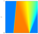
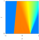
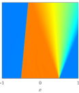
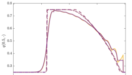
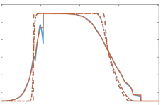
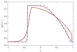
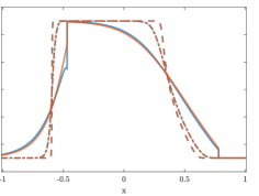
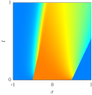
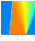
This is why we will tackle the problem in this contribution and prove under specific conditions the convergence to the local entropy solution. We refer the reader in particular to the main Theorem 4.11 of this contribution. The convergence is numerically illustrated in Fig. 1 for the exponential kernel and an archetypal initial datum. As can be observed, the right most illustration is not to be distinguished from the local entropy solution.
Refer to caption
Refer to caption
Refer to caption
Figure 1: Exponential kernel γ()η1exp(η1)\gamma(\cdot)\equiv\eta^{-1}\exp(-\cdot\eta^{-1}), q014+12χ[0.5,0.5]subscript𝑞01412subscript𝜒0.50.5q_{0}\equiv\tfrac{1}{4}+\tfrac{1}{2}\chi_{[-0.5,0.5]}, Nonlocal in the velocity, V()=1()2𝑉1superscript2V(\cdot)=1-(\cdot)^{2}, from left to right η{101,102,103}𝜂superscript101superscript102superscript103\eta\in\{10^{-1},10^{-2},10^{-3}\}, Colorbar: 000\ Refer to caption 11\,1

1.1 Outline

In Section 1 we have motivated the problem setup and have presented it in the relation to already existing literature. Section 2 presents results on well-posedness, stability and a maximum principle for the nonlocal (in the velocity) conservation laws, while Section 3 presents the related local conservation laws and some of their properties particularly the entropy formulation, and more. In Section 4 we choose an exponential kernel for the nonlocal velocity and obtain under additional conditions on the velocity and initial datum a uniform 𝖳𝖵𝖳𝖵\mathsf{TV} bound on the nonlocal velocity is obtained which is used to pass to the limit. However, this limit is only a weak solution but the entropy condition (for the limit, the local case) is open. This is what is established in Theorem 4.8 under slightly more restrictive conditions on the initial datum and the velocity. The chosen approach is reminiscent to [40]. Although this result might be generalizable to a variety of other kernels in the spirit of [17] we do not take this path, but instead look – for general kernels – into the monotonicity of the proposed dynamics. And indeed, in Section 5 we find similar as in [37] without additional restrictions on the velocity that the “nonlocal in the velocity conservation laws” are monotonicity preserving which makes it possible to pass to the limit for monotonically increasing and decreasing datum. We thus cover the archetypes of local conservation laws, rare factions and shock waves. In Section 6, the results are illustrated numerically and the convergence nonlocal in the solution vs. nonlocal in the velocity is compared when the nonlocal kernel approaches a Dirac distribution.

Section 7 concludes the contribution with a list of open problems and future research.

2 Basic results on nonlocal (in velocity) conservation laws

In this section, we present the general assumptions on the involved data, introduce the considered problem class rigorously and define what we mean by weak solutions. Additionally, we provide existence and uniqueness results for the corresponding weak solutions as well as a stability in the initial datum and a maximum principle.

For the rest of the paper, we make the following assumptions which become meaningful when taking a look at Definition 2.1 and Definition 2.2. {assumption}[Nonlocal conservation laws] We assume the following

  • initial datum q0𝖫(;0)𝖳𝖵()subscript𝑞0superscript𝖫subscriptabsent0𝖳𝖵q_{0}\in{\mathsf{L}\!}^{\infty}(\mathbb{R};\mathbb{R}_{\geq 0})\cap\mathsf{TV}(\mathbb{R})

  • velocity function V𝖢2():V0:𝑉superscript𝖢2superscript𝑉0V\in\mathsf{C}^{2}(\mathbb{R}):V^{\prime}\leqq 0

  • nonlocal weight γ𝖫(;0)𝖫1()𝛾superscript𝖫subscriptabsent0superscript𝖫1\gamma\in{\mathsf{L}\!}^{\infty}(\mathbb{R};\mathbb{R}_{\geq 0})\cap{\mathsf{L}\!}^{1}(\mathbb{R}) and γ𝛾\gamma monotonically decreasing,

  • and nonlocal “reach” η>0𝜂subscriptabsent0\eta\in\mathbb{R}_{>0}

and set ΩT(0,T)×subscriptΩ𝑇0𝑇{\Omega_{T}}\mathrel{\coloneqq}(0,T)\times\mathbb{R} for T>0𝑇subscriptabsent0T\in\mathbb{R}_{>0} the considered time horizon. Having stated the assumptions on the input datum of the nonlocal dynamics we now specify these dynamics:

Definition 2.1 (Nonlocal dynamics).

Given Section 2, the nonlocal dynamics, the conservation law with nonlocal velocity, reads as

(2) tq(t,x)subscript𝑡𝑞𝑡𝑥\displaystyle\partial_{t}q(t,x) =x(q(t,x)𝒲[γ,V(q)](t,x)),absentsubscript𝑥𝑞𝑡𝑥𝒲𝛾𝑉𝑞𝑡𝑥\displaystyle=-\partial_{x}\Big{(}q(t,x)\mathcal{W}\big{[}\gamma,V(q)\big{]}(t,x)\Big{)}, (t,x)ΩT,𝑡𝑥subscriptΩ𝑇\displaystyle(t,x)\in{\Omega_{T}},
(3) q(0,x)𝑞0𝑥\displaystyle q(0,x) =q0(x),absentsubscript𝑞0𝑥\displaystyle=q_{0}(x), x,𝑥\displaystyle x\in\mathbb{R},
(4) 𝒲[V(q),γ](t,x)𝒲𝑉𝑞𝛾𝑡𝑥\displaystyle\!\mathcal{W}\big{[}V(q),\!\gamma\big{]}(t,x) (γV(q))(t,x)1ηxγ(yxη)V(q(t,y))dy,absent𝛾𝑉𝑞𝑡𝑥1𝜂superscriptsubscript𝑥𝛾𝑦𝑥𝜂𝑉𝑞𝑡𝑦differential-d𝑦\displaystyle\mathrel{\coloneqq}\big{(}\gamma\ast V(q)\big{)}(t,x)\mathrel{\coloneqq}\tfrac{1}{\eta}\!\int_{x}^{\infty}\!\!\!\!\gamma\big{(}\tfrac{y-x}{\eta}\big{)}V(q(t,y))\,\mathrm{d}y,\!\!\! (t,x)ΩT.𝑡𝑥subscriptΩ𝑇\displaystyle(t,x)\in{\Omega_{T}}.

We call q0::subscript𝑞0q_{0}:\mathbb{R}\rightarrow\mathbb{R} initial datum, V::𝑉V:\mathbb{R}\rightarrow\mathbb{R} the velocity function, γ:00:𝛾subscriptabsent0subscriptabsent0\gamma:\mathbb{R}_{\geq 0}\rightarrow\mathbb{R}_{\geq 0} the nonlocal kernel or weight and 𝒲:ΩT:𝒲subscriptΩ𝑇\mathcal{W}:{\Omega_{T}}\rightarrow\mathbb{R} the nonlocal velocity or nonlocal term for the nonlocal reach η>0𝜂subscriptabsent0\eta\in\mathbb{R}_{>0}.

Given the problem setup we will consider in this work we define what we mean with weak solutions and then address the questions of existence and uniqueness of these.

Definition 2.2 (Weak solution).

Let (T,η)>02𝑇𝜂superscriptsubscriptabsent02(T,\eta)\in\mathbb{R}_{>0}^{2} be given as well as Section 2, we call qη𝖢([0,T];𝖫loc1())𝖫((0,T);𝖫()𝖳𝖵())subscript𝑞𝜂𝖢0𝑇subscriptsuperscript𝖫1locsuperscript𝖫0𝑇superscript𝖫𝖳𝖵q_{\eta}\in\mathsf{C}\big{(}[0,T];{\mathsf{L}\!}^{1}_{\,\textnormal{loc}}(\mathbb{R})\big{)}\cap{\mathsf{L}\!}^{\infty}((0,T);{\mathsf{L}\!}^{\infty}(\mathbb{R})\cap\mathsf{TV}(\mathbb{R})) a weak solution of the nonlocal dynamics in Definition 2.1 iff ϕ𝖢c1((42,T)×)for-allitalic-ϕsubscriptsuperscript𝖢1c42𝑇\forall\phi\in\mathsf{C}^{1}_{\text{c}}((-42,T)\times\mathbb{R}) and for the nonlocal velocity 𝒲[V(q),γ]𝖢([0,T];𝖫loc1())𝒲𝑉𝑞𝛾𝖢0𝑇subscriptsuperscript𝖫1loc\mathcal{W}\big{[}V(q),\gamma\big{]}\in\mathsf{C}\big{(}[0,T];{\mathsf{L}\!}^{1}_{\,\textnormal{loc}}(\mathbb{R})\big{)} as in Eq. 4 it holds that

ΩTq(t,x)(tϕ(t,x)+𝒲[V(q),γ](t,x)xϕ(t,x))dxdt+q0(x)ϕ(0,x)dx=0.subscriptdouble-integralsubscriptΩ𝑇𝑞𝑡𝑥subscript𝑡italic-ϕ𝑡𝑥𝒲𝑉𝑞𝛾𝑡𝑥subscript𝑥italic-ϕ𝑡𝑥differential-d𝑥differential-d𝑡subscriptsubscript𝑞0𝑥italic-ϕ0𝑥differential-d𝑥0\displaystyle\iint_{{\Omega_{T}}}\!\!q(t,x)\Big{(}\partial_{t}\phi(t,x)+\mathcal{W}[V(q),\gamma](t,x)\partial_{x}\phi(t,x)\Big{)}\,\mathrm{d}x\,\mathrm{d}t+\!\int_{\mathbb{R}}q_{0}(x)\phi(0,x)\,\mathrm{d}x=0.

We then have the following existence and uniqueness result on small time horizon.

Theorem 2.3 (Existence & Uniqueness on small time horizon).

Let Section 2 hold. Then, there is a time T>0superscript𝑇subscriptabsent0T^{*}\in\mathbb{R}_{>0} on which there is a unique weak solution

q𝖢([0,T];𝖫loc1())𝖫((0,T);𝖫()𝖳𝖵()).𝑞𝖢0superscript𝑇subscriptsuperscript𝖫1locsuperscript𝖫0superscript𝑇superscript𝖫𝖳𝖵q\in\mathsf{C}\big{(}[0,T^{*}];{\mathsf{L}\!}^{1}_{\,\textnormal{loc}}(\mathbb{R})\big{)}\cap{\mathsf{L}\!}^{\infty}\big{(}(0,T^{*});{\mathsf{L}\!}^{\infty}(\mathbb{R})\cap\mathsf{TV}(\mathbb{R})\big{)}.

Additionally, the solution is nonnegative.

Proof 2.4.

The proof is very similar to [5, Theorem 2.15]. The difference in the considered setup is that the integral operator of the nonlocal term acts not on q𝑞q itself but on V(q)𝑉𝑞V(q) which necessitates to study the related fixed-point problem in the set {𝒲𝖫((0,T);𝖫()):2𝒲𝖫((0,T);𝖳𝖵())}conditional-set𝒲superscript𝖫0𝑇superscript𝖫subscript2𝒲superscript𝖫0𝑇𝖳𝖵\big{\{}\mathcal{W}\in{\mathsf{L}\!}^{\infty}((0,T);{\mathsf{L}\!}^{\infty}(\mathbb{R})):\partial_{2}\mathcal{W}\in{\mathsf{L}\!}^{\infty}((0,T);\mathsf{TV}(\mathbb{R}))\big{\}}. The key idea is to assume that the velocity 𝒲0𝖫((0,T);𝖶1,())superscript𝒲0superscript𝖫0𝑇superscript𝖶1\mathcal{W}^{0}\in{\mathsf{L}\!}^{\infty}((0,T);\mathsf{W}^{1,\infty}(\mathbb{R})) is given and that we can construct the solution of the linear conservation law

tq(t,x)+x(𝒲0(t,x)q(t,x))subscript𝑡𝑞𝑡𝑥subscript𝑥superscript𝒲0𝑡𝑥𝑞𝑡𝑥\displaystyle\partial_{t}q(t,x)+\partial_{x}\big{(}\mathcal{W}^{0}(t,x)q(t,x)\big{)} =0absent0\displaystyle=0
q(0,x)𝑞0𝑥\displaystyle q(0,x) =q0(x)absentsubscript𝑞0𝑥\displaystyle=q_{0}(x)

by means of the characteristics as

(5) q(t,x)=q0(ξ𝒲0(t,x;0))2ξ𝒲0(t,x;0)𝑞𝑡𝑥subscript𝑞0subscript𝜉superscript𝒲0𝑡𝑥0subscript2subscript𝜉superscript𝒲0𝑡𝑥0q(t,x)=q_{0}\big{(}\xi_{\mathcal{W}^{0}}(t,x;0)\big{)}\partial_{2}\xi_{\mathcal{W}^{0}}(t,x;0)

with the characteristics being the unique solution of

(6) ξ(t,x;τ)=x+tτ𝒲0(s,ξ(t,x;s))ds.𝜉𝑡𝑥𝜏𝑥superscriptsubscript𝑡𝜏superscript𝒲0𝑠𝜉𝑡𝑥𝑠differential-d𝑠\xi(t,x;\tau)=x+\int_{t}^{\tau}\mathcal{W}^{0}(s,\xi(t,x;s))\,\mathrm{d}s.

Computing the nonlocal term via Eq. 4 we end up with

(7) 𝒲1(t,x)=1ηxγ(yxη)V(q(t,y))dy=1ηxγ(yxη)V(q0(ξ𝒲0(t,y;0))2ξ𝒲0(t,y;0))dysuperscript𝒲1𝑡𝑥1𝜂superscriptsubscript𝑥𝛾𝑦𝑥𝜂𝑉𝑞𝑡𝑦differential-d𝑦1𝜂superscriptsubscript𝑥𝛾𝑦𝑥𝜂𝑉subscript𝑞0subscript𝜉superscript𝒲0𝑡𝑦0subscript2subscript𝜉superscript𝒲0𝑡𝑦0differential-d𝑦\begin{split}\mathcal{W}^{1}(t,x)&=\tfrac{1}{\eta}\int_{x}^{\infty}\gamma\big{(}\tfrac{y-x}{\eta}\big{)}V(q(t,y))\,\mathrm{d}y\\ &=\tfrac{1}{\eta}\int_{x}^{\infty}\gamma\big{(}\tfrac{y-x}{\eta}\big{)}V\Big{(}q_{0}\big{(}\xi_{\mathcal{W}^{0}}(t,y;0)\big{)}\partial_{2}\xi_{\mathcal{W}^{0}}(t,y;0)\Big{)}\,\mathrm{d}y\end{split}

and inductively for n1𝑛subscriptabsent1n\in\mathbb{N}_{\geq 1}

(8) 𝒲n(t,x)=1ηxγ(yxη)V(q0(ξ𝒲n1(t,y;0))2ξ𝒲n1(t,y;0))dysuperscript𝒲𝑛𝑡𝑥1𝜂superscriptsubscript𝑥𝛾𝑦𝑥𝜂𝑉subscript𝑞0subscript𝜉superscript𝒲𝑛1𝑡𝑦0subscript2subscript𝜉superscript𝒲𝑛1𝑡𝑦0differential-d𝑦\mathcal{W}^{n}(t,x)=\tfrac{1}{\eta}\int_{x}^{\infty}\gamma\big{(}\tfrac{y-x}{\eta}\big{)}V\Big{(}q_{0}\big{(}\xi_{\mathcal{W}^{n-1}}(t,y;0)\big{)}\partial_{2}\xi_{\mathcal{W}^{n-1}}(t,y;0)\Big{)}\,\mathrm{d}y

with ξ𝒲subscript𝜉𝒲\xi_{\mathcal{W}} for 𝒲𝖫((0,T);𝖶loc1,())𝒲superscript𝖫0𝑇subscriptsuperscript𝖶1loc\mathcal{W}\in{\mathsf{L}\!}^{\infty}((0,T);\mathsf{W}^{1,\infty}_{\textnormal{loc}}(\mathbb{R})) as in Eq. 6.

However, this can be interpreted as a fixed-point problem in 𝒲𝒲\mathcal{W} in the topology 𝖫((0,T);𝖫())superscript𝖫0𝑇superscript𝖫{\mathsf{L}\!}^{\infty}((0,T);{\mathsf{L}\!}^{\infty}(\mathbb{R})) and by applying Lipschitz-estimates of the characteristics with regard to the nonlocal term 𝒲𝒲\mathcal{W} (see in particular [38, Theorem 2.4]) and corresponding 𝖳𝖵𝖳𝖵\mathsf{TV} estimates, we can indeed establish by means of Banach’s fixed-point theorem the existence and uniqueness of a solution of Eq. 8. The uniqueness then carries over to the solution as well (compare again [5, Theorem 2.15]) and the nonnegativity of the solution follows from the identity Eq. 5 and the fact that 2ξ>0subscript2𝜉0\partial_{2}\xi>0. We do not detail it further.

As we will later obtain results on the convergence (compare Sections 4 and 5) by means of approximating the nonlocal solution by smooth solutions as well as the maximum principle in Theorem 2.7 we present the following stability result with respect to the initial datum:

Lemma 2.5 (Stability and approximation by strong solutions).

Let the datum as in Section 2 be given and take a standard mollifier {ϕε}ε>0𝖢(;0)subscriptsubscriptitalic-ϕ𝜀𝜀subscriptabsent0superscript𝖢subscriptabsent0\{\phi_{\varepsilon}\}_{\varepsilon\in\mathbb{R}_{>0}}\subset\mathsf{C}^{\infty}(\mathbb{R};\mathbb{R}_{\geq 0}) as in [48, Remark C.18]. Assume that qεsuperscript𝑞𝜀q^{\varepsilon} is for ε>0𝜀subscriptabsent0\varepsilon\in\mathbb{R}_{>0} the solution of the dynamics in Definition 2.1 for the initial datum ϕεq0subscriptitalic-ϕ𝜀subscript𝑞0\phi_{\varepsilon}\ast q_{0} and q𝑞q correspondingly the solution for the initial datum q0subscript𝑞0q_{0}. Then, it holds on a small enough time horizon T>0𝑇subscriptabsent0T\in\mathbb{R}_{>0}

limε0qεq𝖢([0,T];𝖫1())=0subscript𝜀0subscriptnormsuperscript𝑞𝜀𝑞𝖢0𝑇superscript𝖫10\lim_{\varepsilon\rightarrow 0}\|q^{\varepsilon}-q\|_{\mathsf{C}([0,T];{\mathsf{L}\!}^{1}(\mathbb{R}))}=0

and {qε}ε>0𝖢1(ΩT).subscriptsuperscript𝑞𝜀𝜀subscriptabsent0superscript𝖢1subscriptΩ𝑇\{q^{\varepsilon}\}_{\varepsilon\in\mathbb{R}_{>0}}\subset\mathsf{C}^{1}({\Omega_{T}}). In addition, for V𝖢3()𝑉superscript𝖢3V\in\mathsf{C}^{3}(\mathbb{R}) it holds {qε}ε>0𝖢2(ΩT)subscriptsuperscript𝑞𝜀𝜀subscriptabsent0superscript𝖢2subscriptΩ𝑇\{q^{\varepsilon}\}_{\varepsilon\in\mathbb{R}_{>0}}\subset\mathsf{C}^{2}({\Omega_{T}}).

Proof 2.6.

The stability estimate is very reminiscent to the existence and uniqueness Theorem 2.3 proof by means of characteristics. However, the uniform 𝖳𝖵𝖳𝖵\mathsf{TV} bound is crucial to obtain the stability of the solution in 𝖢([0,T];𝖫1())𝖢0𝑇superscript𝖫1\mathsf{C}\big{(}[0,T];{\mathsf{L}\!}^{1}(\mathbb{R})\big{)}. We do not go into details. The small time horizon T>0𝑇subscriptabsent0T\in\mathbb{R}_{>0} on which the stability result holds can be extend to any finite time horizon as long as the corresponding solutions exist on these.

To be able to extend the solveability to any finite time horizon but also to demonstrate the physical reasonability of the model (density is bounded between 00 and a maximal density) we state the following maximum principle:

Theorem 2.7 (Existence & uniqueness of solutions, maximum principle).

Given Section 2, the nonlocal conservation law in Definition 2.1 admits on every finite time horizon T>0𝑇subscriptabsent0T\in\mathbb{R}_{>0} a unique weak solution

q𝖢([0,T];𝖫loc1())𝖫((0,T);𝖫()𝖳𝖵())𝑞𝖢0𝑇subscriptsuperscript𝖫1locsuperscript𝖫0𝑇superscript𝖫𝖳𝖵q\in\mathsf{C}\big{(}[0,T];{\mathsf{L}\!}^{1}_{\textnormal{loc}}(\mathbb{R})\big{)}\cap{\mathsf{L}\!}^{\infty}\big{(}(0,T);{\mathsf{L}\!}^{\infty}(\mathbb{R})\cap\mathsf{TV}(\mathbb{R})\big{)}

in the sense of Definition 2.2 and the following maximum principle holds

essinfxq0(x)q(t,x)subscriptessinfimum𝑥subscript𝑞0𝑥𝑞𝑡𝑥\displaystyle\operatorname*{ess-\inf}_{x\in\mathbb{R}}q_{0}(x)\leq q(t,x) esssupxq0(x), for a.e. x,t[0,T].formulae-sequenceabsentsubscriptesssupremum𝑥subscript𝑞0𝑥formulae-sequence for a.e. 𝑥𝑡0𝑇\displaystyle\leq\operatorname*{ess-\sup}_{x\in\mathbb{R}}q_{0}(x),\text{ for a.e. }x\in\mathbb{R},\ t\in[0,T].

Proof 2.8.

We only show the maximum principle and only the upper bound. Approximating the initial datum as in Lemma 2.5 we obtain the corresponding solution qε𝖢1(ΩT)superscript𝑞𝜀superscript𝖢1subscriptΩ𝑇q^{\varepsilon}\in\mathsf{C}^{1}({\Omega_{T}}) so that it indeed satisfies the nonlocal conservation law in the classical sense. Then, we have for (t,x)ΩT𝑡𝑥subscriptΩ𝑇(t,x)\in{\Omega_{T}}

(9) tqε(t,x)subscript𝑡superscript𝑞𝜀𝑡𝑥\displaystyle\partial_{t}q^{\varepsilon}(t,x) =𝒲[V(qε),γ](t,x)xqε(t,x)x𝒲[V(qε),γ](t,x)qε(t,x)absent𝒲𝑉superscript𝑞𝜀𝛾𝑡𝑥subscript𝑥superscript𝑞𝜀𝑡𝑥subscript𝑥𝒲𝑉superscript𝑞𝜀𝛾𝑡𝑥superscript𝑞𝜀𝑡𝑥\displaystyle=-\mathcal{W}[V(q^{\varepsilon}),\gamma](t,x)\partial_{x}q^{\varepsilon}(t,x)-\partial_{x}\mathcal{W}[V(q^{\varepsilon}),\gamma](t,x)q^{\varepsilon}(t,x)
assuming that for given t[0,T]𝑡0𝑇t\in[0,T] we are at a maximal point x𝑥x\in\mathbb{R}, i.e. xqε(t,x)=0subscript𝑥superscript𝑞𝜀𝑡𝑥0\partial_{x}q^{\varepsilon}(t,x)=0
(10) =x𝒲[V(qε),γ](t,x)qε(t,x)absentsubscript𝑥𝒲𝑉superscript𝑞𝜀𝛾𝑡𝑥superscript𝑞𝜀𝑡𝑥\displaystyle=-\partial_{x}\mathcal{W}[V(q^{\varepsilon}),\gamma](t,x)q^{\varepsilon}(t,x)

As qε0superscript𝑞𝜀0q^{\varepsilon}\geqq 0 thanks to Theorem 2.3, we only need to show that x𝒲subscript𝑥𝒲\partial_{x}\mathcal{W} is positive at the maximal value x𝑥x. To this end, write

x𝒲[V(qε),γ](t,x)subscript𝑥𝒲𝑉superscript𝑞𝜀𝛾𝑡𝑥\displaystyle\partial_{x}\mathcal{W}[V(q^{\varepsilon}),\gamma](t,x) =1ηγ(0)V(qε(t,x))1η2xγ(yxη)V(qε(t,y))dyabsent1𝜂𝛾0𝑉superscript𝑞𝜀𝑡𝑥1superscript𝜂2superscriptsubscript𝑥superscript𝛾𝑦𝑥𝜂𝑉superscript𝑞𝜀𝑡𝑦differential-d𝑦\displaystyle=-\tfrac{1}{\eta}\gamma(0)V(q^{\varepsilon}(t,x))-\tfrac{1}{\eta^{2}}\int_{x}^{\infty}\!\!\!\!\gamma^{\prime}\big{(}\tfrac{y-x}{\eta}\big{)}V(q^{\varepsilon}(t,y))\,\mathrm{d}y
and as γ0superscript𝛾0\gamma^{\prime}\leqq 0 and qε(t,x)superscript𝑞𝜀𝑡𝑥q^{\varepsilon}(t,x) maximal so that V(qε(t,x))𝑉superscript𝑞𝜀𝑡𝑥V(q^{\varepsilon}(t,x)) minimal
1ηγ(0)V(qε(t,x))1η2V(qε(t,x))xγ(yxη)dyabsent1𝜂𝛾0𝑉superscript𝑞𝜀𝑡𝑥1superscript𝜂2𝑉superscript𝑞𝜀𝑡𝑥superscriptsubscript𝑥superscript𝛾𝑦𝑥𝜂differential-d𝑦\displaystyle\geq-\tfrac{1}{\eta}\gamma(0)V(q^{\varepsilon}(t,x))-\tfrac{1}{\eta^{2}}V(q^{\varepsilon}(t,x))\int_{x}^{\infty}\gamma^{\prime}\big{(}\tfrac{y-x}{\eta}\big{)}\,\mathrm{d}y
1ηV(qε(t,x))limyγ(yxη)=0absent1𝜂𝑉superscript𝑞𝜀𝑡𝑥subscript𝑦𝛾𝑦𝑥𝜂0\displaystyle\geq\tfrac{1}{\eta}V(q^{\varepsilon}(t,x))\lim\nolimits_{y\rightarrow\infty}\gamma\big{(}\tfrac{y-x}{\eta}\big{)}=0

as γ𝖳𝖵(>0)𝖫1(>0)limyγ(yxη)=0x𝛾𝖳𝖵subscriptabsent0superscript𝖫1subscriptabsent0subscript𝑦𝛾𝑦𝑥𝜂0for-all𝑥\gamma\in\mathsf{TV}(\mathbb{R}_{>0})\cap{\mathsf{L}\!}^{1}(\mathbb{R}_{>0})\implies\lim_{y\rightarrow\infty}\gamma\big{(}\frac{y-x}{\eta}\big{)}=0\ \forall x\in\mathbb{R}.

However, this means that in the maximal point x𝑥x\in\mathbb{R} the time derivative in Eq. 9 is nonpositive, meaning that the maximum cannot increase further. From this, the upper bound on the smoothed solution follows and as these bounds are uniform, they also hold in the limit for the non-smoothed version.

The lower bound can be derived analogously, concluding the proof.

Remark 2.9 (Other ways to obtain the previous results).

The existence of weak solutions and the maximum principle can be proven by following the lines of [28]. As in the latter work the problem in Definition 2.1 is considered with a compactly supported kernel, we need to restrict the support of the kernel onto a compact interval (in an appropriate manner) such that the convergence of the numerical scheme in [28] is ensured. In particular, the estimates obtained in [28] remain valid. We do not go into details here.

3 Fundamental results on (local) conservation laws

As we will study the convergence of solutions qηsubscript𝑞𝜂q_{\eta} for the Cauchy problem in Definition 2.1 we need to cover the well-established theory of local conservation laws which is for instance fundamentally described in [8, 32, 26].

Definition 3.1 (The local conservation law).

Given Definition 2.1 we call the Cauchy problem, the conservation law with initial datum q0subscript𝑞0q_{0},

tq(t,x)+x(V(q(t,x))q(t,x))subscript𝑡𝑞𝑡𝑥subscript𝑥𝑉𝑞𝑡𝑥𝑞𝑡𝑥\displaystyle\partial_{t}q(t,x)+\partial_{x}\big{(}V(q(t,x))q(t,x)\big{)} =0,absent0\displaystyle=0, (t,x)ΩT,𝑡𝑥subscriptΩ𝑇\displaystyle(t,x)\in{\Omega_{T}},
q(0,x)𝑞0𝑥\displaystyle q(0,x) =q0(x),absentsubscript𝑞0𝑥\displaystyle=q_{0}(x), x,𝑥\displaystyle x\in\mathbb{R},

the local conservation law related to the nonlocal (in the velocity) conservation law in Definition 2.1.

For the definition of weak solutions for local conservation laws we refer to Definition 2.2 when replacing the nonlocal term by V(q)𝑉𝑞V(q). However, as it is well-known weak solutions are not necessarily unique in particular as solutions develop discontinuities in finite time. This is why one prescribes additional assumptions on the weak solution, a so called entropy condition. In this work, we will use entropy-flux pairs as it will be detrimental in our later analysis that we can take advantage of a specific entropy to pass to the limit. However, in Remark 5.9 we will later also discuss Oleinik’s entropy condition [2, 51].

Definition 3.2 (Entropy solution – entropy flux pair).

Let Section 2 hold. Then, we call q𝖢([0,T];𝖫loc1())𝖫((0,T);𝖫()𝖳𝖵())𝑞𝖢0𝑇subscriptsuperscript𝖫1locsuperscript𝖫0𝑇superscript𝖫𝖳𝖵q\in\mathsf{C}\big{(}[0,T];{\mathsf{L}\!}^{1}_{\textnormal{loc}}(\mathbb{R})\big{)}\cap{\mathsf{L}\!}^{\infty}((0,T);{\mathsf{L}\!}^{\infty}(\mathbb{R})\cap\mathsf{TV}(\mathbb{R})) an entropy solution to Definition 3.1 iff it satisfies α𝖢2()for-all𝛼superscript𝖢2\forall\alpha\in\mathsf{C}^{2}(\mathbb{R}) convex with β𝖢1()𝛽superscript𝖢1\beta\in\mathsf{C}^{1}(\mathbb{R}) so that

β(x)=α(x)(V(x)+xV(x))xformulae-sequencesuperscript𝛽𝑥superscript𝛼𝑥𝑉𝑥𝑥superscript𝑉𝑥for-all𝑥\beta^{\prime}(x)=\alpha^{\prime}(x)\big{(}V(x)+xV^{\prime}(x)\big{)}\quad\forall x\in\mathbb{R}

ϕ𝖢c1((42;T)×;0)for-allitalic-ϕsubscriptsuperscript𝖢1c42𝑇subscriptabsent0\forall\phi\in\mathsf{C}^{1}_{\text{c}}\big{(}(-42;T)\times\mathbb{R};\mathbb{R}_{\geq 0}\big{)}

(11) [ϕ,α,q]ΩTα(q(t,x))tϕ(t,x)+β(q(t,x))xϕ(t,x)dxdt+α(q0(x))ϕ(0,x)dx0.italic-ϕ𝛼𝑞subscriptdouble-integralsubscriptΩ𝑇𝛼𝑞𝑡𝑥subscript𝑡italic-ϕ𝑡𝑥𝛽𝑞𝑡𝑥subscript𝑥italic-ϕ𝑡𝑥d𝑥d𝑡subscript𝛼subscript𝑞0𝑥italic-ϕ0𝑥differential-d𝑥0\begin{split}\mathcal{EF}[\phi,\alpha,q]&\mathrel{\coloneqq}\iint_{{\Omega_{T}}}\alpha(q(t,x))\partial_{t}\phi(t,x)+\beta(q(t,x))\partial_{x}\phi(t,x)\,\mathrm{d}x\,\mathrm{d}t\\ &\qquad+\int_{\mathbb{R}}\alpha(q_{0}(x))\phi(0,x)\,\mathrm{d}x\geq 0.\end{split}

Having this definition, we obtain the famous existence and uniqueness result for local scalar conservation laws:

Theorem 3.3 (Existence & Uniqueness of entropy solutions).

The local conservation law stated in Definition 3.1 admits a unique entropy solution in the sense of Definition 3.2.

Proof 3.4.

The result can be found in [8, Theorem 6.3] using wave front tracking and a semi-group argument and in [26, Theorem 19.1]. We also refer to [46, Theorem 2, Theorem 5, Section 5 Item 4]. For the introduced flux pair one can find the proof in [32].

As we will later take advantage of the fact that under specific conditions the entropy inequality in Eq. 11 needs to be satisfied for only one entropy flux pair, we provide the following Theorem 3.5 which can be found in [25].

Theorem 3.5 (One strictly concave entropy is enough for uniqueness).

Assume that the flux function f(x)xV(x)x𝑓𝑥𝑥𝑉𝑥for-all𝑥f(x)\mathrel{\coloneqq}xV(x)\ \forall x\in\mathbb{R} is strictly concave, i.e.,

xf′′(x)=xV′′(x)+2V(x)<0xsupp(q0)maps-to𝑥superscript𝑓′′𝑥𝑥superscript𝑉′′𝑥2superscript𝑉𝑥0for-all𝑥suppsubscript𝑞0x\mapsto f^{\prime\prime}(x)=xV^{\prime\prime}(x)+2V^{\prime}(x)<0\ \forall x\in\operatorname{supp}(q_{0})

with V𝑉V as in Section 2 and the function

q𝖢([0,T];𝖫loc1())𝖫((0,T);𝖫()𝖳𝖵())superscript𝑞𝖢0𝑇subscriptsuperscript𝖫1locsuperscript𝖫0𝑇superscript𝖫𝖳𝖵q^{*}\in\mathsf{C}\big{(}[0,T];{\mathsf{L}\!}^{1}_{\textnormal{loc}}(\mathbb{R})\big{)}\cap{\mathsf{L}\!}^{\infty}\big{(}(0,T);{\mathsf{L}\!}^{\infty}(\mathbb{R})\cap\mathsf{TV}(\mathbb{R})\big{)}

satisfies the entropy condition

[ϕ,α,q]0ϕ𝖢c1((42,T)×;0)formulae-sequenceitalic-ϕ𝛼superscript𝑞0for-allitalic-ϕsubscriptsuperscript𝖢1c42𝑇subscriptabsent0\mathcal{EF}[\phi,\alpha,q^{*}]\geq 0\qquad\forall\phi\in\mathsf{C}^{1}_{\text{c}}\big{(}(-42,T)\times\mathbb{R};\mathbb{R}_{\geq 0}\big{)}

as in Eq. 11 for one entropy α𝛼\alpha which is strictly convex. Then, qsuperscript𝑞q^{*} is the unique entropy solution.

Proof 3.6.

The result has been proven in [25, Theorem 2.3 & Corollary 2.5] for strictly convex fluxes f𝑓f and with a small adjustment it also holds for strictly concave flux functions.

4 Convergence – Exponential kernel and arbitrary initial datum

In this section, we will state conditions on velocity V𝑉V and initial datum q0subscript𝑞0q_{0} under which the solution of the nonlocal (in the velocity) conservation law converges to the entropy solution of the local conservation law. We assume that the kernel is of exponential type which is inspired by the approach and ideas in [16].

We start in the following Section 4.1 with proving uniform 𝖳𝖵𝖳𝖵\mathsf{TV} bounds on the nonlocal velocity:

4.1 Uniform total variation bounds on the nonlocal velocity

In this section, we derive a total variation bound on the nonlocal velocity uniformly in η>0𝜂subscriptabsent0\eta\in\mathbb{R}_{>0}. To this end, we first deduce dynamics directly on the nonlocal velocity for nonlocal kernels of exponential type:

Lemma 4.1 (Dynamics in the nonlocal velocity).

Given the unique weak solution of the nonlocal conservation law in Definition 2.1 and recall the definition of the nonlocal velocity Eq. 4, we have for the nonlocal term with exponential weight for η>0𝜂subscriptabsent0\eta\in\mathbb{R}_{>0} and (t,x)ΩT𝑡𝑥subscriptΩ𝑇(t,x)\in{\Omega_{T}} (with an abuse of notation)

(12) 𝒲η[V(qη)](t,x)𝒲η[V(qη),e()](t,x)=1ηxexyηV(qη(t,y))dy,subscript𝒲𝜂delimited-[]𝑉subscript𝑞𝜂𝑡𝑥subscript𝒲𝜂𝑉subscript𝑞𝜂superscripte𝑡𝑥1𝜂superscriptsubscript𝑥superscripte𝑥𝑦𝜂𝑉subscript𝑞𝜂𝑡𝑦differential-d𝑦\mathcal{W}_{\eta}[V(q_{\eta})](t,x)\coloneqq\mathcal{W}_{\eta}\big{[}V(q_{\eta}),\mathrm{e}^{-(\cdot)}\big{]}(t,x)=\tfrac{1}{\eta}\int_{x}^{\infty}\!\!\!\!\mathrm{e}^{\frac{x-y}{\eta}}V(q_{\eta}(t,y))\,\mathrm{d}y,

that 𝒲η[V(qη)]𝖶1,(ΩT)subscript𝒲𝜂delimited-[]𝑉subscript𝑞𝜂superscript𝖶1subscriptΩ𝑇\mathcal{W}_{\eta}[V(q_{\eta})]\in\mathsf{W}^{1,\infty}({\Omega_{T}}) and in addition that 𝒲η[V(q)]subscript𝒲𝜂delimited-[]𝑉𝑞\mathcal{W}_{\eta}[V(q)] satisfies the following dynamics for (t,x)ΩT𝑡𝑥subscriptΩ𝑇(t,x)\in{\Omega_{T}} a.e.

(13) t𝒲η[V(qη)](t,x)=1ηxexzηV(qη(t,z))z𝒲η[V(qη)](t,z)qη(t,z)dz+1η(𝒲η[V(qη)](t,x))21η2xexzηV(qη(t,z))2dzx𝒲η[V(qη)](t,x)𝒲η[V(qη)](t,x).subscript𝑡subscript𝒲𝜂delimited-[]𝑉subscript𝑞𝜂𝑡𝑥1𝜂superscriptsubscript𝑥superscripte𝑥𝑧𝜂superscript𝑉subscript𝑞𝜂𝑡𝑧subscript𝑧subscript𝒲𝜂delimited-[]𝑉subscript𝑞𝜂𝑡𝑧subscript𝑞𝜂𝑡𝑧d𝑧1𝜂superscriptsubscript𝒲𝜂delimited-[]𝑉subscript𝑞𝜂𝑡𝑥21superscript𝜂2superscriptsubscript𝑥superscripte𝑥𝑧𝜂𝑉superscriptsubscript𝑞𝜂𝑡𝑧2differential-d𝑧subscript𝑥subscript𝒲𝜂delimited-[]𝑉subscript𝑞𝜂𝑡𝑥subscript𝒲𝜂delimited-[]𝑉subscript𝑞𝜂𝑡𝑥\begin{split}&\partial_{t}\mathcal{W}_{\eta}[V(q_{\eta})](t,x)\\ &=-\tfrac{1}{\eta}\int_{x}^{\infty}\mathrm{e}^{\frac{x-z}{\eta}}V^{\prime}(q_{\eta}(t,z))\partial_{z}\mathcal{W}_{\eta}[V(q_{\eta})](t,z)q_{\eta}(t,z)\,\mathrm{d}z+\tfrac{1}{\eta}\big{(}\mathcal{W}_{\eta}[V(q_{\eta})](t,x)\big{)}^{2}\\ &\quad-\tfrac{1}{\eta^{2}}\int_{x}^{\infty}\mathrm{e}^{\frac{x-z}{\eta}}V(q_{\eta}(t,z))^{2}\,\mathrm{d}z-\partial_{x}\mathcal{W}_{\eta}[V(q_{\eta})](t,x)\mathcal{W}_{\eta}[V(q_{\eta})](t,x).\end{split}

Proof 4.2.

The proof is a direct consequence of the identity in Eq. 12 which states for the spatial derivative that

(14) ηx𝒲η[V(qη)](t,x)=𝒲η[V(qη)](t,x)V(qη(t,x)),(t,x)ΩT.formulae-sequence𝜂subscript𝑥subscript𝒲𝜂delimited-[]𝑉subscript𝑞𝜂𝑡𝑥subscript𝒲𝜂delimited-[]𝑉subscript𝑞𝜂𝑡𝑥𝑉subscript𝑞𝜂𝑡𝑥for-all𝑡𝑥subscriptΩ𝑇\eta\partial_{x}\mathcal{W}_{\eta}[V(q_{\eta})](t,x)=\mathcal{W}_{\eta}[V(q_{\eta})](t,x)-V(q_{\eta}(t,x)),\quad\forall(t,x)\in{\Omega_{T}}.

As some of the necessary transformations require higher regularity, the stability result in Lemma 2.5 to smooth the solution qηsubscript𝑞𝜂q_{\eta} by qηε,ε>0,superscriptsubscript𝑞𝜂𝜀𝜀subscriptabsent0q_{\eta}^{\varepsilon},\ \varepsilon\in\mathbb{R}_{>0}, plays a crucial role: So let us assume that we have such a smooth solution qηε𝖢1(ΩT)superscriptsubscript𝑞𝜂𝜀superscript𝖢1subscriptΩ𝑇q_{\eta}^{\varepsilon}\in\mathsf{C}^{1}({\Omega_{T}}). Then, we can start with the time derivative of the nonlocal velocity and have in a weak sense for (t,x)ΩT𝑡𝑥subscriptΩ𝑇(t,x)\in{\Omega_{T}}

t𝒲η[V(qηε)](t,x)subscript𝑡subscript𝒲𝜂delimited-[]𝑉superscriptsubscript𝑞𝜂𝜀𝑡𝑥\displaystyle\partial_{t}\mathcal{W}_{\eta}[V(q_{\eta}^{\varepsilon})](t,x) =1ηxexyηV(qηε(t,y))tqηε(t,y)dyabsent1𝜂superscriptsubscript𝑥superscripte𝑥𝑦𝜂superscript𝑉superscriptsubscript𝑞𝜂𝜀𝑡𝑦subscript𝑡superscriptsubscript𝑞𝜂𝜀𝑡𝑦d𝑦\displaystyle=\tfrac{1}{\eta}\int_{x}^{\infty}\mathrm{e}^{\frac{x-y}{\eta}}V^{\prime}(q_{\eta}^{\varepsilon}(t,y))\partial_{t}q_{\eta}^{\varepsilon}(t,y)\,\mathrm{d}y
and as qηεsuperscriptsubscript𝑞𝜂𝜀q_{\eta}^{\varepsilon} is a classical solution of Definition 2.1
=1ηxexyηV(qηε(t,y))y(qηε(t,y)𝒲η[V(qηε)](t,y))dyabsent1𝜂superscriptsubscript𝑥superscripte𝑥𝑦𝜂superscript𝑉superscriptsubscript𝑞𝜂𝜀𝑡𝑦subscript𝑦superscriptsubscript𝑞𝜂𝜀𝑡𝑦subscript𝒲𝜂delimited-[]𝑉superscriptsubscript𝑞𝜂𝜀𝑡𝑦d𝑦\displaystyle=-\tfrac{1}{\eta}\int_{x}^{\infty}\mathrm{e}^{\frac{x-y}{\eta}}V^{\prime}(q_{\eta}^{\varepsilon}(t,y))\partial_{y}\big{(}q_{\eta}^{\varepsilon}(t,y)\mathcal{W}_{\eta}[V(q_{\eta}^{\varepsilon})](t,y)\big{)}\,\mathrm{d}y
=1ηxexyηV(qηε(t,y))qηε(t,y)y𝒲η[V(qηε)](t,y)dyabsent1𝜂superscriptsubscript𝑥superscripte𝑥𝑦𝜂superscript𝑉superscriptsubscript𝑞𝜂𝜀𝑡𝑦superscriptsubscript𝑞𝜂𝜀𝑡𝑦subscript𝑦subscript𝒲𝜂delimited-[]𝑉superscriptsubscript𝑞𝜂𝜀𝑡𝑦d𝑦\displaystyle=-\tfrac{1}{\eta}\int_{x}^{\infty}\mathrm{e}^{\frac{x-y}{\eta}}V^{\prime}(q_{\eta}^{\varepsilon}(t,y))q_{\eta}^{\varepsilon}(t,y)\partial_{y}\mathcal{W}_{\eta}[V(q_{\eta}^{\varepsilon})](t,y)\,\mathrm{d}y
1ηxexyηV(qηε(t,y))yqηε(t,y)𝒲η[V(qηε)](t,y)dy1𝜂superscriptsubscript𝑥superscripte𝑥𝑦𝜂superscript𝑉superscriptsubscript𝑞𝜂𝜀𝑡𝑦subscript𝑦superscriptsubscript𝑞𝜂𝜀𝑡𝑦subscript𝒲𝜂delimited-[]𝑉superscriptsubscript𝑞𝜂𝜀𝑡𝑦d𝑦\displaystyle\qquad-\tfrac{1}{\eta}\int_{x}^{\infty}\mathrm{e}^{\frac{x-y}{\eta}}V^{\prime}(q_{\eta}^{\varepsilon}(t,y))\partial_{y}q_{\eta}^{\varepsilon}(t,y)\mathcal{W}_{\eta}[V(q_{\eta}^{\varepsilon})](t,y)\,\mathrm{d}y
and integration by parts in the latter term
=1ηxexyηV(qηε(t,y))qηε(t,y)y𝒲η[V(qηε)](t,y)dyabsent1𝜂superscriptsubscript𝑥superscripte𝑥𝑦𝜂superscript𝑉superscriptsubscript𝑞𝜂𝜀𝑡𝑦superscriptsubscript𝑞𝜂𝜀𝑡𝑦subscript𝑦subscript𝒲𝜂delimited-[]𝑉superscriptsubscript𝑞𝜂𝜀𝑡𝑦d𝑦\displaystyle=-\tfrac{1}{\eta}\int_{x}^{\infty}\mathrm{e}^{\frac{x-y}{\eta}}V^{\prime}(q_{\eta}^{\varepsilon}(t,y))q_{\eta}^{\varepsilon}(t,y)\partial_{y}\mathcal{W}_{\eta}[V(q_{\eta}^{\varepsilon})](t,y)\,\mathrm{d}y
+1ηxexyηV(qηε(t,y))y𝒲η[V(qηε)](t,y)dy1𝜂superscriptsubscript𝑥superscripte𝑥𝑦𝜂𝑉superscriptsubscript𝑞𝜂𝜀𝑡𝑦subscript𝑦subscript𝒲𝜂delimited-[]𝑉superscriptsubscript𝑞𝜂𝜀𝑡𝑦d𝑦\displaystyle\qquad+\tfrac{1}{\eta}\int_{x}^{\infty}\mathrm{e}^{\frac{x-y}{\eta}}V(q_{\eta}^{\varepsilon}(t,y))\partial_{y}\mathcal{W}_{\eta}[V(q_{\eta}^{\varepsilon})](t,y)\,\mathrm{d}y
1η2xexyηV(qηε(t,y))𝒲η[V(qηε)](t,y)dy1superscript𝜂2superscriptsubscript𝑥superscripte𝑥𝑦𝜂𝑉superscriptsubscript𝑞𝜂𝜀𝑡𝑦subscript𝒲𝜂delimited-[]𝑉superscriptsubscript𝑞𝜂𝜀𝑡𝑦differential-d𝑦\displaystyle\qquad-\tfrac{1}{\eta^{2}}\int_{x}^{\infty}\mathrm{e}^{\frac{x-y}{\eta}}V(q_{\eta}^{\varepsilon}(t,y))\mathcal{W}_{\eta}[V(q_{\eta}^{\varepsilon})](t,y)\,\mathrm{d}y
+1ηV(qηε(t,x))𝒲η[V(qηε)](t,x)1𝜂𝑉superscriptsubscript𝑞𝜂𝜀𝑡𝑥subscript𝒲𝜂delimited-[]𝑉superscriptsubscript𝑞𝜂𝜀𝑡𝑥\displaystyle\qquad+\tfrac{1}{\eta}V(q_{\eta}^{\varepsilon}(t,x))\mathcal{W}_{\eta}[V(q_{\eta}^{\varepsilon})](t,x)
=(14)1ηxexyηV(qηε(t,y))qηε(t,y)y𝒲η[V(qηε)](t,y)dyitalic-(14italic-)1𝜂superscriptsubscript𝑥superscripte𝑥𝑦𝜂superscript𝑉superscriptsubscript𝑞𝜂𝜀𝑡𝑦superscriptsubscript𝑞𝜂𝜀𝑡𝑦subscript𝑦subscript𝒲𝜂delimited-[]𝑉superscriptsubscript𝑞𝜂𝜀𝑡𝑦d𝑦\displaystyle\overset{\eqref{eq:nonlocal_derivative}}{=}-\tfrac{1}{\eta}\int_{x}^{\infty}\mathrm{e}^{\frac{x-y}{\eta}}V^{\prime}(q_{\eta}^{\varepsilon}(t,y))q_{\eta}^{\varepsilon}(t,y)\partial_{y}\mathcal{W}_{\eta}[V(q_{\eta}^{\varepsilon})](t,y)\,\mathrm{d}y
1η2xexyηV(qηε(t,y))2dy1superscript𝜂2superscriptsubscript𝑥superscripte𝑥𝑦𝜂𝑉superscriptsuperscriptsubscript𝑞𝜂𝜀𝑡𝑦2differential-d𝑦\displaystyle\qquad-\tfrac{1}{\eta^{2}}\int_{x}^{\infty}\mathrm{e}^{\frac{x-y}{\eta}}V(q_{\eta}^{\varepsilon}(t,y))^{2}\,\mathrm{d}y
+1η(𝒲η[V(qηε)](t,x))2𝒲η[V(qηε)](t,x)x𝒲η[V(qηε)](t,x).1𝜂superscriptsubscript𝒲𝜂delimited-[]𝑉superscriptsubscript𝑞𝜂𝜀𝑡𝑥2subscript𝒲𝜂delimited-[]𝑉superscriptsubscript𝑞𝜂𝜀𝑡𝑥subscript𝑥subscript𝒲𝜂delimited-[]𝑉superscriptsubscript𝑞𝜂𝜀𝑡𝑥\displaystyle\qquad+\tfrac{1}{\eta}\big{(}\mathcal{W}_{\eta}[V(q_{\eta}^{\varepsilon})](t,x)\big{)}^{2}-\mathcal{W}_{\eta}[V(q_{\eta}^{\varepsilon})](t,x)\partial_{x}\mathcal{W}_{\eta}[V(q_{\eta}^{\varepsilon})](t,x).

However, letting ε0𝜀0\varepsilon\rightarrow 0 we obtain the claimed Eq. 13.

Having derived the equation in 𝒲η[V(qη)]subscript𝒲𝜂delimited-[]𝑉subscript𝑞𝜂\mathcal{W}_{\eta}[V(q_{\eta})] in Lemma 4.1 we can use this to obtain a uniform total variation estimate in the nonlocal version of the velocity. However, before doing so we prove another estimate which is required afterwards and establishes some behavior of the spatial derivative of the nonlocal term around negative infinity.

Lemma 4.3 (Vanishing 2𝒲ηsubscript2subscript𝒲𝜂\partial_{2}\mathcal{W}_{\eta} at negative infinity).

Let Section 2 hold. Then, we have for q𝖳𝖵()𝖢1()𝑞𝖳𝖵superscript𝖢1q\in\mathsf{TV}(\mathbb{R})\cap\mathsf{C}^{1}(\mathbb{R}) with 𝒲ηsubscript𝒲𝜂\mathcal{W}_{\eta} the nonlocal operator as in Eq. 12

limxx𝒲η[V(q)](x)=0.subscript𝑥subscript𝑥subscript𝒲𝜂delimited-[]𝑉𝑞𝑥0\lim_{x\rightarrow-\infty}\partial_{x}\mathcal{W}_{\eta}[V(q)](x)=0.

Proof 4.4.

We have for all x𝑥x\in\mathbb{R} and yxsuperscript𝑦subscriptabsent𝑥y^{*}\in\mathbb{R}_{\geq x}

|x𝒲η[V(q)](x)|subscript𝑥subscript𝒲𝜂delimited-[]𝑉𝑞𝑥\displaystyle\big{|}\partial_{x}\mathcal{W}_{\eta}[V(q)](x)\big{|} =|𝒲η[V(q)q](x)|absentsubscript𝒲𝜂delimited-[]superscript𝑉𝑞superscript𝑞𝑥\displaystyle=\big{|}\mathcal{W}_{\eta}\big{[}V^{\prime}(q)q^{\prime}\big{]}(x)\big{|}
1ηxyexyη|V(q(y))||q(y)|dy+1ηyexyη|V(q(y))||q(y)|dyabsent1𝜂superscriptsubscript𝑥superscript𝑦superscripte𝑥𝑦𝜂superscript𝑉𝑞𝑦superscript𝑞𝑦differential-d𝑦1𝜂superscriptsubscriptsuperscript𝑦superscripte𝑥𝑦𝜂superscript𝑉𝑞𝑦superscript𝑞𝑦differential-d𝑦\displaystyle\leq\tfrac{1}{\eta}\int_{x}^{y^{*}}\mathrm{e}^{\frac{x-y}{\eta}}|V^{\prime}(q(y))||q^{\prime}(y)|\,\mathrm{d}y+\tfrac{1}{\eta}\int_{y^{*}}^{\infty}\mathrm{e}^{\frac{x-y}{\eta}}|V^{\prime}(q(y))||q^{\prime}(y)|\,\mathrm{d}y
1ηy|V(q(y))||q(y)|dy+1ηyexyη|V(q(y))||q(y)|dyabsent1𝜂superscriptsubscriptsuperscript𝑦superscript𝑉𝑞𝑦superscript𝑞𝑦differential-d𝑦1𝜂superscriptsubscriptsuperscript𝑦superscripte𝑥𝑦𝜂superscript𝑉𝑞𝑦superscript𝑞𝑦differential-d𝑦\displaystyle\leq\tfrac{1}{\eta}\int_{-\infty}^{y^{*}}|V^{\prime}(q(y))||q^{\prime}(y)|\,\mathrm{d}y+\tfrac{1}{\eta}\int_{y^{*}}^{\infty}\mathrm{e}^{\frac{x-y}{\eta}}|V^{\prime}(q(y))||q^{\prime}(y)|\,\mathrm{d}y
1ηV𝖫((0,q𝖫()))|q|𝖳𝖵(,y)+1ηyexyη|V(q(y))||q(y)|dy.absent1𝜂subscriptnormsuperscript𝑉superscript𝖫0subscriptnorm𝑞superscript𝖫subscript𝑞𝖳𝖵superscript𝑦1𝜂superscriptsubscriptsuperscript𝑦superscripte𝑥𝑦𝜂superscript𝑉𝑞𝑦superscript𝑞𝑦differential-d𝑦\displaystyle\leq\tfrac{1}{\eta}\|V^{\prime}\|_{{\mathsf{L}\!}^{\infty}((0,\|q\|_{{\mathsf{L}\!}^{\infty}(\mathbb{R})}))}|q|_{\mathsf{TV}(-\infty,y^{*})}+\tfrac{1}{\eta}\int_{y^{*}}^{\infty}\mathrm{e}^{\frac{x-y}{\eta}}|V^{\prime}(q(y))||q^{\prime}(y)|\,\mathrm{d}y.

We can chose y<0superscript𝑦subscriptabsent0y^{*}\in\mathbb{R}_{<0} negative enough so that |q|𝖳𝖵(,y)subscript𝑞𝖳𝖵superscript𝑦|q|_{\mathsf{TV}(-\infty,y^{*})} is arbitrary small and letting x𝑥x\rightarrow-\infty in the second term, we have by the monotone convergence that this term vanishes. Altogether, we obtain

limx|x𝒲η[V(qη)](x)|=0.subscript𝑥subscript𝑥subscript𝒲𝜂delimited-[]𝑉subscript𝑞𝜂𝑥0\lim_{x\rightarrow-\infty}|\partial_{x}\mathcal{W}_{\eta}[V(q_{\eta})](x)|=0.

The next proposition establishes uniform 𝖳𝖵𝖳𝖵\mathsf{TV} bounds on the nonlocal velocity as long as the velocity function V𝑉V satisfies a specific growth condition:

Proposition 4.5 (Uniform (in η𝜂\eta) total variation estimate of 𝒲η[V(qη)]subscript𝒲𝜂delimited-[]𝑉subscript𝑞𝜂\mathcal{W}_{\eta}[V(q_{\eta})]).

Let 𝒲η[V(qη)]subscript𝒲𝜂delimited-[]𝑉subscript𝑞𝜂\mathcal{W}_{\eta}[V(q_{\eta})] as in Lemma 4.1 be given, and assume that the velocity function satisfies

(15) V(x)xV(x)+V(essinfyq0(y))0x(infyq0(y),q0𝖫()).formulae-sequencesuperscript𝑉𝑥𝑥𝑉𝑥𝑉subscriptessinfimum𝑦subscript𝑞0𝑦0for-all𝑥subscriptinfimum𝑦subscript𝑞0𝑦subscriptnormsubscript𝑞0superscript𝖫V^{\prime}(x)x-V(x)+V\Big{(}\operatorname*{ess-\inf}_{y\in\mathbb{R}}q_{0}(y)\Big{)}\leq 0\quad\forall x\in\Big{(}\inf_{y\in\mathbb{R}}q_{0}(y),\|q_{0}\|_{{\mathsf{L}\!}^{\infty}(\mathbb{R})}\Big{)}.

Then, it holds t[0,T]for-all𝑡0𝑇\forall t\in[0,T]

|𝒲η[V(qη)](t,)|𝖳𝖵()|𝒲η[V(qη)](0,)]|𝖳𝖵()V𝖫((0,q0𝖫()))|q0|𝖳𝖵().|\mathcal{W}_{\eta}[V(q_{\eta})](t,\cdot)|_{\mathsf{TV}(\mathbb{R})}\leq|\mathcal{W}_{\eta}[V(q_{\eta})](0,\cdot)]|_{\mathsf{TV}(\mathbb{R})}\leq\|V^{\prime}\|_{{\mathsf{L}\!}^{\infty}((0,\|q_{0}\|_{{\mathsf{L}\!}^{\infty}(\mathbb{R})}))}|q_{0}|_{\mathsf{TV}(\mathbb{R})}.

Proof 4.6.

Smoothing qηsubscript𝑞𝜂q_{\eta} as outlined in Lemma 2.5 by using a standard mollifier {ϕε}ε>0𝖢()subscriptsubscriptitalic-ϕ𝜀𝜀subscriptabsent0superscript𝖢\{\phi_{\varepsilon}\}_{\varepsilon\in\mathbb{R}_{>0}}\subseteq\mathsf{C}^{\infty}(\mathbb{R}) as q0εsuperscriptsubscript𝑞0𝜀q_{0}^{\varepsilon}, we have 𝒲η[V(qηε)]subscript𝒲𝜂delimited-[]𝑉superscriptsubscript𝑞𝜂𝜀\mathcal{W}_{\eta}[V(q_{\eta}^{\varepsilon})] smooth as well so that we can differentiate with regard to x𝑥x\in\mathbb{R} in Eq. 13 and – leaving out the dependency of 𝒲,q𝒲𝑞\mathcal{W},q with regard to η𝜂\eta and ε𝜀\varepsilon and writing 𝒲𝒲\mathcal{W} instead of 𝒲η[V(qη)]subscript𝒲𝜂delimited-[]𝑉subscript𝑞𝜂\mathcal{W}_{\eta}[V(q_{\eta})] – we have for (t,z)ΩT𝑡𝑧subscriptΩ𝑇(t,z)\in{\Omega_{T}}

(16) tz𝒲(t,z)subscript𝑡subscript𝑧𝒲𝑡𝑧\displaystyle\partial_{t}\partial_{z}\mathcal{W}(t,z)
=1ηV(q(t,z))z𝒲(t,z)q(t,z)1η2zV(q(t,x))ezxηx𝒲(t,x)q(t,x)dxabsent1𝜂superscript𝑉𝑞𝑡𝑧subscript𝑧𝒲𝑡𝑧𝑞𝑡𝑧1superscript𝜂2superscriptsubscript𝑧superscript𝑉𝑞𝑡𝑥superscripte𝑧𝑥𝜂subscript𝑥𝒲𝑡𝑥𝑞𝑡𝑥d𝑥\displaystyle=\tfrac{1}{\eta}V^{\prime}(q(t,z))\partial_{z}\mathcal{W}(t,z)q(t,z)-\tfrac{1}{\eta^{2}}\int_{z}^{\infty}V^{\prime}(q(t,x))\mathrm{e}^{\frac{z-x}{\eta}}\partial_{x}\mathcal{W}(t,x)q(t,x)\,\mathrm{d}x
+1η2V(q(t,z))21η3zV(q(t,x))2ezxηdx1superscript𝜂2𝑉superscript𝑞𝑡𝑧21superscript𝜂3superscriptsubscript𝑧𝑉superscript𝑞𝑡𝑥2superscripte𝑧𝑥𝜂differential-d𝑥\displaystyle\quad+\tfrac{1}{\eta^{2}}V(q(t,z))^{2}-\tfrac{1}{\eta^{3}}\int_{z}^{\infty}V(q(t,x))^{2}\mathrm{e}^{\frac{z-x}{\eta}}\,\mathrm{d}x
+2η𝒲(t,z)z𝒲(t,z)(z𝒲(t,z))2𝒲(t,z)z2𝒲(t,z)2𝜂𝒲𝑡𝑧subscript𝑧𝒲𝑡𝑧superscriptsubscript𝑧𝒲𝑡𝑧2𝒲𝑡𝑧superscriptsubscript𝑧2𝒲𝑡𝑧\displaystyle\quad+\tfrac{2}{\eta}\mathcal{W}(t,z)\partial_{z}\mathcal{W}(t,z)-\big{(}\partial_{z}\mathcal{W}(t,z)\big{)}^{2}-\mathcal{W}(t,z)\partial_{z}^{2}\mathcal{W}(t,z)
using the identity ηx𝒲(t,x)=𝒲(t,x)V(q(t,x))𝜂subscript𝑥𝒲𝑡𝑥𝒲𝑡𝑥𝑉𝑞𝑡𝑥\eta\partial_{x}\mathcal{W}(t,x)=\mathcal{W}(t,x)-V(q(t,x)) derived from Eq. 12 and established in Eq. 13 and an integration by parts
=1ηV(q(t,z))z𝒲(t,z)q(t,z)1η2zV(q(t,x))ezxηx𝒲(t,x)q(t,x)dxabsent1𝜂superscript𝑉𝑞𝑡𝑧subscript𝑧𝒲𝑡𝑧𝑞𝑡𝑧1superscript𝜂2superscriptsubscript𝑧superscript𝑉𝑞𝑡𝑥superscripte𝑧𝑥𝜂subscript𝑥𝒲𝑡𝑥𝑞𝑡𝑥d𝑥\displaystyle=\tfrac{1}{\eta}V^{\prime}(q(t,z))\partial_{z}\mathcal{W}(t,z)q(t,z)-\tfrac{1}{\eta^{2}}\int_{z}^{\infty}V^{\prime}(q(t,x))\mathrm{e}^{\frac{z-x}{\eta}}\partial_{x}\mathcal{W}(t,x)q(t,x)\,\mathrm{d}x
2η2z(𝒲(t,x)ηx𝒲(t,x))(x𝒲(t,x)ηx2𝒲(t,x))ezxηdx2superscript𝜂2superscriptsubscript𝑧𝒲𝑡𝑥𝜂subscript𝑥𝒲𝑡𝑥subscript𝑥𝒲𝑡𝑥𝜂superscriptsubscript𝑥2𝒲𝑡𝑥superscripte𝑧𝑥𝜂differential-d𝑥\displaystyle\quad-\tfrac{2}{\eta^{2}}\int_{z}^{\infty}(\mathcal{W}(t,x)-\eta\partial_{x}\mathcal{W}(t,x))\big{(}\partial_{x}\mathcal{W}(t,x)-\eta\partial_{x}^{2}\mathcal{W}(t,x)\big{)}\mathrm{e}^{\frac{z-x}{\eta}}\,\mathrm{d}x
+2η𝒲(t,z)z𝒲(t,z)(z𝒲(t,z))2𝒲(t,z)z2𝒲(t,z)2𝜂𝒲𝑡𝑧subscript𝑧𝒲𝑡𝑧superscriptsubscript𝑧𝒲𝑡𝑧2𝒲𝑡𝑧superscriptsubscript𝑧2𝒲𝑡𝑧\displaystyle\quad+\tfrac{2}{\eta}\mathcal{W}(t,z)\partial_{z}\mathcal{W}(t,z)-\big{(}\partial_{z}\mathcal{W}(t,z)\big{)}^{2}-\mathcal{W}(t,z)\partial_{z}^{2}\mathcal{W}(t,z)
=1ηV(q(t,z))z𝒲(t,z)q(t,z)1η2zV(q(t,x))ezxηx𝒲(t,x)q(t,x)dxabsent1𝜂superscript𝑉𝑞𝑡𝑧subscript𝑧𝒲𝑡𝑧𝑞𝑡𝑧1superscript𝜂2superscriptsubscript𝑧superscript𝑉𝑞𝑡𝑥superscripte𝑧𝑥𝜂subscript𝑥𝒲𝑡𝑥𝑞𝑡𝑥d𝑥\displaystyle=\tfrac{1}{\eta}V^{\prime}(q(t,z))\partial_{z}\mathcal{W}(t,z)q(t,z)-\tfrac{1}{\eta^{2}}\int_{z}^{\infty}V^{\prime}(q(t,x))\mathrm{e}^{\frac{z-x}{\eta}}\partial_{x}\mathcal{W}(t,x)q(t,x)\,\mathrm{d}x
2η2z(𝒲(t,x)x𝒲(t,x)η𝒲(t,x)x2𝒲(t,x)η2(x𝒲(t,x))2)ezxηdx2superscript𝜂2superscriptsubscript𝑧𝒲𝑡𝑥subscript𝑥𝒲𝑡𝑥𝜂𝒲𝑡𝑥superscriptsubscript𝑥2𝒲𝑡𝑥𝜂2superscriptsubscript𝑥𝒲𝑡𝑥2superscripte𝑧𝑥𝜂differential-d𝑥\displaystyle\quad-\tfrac{2}{\eta^{2}}\int_{z}^{\infty}\!\!\!\!\Big{(}\mathcal{W}(t,x)\partial_{x}\mathcal{W}(t,x)-\eta\mathcal{W}(t,x)\partial_{x}^{2}\mathcal{W}(t,x)-\tfrac{\eta}{2}\big{(}\partial_{x}\mathcal{W}(t,x)\big{)}^{2}\Big{)}\mathrm{e}^{\frac{z-x}{\eta}}\,\mathrm{d}x
+2η𝒲(t,z)z𝒲(t,z)𝒲(t,z)z2𝒲(t,z)2𝜂𝒲𝑡𝑧subscript𝑧𝒲𝑡𝑧𝒲𝑡𝑧superscriptsubscript𝑧2𝒲𝑡𝑧\displaystyle\quad+\tfrac{2}{\eta}\mathcal{W}(t,z)\partial_{z}\mathcal{W}(t,z)-\mathcal{W}(t,z)\partial_{z}^{2}\mathcal{W}(t,z)
and another integration by parts in the “middle” term
=1ηV(q(t,z))z𝒲(t,z)q(t,z)1η2zV(q(t,x))ezxηx𝒲(t,x)q(t,x)dxabsent1𝜂superscript𝑉𝑞𝑡𝑧subscript𝑧𝒲𝑡𝑧𝑞𝑡𝑧1superscript𝜂2superscriptsubscript𝑧superscript𝑉𝑞𝑡𝑥superscripte𝑧𝑥𝜂subscript𝑥𝒲𝑡𝑥𝑞𝑡𝑥d𝑥\displaystyle=\tfrac{1}{\eta}V^{\prime}(q(t,z))\partial_{z}\mathcal{W}(t,z)q(t,z)-\tfrac{1}{\eta^{2}}\int_{z}^{\infty}V^{\prime}(q(t,x))\mathrm{e}^{\frac{z-x}{\eta}}\partial_{x}\mathcal{W}(t,x)q(t,x)\,\mathrm{d}x
1ηz(x𝒲(t,x))2ezxηdx𝒲(t,z)z2𝒲(t,z).1𝜂superscriptsubscript𝑧superscriptsubscript𝑥𝒲𝑡𝑥2superscript𝑒𝑧𝑥𝜂differential-d𝑥𝒲𝑡𝑧superscriptsubscript𝑧2𝒲𝑡𝑧\displaystyle\quad-\tfrac{1}{\eta}\int_{z}^{\infty}\big{(}\partial_{x}\mathcal{W}(t,x)\big{)}^{2}e^{\frac{z-x}{\eta}}\,\mathrm{d}x-\mathcal{W}(t,z)\partial_{z}^{2}\mathcal{W}(t,z).

Computing next the change of total variation, we take advantage of the previously derived identity and have for t[0,T]𝑡0𝑇t\in[0,T]

t|x𝒲(t,x)|dxsubscript𝑡subscriptsubscript𝑥𝒲𝑡𝑥differential-d𝑥\displaystyle\partial_{t}\int_{\mathbb{R}}|\partial_{x}\mathcal{W}(t,x)|\,\mathrm{d}x
=(16)1ηsgn(x𝒲(t,x))V(q(t,x))x𝒲(t,x)q(t,x)dxsuperscriptitalic-(16italic-)absent1𝜂subscriptsgnsubscript𝑥𝒲𝑡𝑥superscript𝑉𝑞𝑡𝑥subscript𝑥𝒲𝑡𝑥𝑞𝑡𝑥d𝑥\displaystyle\stackrel{{\scriptstyle\eqref{eq:lukas}}}{{=}}\tfrac{1}{\eta}\int_{\mathbb{R}}\textnormal{sgn}(\partial_{x}\mathcal{W}(t,x))V^{\prime}(q(t,x))\partial_{x}\mathcal{W}(t,x)q(t,x)\,\mathrm{d}x
1η2sgn(x𝒲(t,x))xV(q(t,y))exyηy𝒲(t,y)q(t,y)dydx1superscript𝜂2subscriptsgnsubscript𝑥𝒲𝑡𝑥superscriptsubscript𝑥superscript𝑉𝑞𝑡𝑦superscripte𝑥𝑦𝜂subscript𝑦𝒲𝑡𝑦𝑞𝑡𝑦d𝑦d𝑥\displaystyle\quad-\tfrac{1}{\eta^{2}}\int_{\mathbb{R}}\textnormal{sgn}(\partial_{x}\mathcal{W}(t,x))\int_{x}^{\infty}V^{\prime}(q(t,y))\mathrm{e}^{\frac{x-y}{\eta}}\partial_{y}\mathcal{W}(t,y)q(t,y)\,\mathrm{d}y\,\mathrm{d}x
1ηsgn(x𝒲(t,x))x(y𝒲(t,y))2exyηdydx1𝜂subscriptsgnsubscript𝑥𝒲𝑡𝑥superscriptsubscript𝑥superscriptsubscript𝑦𝒲𝑡𝑦2superscripte𝑥𝑦𝜂differential-d𝑦differential-d𝑥\displaystyle\quad-\tfrac{1}{\eta}\int_{\mathbb{R}}\textnormal{sgn}(\partial_{x}\mathcal{W}(t,x))\int_{x}^{\infty}\big{(}\partial_{y}\mathcal{W}(t,y)\big{)}^{2}\mathrm{e}^{\frac{x-y}{\eta}}\,\mathrm{d}y\,\mathrm{d}x
sgn(x𝒲(t,x))𝒲(t,x)x2𝒲(t,x)dxsubscriptsgnsubscript𝑥𝒲𝑡𝑥𝒲𝑡𝑥superscriptsubscript𝑥2𝒲𝑡𝑥d𝑥\displaystyle\quad-\int_{\mathbb{R}}\textnormal{sgn}(\partial_{x}\mathcal{W}(t,x))\mathcal{W}(t,x)\partial_{x}^{2}\mathcal{W}(t,x)\,\mathrm{d}x
and an integration by parts in the last term yields
=1ηsgn(x𝒲(t,x))V(q(t,x))x𝒲(t,x)q(t,x)dxabsent1𝜂subscriptsgnsubscript𝑥𝒲𝑡𝑥superscript𝑉𝑞𝑡𝑥subscript𝑥𝒲𝑡𝑥𝑞𝑡𝑥d𝑥\displaystyle=\tfrac{1}{\eta}\int_{\mathbb{R}}\textnormal{sgn}(\partial_{x}\mathcal{W}(t,x))V^{\prime}(q(t,x))\partial_{x}\mathcal{W}(t,x)q(t,x)\,\mathrm{d}x
1η2sgn(x𝒲(t,x))xV(q(t,y))exyηy𝒲(t,y)q(t,y)dydx1superscript𝜂2subscriptsgnsubscript𝑥𝒲𝑡𝑥superscriptsubscript𝑥superscript𝑉𝑞𝑡𝑦superscripte𝑥𝑦𝜂subscript𝑦𝒲𝑡𝑦𝑞𝑡𝑦d𝑦d𝑥\displaystyle\quad-\tfrac{1}{\eta^{2}}\int_{\mathbb{R}}\textnormal{sgn}(\partial_{x}\mathcal{W}(t,x))\int_{x}^{\infty}V^{\prime}(q(t,y))\mathrm{e}^{\frac{x-y}{\eta}}\partial_{y}\mathcal{W}(t,y)q(t,y)\,\mathrm{d}y\,\mathrm{d}x
1ηsgn(x𝒲(t,x))x(y𝒲(t,y))2exyηdydx1𝜂subscriptsgnsubscript𝑥𝒲𝑡𝑥superscriptsubscript𝑥superscriptsubscript𝑦𝒲𝑡𝑦2superscripte𝑥𝑦𝜂differential-d𝑦differential-d𝑥\displaystyle\quad-\tfrac{1}{\eta}\int_{\mathbb{R}}\textnormal{sgn}(\partial_{x}\mathcal{W}(t,x))\int_{x}^{\infty}\big{(}\partial_{y}\mathcal{W}(t,y)\big{)}^{2}\mathrm{e}^{\frac{x-y}{\eta}}\,\mathrm{d}y\,\mathrm{d}x
+sgn(x𝒲(t,x))(x𝒲(t,x))2dxsubscriptsgnsubscript𝑥𝒲𝑡𝑥superscriptsubscript𝑥𝒲𝑡𝑥2differential-d𝑥\displaystyle\quad+\int_{\mathbb{R}}\textnormal{sgn}(\partial_{x}\mathcal{W}(t,x))\big{(}\partial_{x}\mathcal{W}(t,x)\big{)}^{2}\,\mathrm{d}x
+δ(x𝒲(t,x))𝒲(t,x)x𝒲(t,x)x2𝒲(t,x)dxdtsubscript𝛿subscript𝑥𝒲𝑡𝑥𝒲𝑡𝑥subscript𝑥𝒲𝑡𝑥superscriptsubscript𝑥2𝒲𝑡𝑥d𝑥d𝑡\displaystyle\quad+\int_{\mathbb{R}}\delta(\partial_{x}\mathcal{W}(t,x))\mathcal{W}(t,x)\partial_{x}\mathcal{W}(t,x)\partial_{x}^{2}\mathcal{W}(t,x)\,\mathrm{d}x\,\mathrm{d}t
+limx|x𝒲(t,x)|𝒲(t,x)limx|x𝒲(t,x)|𝒲(t,x)0subscript𝑥subscript𝑥𝒲𝑡𝑥𝒲𝑡𝑥subscriptsubscript𝑥subscript𝑥𝒲𝑡𝑥𝒲𝑡𝑥absent0\displaystyle\quad+\lim_{x\rightarrow-\infty}|\partial_{x}\mathcal{W}(t,x)|\mathcal{W}(t,x)\underbrace{-\lim_{x\rightarrow\infty}|\partial_{x}\mathcal{W}(t,x)|\mathcal{W}(t,x)}_{\leq 0}
sorting terms and recalling that 𝒲0𝒲0\mathcal{W}\geq 0
1η|x𝒲(t,x)|(V(q(t,x))q(t,x)+ηx𝒲(t,x))dxabsent1𝜂subscriptsubscript𝑥𝒲𝑡𝑥superscript𝑉𝑞𝑡𝑥𝑞𝑡𝑥𝜂subscript𝑥𝒲𝑡𝑥differential-d𝑥\displaystyle\leq\tfrac{1}{\eta}\int_{\mathbb{R}}|\partial_{x}\mathcal{W}(t,x)|\big{(}V^{\prime}(q(t,x))q(t,x)+\eta\partial_{x}\mathcal{W}(t,x)\big{)}\,\mathrm{d}x
1η2sgn(x𝒲(t,x))xy𝒲(t,y)exyη(V(q(t,y))q(t,y)+ηy𝒲(t,y))dydx1superscript𝜂2subscriptsgnsubscript𝑥𝒲𝑡𝑥superscriptsubscript𝑥subscript𝑦𝒲𝑡𝑦superscripte𝑥𝑦𝜂superscript𝑉𝑞𝑡𝑦𝑞𝑡𝑦𝜂subscript𝑦𝒲𝑡𝑦d𝑦d𝑥\displaystyle\quad-\tfrac{1}{\eta^{2}}\int_{\mathbb{R}}\textnormal{sgn}(\partial_{x}\mathcal{W}(t,x))\int_{x}^{\infty}\partial_{y}\mathcal{W}(t,y)\mathrm{e}^{\frac{x-y}{\eta}}\big{(}V^{\prime}(q(t,y))q(t,y)+\eta\partial_{y}\mathcal{W}(t,y)\big{)}\,\mathrm{d}y\,\mathrm{d}x
+limx|x𝒲(t,x)|𝒲(t,x)subscript𝑥subscript𝑥𝒲𝑡𝑥𝒲𝑡𝑥\displaystyle\quad+\lim_{x\rightarrow-\infty}|\partial_{x}\mathcal{W}(t,x)|\mathcal{W}(t,x)
using Lemma 4.3 and a change of order of integration
=1η|x𝒲(t,x)|(V(q(t,x))q(t,x)+𝒲(t,x)V(q(t,x)))dxabsent1𝜂subscriptsubscript𝑥𝒲𝑡𝑥superscript𝑉𝑞𝑡𝑥𝑞𝑡𝑥𝒲𝑡𝑥𝑉𝑞𝑡𝑥differential-d𝑥\displaystyle=\tfrac{1}{\eta}\int_{\mathbb{R}}|\partial_{x}\mathcal{W}(t,x)|\big{(}V^{\prime}(q(t,x))q(t,x)\!+\!\mathcal{W}(t,x)\!-\!V(q(t,x))\big{)}\,\mathrm{d}x
+1η2y𝒲(t,y)(V(q(t,y))q(t,y)+𝒲(t,y)V(q(t,y)))yexyηsgn(x𝒲(t,x))dxdy1superscript𝜂2subscriptsubscript𝑦𝒲𝑡𝑦superscript𝑉𝑞𝑡𝑦𝑞𝑡𝑦𝒲𝑡𝑦𝑉𝑞𝑡𝑦superscriptsubscript𝑦superscripte𝑥𝑦𝜂sgnsubscript𝑥𝒲𝑡𝑥differential-d𝑥differential-d𝑦\displaystyle\ +\tfrac{1}{\eta^{2}}\!\!\!\int_{\mathbb{R}}\!\!\partial_{y}\mathcal{W}(t,y)\big{(}V^{\prime}(q(t,y))q(t,y)+\mathcal{W}(t,y)-V(q(t,y))\big{)}\!\!\!\int_{-\infty}^{y}\!\!\!\!\!\!\!\mathrm{e}^{\frac{x-y}{\eta}}\textnormal{sgn}(\partial_{x}\mathcal{W}(t,x))\,\mathrm{d}x\,\mathrm{d}y
and recognizing that V(q(t,x))q(t,x)+𝒲(t,x)V(q(t,x))0(t,x)ΩTsuperscript𝑉𝑞𝑡𝑥𝑞𝑡𝑥𝒲𝑡𝑥𝑉𝑞𝑡𝑥0for-all𝑡𝑥subscriptΩ𝑇V^{\prime}(q(t,x))q(t,x)+\mathcal{W}(t,x)-V(q(t,x))\leq 0\ \forall(t,x)\in{\Omega_{T}} thanks to Eq. 15 and 𝒲(t,x)V(essinfyq0(y))𝒲𝑡𝑥𝑉subscriptessinfimum𝑦subscript𝑞0𝑦\mathcal{W}(t,x)\leq V\big{(}\operatorname*{ess-\inf}_{y\in\mathbb{R}}q_{0}(y)\big{)}
1η|x𝒲(t,x)|(V(q(t,x))q(t,x)+𝒲(t,x)V(q(t,x)))dxabsent1𝜂subscriptsubscript𝑥𝒲𝑡𝑥superscript𝑉𝑞𝑡𝑥𝑞𝑡𝑥𝒲𝑡𝑥𝑉𝑞𝑡𝑥differential-d𝑥\displaystyle\leq\tfrac{1}{\eta}\int_{\mathbb{R}}|\partial_{x}\mathcal{W}(t,x)|\big{(}V^{\prime}(q(t,x))q(t,x)+\mathcal{W}(t,x)-V(q(t,x))\big{)}\,\mathrm{d}x
1η2|y𝒲(t,y)|(V(q(t,y))q(t,y)+𝒲(t,y)V(q(t,y)))yexyηdxdy=0.1superscript𝜂2subscriptsubscript𝑦𝒲𝑡𝑦superscript𝑉𝑞𝑡𝑦𝑞𝑡𝑦𝒲𝑡𝑦𝑉𝑞𝑡𝑦superscriptsubscript𝑦superscripte𝑥𝑦𝜂differential-d𝑥differential-d𝑦0\displaystyle\quad-\tfrac{1}{\eta^{2}}\int_{\mathbb{R}}|\partial_{y}\mathcal{W}(t,y)|\big{(}V^{\prime}(q(t,y))q(t,y)+\mathcal{W}(t,y)-V(q(t,y))\big{)}\int_{-\infty}^{y}\mathrm{e}^{\frac{x-y}{\eta}}\,\mathrm{d}x\,\mathrm{d}y=0.

Recalling that the involved functions originally depended on ε,η𝜀𝜂\varepsilon,\eta, we have by the previous inequality

|𝒲η[V(qηε)](t,)|𝖳𝖵()subscriptsubscript𝒲𝜂delimited-[]𝑉superscriptsubscript𝑞𝜂𝜀𝑡𝖳𝖵\displaystyle|\mathcal{W}_{\eta}[V(q_{\eta}^{\varepsilon})](t,\cdot)|_{\mathsf{TV}(\mathbb{R})} |𝒲η[V(qηε)](0,)|𝖳𝖵()absentsubscriptsubscript𝒲𝜂delimited-[]𝑉superscriptsubscript𝑞𝜂𝜀0𝖳𝖵\displaystyle\leq|\mathcal{W}_{\eta}[V(q_{\eta}^{\varepsilon})](0,\cdot)|_{\mathsf{TV}(\mathbb{R})}
|V(q0ε())|𝖳𝖵()V𝖫((0,q0ε𝖫()))|q0ε|𝖳𝖵()absentsubscript𝑉superscriptsubscript𝑞0𝜀𝖳𝖵subscriptnormsuperscript𝑉superscript𝖫0subscriptnormsubscript𝑞0𝜀superscript𝖫subscriptsuperscriptsubscript𝑞0𝜀𝖳𝖵\displaystyle\leq|V(q_{0}^{\varepsilon}(\cdot))|_{\mathsf{TV}(\mathbb{R})}\leq\|V^{\prime}\|_{{\mathsf{L}\!}^{\infty}((0,\|q_{0}{\varepsilon}\|_{{\mathsf{L}\!}^{\infty}(\mathbb{R})}))}|q_{0}^{\varepsilon}|_{\mathsf{TV}(\mathbb{R})}
|V(q0ε())|𝖳𝖵()V𝖫((0,q0𝖫()))|q0|𝖳𝖵()absentsubscript𝑉superscriptsubscript𝑞0𝜀𝖳𝖵subscriptnormsuperscript𝑉superscript𝖫0subscriptnormsubscript𝑞0superscript𝖫subscriptsubscript𝑞0𝖳𝖵\displaystyle\leq|V(q_{0}^{\varepsilon}(\cdot))|_{\mathsf{TV}(\mathbb{R})}\leq\|V^{\prime}\|_{{\mathsf{L}\!}^{\infty}((0,\|q_{0}\|_{{\mathsf{L}\!}^{\infty}(\mathbb{R})}))}|q_{0}|_{\mathsf{TV}(\mathbb{R})}

by the typical approximation results on q0subscript𝑞0q_{0} by q0εsuperscriptsubscript𝑞0𝜀q_{0}^{\varepsilon}. However, this is indeed the postulated estimate, uniform in ε𝜀\varepsilon and η𝜂\eta.

Remark 4.7 (The meaning of Eq. 15).

Making Eq. 15 slightly more restrictive by postulating (V𝑉V is monotonically decreasing)

V(x)xV(x)+V(0)0superscript𝑉𝑥𝑥𝑉𝑥𝑉00V^{\prime}(x)x-V(x)+V(0)\leq 0

we can use Taylor polynomials with remainder so that we can write

V(x)xV(x)+V(0)=0xsV′′(s)ds.superscript𝑉𝑥𝑥𝑉𝑥𝑉0superscriptsubscript0𝑥𝑠superscript𝑉′′𝑠differential-d𝑠V^{\prime}(x)x-V(x)+V(0)=\int_{0}^{x}sV^{\prime\prime}(s)\,\mathrm{d}s.

This expression makes it easier to classify functions which fulfill Eq. 15. On the one hand convex V𝑉V do not satisfy Eq. 15, but on the other hand every concave velocity functions are well-suited. In particular, this includes the commonly used class of velocity functions introduced by Greenshields in [34], i.e.,

(17) V(x)=Vmax(1(xqmax)k),𝑉𝑥subscript𝑉1superscript𝑥subscript𝑞𝑘V(x)=V_{\max}\Big{(}1-\big{(}\tfrac{x}{q_{\max}}\big{)}^{k}\Big{)},

for some k𝑘k\in\mathbb{N} and positive constants Vmax>0,qmax>0formulae-sequencesubscript𝑉subscriptabsent0subscript𝑞subscriptabsent0V_{\max}\in\mathbb{R}_{>0},\ q_{\max}\in\mathbb{R}_{>0} which represent maximum velocity and density.

4.2 Total variation bounded velocity implies the entropy admissibility

In this section, we show that the weak solution of the nonlocal dynamics converges to the entropy solution given that the nonlocal approximation of the velocity converges.

Theorem 4.8 (Convergence to the local entropy solution).

For the problem given in Definition 2.1 assume that it holds

(18) <V(s)ssuperscript𝑉𝑠𝑠\displaystyle-\infty<\tfrac{V^{\prime}(s)}{s} <0s[infxq0(x),q0𝖫()]formulae-sequenceabsent0for-all𝑠subscriptinfimum𝑥subscript𝑞0𝑥subscriptnormsubscript𝑞0superscript𝖫\displaystyle<0\qquad\forall s\in\Big{[}\inf_{x\in\mathbb{R}}q_{0}(x),\|q_{0}\|_{{\mathsf{L}\!}^{\infty}(\mathbb{R})}\Big{]}
(19) xxV(x)maps-to𝑥𝑥𝑉𝑥\displaystyle x\mapsto xV(x) strictly convex/concave on [essinfyq0(y),q0𝖫()]\displaystyle\text{ strictly convex/concave on $\Big{[}\operatorname*{ess-\inf}_{y\in\mathbb{R}}q_{0}(y),\|q_{0}\|_{{\mathsf{L}\!}^{\infty}(\mathbb{R})}$}\Big{]}
(20) C0::𝐶subscriptabsent0absent\displaystyle\exists C\in\mathbb{R}_{\geq 0}:\ supη>0|𝒲η[V(qη)]|𝖫((0,T);𝖳𝖵())C.subscriptsupremum𝜂subscriptabsent0subscriptsubscript𝒲𝜂delimited-[]𝑉subscript𝑞𝜂superscript𝖫0𝑇𝖳𝖵𝐶\displaystyle\sup_{\eta\in\mathbb{R}_{>0}}\big{|}\mathcal{W}_{\eta}[V(q_{\eta})]\big{|}_{{\mathsf{L}\!}^{\infty}((0,T);\mathsf{TV}(\mathbb{R}))}\leq C.

Then, the weak solution qη𝖢([0,T];𝖫loc1())subscript𝑞𝜂𝖢0𝑇subscriptsuperscript𝖫1locq_{\eta}\in\mathsf{C}\big{(}[0,T];{\mathsf{L}\!}^{1}_{\,\textnormal{loc}}(\mathbb{R})\big{)} of Definition 2.1 converges weakly star to the local entropy solution q𝖢([0,T];𝖫loc1())superscript𝑞𝖢0𝑇subscriptsuperscript𝖫1locq^{*}\in\mathsf{C}\big{(}[0,T];{\mathsf{L}\!}^{1}_{\,\textnormal{loc}}(\mathbb{R})\big{)} as in Definition 3.2, i.e.,

Kc compact g𝖫1((0,T);𝖫1(K)):limη00TK(qη(t,x)q(t,x))g(t,x)dxdt=0:for-all𝐾c compact for-all𝑔superscript𝖫10𝑇superscript𝖫1𝐾subscript𝜂0superscriptsubscript0𝑇subscript𝐾subscript𝑞𝜂𝑡𝑥superscript𝑞𝑡𝑥𝑔𝑡𝑥differential-d𝑥differential-d𝑡0\forall K\overset{\text{c}}{\subset}\mathbb{R}\text{ compact }\forall g\in{\mathsf{L}\!}^{1}\big{(}(0,T);{\mathsf{L}\!}^{1}(K)\big{)}:\lim_{\eta\rightarrow 0}\int_{0}^{T}\!\!\!\!\int_{K}\!\!\big{(}q_{\eta}(t,x)-q^{*}(t,x)\big{)}g(t,x)\,\mathrm{d}x\,\mathrm{d}t=0

Proof 4.9.

Recalling Definition 3.2 and particularly Eq. 11 we need to show that

limη0[ϕ,α,qη]0ϕCc1(ΩT)subscript𝜂0italic-ϕ𝛼subscript𝑞𝜂0for-allitalic-ϕsubscriptsuperscript𝐶1csubscriptΩ𝑇\lim_{\eta\rightarrow 0}\mathcal{EF}[\phi,\alpha,q_{\eta}]\geq 0\ \forall\phi\in C^{1}_{\text{c}}({\Omega_{T}})

according to Theorem 3.5 and the assumption in Eq. 19 – for one strictly convex entropy α𝛼\alpha. To this end, we again assume that qηεsuperscriptsubscript𝑞𝜂𝜀q_{\eta}^{\varepsilon} for ε>0𝜀subscriptabsent0\varepsilon\in\mathbb{R}_{>0} is smooth by taking advantage of Lemma 2.5 and having indeed only smoothed the initial datum q0subscript𝑞0q_{0} by q0εsuperscriptsubscript𝑞0𝜀q_{0}^{\varepsilon}. Then, we can go into Eq. 11 and manipulate further to arrive for α𝖶loc2,(),ϕ𝖢c1((42,T)×;0)formulae-sequence𝛼subscriptsuperscript𝖶2locitalic-ϕsuperscriptsubscript𝖢c142𝑇subscriptabsent0\alpha\in\mathsf{W}^{2,\infty}_{\textnormal{loc}}(\mathbb{R}),\phi\in\mathsf{C}_{\text{c}}^{1}((-42,T)\times\mathbb{R};\mathbb{R}_{\geq 0}) arbitrary but given at (suppressing the dependency on ε>0𝜀subscriptabsent0\varepsilon\in\mathbb{R}_{>0})

[ϕ,α,qη]italic-ϕ𝛼subscript𝑞𝜂\displaystyle\mathcal{EF}[\phi,\alpha,q_{\eta}]
=ΩT(α(qη(t,x))tqη(t,x)+β(qη(t,x))xqη(t,x))ϕ(t,x)dxdtabsentsubscriptdouble-integralsubscriptΩ𝑇superscript𝛼subscript𝑞𝜂𝑡𝑥subscript𝑡subscript𝑞𝜂𝑡𝑥superscript𝛽subscript𝑞𝜂𝑡𝑥subscript𝑥subscript𝑞𝜂𝑡𝑥italic-ϕ𝑡𝑥differential-d𝑥differential-d𝑡\displaystyle=-\iint_{{\Omega_{T}}}\Big{(}\alpha^{\prime}(q_{\eta}(t,x))\partial_{t}q_{\eta}(t,x)+\beta^{\prime}(q_{\eta}(t,x))\partial_{x}q_{\eta}(t,x)\Big{)}\phi(t,x)\,\mathrm{d}x\,\mathrm{d}t
=ΩTα(qη(t,x))(tqη(t,x)+x(V(qη(t,x))qη(t,x)))ϕ(t,x)dxdtabsentsubscriptdouble-integralsubscriptΩ𝑇superscript𝛼subscript𝑞𝜂𝑡𝑥subscript𝑡subscript𝑞𝜂𝑡𝑥subscript𝑥𝑉subscript𝑞𝜂𝑡𝑥subscript𝑞𝜂𝑡𝑥italic-ϕ𝑡𝑥differential-d𝑥differential-d𝑡\displaystyle=-\iint_{{\Omega_{T}}}\alpha^{\prime}(q_{\eta}(t,x))\Big{(}\partial_{t}q_{\eta}(t,x)+\partial_{x}\big{(}V(q_{\eta}(t,x))q_{\eta}(t,x)\big{)}\Big{)}\phi(t,x)\,\mathrm{d}x\,\mathrm{d}t
inserting the strong form of the nonlocal equation, i.e., the equation in Definition 2.1
=ΩTα(qη(t,x))xqη(t,x)(V(qη(t,x))𝒲η[V(qη)](t,x))ϕ(t,x)dxdtabsentsubscriptdouble-integralsubscriptΩ𝑇superscript𝛼subscript𝑞𝜂𝑡𝑥subscript𝑥subscript𝑞𝜂𝑡𝑥𝑉subscript𝑞𝜂𝑡𝑥subscript𝒲𝜂delimited-[]𝑉subscript𝑞𝜂𝑡𝑥italic-ϕ𝑡𝑥d𝑥d𝑡\displaystyle=-\iint_{{\Omega_{T}}}\alpha^{\prime}(q_{\eta}(t,x))\partial_{x}q_{\eta}(t,x)\big{(}V(q_{\eta}(t,x))-\mathcal{W}_{\eta}[V(q_{\eta})](t,x)\big{)}\phi(t,x)\,\mathrm{d}x\,\mathrm{d}t
ΩTα(qη(t,x))qη(t,x)x(V(qη(t,x))𝒲η[V(qη)](t,x))ϕ(t,x)dxdtsubscriptdouble-integralsubscriptΩ𝑇superscript𝛼subscript𝑞𝜂𝑡𝑥subscript𝑞𝜂𝑡𝑥subscript𝑥𝑉subscript𝑞𝜂𝑡𝑥subscript𝒲𝜂delimited-[]𝑉subscript𝑞𝜂𝑡𝑥italic-ϕ𝑡𝑥d𝑥d𝑡\displaystyle\quad-\iint_{{\Omega_{T}}}\alpha^{\prime}(q_{\eta}(t,x))q_{\eta}(t,x)\partial_{x}\Big{(}V(q_{\eta}(t,x))-\mathcal{W}_{\eta}[V(q_{\eta})](t,x)\Big{)}\phi(t,x)\,\mathrm{d}x\,\mathrm{d}t
and with another integration by parts in the second term
=ΩTα′′(qη(t,x))qη(t,x)xqη(t,x)(V(qη(t,x))𝒲η[V(qη)](t,x))ϕ(t,x)dxdtabsentsubscriptdouble-integralsubscriptΩ𝑇superscript𝛼′′subscript𝑞𝜂𝑡𝑥subscript𝑞𝜂𝑡𝑥subscript𝑥subscript𝑞𝜂𝑡𝑥𝑉subscript𝑞𝜂𝑡𝑥subscript𝒲𝜂delimited-[]𝑉subscript𝑞𝜂𝑡𝑥italic-ϕ𝑡𝑥d𝑥d𝑡\displaystyle=\iint_{{\Omega_{T}}}\alpha^{\prime\prime}(q_{\eta}(t,x))q_{\eta}(t,x)\partial_{x}q_{\eta}(t,x)\Big{(}V(q_{\eta}(t,x))-\mathcal{W}_{\eta}[V(q_{\eta})](t,x)\Big{)}\phi(t,x)\,\mathrm{d}x\,\mathrm{d}t
+ΩTα(qη(t,x))qη(t,x)(V(qη(t,x))𝒲η[V(qη)](t,x))xϕ(t,x)dxdt.subscriptdouble-integralsubscriptΩ𝑇superscript𝛼subscript𝑞𝜂𝑡𝑥subscript𝑞𝜂𝑡𝑥𝑉subscript𝑞𝜂𝑡𝑥subscript𝒲𝜂delimited-[]𝑉subscript𝑞𝜂𝑡𝑥subscript𝑥italic-ϕ𝑡𝑥d𝑥d𝑡\displaystyle\quad+\iint_{{\Omega_{T}}}\alpha^{\prime}(q_{\eta}(t,x))q_{\eta}(t,x)\big{(}V(q_{\eta}(t,x))-\mathcal{W}_{\eta}[V(q_{\eta})](t,x)\big{)}\partial_{x}\phi(t,x)\,\mathrm{d}x\,\mathrm{d}t.
Setting as convex entropy α′′(x)=V(x)x>0x(infsq0(s),q0𝖫())superscript𝛼′′𝑥superscript𝑉𝑥𝑥0for-all𝑥subscriptinfimum𝑠subscript𝑞0𝑠subscriptnormsubscript𝑞0superscript𝖫\alpha^{\prime\prime}(x)=-\tfrac{V^{\prime}(x)}{x}>0\ \forall x\in\big{(}\inf_{s\in\mathbb{R}}q_{0}(s),\|q_{0}\|_{{\mathsf{L}\!}^{\infty}(\mathbb{R})}\big{)} which is guaranteed by Eq. 18
=ΩTV(qη(t,x))V(qη(t,x))xqη(t,x)ϕ(t,x)dxdtabsentsubscriptdouble-integralsubscriptΩ𝑇superscript𝑉subscript𝑞𝜂𝑡𝑥𝑉subscript𝑞𝜂𝑡𝑥subscript𝑥subscript𝑞𝜂𝑡𝑥italic-ϕ𝑡𝑥d𝑥d𝑡\displaystyle=-\iint_{{\Omega_{T}}}V^{\prime}(q_{\eta}(t,x))V(q_{\eta}(t,x))\partial_{x}q_{\eta}(t,x)\phi(t,x)\,\mathrm{d}x\,\mathrm{d}t
+ΩTV(qη(t,x))xqη(t,x)𝒲η[V(qη)](t,x)ϕ(t,x)dxdtsubscriptdouble-integralsubscriptΩ𝑇superscript𝑉subscript𝑞𝜂𝑡𝑥subscript𝑥subscript𝑞𝜂𝑡𝑥subscript𝒲𝜂delimited-[]𝑉subscript𝑞𝜂𝑡𝑥italic-ϕ𝑡𝑥d𝑥d𝑡\displaystyle\quad+\iint_{{\Omega_{T}}}V^{\prime}(q_{\eta}(t,x))\partial_{x}q_{\eta}(t,x)\mathcal{W}_{\eta}[V(q_{\eta})](t,x)\phi(t,x)\,\mathrm{d}x\,\mathrm{d}t
+ΩTα(qη(t,x))qη(t,x)(V(qη(t,x))𝒲η[V(qη)](t,x))xϕ(t,x)dxdtsubscriptdouble-integralsubscriptΩ𝑇superscript𝛼subscript𝑞𝜂𝑡𝑥subscript𝑞𝜂𝑡𝑥𝑉subscript𝑞𝜂𝑡𝑥subscript𝒲𝜂delimited-[]𝑉subscript𝑞𝜂𝑡𝑥subscript𝑥italic-ϕ𝑡𝑥d𝑥d𝑡\displaystyle\quad+\iint_{{\Omega_{T}}}\alpha^{\prime}(q_{\eta}(t,x))q_{\eta}(t,x)\big{(}V(q_{\eta}(t,x))-\mathcal{W}_{\eta}[V(q_{\eta})](t,x)\big{)}\partial_{x}\phi(t,x)\,\mathrm{d}x\,\mathrm{d}t
Recalling V(qη(t,x))xqη(t,x)=x𝒲η[V(qη)](t,x)ηx2𝒲η[V(qη)](t,x)(t,x)ΩTsuperscript𝑉subscript𝑞𝜂𝑡𝑥subscript𝑥subscript𝑞𝜂𝑡𝑥subscript𝑥subscript𝒲𝜂delimited-[]𝑉subscript𝑞𝜂𝑡𝑥𝜂superscriptsubscript𝑥2subscript𝒲𝜂delimited-[]𝑉subscript𝑞𝜂𝑡𝑥for-all𝑡𝑥subscriptΩ𝑇V^{\prime}(q_{\eta}(t,x))\partial_{x}q_{\eta}(t,x)=\partial_{x}\mathcal{W}_{\eta}[V(q_{\eta})](t,x)-\eta\partial_{x}^{2}\mathcal{W}_{\eta}[V(q_{\eta})](t,x)\ \forall(t,x)\in{\Omega_{T}} which follows from Eq. 12 when differentiating two times in space we continue
=12ΩTx(V(qη(t,x))2)ϕ(t,x)dxdtabsent12subscriptdouble-integralsubscriptΩ𝑇subscript𝑥𝑉superscriptsubscript𝑞𝜂𝑡𝑥2italic-ϕ𝑡𝑥d𝑥d𝑡\displaystyle=-\tfrac{1}{2}\iint_{{\Omega_{T}}}\partial_{x}\big{(}V(q_{\eta}(t,x))^{2}\big{)}\phi(t,x)\,\mathrm{d}x\,\mathrm{d}t
+ΩTx𝒲η[V(qη)](t,x)𝒲η[V(qη)](t,x)ϕ(t,x)dxdtsubscriptdouble-integralsubscriptΩ𝑇subscript𝑥subscript𝒲𝜂delimited-[]𝑉subscript𝑞𝜂𝑡𝑥subscript𝒲𝜂delimited-[]𝑉subscript𝑞𝜂𝑡𝑥italic-ϕ𝑡𝑥d𝑥d𝑡\displaystyle\quad+\iint_{{\Omega_{T}}}\partial_{x}\mathcal{W}_{\eta}[V(q_{\eta})](t,x)\mathcal{W}_{\eta}[V(q_{\eta})](t,x)\phi(t,x)\,\mathrm{d}x\,\mathrm{d}t
ηΩTx2𝒲η[V(qη)](t,x)𝒲η[V(qη)](t,x)ϕ(t,x)dxdt𝜂subscriptdouble-integralsubscriptΩ𝑇superscriptsubscript𝑥2subscript𝒲𝜂delimited-[]𝑉subscript𝑞𝜂𝑡𝑥subscript𝒲𝜂delimited-[]𝑉subscript𝑞𝜂𝑡𝑥italic-ϕ𝑡𝑥d𝑥d𝑡\displaystyle\quad-\eta\iint_{{\Omega_{T}}}\partial_{x}^{2}\mathcal{W}_{\eta}[V(q_{\eta})](t,x)\mathcal{W}_{\eta}[V(q_{\eta})](t,x)\phi(t,x)\,\mathrm{d}x\,\mathrm{d}t
+ΩTα(qη(t,x))qη(t,x)(V(qη(t,x))𝒲η[V(qη)](t,x))xϕ(t,x)dxdtsubscriptdouble-integralsubscriptΩ𝑇superscript𝛼subscript𝑞𝜂𝑡𝑥subscript𝑞𝜂𝑡𝑥𝑉subscript𝑞𝜂𝑡𝑥subscript𝒲𝜂delimited-[]𝑉subscript𝑞𝜂𝑡𝑥subscript𝑥italic-ϕ𝑡𝑥d𝑥d𝑡\displaystyle\quad+\iint_{{\Omega_{T}}}\alpha^{\prime}(q_{\eta}(t,x))q_{\eta}(t,x)\big{(}V(q_{\eta}(t,x))-\mathcal{W}_{\eta}[V(q_{\eta})](t,x)\big{)}\partial_{x}\phi(t,x)\,\mathrm{d}x\,\mathrm{d}t
and another integration by parts on the middle term yields
=12ΩT(V(qη(t,x))2)xϕ(t,x)dxdt+12ΩTx(𝒲η[V(qη)](t,x))2ϕ(t,x)dxdtabsent12subscriptdouble-integralsubscriptΩ𝑇𝑉superscriptsubscript𝑞𝜂𝑡𝑥2subscript𝑥italic-ϕ𝑡𝑥d𝑥d𝑡12subscriptdouble-integralsubscriptΩ𝑇subscript𝑥superscriptsubscript𝒲𝜂delimited-[]𝑉subscript𝑞𝜂𝑡𝑥2italic-ϕ𝑡𝑥d𝑥d𝑡\displaystyle=\tfrac{1}{2}\iint_{{\Omega_{T}}}\big{(}V(q_{\eta}(t,x))^{2}\big{)}\partial_{x}\phi(t,x)\,\mathrm{d}x\,\mathrm{d}t+\tfrac{1}{2}\iint_{{\Omega_{T}}}\partial_{x}\big{(}\mathcal{W}_{\eta}[V(q_{\eta})](t,x)\big{)}^{2}\phi(t,x)\,\mathrm{d}x\,\mathrm{d}t
+ηΩTx𝒲η[V(qη)](t,x)𝒲η[V(qη)](t,x)xϕ(t,x)dxdt𝜂subscriptdouble-integralsubscriptΩ𝑇subscript𝑥subscript𝒲𝜂delimited-[]𝑉subscript𝑞𝜂𝑡𝑥subscript𝒲𝜂delimited-[]𝑉subscript𝑞𝜂𝑡𝑥subscript𝑥italic-ϕ𝑡𝑥d𝑥d𝑡\displaystyle\quad+\eta\iint_{{\Omega_{T}}}\partial_{x}\mathcal{W}_{\eta}[V(q_{\eta})](t,x)\mathcal{W}_{\eta}[V(q_{\eta})](t,x)\partial_{x}\phi(t,x)\,\mathrm{d}x\,\mathrm{d}t
+ηΩT(x𝒲η[V(qη)](t,x))2ϕ(t,x)dxdt0subscript𝜂subscriptdouble-integralsubscriptΩ𝑇superscriptsubscript𝑥subscript𝒲𝜂delimited-[]𝑉subscript𝑞𝜂𝑡𝑥2italic-ϕ𝑡𝑥differential-d𝑥differential-d𝑡absent0\displaystyle\quad+\underbrace{\eta\iint_{{\Omega_{T}}}\big{(}\partial_{x}\mathcal{W}_{\eta}[V(q_{\eta})](t,x)\big{)}^{2}\phi(t,x)\,\mathrm{d}x\,\mathrm{d}t}_{\geq 0}
+ΩTα(qη(t,x))qη(t,x)(V(qη(t,x))𝒲η[V(qη)](t,x))xϕ(t,x)dxdtsubscriptdouble-integralsubscriptΩ𝑇superscript𝛼subscript𝑞𝜂𝑡𝑥subscript𝑞𝜂𝑡𝑥𝑉subscript𝑞𝜂𝑡𝑥subscript𝒲𝜂delimited-[]𝑉subscript𝑞𝜂𝑡𝑥subscript𝑥italic-ϕ𝑡𝑥d𝑥d𝑡\displaystyle\quad+\iint_{{\Omega_{T}}}\alpha^{\prime}(q_{\eta}(t,x))q_{\eta}(t,x)\big{(}V(q_{\eta}(t,x))-\mathcal{W}_{\eta}[V(q_{\eta})](t,x)\big{)}\partial_{x}\phi(t,x)\,\mathrm{d}x\,\mathrm{d}t
and with I(essinfxq0(x),q0𝖫())𝐼subscriptessinfimum𝑥subscript𝑞0𝑥subscriptnormsubscript𝑞0superscript𝖫I\mathrel{\coloneqq}(\operatorname*{ess-\inf}_{x\in\mathbb{R}}q_{0}(x),\|q_{0}\|_{{\mathsf{L}\!}^{\infty}(\mathbb{R})})
12ΩT(V(qη(t,x)))2xϕ(t,x)dxdt12ΩT(𝒲η[V(qη)](t,x))2xϕ(t,x)dxdtabsent12subscriptdouble-integralsubscriptΩ𝑇superscript𝑉subscript𝑞𝜂𝑡𝑥2subscript𝑥italic-ϕ𝑡𝑥d𝑥d𝑡12subscriptdouble-integralsubscriptΩ𝑇superscriptsubscript𝒲𝜂delimited-[]𝑉subscript𝑞𝜂𝑡𝑥2subscript𝑥italic-ϕ𝑡𝑥d𝑥d𝑡\displaystyle\geq\tfrac{1}{2}\iint_{{\Omega_{T}}}\big{(}V(q_{\eta}(t,x))\big{)}^{2}\partial_{x}\phi(t,x)\,\mathrm{d}x\,\mathrm{d}t-\tfrac{1}{2}\iint_{{\Omega_{T}}}\big{(}\mathcal{W}_{\eta}[V(q_{\eta})](t,x)\big{)}^{2}\partial_{x}\phi(t,x)\,\mathrm{d}x\,\mathrm{d}t
ηTsupt[0,T]|𝒲η[V(qη)](t,)|𝖳𝖵()𝒲η[V(qη)]𝖫((0,T);𝖫())2ϕ𝖫(ΩT)𝜂𝑇subscriptsupremum𝑡0𝑇subscriptsubscript𝒲𝜂delimited-[]𝑉subscript𝑞𝜂𝑡𝖳𝖵subscriptnormsubscript𝒲𝜂delimited-[]𝑉subscript𝑞𝜂superscript𝖫0𝑇superscript𝖫subscriptnormsubscript2italic-ϕsuperscript𝖫subscriptΩ𝑇\displaystyle\quad-\eta T\sup_{t\in[0,T]}|\mathcal{W}_{\eta}[V(q_{\eta})](t,\cdot)|_{\mathsf{TV}(\mathbb{R})}\|\mathcal{W}_{\eta}[V(q_{\eta})]\|_{{\mathsf{L}\!}^{\infty}((0,T);{\mathsf{L}\!}^{\infty}(\mathbb{R}))}\|\partial_{2}\phi\|_{{\mathsf{L}\!}^{\infty}({\Omega_{T}})}
α𝖫(I)q0𝖫()TV(qη)𝒲η[V(qη)]𝖢([0,T];𝖫1())2ϕ𝖫(ΩT)subscriptnormsuperscript𝛼superscript𝖫𝐼subscriptnormsubscript𝑞0superscript𝖫𝑇subscriptnorm𝑉subscript𝑞𝜂subscript𝒲𝜂delimited-[]𝑉subscript𝑞𝜂𝖢0𝑇superscript𝖫1subscriptnormsubscript2italic-ϕsuperscript𝖫subscriptΩ𝑇\displaystyle\quad-\|\alpha^{\prime}\|_{{\mathsf{L}\!}^{\infty}(I)}\|q_{0}\|_{{\mathsf{L}\!}^{\infty}(\mathbb{R})}T\|V(q_{\eta})-\mathcal{W}_{\eta}[V(q_{\eta})]\|_{\mathsf{C}([0,T];{\mathsf{L}\!}^{1}(\mathbb{R}))}\|\partial_{2}\phi\|_{{\mathsf{L}\!}^{\infty}({\Omega_{T}})}
V𝖫(I)2ϕ𝖫(ΩT)TV(qη)𝒲η[V(qη)]𝖢([0,T];𝖫1())absentsubscriptnorm𝑉superscript𝖫𝐼subscriptnormsubscript2italic-ϕsuperscript𝖫subscriptΩ𝑇𝑇subscriptnorm𝑉subscript𝑞𝜂subscript𝒲𝜂delimited-[]𝑉subscript𝑞𝜂𝖢0𝑇superscript𝖫1\displaystyle\geq-\|V\|_{{\mathsf{L}\!}^{\infty}(I)}\|\partial_{2}\phi\|_{{\mathsf{L}\!}^{\infty}({\Omega_{T}})}T\|V(q_{\eta})-\mathcal{W}_{\eta}[V(q_{\eta})]\|_{\mathsf{C}([0,T];{\mathsf{L}\!}^{1}(\mathbb{R}))}
ηTsupt[0,T]|𝒲η[V(qη)](t,)|𝖳𝖵()𝒲η[V(qη)]𝖫((0,T);𝖫())2ϕ𝖫(ΩT)𝜂𝑇subscriptsupremum𝑡0𝑇subscriptsubscript𝒲𝜂delimited-[]𝑉subscript𝑞𝜂𝑡𝖳𝖵subscriptnormsubscript𝒲𝜂delimited-[]𝑉subscript𝑞𝜂superscript𝖫0𝑇superscript𝖫subscriptnormsubscript2italic-ϕsuperscript𝖫subscriptΩ𝑇\displaystyle\quad-\eta T\sup_{t\in[0,T]}|\mathcal{W}_{\eta}[V(q_{\eta})](t,\cdot)|_{\mathsf{TV}(\mathbb{R})}\|\mathcal{W}_{\eta}[V(q_{\eta})]\|_{{\mathsf{L}\!}^{\infty}((0,T);{\mathsf{L}\!}^{\infty}(\mathbb{R}))}\|\partial_{2}\phi\|_{{\mathsf{L}\!}^{\infty}({\Omega_{T}})}
α𝖫(I)q0𝖫()TV(qη)𝒲η[V(qη)]𝖢([0,T];𝖫1())2ϕ𝖫(ΩT)=η00subscriptnormsuperscript𝛼superscript𝖫𝐼subscriptnormsubscript𝑞0superscript𝖫𝑇subscriptnorm𝑉subscript𝑞𝜂subscript𝒲𝜂delimited-[]𝑉subscript𝑞𝜂𝖢0𝑇superscript𝖫1subscriptnormsubscript2italic-ϕsuperscript𝖫subscriptΩ𝑇𝜂00\displaystyle\quad-\|\alpha^{\prime}\|_{{\mathsf{L}\!}^{\infty}(I)}\|q_{0}\|_{{\mathsf{L}\!}^{\infty}(\mathbb{R})}T\|V(q_{\eta})-\mathcal{W}_{\eta}[V(q_{\eta})]\|_{\mathsf{C}([0,T];{\mathsf{L}\!}^{1}(\mathbb{R}))}\|\partial_{2}\phi\|_{{\mathsf{L}\!}^{\infty}({\Omega_{T}})}\overset{\eta\rightarrow 0}{=}0

when recalling that by Eq. 20 together with Eq. 12, we have

x𝒲η[V(qη)]subscript𝑥subscript𝒲𝜂delimited-[]𝑉subscript𝑞𝜂\displaystyle\partial_{x}\mathcal{W}_{\eta}[V(q_{\eta})] 1η(𝒲η[V(qη)]V(qη))ηx𝒲η[V(qη)]𝒲η[V(qη)]V(qη)absent1𝜂subscript𝒲𝜂delimited-[]𝑉subscript𝑞𝜂𝑉subscript𝑞𝜂𝜂subscript𝑥subscript𝒲𝜂delimited-[]𝑉subscript𝑞𝜂subscript𝒲𝜂delimited-[]𝑉subscript𝑞𝜂𝑉subscript𝑞𝜂\displaystyle\equiv\tfrac{1}{\eta}\big{(}\mathcal{W}_{\eta}[V(q_{\eta})]-V(q_{\eta})\big{)}\Longrightarrow\eta\partial_{x}\mathcal{W}_{\eta}[V(q_{\eta})]\equiv\mathcal{W}_{\eta}[V(q_{\eta})]-V(q_{\eta})
η|x𝒲η[V(qη)]|𝖫((0,T);𝖳𝖵())=𝒲η[V(qη)]V(qη)𝖢([0,T];𝖫1()).absent𝜂subscriptsubscript𝑥subscript𝒲𝜂delimited-[]𝑉subscript𝑞𝜂superscript𝖫0𝑇𝖳𝖵subscriptnormsubscript𝒲𝜂delimited-[]𝑉subscript𝑞𝜂𝑉subscript𝑞𝜂𝖢0𝑇superscript𝖫1\displaystyle\Longrightarrow\eta|\partial_{x}\mathcal{W}_{\eta}[V(q_{\eta})]|_{{\mathsf{L}\!}^{\infty}((0,T);\mathsf{TV}(\mathbb{R}))}=\|\mathcal{W}_{\eta}[V(q_{\eta})]-V(q_{\eta})\|_{\mathsf{C}([0,T];{\mathsf{L}\!}^{1}(\mathbb{R}))}.

Thus, we have that the right hand side of the previous term converges to zero which means that – applied to the previous estimate the first and second term clearly converge to zero if η0𝜂0\eta\rightarrow 0 while the second term converges to zero by the uniform 𝖳𝖵𝖳𝖵\mathsf{TV} bound of 𝒲η[V(qη)]subscript𝒲𝜂delimited-[]𝑉subscript𝑞𝜂\mathcal{W}_{\eta}[V(q_{\eta})] and the factor η𝜂\eta in front of it. Recalling that we have the dependency on the smoothing parameter ε>0𝜀subscriptabsent0\varepsilon\in\mathbb{R}_{>0} it is enough to notice that [ϕ,α,q]italic-ϕ𝛼𝑞\mathcal{EF}[\phi,\alpha,q] is continuous in 𝖢([0,T];𝖫loc1())𝖢0𝑇subscriptsuperscript𝖫1loc\mathsf{C}\big{(}[0,T];{\mathsf{L}\!}^{1}_{\textnormal{loc}}(\mathbb{R})\big{)} with regard to q𝑞q so that we can let ε0𝜀0\varepsilon\rightarrow 0 in the previous estimate using Lemma 2.5 to obtain the convergence for the non-smoothed version.

As qηsubscript𝑞𝜂q_{\eta} is essentially bounded as stated in Theorem 2.7 as maximum principle, we know by the weak star compactness that there exists

q𝖫((0,T);𝖫()),{ηk}k>0:limkηk=0:qηkq in 𝖫((0,T);𝖫()).:formulae-sequencesuperscript𝑞superscript𝖫0𝑇superscript𝖫subscriptsubscript𝜂𝑘𝑘subscriptabsent0subscript𝑘subscript𝜂𝑘0:subscript𝑞subscript𝜂𝑘superscript𝑞 in superscript𝖫0𝑇superscript𝖫q^{*}\!\in{\mathsf{L}\!}^{\infty}((0,T);{\mathsf{L}\!}^{\infty}(\mathbb{R})),\ \{\eta_{k}\}_{k\in\mathbb{N}}\subset\mathbb{R}_{>0}:\lim_{k\rightarrow\infty}\eta_{k}=0:q_{\eta_{k}}\!\!\overset{*}{\rightharpoonup}q^{*}\text{ in }{\mathsf{L}\!}^{\infty}((0,T);{\mathsf{L}\!}^{\infty}(\mathbb{R})).

The convergence up to now was only on subsequences, however, as every subsequence converges to the local entropy solution and as this entropy solution is unique as guaranteed in Theorem 3.3 and Theorem 3.5, we obtain the convergence for all sequences.

Remark 4.10 (Strong convergence of the solution and more).

Interestingly, in the previous proof the typical compactness estimates [16, Theorem 4.1], [39, Proposition 4.1, Lemma 4.2] are not necessary to obtain the convergence against the local entropy solution. This can be explained by the fact that we obtain instead the compactness in the velocity 𝒲𝒲\mathcal{W} – the only nonlinear part in the considered conservation law – although this compactness is not explicitly used. On the other hand, one only obtains the weak star convergence against the entropy solution. The convergence in 𝖢([0,T];𝖫loc1())𝖢0𝑇subscriptsuperscript𝖫1loc\mathsf{C}([0,T];{\mathsf{L}\!}^{1}_{\textnormal{loc}}(\mathbb{R})) indeed requires explicit compactness arguments, which carry over from the compactness of the nonlocal velocity whenever we assume that V𝑉V is a diffeomorphism. Thus, assuming for instance that V(s)<0s[essinfyq0(y),q0𝖫()]superscript𝑉𝑠0for-all𝑠subscriptessinfimum𝑦subscript𝑞0𝑦subscriptnormsubscript𝑞0superscript𝖫V^{\prime}(s)<0\ \forall s\in\Big{[}\operatorname*{ess-\inf}_{y\in\mathbb{R}}q_{0}(y),\|q_{0}\|_{{\mathsf{L}\!}^{\infty}(\mathbb{R})}\Big{]}, we obtain analogously to [16, Theorem 4.1] the strong convergence. We do not detail it further, but note it in our general convergence result in the next section.

4.3 The singular limit problem: Convergence of solutions to nonlocal conservation laws to the local entropy solution

In this section, we will present the convergence result which is mainly a collection of the previous results obtained in Section 4.1 and Section 4.2. However, as we do not deal with a classical compactness estimate in 𝖡𝖵𝖡𝖵{\mathsf{BV}} but instead in 𝖳𝖵𝖫𝖳𝖵superscript𝖫\mathsf{TV}\cap{\mathsf{L}\!}^{\infty} it is worth detailing the convergence implied by the uniform 𝖳𝖵𝖳𝖵\mathsf{TV} bound in Section 4.1:

Theorem 4.11 (Convergence to the entropy solution).

Let Section 2 hold and in addition

(21) <V(s)ssuperscript𝑉𝑠𝑠\displaystyle-\infty<\tfrac{V^{\prime}(s)}{s} <0absent0\displaystyle<0 s[essinfxq0(x),q0𝖫()]for-all𝑠subscriptessinfimum𝑥subscript𝑞0𝑥subscriptnormsubscript𝑞0superscript𝖫\displaystyle\forall s\in\Big{[}\operatorname*{ess-\inf}_{x\in\mathbb{R}}q_{0}(x),\|q_{0}\|_{{\mathsf{L}\!}^{\infty}(\mathbb{R})}\Big{]}
(22) ssV(s) strictlymaps-to𝑠𝑠𝑉𝑠 strictly\displaystyle s\mapsto sV(s)\text{ strictly} convex/concave s[essinfyq0(y),q0𝖫()]for-all𝑠subscriptessinfimum𝑦subscript𝑞0𝑦subscriptnormsubscript𝑞0superscript𝖫\displaystyle\forall s\in\Big{[}\operatorname*{ess-\inf}_{y\in\mathbb{R}}q_{0}(y),\|q_{0}\|_{{\mathsf{L}\!}^{\infty}(\mathbb{R})}\Big{]}
(23) V(s)s+V(essinfyq0(y))superscript𝑉𝑠𝑠𝑉subscriptessinfimum𝑦subscript𝑞0𝑦\displaystyle V^{\prime}(s)s+V\Big{(}\operatorname*{ess-\inf}_{y\in\mathbb{R}}q_{0}(y)\Big{)} V(s)absent𝑉𝑠\displaystyle\leq V(s) s[essinfxq0(x),q0𝖫()].for-all𝑠subscriptessinfimum𝑥subscript𝑞0𝑥subscriptnormsubscript𝑞0superscript𝖫\displaystyle\forall s\in\Big{[}\operatorname*{ess-\inf}_{x\in\mathbb{R}}q_{0}(x),\|q_{0}\|_{{\mathsf{L}\!}^{\infty}(\mathbb{R})}\Big{]}.

Then, the solution qη𝖢([0,T];𝖫loc1())subscript𝑞𝜂𝖢0𝑇subscriptsuperscript𝖫1locq_{\eta}\in\mathsf{C}\big{(}[0,T];{\mathsf{L}\!}^{1}_{\textnormal{loc}}(\mathbb{R})\big{)} of the nonlocal conservation law Definition 2.1 converges to the local entropy solution q𝖢([0,T];𝖫loc1())superscript𝑞𝖢0𝑇subscriptsuperscript𝖫1locq^{*}\in\mathsf{C}\big{(}[0,T];{\mathsf{L}\!}^{1}_{\textnormal{loc}}(\mathbb{R})\big{)} of Definition 3.1 for η0𝜂0\eta\rightarrow 0 and it holds

limη0𝒲η[V(qη)]V(q)𝖢([0,T];𝖫loc1())subscript𝜂0subscriptnormsubscript𝒲𝜂delimited-[]𝑉subscript𝑞𝜂𝑉superscript𝑞𝖢0𝑇subscriptsuperscript𝖫1loc\displaystyle\lim_{\eta\rightarrow 0}\|\mathcal{W}_{\eta}[V(q_{\eta})]-V(q^{*})\|_{\mathsf{C}\left([0,T];{\mathsf{L}\!}^{1}_{\textnormal{loc}}(\mathbb{R})\right)} =0qηq𝖫((0,T);𝖫()).absent0subscript𝑞𝜂superscript𝑞superscript𝖫0𝑇superscript𝖫\displaystyle=0\ \wedge\ q_{\eta}\overset{*}{\rightharpoonup}q^{*}\in{\mathsf{L}\!}^{\infty}((0,T);{\mathsf{L}\!}^{\infty}(\mathbb{R})).

If V(s)<0s[essinfxq0(x),q0𝖫()]superscript𝑉𝑠0for-all𝑠subscriptessinfimum𝑥subscript𝑞0𝑥subscriptnormsubscript𝑞0superscript𝖫V^{\prime}(s)<0\ \forall s\in\big{[}\operatorname*{ess-\inf}_{x\in\mathbb{R}}q_{0}(x),\|q_{0}\|_{{\mathsf{L}\!}^{\infty}(\mathbb{R})}\big{]}, we obtain strong convergence in 𝖢([0,T];𝖫loc1())𝖢0𝑇subscriptsuperscript𝖫1loc\mathsf{C}\big{(}[0,T];{\mathsf{L}\!}^{1}_{\textnormal{loc}}(\mathbb{R})\big{)}, i.e.

limη0qηq𝖢([0,T];𝖫loc1())=0.subscript𝜂0subscriptnormsubscript𝑞𝜂superscript𝑞𝖢0𝑇subscriptsuperscript𝖫1loc0\lim_{\eta\rightarrow 0}\|q_{\eta}-q^{*}\|_{\mathsf{C}([0,T];{\mathsf{L}\!}^{1}_{\textnormal{loc}}(\mathbb{R}))}=0.

Proof 4.12.

The proof is a combination of the uniform 𝖳𝖵𝖳𝖵\mathsf{TV} bound in Proposition 4.5, the entropy admissibility in Theorem 4.8 and Remark 4.10.

Remark 4.13 (Meaning of the requirements).

Let us shortly discuss the assumptions with respect to their applicability. The condition Eq. 21 does not allow zero initial density as long as V(s)𝒪(s)superscript𝑉𝑠𝒪𝑠V^{\prime}(s)\in{\scriptstyle\mathcal{O}}(s) for s0𝑠0s\rightarrow 0 which is rather restrictive. The upper bound, however, not as much as it just excludes cases where V𝑉V gets locally constant or its derivative is zero at 00.

Eq. 22 is the classical assumption for (local) conservation laws and is satisfied by a variety of velocity functions, in particular also by the named Eq. 17 velocity. Finally, Eq. 22 is satisfied by Eq. 17 as well.

Concluding, all assumptions seem to be rather natural and not very restrictive in the context of conservation laws except for the zero density case.

This case, however, is an immediate consequence of requiring a strictly convex entropy in the proof of Theorem 4.8, namely that xV(x)xmaps-to𝑥superscript𝑉𝑥𝑥x\mapsto-\frac{V^{\prime}(x)}{x} is strictly positive. As can be seen, for x0𝑥0x\rightarrow 0 this term diverges to \infty and is thus not covered by Theorem 3.5 that one entropy is enough for specific velocities to obtain the uniqueness of solutions to local conservation laws. It might be possible that this result can be extended to entropies which are unbounded at the boundary, however, for now, Theorem 3.5 remains the restricting point.

An interesting case is the choice of a linear velocity, say V(s)=1s,sformulae-sequence𝑉𝑠1𝑠𝑠V(s)=1-s,\ s\in\mathbb{R} and q0ε>0subscript𝑞0𝜀0q_{0}\geqq\varepsilon>0. Then, clearly, Eq. 21 is satisfied and so is Eq. 22 and Eq. 23. This is – except for the restriction on the initial datum – in line with [16] where a general convergence result for nonlocal in the solution is established as in the case of a linear velocity nonlocal in velocity and nonlocal in the solution coincide (compare also Eq. 1).

Differently put, our analysis was fine enough to cover the convergence result in the coinciding case with the nonlocal in the solution conservation law and the singular limit problem when restricting the initial so that it is uniformly positive.

Another interesting case is the choice of a quadratic velocity, say V(s)=1s2,sformulae-sequence𝑉𝑠1superscript𝑠2𝑠V(s)=1-s^{2},\ s\in\mathbb{R}. Then, Eq. 21 is satisfied without restricting the initial datum, Eq. 22 is also satisfied and Eq. 23 results in

2s2+11s2s20,s[0,1]2superscript𝑠211superscript𝑠2formulae-sequencesuperscript𝑠20𝑠01-2s^{2}+1\leq 1-s^{2}\Longleftrightarrow-s^{2}\leq 0,\ s\in[0,1]

and which is true for all s[0,1]𝑠01s\in[0,1]. Altogether, the convergence to the local entropy solution holds for any initial datum in the case of the named quadratic velocity function.

5 Convergence results for arbitrary kernels and monotone initial datum

As the obtained convergence in Theorem 4.11 does not cover all cases due to the conditions Eqs. 21 to 23 and even more we have obtained the convergence only for the exponential kernel (although it might be possible to broaden it, compare [40]), we look in this chapter into whether conservation laws with nonlocal velocity are monotonicity preserving which would give us for these monotone initial data the convergence for general kernels. And indeed, similar to [37, Thm. 4.18] we get the following result

Theorem 5.1 (Monotonicity of the nonlocal solution).

Assume that Section 2 holds, that q0𝖫(;0)𝖳𝖵()subscript𝑞0superscript𝖫subscriptabsent0𝖳𝖵q_{0}\in{\mathsf{L}\!}^{\infty}(\mathbb{R};\mathbb{R}_{\geq 0})\cap\mathsf{TV}(\mathbb{R}) is monotone and that V𝖢3()𝑉superscript𝖢3V\in\mathsf{C}^{3}(\mathbb{R}). Then, the solution qηsubscript𝑞𝜂q_{\eta} of the conservation law with nonlocal velocity as in Definition 2.1 is monotonicity preserving on the entire time horizon.

Proof 5.2.

We start with monotone increasing data and smooth the initial datum with a standard mollifier {ϕε}ε>0𝖢(;0)subscriptsubscriptitalic-ϕ𝜀𝜀subscriptabsent0superscript𝖢subscriptabsent0\{\phi_{\varepsilon}\}_{\varepsilon\in\mathbb{R}_{>0}}\subset\mathsf{C}^{\infty}(\mathbb{R};\mathbb{R}_{\geq 0}) as in [48, Remark C.18]. Then, the smoothed initial datum q0ε𝖢()superscriptsubscript𝑞0𝜀superscript𝖢q_{0}^{\varepsilon}\in\mathsf{C}^{\infty}(\mathbb{R}) is still monotonically increasing and according to Lemma 2.5 and V𝖢3()𝑉superscript𝖢3V\in\mathsf{C}^{3}(\mathbb{R}) the smoothed solution qηεsubscriptsuperscript𝑞𝜀𝜂q^{\varepsilon}_{\eta} is twice continuously differentiable. Now, we prove for the smoothed solution that the monotonicity is preserved over time. To this end, compute the time derivative of the spatial derivative for (t,x)ΩT𝑡𝑥subscriptΩ𝑇(t,x)\in{\Omega_{T}}

txqηε(t,x)subscript𝑡subscript𝑥superscriptsubscript𝑞𝜂𝜀𝑡𝑥\displaystyle\partial_{t}\partial_{x}q_{\eta}^{\varepsilon}(t,x) =(2)x2(qηε(t,x)𝒲η[V(qηε),γ](t,x))italic-(2italic-)superscriptsubscript𝑥2superscriptsubscript𝑞𝜂𝜀𝑡𝑥subscript𝒲𝜂𝑉superscriptsubscript𝑞𝜂𝜀𝛾𝑡𝑥\displaystyle\overset{\eqref{eq:nonlocal_dynamics}}{=}-\partial_{x}^{2}\left(q_{\eta}^{\varepsilon}(t,x)\mathcal{W}_{\eta}[V(q_{\eta}^{\varepsilon}),\gamma](t,x)\right)
=x2qηε(t,x)𝒲η[V(qηε),γ](t,x)2xqηε(t,x)x𝒲η[V(qηε),γ](t,x)absentsuperscriptsubscript𝑥2superscriptsubscript𝑞𝜂𝜀𝑡𝑥subscript𝒲𝜂𝑉superscriptsubscript𝑞𝜂𝜀𝛾𝑡𝑥2subscript𝑥superscriptsubscript𝑞𝜂𝜀𝑡𝑥subscript𝑥subscript𝒲𝜂𝑉superscriptsubscript𝑞𝜂𝜀𝛾𝑡𝑥\displaystyle=-\partial_{x}^{2}q_{\eta}^{\varepsilon}(t,x)\mathcal{W}_{\eta}[V(q_{\eta}^{\varepsilon}),\gamma](t,x)-2\partial_{x}q_{\eta}^{\varepsilon}(t,x)\partial_{x}\mathcal{W}_{\eta}[V(q_{\eta}^{\varepsilon}),\gamma](t,x)
x2𝒲η[V(qηε),γ](t,x)qηε(t,x).superscriptsubscript𝑥2subscript𝒲𝜂𝑉superscriptsubscript𝑞𝜂𝜀𝛾𝑡𝑥superscriptsubscript𝑞𝜂𝜀𝑡𝑥\displaystyle\qquad-\partial_{x}^{2}\mathcal{W}_{\eta}[V(q_{\eta}^{\varepsilon}),\gamma](t,x)q_{\eta}^{\varepsilon}(t,x).

Now, for t[0,T]𝑡0𝑇t\in[0,T] let x~~𝑥\tilde{x}\in\mathbb{R} be a minimal point of xqηε(t,x)subscript𝑥superscriptsubscript𝑞𝜂𝜀𝑡𝑥\partial_{x}q_{\eta}^{\varepsilon}(t,x), i.e.,

x~argminxqηε(t,x).~𝑥argsubscript𝑥superscriptsubscript𝑞𝜂𝜀𝑡𝑥\tilde{x}\in\operatorname*{arg-\min}\partial_{x}q_{\eta}^{\varepsilon}(t,x).

Then, we also have that x2qηε(t,x)|x=x~=0evaluated-atsuperscriptsubscript𝑥2superscriptsubscript𝑞𝜂𝜀𝑡𝑥𝑥~𝑥0\partial_{x}^{2}q_{\eta}^{\varepsilon}(t,x)\big{|}_{x=\tilde{x}}=0 and assume that 2qηε(t,x~)=0subscript2superscriptsubscript𝑞𝜂𝜀𝑡~𝑥0\partial_{2}q_{\eta}^{\varepsilon}(t,\tilde{x})=0 so that we indeed consider the first time where the monotonicity might be destroyed, we obtain

(24) t(xqηε(t,x))|x=x~evaluated-atsubscript𝑡subscript𝑥superscriptsubscript𝑞𝜂𝜀𝑡𝑥𝑥~𝑥\displaystyle\partial_{t}(\partial_{x}q_{\eta}^{\varepsilon}(t,x))\big{|}_{x=\tilde{x}} =22𝒲η[V(qηε),γ](t,x~)qηε(t,x~).absentsuperscriptsubscript22subscript𝒲𝜂𝑉superscriptsubscript𝑞𝜂𝜀𝛾𝑡~𝑥superscriptsubscript𝑞𝜂𝜀𝑡~𝑥\displaystyle=-\partial_{2}^{2}\mathcal{W}_{\eta}[V(q_{\eta}^{\varepsilon}),\gamma](t,\tilde{x})q_{\eta}^{\varepsilon}(t,\tilde{x}).

Detailing the second order derivative of the nonlocal term, we obtain

22𝒲η[V(qηε),γ](t,x)subscriptsuperscript22subscript𝒲𝜂𝑉superscriptsubscript𝑞𝜂𝜀𝛾𝑡𝑥\displaystyle\partial^{2}_{2}\mathcal{W}_{\eta}[V(q_{\eta}^{\varepsilon}),\gamma](t,x) =x21ηxγ(yxη)V(qηε(t,y))dyabsentsuperscriptsubscript𝑥21𝜂superscriptsubscript𝑥𝛾𝑦𝑥𝜂𝑉superscriptsubscript𝑞𝜂𝜀𝑡𝑦differential-d𝑦\displaystyle=\partial_{x}^{2}\tfrac{1}{\eta}\int_{x}^{\infty}\gamma\big{(}\tfrac{y-x}{\eta}\big{)}V(q_{\eta}^{\varepsilon}(t,y))\,\mathrm{d}y
=x(1ηxγ(yxη)V(qηε(t,y))2qηε(t,y)dy)absentsubscript𝑥1𝜂superscriptsubscript𝑥𝛾𝑦𝑥𝜂superscript𝑉superscriptsubscript𝑞𝜂𝜀𝑡𝑦subscript2superscriptsubscript𝑞𝜂𝜀𝑡𝑦d𝑦\displaystyle=\partial_{x}\Big{(}\tfrac{1}{\eta}\int_{x}^{\infty}\gamma\big{(}\tfrac{y-x}{\eta}\big{)}V^{\prime}(q_{\eta}^{\varepsilon}(t,y))\partial_{2}q_{\eta}^{\varepsilon}(t,y)\,\mathrm{d}y\Big{)}
=1ηγ(0)V(qηε(t,x))xqηε(t,x)absent1𝜂𝛾0superscript𝑉superscriptsubscript𝑞𝜂𝜀𝑡𝑥subscript𝑥superscriptsubscript𝑞𝜂𝜀𝑡𝑥\displaystyle=-\tfrac{1}{\eta}\gamma(0)V^{\prime}(q_{\eta}^{\varepsilon}(t,x))\partial_{x}q_{\eta}^{\varepsilon}(t,x)
1η2xγ(yxη)V(qηε(t,y))2qηε(t,y)dy.1superscript𝜂2superscriptsubscript𝑥superscript𝛾𝑦𝑥𝜂superscript𝑉superscriptsubscript𝑞𝜂𝜀𝑡𝑦subscript2superscriptsubscript𝑞𝜂𝜀𝑡𝑦d𝑦\displaystyle\quad-\tfrac{1}{\eta^{2}}\int_{x}^{\infty}\gamma^{\prime}\big{(}\tfrac{y-x}{\eta}\big{)}V^{\prime}(q_{\eta}^{\varepsilon}(t,y))\partial_{2}q_{\eta}^{\varepsilon}(t,y)\,\mathrm{d}y.

Evaluating at x~~𝑥\tilde{x}\in\mathbb{R}, it yields

22𝒲η[V(qηε),γ](t,x~)subscriptsuperscript22subscript𝒲𝜂𝑉superscriptsubscript𝑞𝜂𝜀𝛾𝑡~𝑥\displaystyle\partial^{2}_{2}\mathcal{W}_{\eta}[V(q_{\eta}^{\varepsilon}),\gamma](t,\tilde{x}) =1ηγ(0)V(qηε(t,x~))2qηε(t,x~)absent1𝜂𝛾0superscript𝑉superscriptsubscript𝑞𝜂𝜀𝑡~𝑥subscript2superscriptsubscript𝑞𝜂𝜀𝑡~𝑥\displaystyle=-\tfrac{1}{\eta}\gamma(0)V^{\prime}(q_{\eta}^{\varepsilon}(t,\tilde{x}))\partial_{2}q_{\eta}^{\varepsilon}(t,\tilde{x})
1η2x~γ(yx~η)V(qηε(t,y))2qηε(t,y)dy1superscript𝜂2superscriptsubscript~𝑥superscript𝛾𝑦~𝑥𝜂superscript𝑉superscriptsubscript𝑞𝜂𝜀𝑡𝑦subscript2superscriptsubscript𝑞𝜂𝜀𝑡𝑦d𝑦\displaystyle\quad-\tfrac{1}{\eta^{2}}\int_{\tilde{x}}^{\infty}\gamma^{\prime}\big{(}\tfrac{y-\tilde{x}}{\eta}\big{)}V^{\prime}(q_{\eta}^{\varepsilon}(t,y))\partial_{2}q_{\eta}^{\varepsilon}(t,y)\,\mathrm{d}y
=1η2x~γ(yx~η)V(qηε(t,y))2qηε(t,y)dy0absent1superscript𝜂2superscriptsubscript~𝑥superscript𝛾𝑦~𝑥𝜂superscript𝑉superscriptsubscript𝑞𝜂𝜀𝑡𝑦subscript2superscriptsubscript𝑞𝜂𝜀𝑡𝑦d𝑦0\displaystyle=-\tfrac{1}{\eta^{2}}\int_{\tilde{x}}^{\infty}\gamma^{\prime}\big{(}\tfrac{y-\tilde{x}}{\eta}\big{)}V^{\prime}(q_{\eta}^{\varepsilon}(t,y))\partial_{2}q_{\eta}^{\varepsilon}(t,y)\,\mathrm{d}y\leq 0

as γ0superscript𝛾0\gamma^{\prime}\leqq 0 as well as V0superscript𝑉0V^{\prime}\leqq 0. Relating back to Eq. 24 we thus obtain

t(xqηε(t,x))|x=x~0.evaluated-atsubscript𝑡subscript𝑥superscriptsubscript𝑞𝜂𝜀𝑡𝑥𝑥~𝑥0\displaystyle\partial_{t}(\partial_{x}q_{\eta}^{\varepsilon}(t,x))\big{|}_{x=\tilde{x}}\geq 0.

However, this means that the monotonicity is preserved. Letting ε0𝜀0\varepsilon\rightarrow 0, we end up with the claim. In the case of monotone decreasing initial datum, the proof is similar with the proper adjustments on the monotonicity. We do not detail it here.

The previous result shows the difference between nonlocality in the velocity and nonlocality in the solution, as indeed a similar result does not hold for the nonlocality in the solution.

Remark 5.3 (Monotonicity preserving scheme without further restrictions on the velocity).

Note that in contrast to [37, Theorem 4.13, Theorem 4.18] no restriction on the sign of the second derivative of V𝑉V needs to be made to obtain monotonicity preserving dynamics. This is relevant from an approximation point of view. If one would aim to define solutions of local conservation laws as limits for nonlocal conservation laws and if one might want to consider related optimal control and control problems in the nonlocal regime to approximate the corresponding local optimal control and control problems, the nonlocal in the velocity approximation might be superior as it preserves monotonicity (as the local equation as well) and is thus closer and more well-behaving as an approximation.

The following Lemma gives us a uniform total variation bound assuming that the initial datum is monotone.

Lemma 5.4 (Uniform 𝖳𝖵𝖳𝖵\mathsf{TV} bounds thanks to the monotonicity).

Let Section 2 hold and assume that the initial datum q0𝖫()subscript𝑞0superscript𝖫q_{0}\in{\mathsf{L}\!}^{\infty}(\mathbb{R}) is either monotonically increasing or decreasing.. Then, the solution to the nonlocal conservation law Definition 2.1 satisfies

(η,t)>0×[0,T]:|qη(t,)|𝖳𝖵()q0𝖳𝖵().:for-all𝜂𝑡subscriptabsent00𝑇subscriptsubscript𝑞𝜂𝑡𝖳𝖵subscriptnormsubscript𝑞0𝖳𝖵\displaystyle\forall({\eta},t)\in\mathbb{R}_{>0}\times[0,T]:|q_{{\eta}}(t,\cdot)|_{\mathsf{TV}(\mathbb{R})}\leq{\left\|q_{0}\right\|}_{\mathsf{TV}(\mathbb{R})}.

Proof 5.5.

This is a direct consequence of the conservation of monotonicity as outlined in Theorem 5.1.

Having this uniform 𝖳𝖵𝖳𝖵\mathsf{TV} bound, we obtain by classical compactness arguments the strong convergence in 𝖫loc1subscriptsuperscript𝖫1loc{\mathsf{L}\!}^{1}_{\textnormal{loc}}. As we just have given the 𝖳𝖵𝖳𝖵\mathsf{TV} bounds on the spatial dependency we miss some time compactness to obtain the strong convergence in 𝖢([0,T];𝖫1())𝖢0𝑇superscript𝖫1\mathsf{C}([0,T];{\mathsf{L}\!}^{1}(\mathbb{R})). However, this is very similar to [16] and we will thus directly state the convergence result.

Theorem 5.6 (Convergence to the entropy solution).

For the problem given in Definition 2.1 let the input datum as in Section 2 be given together with

(25) 0γ(x)xdx<.subscriptsubscriptabsent0𝛾𝑥𝑥differential-d𝑥\int_{\mathbb{R}_{\geq 0}}\gamma(x)x\,\mathrm{d}x<\infty.

Let the initial datum be monotone, then the weak solution qη𝖢([0,T];𝖫loc1())𝖫((0,T),𝖫())subscript𝑞𝜂𝖢0𝑇subscriptsuperscript𝖫1locsuperscript𝖫0𝑇superscript𝖫q_{\eta}\in\mathsf{C}\big{(}[0,T];{\mathsf{L}\!}^{1}_{\textnormal{loc}}(\mathbb{R})\big{)}\cap{\mathsf{L}\!}^{\infty}((0,T),{\mathsf{L}\!}^{\infty}(\mathbb{R})) converges to the local entropy solution q𝖢([0,T];𝖫loc1())𝖫((0,T),𝖫())superscript𝑞𝖢0𝑇subscriptsuperscript𝖫1locsuperscript𝖫0𝑇superscript𝖫q^{*}\in\mathsf{C}\big{(}[0,T];{\mathsf{L}\!}^{1}_{\textnormal{loc}}(\mathbb{R})\big{)}\cap{\mathsf{L}\!}^{\infty}((0,T),{\mathsf{L}\!}^{\infty}(\mathbb{R})) as defined in Definition 3.1 in the 𝖢([0,T];𝖫loc1())𝖢0𝑇subscriptsuperscript𝖫1loc\mathsf{C}\big{(}[0,T];{\mathsf{L}\!}^{1}_{\textnormal{loc}}(\mathbb{R})\big{)} topology, i.e.

K compact:limη0qηq𝖢([0,T];𝖫1(K))=0.for-all𝐾 compact:subscript𝜂0subscriptnormsubscript𝑞𝜂superscript𝑞𝖢0𝑇superscript𝖫1𝐾0\forall K\subset\mathbb{R}\text{ compact:}\ \lim_{\eta\rightarrow 0}\|q_{\eta}-q^{*}\|_{\mathsf{C}\big{(}[0,T];{\mathsf{L}\!}^{1}(K)\big{)}}=0.

Proof 5.7.

Due to Definition 3.2 we need to show that

limη0[ϕ,α,qη]0ϕ𝖢c1(ΩT)subscript𝜂0italic-ϕ𝛼subscript𝑞𝜂0for-allitalic-ϕsubscriptsuperscript𝖢1csubscriptΩ𝑇\lim_{\eta\rightarrow 0}\mathcal{EF}[\phi,\alpha,q_{\eta}]\geq 0\ \forall\phi\in\mathsf{C}^{1}_{\text{c}}({\Omega_{T}})

Thanks to Lemma 2.5 we can approximate qηsubscript𝑞𝜂q_{\eta} by {qηε}ε>0𝖢2(ΩT)subscriptsuperscriptsubscript𝑞𝜂𝜀𝜀subscriptabsent0superscript𝖢2subscriptΩ𝑇\{q_{\eta}^{\varepsilon}\}_{\varepsilon\in\mathbb{R}_{>0}}\subset\mathsf{C}^{2}({\Omega_{T}}) and as it holds

limε0|[ϕ,α,qηε][ϕ,α,qη]|=0subscript𝜀0italic-ϕ𝛼superscriptsubscript𝑞𝜂𝜀italic-ϕ𝛼subscript𝑞𝜂0\lim_{\varepsilon\rightarrow 0}\big{|}\mathcal{EF}[\phi,\alpha,q_{\eta}^{\varepsilon}]-\mathcal{EF}[\phi,\alpha,q_{\eta}]\big{|}=0

we can perform the following entropy manipulations with the smooth solutions. Following the proof in Theorem 4.8 and recalling the entropy solution Definition 3.2 we have for ε>0𝜀subscriptabsent0\varepsilon\in\mathbb{R}_{>0} under the assumption that qηsubscript𝑞𝜂q_{\eta} and thus also qηεsuperscriptsubscript𝑞𝜂𝜀q_{\eta}^{\varepsilon} are monotonically increasing

(26) [ϕ,α,qηε]italic-ϕ𝛼superscriptsubscript𝑞𝜂𝜀\displaystyle\mathcal{EF}[\phi,\alpha,q_{\eta}^{\varepsilon}] =ΩTα′′(qηε)qηεxqηε(V(qηε)𝒲η[V(qηε),γ])ϕdxdtabsentsubscriptdouble-integralsubscriptΩ𝑇superscript𝛼′′superscriptsubscript𝑞𝜂𝜀superscriptsubscript𝑞𝜂𝜀subscript𝑥superscriptsubscript𝑞𝜂𝜀𝑉superscriptsubscript𝑞𝜂𝜀subscript𝒲𝜂𝑉superscriptsubscript𝑞𝜂𝜀𝛾italic-ϕd𝑥d𝑡\displaystyle=\iint_{{\Omega_{T}}}\!\!\!\alpha^{\prime\prime}(q_{\eta}^{\varepsilon})q_{\eta}^{\varepsilon}\partial_{x}q_{\eta}^{\varepsilon}\Big{(}V\big{(}q_{\eta}^{\varepsilon}\big{)}-\mathcal{W}_{\eta}[V(q_{\eta}^{\varepsilon}),\gamma]\Big{)}\phi\,\mathrm{d}x\,\mathrm{d}t
(27) +ΩTα(qηε)qηε(V(qηε)𝒲η[V(qηε),γ])ϕ(t,x)dxdt.subscriptdouble-integralsubscriptΩ𝑇superscript𝛼superscriptsubscript𝑞𝜂𝜀superscriptsubscript𝑞𝜂𝜀𝑉superscriptsubscript𝑞𝜂𝜀subscript𝒲𝜂𝑉superscriptsubscript𝑞𝜂𝜀𝛾italic-ϕ𝑡𝑥differential-d𝑥differential-d𝑡\displaystyle\quad+\iint_{{\Omega_{T}}}\!\!\!\alpha^{\prime}\big{(}q_{\eta}^{\varepsilon}\big{)}q_{\eta}^{\varepsilon}\Big{(}V\big{(}q_{\eta}^{\varepsilon}\big{)}-\mathcal{W}_{\eta}\big{[}V\big{(}q_{\eta}^{\varepsilon}\big{)},\gamma\big{]}\Big{)}\phi(t,x)\,\mathrm{d}x\,\mathrm{d}t.

The first term Eq. 26 is nonnegative as α′′0qηεsuperscript𝛼′′0superscriptsubscript𝑞𝜂𝜀\alpha^{\prime\prime}\geqq 0\leqq q_{\eta}^{\varepsilon}xqηε0ϕsubscript𝑥superscriptsubscript𝑞𝜂𝜀0italic-ϕ\partial_{x}q_{\eta}^{\varepsilon}\geqq 0\leqq\phi thanks to the monotonicity, and as V𝑉V is monotonically decreasing it also holds

V(qηε(t,x))𝒲η[V(qηε),γ](t,x)0(t,x)ΩT.formulae-sequence𝑉superscriptsubscript𝑞𝜂𝜀𝑡𝑥subscript𝒲𝜂𝑉superscriptsubscript𝑞𝜂𝜀𝛾𝑡𝑥0for-all𝑡𝑥subscriptΩ𝑇V\big{(}q_{\eta}^{\varepsilon}(t,x)\big{)}-\mathcal{W}_{\eta}\big{[}V\big{(}q_{\eta}^{\varepsilon}\big{)},\gamma\big{]}(t,x)\geqq 0\quad\forall(t,x)\in{\Omega_{T}}.

A lower bound for the second term Eq. 27 is for I(essinfxq0(x),q0𝖫())𝐼subscriptessinfimum𝑥subscript𝑞0𝑥subscriptnormsubscript𝑞0superscript𝖫I\coloneqq\big{(}\operatorname*{ess-\inf}_{x\in\mathbb{R}}q_{0}(x),\|q_{0}\|_{{\mathsf{L}\!}^{\infty}(\mathbb{R})}\big{)} and Aα𝖫(I)ϕx𝖫(supp(ϕ))q0ε𝖫()𝐴subscriptnormsuperscript𝛼superscript𝖫𝐼subscriptnormsubscriptitalic-ϕ𝑥superscript𝖫suppitalic-ϕsubscriptnormsuperscriptsubscript𝑞0𝜀superscript𝖫A\mathrel{\coloneqq}{\left\|\alpha^{\prime}\right\|}_{{\mathsf{L}\!}^{\infty}(I)}{\left\|\phi_{x}\right\|}_{{\mathsf{L}\!}^{\infty}(\operatorname{supp}(\phi))}{\left\|q_{0}^{\varepsilon}\right\|}_{{\mathsf{L}\!}^{\infty}(\mathbb{R})} given by

(28) (27)italic-(27italic-)\displaystyle\eqref{eq:convergence_2} A0T|𝒲η[V(qηε),γ](t,x)V(qηε(t,x))|dxdtabsent𝐴superscriptsubscript0𝑇subscriptsubscript𝒲𝜂𝑉superscriptsubscript𝑞𝜂𝜀𝛾𝑡𝑥𝑉superscriptsubscript𝑞𝜂𝜀𝑡𝑥differential-d𝑥differential-d𝑡\displaystyle\geq-A\int_{0}^{T}\int_{\mathbb{R}}{\left|\mathcal{W}_{\eta}[V(q_{\eta}^{\varepsilon}),\gamma](t,x)-V(q_{\eta}^{\varepsilon}(t,x))\right|}\,\mathrm{d}x\,\mathrm{d}t
(29) =A0TV(qηε(t,x))1ηxγ(yxη)V(qηε(t,y))dydxdtabsent𝐴superscriptsubscript0𝑇subscript𝑉superscriptsubscript𝑞𝜂𝜀𝑡𝑥1𝜂superscriptsubscript𝑥𝛾𝑦𝑥𝜂𝑉superscriptsubscript𝑞𝜂𝜀𝑡𝑦differential-d𝑦differential-d𝑥differential-d𝑡\displaystyle=-A\int_{0}^{T}\int_{\mathbb{R}}V(q_{\eta}^{\varepsilon}(t,x))-\tfrac{1}{\eta}\int_{x}^{\infty}\gamma\big{(}\tfrac{y-x}{\eta}\big{)}V(q_{\eta}^{\varepsilon}(t,y))\,\mathrm{d}y\,\mathrm{d}x\,\mathrm{d}t
(30) =A0TV(qηε(t,x))0γ(z)V(qηε(t,zη+x))dzdxdtabsent𝐴superscriptsubscript0𝑇subscript𝑉superscriptsubscript𝑞𝜂𝜀𝑡𝑥superscriptsubscript0𝛾𝑧𝑉superscriptsubscript𝑞𝜂𝜀𝑡𝑧𝜂𝑥differential-d𝑧differential-d𝑥differential-d𝑡\displaystyle=-A\int_{0}^{T}\int_{\mathbb{R}}V(q_{\eta}^{\varepsilon}(t,x))-\int_{0}^{\infty}\gamma(z)V(q_{\eta}^{\varepsilon}(t,z\eta+x))\,\mathrm{d}z\,\mathrm{d}x\,\mathrm{d}t
(31) =A0T0γ(z)V(qηε(t,x))V(qηε(t,zη+x))dxdzdtabsent𝐴superscriptsubscript0𝑇superscriptsubscript0𝛾𝑧subscript𝑉superscriptsubscript𝑞𝜂𝜀𝑡𝑥𝑉superscriptsubscript𝑞𝜂𝜀𝑡𝑧𝜂𝑥d𝑥d𝑧d𝑡\displaystyle=-A\int_{0}^{T}\int_{0}^{\infty}\gamma(z)\int_{\mathbb{R}}V(q_{\eta}^{\varepsilon}(t,x))-V(q_{\eta}^{\varepsilon}(t,z\eta+x))\,\mathrm{d}x\,\mathrm{d}z\,\mathrm{d}t
and using Lemma 5.4
(32) ATV𝖫(I)|q0|𝖳𝖵()η0γ(z)zdzabsent𝐴𝑇subscriptnormsuperscript𝑉superscript𝖫𝐼subscriptsubscript𝑞0𝖳𝖵𝜂superscriptsubscript0𝛾𝑧𝑧differential-d𝑧\displaystyle\geq-AT\|V^{\prime}\|_{{\mathsf{L}\!}^{\infty}(I)}|q_{0}|_{\mathsf{TV}(\mathbb{R})}\eta\int_{0}^{\infty}\gamma(z)z\,\mathrm{d}z
(33) =ATV𝖫(I)η0γ(z)zdz.absent𝐴𝑇subscriptnormsuperscript𝑉superscript𝖫𝐼𝜂superscriptsubscript0𝛾𝑧𝑧differential-d𝑧\displaystyle=-AT\|V^{\prime}\|_{{\mathsf{L}\!}^{\infty}(I)}\eta\int_{0}^{\infty}\gamma(z)z\,\mathrm{d}z.

Thanks to Eq. 25 A𝐴A is bounded uniformly in ε𝜀\varepsilon so that for η0𝜂0\eta\rightarrow 0 Eq. 33 converges to zero. Letting ε0𝜀0\varepsilon\rightarrow 0 yields the claim.

Remark 5.8 (The additional integrability on γ𝛾\gamma).

Note that the assumption on γ𝛾\gamma to be not only in 𝖫1(0;0)superscript𝖫1subscriptabsent0subscriptabsent0{\mathsf{L}\!}^{1}(\mathbb{R}_{\geq 0};\mathbb{R}_{\geq 0}) monotonically decreasing (as postulated in Section 2) but also to satisfy Eq. 25 is no restriction for kernels with finite support and the classically used exponential kernel. However, for other kernels γ𝛾\gamma with supp(γ)=0supp𝛾subscriptabsent0\operatorname{supp}(\gamma)=\mathbb{R}_{\geq 0} it states that these kernels need to decay faster than x1x2maps-to𝑥1superscript𝑥2x\mapsto\tfrac{1}{x^{2}} for x𝑥x\rightarrow\infty.

Remark 5.9 (Oleinik type estimate).

Note that the estimates before also give the Oleinik entropy condition [2, 51] which together with the strong convergence in 𝖫loc1subscriptsuperscript𝖫1loc{\mathsf{L}\!}^{1}_{\textnormal{loc}} yields the uniqueness of weak (local) solutions as long as the flux xxV(x)maps-to𝑥𝑥𝑉𝑥x\mapsto xV(x) is strictly concave/convex, i.e., x(essinfxq0(x),q0𝖫())for-all𝑥subscriptessinfimum𝑥subscript𝑞0𝑥subscriptnormsubscript𝑞0superscript𝖫\forall x\in\Big{(}\operatorname*{ess-\inf}_{x\in\mathbb{R}}q_{0}(x),\|q_{0}\|_{{\mathsf{L}\!}^{\infty}(\mathbb{R})}\Big{)}

2V(x)+xV′′(x)c<0 or 2V(x)+xV′′(x)c>0.2superscript𝑉𝑥𝑥superscript𝑉′′𝑥𝑐subscriptabsent0 or 2superscript𝑉𝑥𝑥superscript𝑉′′𝑥𝑐subscriptabsent02V^{\prime}(x)+xV^{\prime\prime}(x)\leq c\in\mathbb{R}_{<0}\text{ or }2V^{\prime}(x)+xV^{\prime\prime}(x)\geq c\in\mathbb{R}_{>0}.

Due to the assumption that V0superscript𝑉0V^{\prime}\leqq 0 the strict convexity is much more restrictive.

Thus, for strictly convex flux Oleinik’s states that

C0:xq(t,x)Ctt[0,T],x a.e.\exists C\in\mathbb{R}_{\geq 0}:\partial_{x}q(t,x)\leq\tfrac{C}{t}\ \forall t\in[0,T],\ x\in\mathbb{R}\text{ a.e.}

which is satisfied if q0subscript𝑞0q_{0} is OSL (one sided Lipschitz-continuous) from above, i.e.,

xq0(x)Cxsubscript𝑥subscript𝑞0𝑥𝐶for-all𝑥\partial_{x}q_{0}(x)\leq C\ \forall x\in\mathbb{R}

according to Theorem 5.1. Thus, it particular holds for all monotonically decreasing datum. For strictly concave flux, Oleinik’s entropy condition states that

C0:xq(t,x)Ctt[0,T],x a.e.\exists C\in\mathbb{R}_{\geq 0}:\partial_{x}q(t,x)\geq\tfrac{-C}{t}\ \forall t\in[0,T],\ x\in\mathbb{R}\text{ a.e.}

which is according to Theorem 5.1 always satisfied for monotonically decreasing initial datum, and also for monotonically increasing initial datum which is OSL from below.

However, as Theorem 5.6 is more general than Oleinik’s entropy condition as we do not require additional assumptions on the velocity, we have only detailed Theorem 5.6.

6 Numerical illustration

In this section, we illustrate the convergence for different setups and compare in particular nonlocal in the solution with nonlocal in the velocity (see also Eq. 1).

Let us first comment on Fig. 2 where we have chosen a constant kernel (note that our results are not applicable in this specific setting) with initial datum q014+12χ[0.5,0.5]subscript𝑞01412subscript𝜒0.50.5q_{0}\equiv\tfrac{1}{4}+\tfrac{1}{2}\chi_{[-0.5,0.5]}. From top to bottom one can observe the claimed convergence. In the first and third column, we have the nonlocal operator acting on the solution and not on the velocity, while on the second and fourth column, on the velocity, one time for a concave velocity, and one time for an convex velocity. As can be seen, only for larger η𝜂\eta (the first row) a difference between nonlocal in the solution and nonlocal in the velocity can be spotted, but for smaller η𝜂\eta this difference vanishes for the eye.

We underline that our results and in particular Theorem 4.11 are not applicable to the problem (as they involve the constant kernel and not the exponential one), however, one can even in this case observe the convergence to the local entropy solution which cannot be explained with a viscosity effect of the underlying numerical scheme as we work with a characteristic based method capable of tracking the discontinuities precisely [42].

The same numerical experiment is made for the exponential case (where Theorem 4.11 is applicable) in Fig. 1. One can see the smoothing effect of the exponential kernel quite well for larger η𝜂\eta.

In Fig. 3 the solutions are plotted at time t=0.5𝑡0.5t=0.5 for the different settings described above for the constant kernel. One can clearly see the violation of the monotonicity in for x>0𝑥0x>0 in the top left figure.

For any initial datum q0𝖫()subscript𝑞0superscript𝖫q_{0}\in{\mathsf{L}\!}^{\infty}(\mathbb{R}) for which there exists x¯¯𝑥\bar{x}\in\mathbb{R} s.t. q0|(x¯,)evaluated-atsubscript𝑞0¯𝑥q_{0}|_{(\bar{x},\infty)} is monotone, the solution q𝑞q for the setting nonlocal in velocity is also monotone on the domain to the right of the characteristics emanating from (0,x¯)ΩT0¯𝑥subscriptΩ𝑇(0,\bar{x})\in{\Omega_{T}}. This is a direct consequence of the method of characteristics (see e.g. [36]) and Remark 5.3. This is in general not true for the nonlocal in the solution formulation as already shown in [37, Theorem 4.13, Theorem 4.18]. This can clearly be observed in all but the lower left plots in Fig. 3.

Although we have not chosen a monotone initial datum one can roughly expect a monotonicity preserving numerical result for the nonlocal in the velocity case independent of the velocity. Indeed, as can be observed, the monotonicity is always preserved which is in contrast to the local in the solution case, where such a monotonicity is destroyed if the velocity is not satisfying specific assumptions.
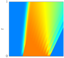
Refer to caption
Refer to caption
Refer to caption
Refer to caption
Refer to caption
Refer to caption
Refer to caption
Refer to caption
Refer to caption
Refer to caption
Refer to caption
Refer to caption
Figure 2: constant kernel γη1χ(0,1)(η1)\gamma\equiv\eta^{-1}\chi_{(0,1)}(\cdot\eta^{-1}) for x𝑥x\in\mathbb{R}, initial datum q014+12χ[0.5,0.5]subscript𝑞01412subscript𝜒0.50.5q_{0}\equiv\tfrac{1}{4}+\frac{1}{2}\chi_{[-0.5,0.5]}, first column: Nonlocal in the solution, V(1)2V\equiv(1-\cdot)^{2}, second column: Nonlocal in the velocity, V=(1)2,V=(1-\cdot)^{2}, third column: nonlocal in the solution, V()=1()2𝑉1superscript2V(\cdot)=1-(\cdot)^{2}, last column: Nonlocal in the velocity, V()=1()2𝑉1superscript2V(\cdot)=1-(\cdot)^{2}. Top row: η=101𝜂superscript101\eta=10^{-1}, middle row: η=102𝜂superscript102\eta=10^{-2} and bottom row: η=103𝜂superscript103\eta=10^{-3}, Colorbar: 000\ Refer to caption 11\,1
Refer to caption
Refer to caption
Refer to caption
Refer to caption
Figure 3: Same setup as in Figs. 1 to 2. Top row: constant kernel, bottom row: exponential kernel, left column: convex velocity V(1)2V\equiv(1-\cdot)^{2}, right column: concave velocity V1()2𝑉1superscript2V\equiv 1-(\cdot)^{2}, solid line: η=101𝜂superscript101\eta=10^{-1}, dashed-dotted: η=102𝜂superscript102\eta=10^{-2} and dashed: η=103𝜂superscript103\eta=10^{-3}, purple and red: nonlocal in velocity, yellow and blue: nonlocal in solution.

7 Conclusions and future work

In this contribution we have studied the convergence to the local entropy solutions when the nonlocal operator does not act on the solution itself but on the velocity. We have established for the exponential kernel and a variety of velocities functions the convergence to the local entropy solution. Moreover, for monotone datum and arbitrary kernels, we obtain this convergence as well. This motivates to study several open problems: 1) Does the convergence generally hold? It seems like the nonlocal averaging over the velocity behaves somewhat more reasonable as it conserves monotonicity, etc., however, on the other hand the results are not as general as in [16]. In our convergence analysis we use a specific strictly convex entropy depending on the velocity. This choice of entropy requires the velocity’s derivative to be nonzero, and restricts the result. Is there another entropy which does not require this assumption and can we thus generalize the result? 2) In a recent preprint, the results for the singular limit problem nonlocal in the solution could be generalized to a variety of other (physical relevant) kernels [40, 17] and it would be important to understand whether this is also possible in the nonlocal in the velocity case. 3) Can we obtain the same results when considering instead of a conservation law a balance law with nonlinear right hand side? 4) In the case of a symmetric kernel, the solutions are not even uniformly bounded with respect to the nonlocal parameter. However, it seems that convergence in a weak sense yet to be determined might still hold and would give an even more general convergence result. 5) Control and optimal control in the singular limit case.

Acknowledgments

Lukas Pflug thanks for the support by the Collaborative Research Centre 1411 “Design of Particulate Products” (Project-ID 416229255). Jan Friedrich was supported by the German Research Foundation (DFG) under grant HE 5386/18-1, 19-2, 22-1, 23-1 and Simone Göttlich under grant GO 1920/10-1.

References

  • [1] A. Aggarwal, R. Colombo, and P. Goatin, Nonlocal systems of conservation laws in several space dimensions, SIAM Journal on Numerical Analysis, 53 (2015), pp. 963–983.
  • [2] M. Aĭzerman, E. Bredihina, S. Černikov, F. Gantmaher, I. Gelfand, S. Gelfer, D. Harazov, M. Kadec, J. Korobeĭnik, M. Kreĭn, O. Oleĭnik, I. Pyateckiĭ-Šapiro, M. Subhankulov, K. Temko, and A. Tureckiĭ, Seventeen Papers on Analysis, American Mathematical Society, 1963.
  • [3] P. Amorim, R. Colombo, and A. Teixeira, On the numerical integration of scalar nonlocal conservation laws, ESAIM: Math. Modelling and Numerical Analysis, 49 (2015), pp. 19–37.
  • [4] D. Armbruster, D. Marthaler, C. Ringhofer, K. Kempf, and T.-C. Jo, A continuum model for a re-entrant factory., Operations Research, 54 (2006), pp. 933–950, http://dblp.uni-trier.de/db/journals/ior/ior54.html#ArmbrusterMRKJ06.
  • [5] A. Bayen, J. Friedrich, A. Keimer, L. Pflug, and T. Veeravalli, Modeling multilane traffic with moving obstacles by nonlocal balance laws, SIAM Journal on Applied Dynamical Systems, 21 (2022), pp. 1495–1538, https://doi.org/10.1137/20M1366654.
  • [6] F. Betancourt, R. Bürger, K. Karlsen, and E. Tory, On nonlocal conservation laws modelling sedimentation, Nonlinearity, 24 (2011), p. 855.
  • [7] S. Blandin and P. Goatin, Well-posedness of a conservation law with non-local flux arising in traffic flow modeling, Numerische Mathematik, 132 (2016), pp. 217–241.
  • [8] A. Bressan, Hyperbolic Systems of Conservation Laws, Oxford University Press, Oxford, 2000.
  • [9] A. Bressan and W. Shen, On traffic flow with nonlocal flux: a relaxation representation, Archive for Rational Mechanics and Analysis volume, 237 (2020).
  • [10] A. Bressan and W. Shen, Entropy admissibility of the limit solution for a nonlocal model of traffic flow, Communications in Mathematical Sciences, 19 (2021), pp. 1447–1450.
  • [11] C. Chalons, P. Goatin, and L. Villada, High-order numerical schemes for one-dimensional nonlocal conservation laws, SIAM Journal on Scientific Computing, 40 (2018), pp. A288–A305, https://doi.org/10.1137/16M110825X.
  • [12] F. Chiarello, J. Friedrich, P. Goatin, S. Göttlich, and O. Kolb, A non-local traffic flow model for 1-to-1 junctions, European Journal of Applied Mathematics, (2019), pp. 1–21.
  • [13] F. Chiarello and P. Goatin, Global entropy weak solutions for general non-local traffic flow models with anisotropic kernel, ESAIM: Math. Modelling and Numerical Analysis, 52 (2018), pp. 163–180.
  • [14] F. A. Chiarello, J. Friedrich, P. Goatin, and S. Göttlich, Micro-macro limit of a nonlocal generalized Aw-Rascle type model, SIAM Journal on Applied Mathematics, 80 (2020), pp. 1841–1861.
  • [15] F. A. Chiarello and P. Goatin, Non-local multi-class traffic flow models, Networks & Heterogeneous Media, 14 (2019), p. 371.
  • [16] G. M. Coclite, J.-M. Coron, N. De Nitti, A. Keimer, and L. Pflug, A general result on the approximation of local conservation laws by nonlocal conservation laws: The singular limit problem for exponential kernels, Accepted in Annales de l’Institut Henri Poincaré C, Analyse non linéaire, (2022).
  • [17] M. Colombo, G. Crippa, E. Marconi, and L. Spinolo, Nonlocal traffic models with general kernels: singular limit, entropy admissibility, and convergence rate, (2022).
  • [18] M. Colombo, G. Crippa, E. Marconi, and L. V. Spinolo, Local limit of nonlocal traffic models: Convergence results and total variation blow-up, Annales de l’Institut Henri Poincaré C, Analyse non linéaire, 38 (2021), pp. 1653–1666.
  • [19] M. Colombo, G. Crippa, and L. Spinolo, On the singular local limit for conservation laws with nonlocal fluxes, Archive for Rational Mechanics and Analysis volume, 233 (2019), p. 1131–1167.
  • [20] R. Colombo, M. Garavello, and M. Lécureux-Mercier, A class of nonlocal models for pedestrian traffic, Mathematical Models and Methods in Applied Sciences, 22 (2012), p. 1150023.
  • [21] R. Colombo and M. Lécureux-Mercier, Nonlocal crowd dynamics models for several populations, Acta Mathematica Scientia, 32 (2012), pp. 177–196.
  • [22] J.-M. Coron, M. Kawski, and Z. Wang, Analysis of a conservation law modeling a highly re-entrant manufacturing system, Disc. Contin. Dyn. Syst. Ser. B, 14 (2010), pp. 1337–1359, https://doi.org/10.3934/dcdsb.2010.14.1337, http://dx.doi.org/10.3934/dcdsb.2010.14.1337.
  • [23] G. Crippa and M. Lécureux-Mercier, Existence and uniqueness of measure solutions for a system of continuity equations with non-local flow, Nonlinear Differential Equations and Applications NoDEA, 20 (2013), pp. 523–537.
  • [24] C. De Filippis and P. Goatin, The initial–boundary value problem for general non-local scalar conservation laws in one space dimension, Nonlinear Analysis, 161 (2017), pp. 131–156.
  • [25] C. De Lellis, F. Otto, and M. Westdickenberg, Minimal entropy conditions for burgers equation, Quarterly of applied mathematics, 62 (2004), pp. 687–700.
  • [26] R. Eymard, T. Gallouët, and R. Herbin, Finite volume methods, Handbook of numerical analysis, 7 (2000), pp. 713–1018.
  • [27] J. Friedrich, S. Göttlich, and M. Osztfalk, Network models for nonlocal traffic flow, ESAIM: Mathematical Modelling and Numerical Analysis, 56 (2022), pp. 213–235.
  • [28] J. Friedrich, O. Kolb, and S. Göttlich, A godunov type scheme for a class of LWR traffic flow models with non-local flux, Networks & Heterogeneous Media, 13 (2018), p. 531.
  • [29] P. Goatin and E. Rossi, A multilane macroscopic traffic flow model for simple networks, SIAM Journal on Applied Mathematics, 79 (2019), pp. 1967–1989.
  • [30] P. Goatin and E. Rossi, Well-posedness of IBVP for 1D scalar non-local conservation laws, ZAMM - Journal of Applied Mathematics and Mechanics / Zeitschrift für Angewandte Mathematik und Mechanik, 99 (2019).
  • [31] P. Goatin and S. Scialanga, Well-posedness and finite volume approximations of the LWR traffic flow model with non-local velocity, Networks and Hetereogeneous Media, 11 (2016), pp. 107–121.
  • [32] E. Godlewski and P.-A. Raviart, Hyperbolic systems of conservation laws, Ellipses, 1991.
  • [33] X. Gong and M. Kawski, Weak measure-valued solutions of a nonlinear hyperbolic conservation law, SIAM Journal on Mathematical Analysis, 53 (2021), pp. 4417–4444.
  • [34] B. Greenshields, W. Channing, H. Miller, et al., A study of traffic capacity, in Highway research board proceedings, vol. 1935, National Research Council (USA), Highway Research Board, 1935.
  • [35] M. Gugat, A. Keimer, G. Leugering, and Z. Wang, Analysis of a system of nonlocal conservation laws for multi-commodity flow on networks, Networks & Het. Media, 10 (2015), pp. 749–785, https://doi.org/10.3934/nhm.2015.10.749, http://aimsciences.org/journals/displayArticlesnew.jsp?paperID=11749.
  • [36] A. Keimer and L. Pflug, Existence, uniqueness and regularity results on nonlocal balance laws, Journal of Differential Equations, 263 (2017), pp. 4023–4069.
  • [37] A. Keimer and L. Pflug, On approximation of local conservation laws by nonlocal conservation laws, Journal of Mathematical Analysis and Applications, 475 (2019), pp. 1927 – 1955.
  • [38] A. Keimer and L. Pflug, Discontinuous nonlocal conservation laws and related discontinuous ODEs – existence, uniqueness, stability and regularity, (2021), https://arxiv.org/abs/2110.10503.
  • [39] A. Keimer and L. Pflug, On the singular limit problem for a discontinuous nonlocal conservation law, submitted, (2022).
  • [40] A. Keimer and L. Pflug, On the singular limit problem for nonlocal conservation laws: A general approximation result for kernels with fixed support, submitted, (2022).
  • [41] A. Keimer, L. Pflug, and M. Spinola, Existence, uniqueness and regularity of multi-dimensional nonlocal balance laws with damping, Journal of Mathematical Analysis and Applications, 466 (2018), pp. 18 – 55, https://doi.org/https://doi.org/10.1016/j.jmaa.2018.05.013, http://www.sciencedirect.com/science/article/pii/S0022247X18304062.
  • [42] A. Keimer, L. Pflug, and M. Spinola, Nonlocal balance laws: Theory of convergence for nondissipative numerical schemes, submitted, (2018).
  • [43] A. Keimer, L. Pflug, and M. Spinola, Nonlocal scalar conservation laws on bounded domains and applications in traffic flow, SIAM SIMA, 50 (2018), pp. 6271–6306.
  • [44] A. Keimer, M. Singh, and T. Veeravalli, Existence and uniqueness results for a class of nonlocal conservation laws by means of a lax–hopf-type solution formula, Journal of Hyperbolic Differential Equations, 17 (2020), pp. 677–705.
  • [45] P. Kloeden and T. Lorenz, Nonlocal multi-scale traffic flow models: analysis beyond vector spaces, Bulletin of Mathematical Sciences, 6 (2016), pp. 453–514.
  • [46] S. Kružkov, First order quasilinear equations in several independent variables, Mathematics of the USSR-Sbornik, 10 (1970), p. 217.
  • [47] Y. Lee, Thresholds for shock formation in traffic flow models with nonlocal-concave-convex flux, Journal of Differential Equations, 266 (2019), pp. 580 – 599.
  • [48] G. Leoni, A first course in Sobolev spaces, vol. 105 of Graduate Studies in Mathematics, American Mathematical Society, Providence, RI, 2009.
  • [49] T. Lorenz, Nonlocal hyperbolic population models structured by size and spatial position: Well-posedness, Discrete & Continuous Dynamical Systems-B, 24 (2019), p. 4547.
  • [50] T. Lorenz, Viability in a non-local population model structured by size and spatial position, Journal of Mathematical Analysis and Applications, 491 (2020), p. 124249.
  • [51] O. Oleinik, Discontinuous solutions of non-linear differential equations, Uspekhi Mat. Nauk, 12 (1957), pp. 3–73.
  • [52] L. Pflug, T. Schikarski, A. Keimer, W. Peukert, and M. Stingl, eMoM: Exact method of moments—nucleation and size dependent growth of nanoparticles, Computers & Chemical Engineering, 136 (2020), p. 106775.
  • [53] B. Piccoli, N. Duteil, and E. Trélat, Sparse control of Hegselmann–Krause models: Black hole and declustering, SIAM Journal on Control and Optimization, 57 (2019), pp. 2628–2659.
  • [54] E. Rossi, J. Weißen, P. Goatin, and S. Göttlich, Well-posedness of a non-local model for material flow on conveyor belts, ESAIM: Mathematical Modelling and Numerical Analysis, 54 (2020), pp. 679–704.