Describing Sets of Images with Textual-PCA

Abstract

We seek to semantically describe a set of images, capturing both the attributes of single images and the variations within the set. Our procedure is analogous to Principle Component Analysis, in which the role of projection vectors is replaced with generated phrases. First, a centroid phrase that has the largest average semantic similarity to the images in the set is generated, where both the computation of the similarity and the generation are based on pretrained vision-language models. Then, the phrase that generates the highest variation among the similarity scores is generated, using the same models. The next phrase maximizes the variance subject to being orthogonal, in the latent space, to the highest-variance phrase, and the process continues. Our experiments show that our method is able to convincingly capture the essence of image sets and describe the individual elements in a semantically meaningful way within the context of the entire set. Our code is available at: https://github.com/OdedH/textual-pca.

1 Introduction

Given a set of images with a common theme, it seems to be extremely easy for humans to identify and describe the common theme. While computer algorithms can identify in-set and out-of-set images using anomaly detection methods Schölkopf et al. (1999); Golan and El-Yaniv (2018), describing the common theme seems more challenging.

Captioning methods Mao et al. (2014); Li et al. (2020); Tewel et al. (2022b); Li et al. (2022) are extremely effective in describing single images. However, one cannot directly employ such a method to the mean image representation, in hope of describing a set of images. Since image captioning engines are trained to be specific and not to provide general terms, the resulting captions would not be generic enough. For example, images of people are described by image captioning methods as “man”, “woman”, “child”, etc., and not by generic terms, such as “person”. To create a representation of an image set, one has to employ higher-level themes. Unable to do so, image captioning methods output non-grammatical phrases, which include, for example, phrases such as “cat dog” for sets that contain both pet species.

Our first contribution is to retool the BLIP Li et al. (2022) image captioning tool to perform the task of image-set captioning. This is done through modifying the autoregressive process of BLIP without retraining the underlying network. WordNet Miller (1995) is used to manipulate the likelihood of words by reducing the likelihood of hyponyms (specific terms) and increasing the likelihood of shared hypernyms (more generic terms).

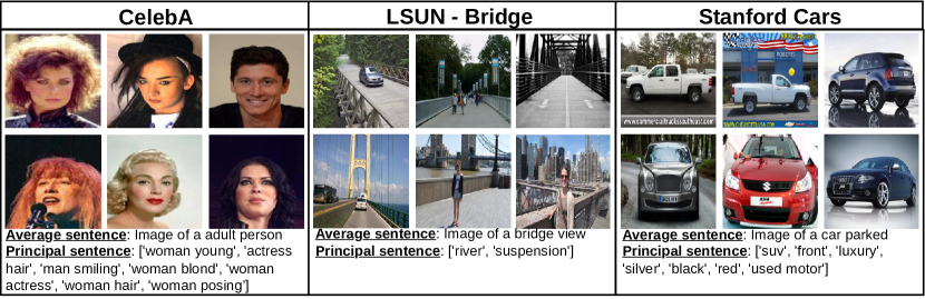
Figure 1: Examples of our textual PCA. For each dataset, we present an average phrase that describes the image set and the principal phrases, i.e., phrases that maximize the variance of the image-to-text matching score subject to being mutually orthogonal in the embedding space.

Once a common theme is generated for the image set, we seek to identify the directions of variation within the set. This way, we can position the set elements in the context of the entire set. For example, staying with the example of images of persons, the images can vary by pose, age, hair style, facial expression, etc.

Motivated by the PCA method, we seek to find the phrase whose visual-language similarity to the images of the set has the highest variance. Then, once again following PCA, we recover a phrase that maximizes the variance among all phrases that are orthogonal to the first phrase in the textual embedding space.

Our second contribution is, therefore, the ability to extract different phrases that capture directions of semantic variability in the image set. This is also done by retooling BLIP. In this case, the likelihood of the next token combines three terms: (i) the likelihood assigned by BLIP, (ii) a term that maximizes the variance of the similarity between the resulting phrase and the images of the input set, and (iii) an orthogonality term that distances the generated phrase from the previously found phrases.

Our textual PCA method seems to be highly suitable for describing sets of images in an intuitive way that combines the general theme with the modes of variation. Consider, for example, Fig. 1. The average phrase clearly depicts that CelebA is a dataset featuring images of adult persons or that LSUN-Bridge contains images of bridges. From the principal phrases we can learn about the traits of the dataset. For example, hair varies considerably in CelebA, and the LSUN-Bridge images differ mainly in the type of the bridge (suspension) or whether it crosses a river.

We evaluate our method on multiple datasets, including existing image datasets, such as CelebA, LSUN, and ImageNet, and on sets of images obtained by applying clustering methods to large image collections. We also show that the obtained projections are more informative than the baselines in predicting attributes in CelebA. Finally, in lineup-type experiments, we show that the projections we create provide enough information for users to identify the images out of the set.

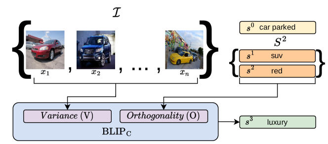
Figure 2: An overview of our approach to generate principal phrases by modifying BLIP’s caption head. The first step is to create an average phrase, ’car parked’ that captures the common features of the set of images $\mathcal{I}$. Then, during the auto-regression process, we consider two types of operators: (i) $\operatorname{V}$ for maximizing the variance over the images, and (ii) $\operatorname{O}$ for generating phrases that are orthogonal to the previous phrases (e.g., ‘suv’, ‘red’). The result is a novel phrase ‘luxury’ that describes the car’s pricing.

2 Related work

Some of the earliest deep learning attempts in image captioning relied on RNNs with attention Mao et al. (2014); Klein et al. (2014); Xu et al. (2015), while more recent approaches apply spatial reasoning via graphs Yao et al. (2018); Kipf and Welling (2017), adapt to multi-image processing Braude et al. (2022), and handle multi-modal input Schwartz et al. (2019). Annotations by humans are used to train most of the current captioning methods. As human references cannot account for every possible scene, other approaches rely more on web-scale unsupervised image-text datasets Zhang et al. (2021); Devlin et al. (2018); Li et al. (2020). In these approaches, smaller datasets annotated by humans are used as final fine-tuning. Captions based on human annotations can enhance correspondence with human annotators. There is, however, a tendency for them to be repetitive and not particularly informative.

Recently, several methods that employ web-scale training data directly have been suggested. The first method, ZeroCap, employs CLIP Radford et al. (2021), a prominent web-scale image-text matching model, to guide a pre-trained language model, GPT-2, to caption images Tewel et al. (2022b, a) without performing any training (“zero-shot”). MAGIC Su et al. (2022), is another zero-shot method for image captioning that skews the next-token distribution of a GPT-2 language model to match a given image, based on the CLIP score. Unlike ZeroCap, no gradient updates are applied. BLIP Li et al. (2022) applies conventional training (not zero-shot) and jointly learns an image-text metric with a contrastive loss and a caption decoder head.

Also relevant to our work are causality frameworks that study concept discovery, such as TCAV Kim et al. (2018) and CaCE Goyal et al. (2019). By intervening on labeled concepts, these approaches study causal effects. However, they require labeled data. Although expertise can be acquired to identify the underlying structure of a problem, the process is still contaminated by human bias. In contrast to these approaches, ours does not require supervision.

The discovery of visual concepts is also a subject of research. An intuitive approach involves clustering according to segmented regions Ghorbani et al. (2019). A Shapley theorem-inspired method is described in subsequent work Yeh et al. (2019). In a StyleGAN model, latent variables that control the semantic properties of images are disentangled Karras et al. (2019). Consequently, a disentangled StyleSpace was proposed for finding the attributes that determine classification Lang et al. (2021). Variational auto-encoders can also be used to reveal concepts used to predict classes Gat et al. (2021). These methods involve finding visual concepts, whereas our approach involves finding textual concepts that describe visual content. This shift is not trivial; in existing works, the meaning of each direction is assigned by human observers, based on manually inspecting samples, and not all directions can be easily described.

3 Method

Our approach is analogous to Principal Component Analysis (PCA), in which the projection directions are replaced by generated phrases, Fig. 2. PCA identifies the vectors that best fit the data, in terms of Euclidean distance between each data point and its reconstructed vector. It can be equivalently defined as finding directions that maximize the variance of the projected data. The principal vectors are, therefore, directions in which data varies, making them informative. This makes them highly useful for data analyses and dimensionality reduction. These vectors are extracted as mutually orthogonal vectors, in order to capture different directions, and for the projections to span the entire data set.

While PCA can be applied to embedded image vectors, we find that it lacks semantic meaning. In this work, we propose Textual-PCA. Formally, our goal is to create a average phrase $s^{0}$ and a sequence of principal phrases $S^{l}=\langle s^{1},\dots s^{l}\rangle$, where $l$ is the number of principal phrases. The phrases are aimed to be a concise set that describes a set of images $\mathcal{I}=\{x_{1},\ldots,x_{n}\}$, where $n$ is the number of images. The phrase $s^{0}$ captures common traits in $\mathcal{I}$, and the rest capture different modes of variability. In the following sections we discuss how we find fluent principal phrases.

A principal phrase is created by finding a textual direction that captures semantic variance within an image set. Throughout our process, we employ the multi-modal BLIP model Li et al. (2022), which provides textual and image encoders ($E_{T}$ and $E_{I}$, respectively), an image-text metric ($\operatorname{BLIP}_{\text{M}}$), and a captioning head ($\operatorname{BLIP}_{\text{C}}$).

Given the set of images $\mathcal{I}$, we start the process with the generation of the average phrase $s^{0}$. This phrase captures the common attributes of all images in the set. As the first step of generating the average phrase, we average the image representations, $\bar{x}=\frac{1}{n}\sum_{x_{i}\in\mathcal{I}}E_{I}(x_{i})$. We then use $\bar{x}$ to initialize the auto-regressive BLIP’s captioning head,

$$s^{0}_{t+1}=\operatorname{BLIP}_{\text{C}}(s^{0}_{t},\bar{x})\,,$$ (1)

where $s^{0}_{t}$ is the average phrase of length $t$.

3.1 Generating the average phrase

In the average phrase, we aim for the most generic attributes. For instance, we prefer to increase the potential of the “church” token over the more specific “cathedral” token, if both of them are top tokens. However, image captioning models are trained on specific captions, and, as a result, tend to be very specific.

We, therefore, intervene in the BLIP auto-regressive generation process by manipulating the likelihood of each token. Based on the WordNet graph Miller (1995), we aggregate specific terms that have similar meanings into more general terms.

Our algorithm only considers the top 12 most probable tokens and zero out the rest. This value was determined early in the development process and kept unmodified to obtain all results. Captioning models tend to describe items at a certain level dictated by the training data, i.e., use ‘cat’ and not ‘mammal’ or ‘Persian cat.’ This is probably dictated by the basic level at which items are often perceived Rosch et al. (1976). Since the replacement method relies on tokens in the top-tokens list, the average sentence is more specific (e.g., ‘cat’ and not ‘mammal’). We then iterate across all candidate tokens in the order of their likelihood.

For each candidate token $t$, we consider, among all other tokens, the set $A_{1}$ that contains tokens $r$ such that $r$ is an immediate “is-a” ancestor of $t$ (a direct hypernym). In this set, we consider the token $r$ with the higher probability, and add the probability assigned to $t$ to the probability associated with $r$, while zeroing the probability of $t$.

If the set $A_{1}$ is empty, we consider the set $A_{2}$ that contains tokens $r$ that are direct hyponyms of $t$. We add the probabilities of all $r\in A_{2}$ to that of $t$, and zero the probabilities of these hyponyms.

Finally, if set $A_{2}$ is also empty, we consider the set $A_{3}$ that contains all tokens $r$ among the tokens such that $t$ and $r$ have a shared direct hyponym $q$. Among the set $A_{3}$, we select token $r$ with the highest probability and add token $q$ to the set of candidate tokens with a probability that sums the probabilities of both $t$ and $r$. The probabilities of these two tokens are then zeroed.

Two concrete examples, based on real images are: (i) the token $t$=‘sofa’. $A_{1}$ and $A_{2}$ are empty. Two other probable words in $A_{3}$={‘chair’, ‘bench’} share the same hypernym $q$=‘seat’. The probability of r=‘chair’ is higher than ’bench’, we update $\text{prob}(q)=\text{prob}(r)+\text{prob}(t)$, $\text{prob}(r)=\text{prob}(t)=0$, where prob is the likelihood of the given token. (ii) Another example for the word $t$=’salad’, $A_{1}$={‘dish’}, which is the immediate hypernym of t. $A_{3}$={‘pasta’, ‘soup’, ‘curry’…} those words share the same hypernym ‘dish’ and are probable tokens. In this scenario, the probability of the token $t$=‘salad’ would add to the likelihood of the token $r$=‘dish’ from $A_{1}$, i.e., $\text{prob}(r)=\text{prob}(r)+\text{prob}(t)$, and $\text{prob}(t)=0$.

3.2 Generating the principal phrases

The next principal phrases, which capture variance, are also generated with the $\operatorname{BLIP}_{\text{C}}$ auto-regressive process. We initialize the captioning head again with $\bar{x}$. During the auto-regressive process, we modify the next token potentials with two terms: (i) $\operatorname{V}$, which maximizes the variance of the generated phrase with the images, and (ii) $\operatorname{O}$, which is responsible for maximizing orthogonality with the previous phrases (WordNet is not used).

Let $\hat{p}_{t,k}^{i}$ be the potential of the $i$-th principle phrase of length $t$, $t-1$ of which were already set, to have token $k$ at position $t$,

$$\hat{p}_{t,k}^{i}\propto\exp(p_{t,k}^{i}+\lambda_{v}\operatorname{V}(s_{t,k}^{i},\mathcal{I})-\lambda_{o}\operatorname{O}(s_{t,k}^{i},S^{i-1})),$$

where $p_{t,k}^{i}$ is the original distribution of BLIP’s captioning head, and $s_{t,k}^{i}$ is the $i$-th principle phrase after $t-1$ steps, with token $k$ at location $t$. $\lambda_{v},\lambda_{o}\in\mathbb{R}$ are hyperparameters. We compute $\hat{p}_{t,k}^{i}$ only for the 1000 most likely tokens (those with the highest $p_{t,k}^{i}$), since the potential of the remaining tokens is usually close to zero.

We define the variance operator $\operatorname{V}$ as the sum of the BLIP’s matching scores between the token $s_{t,k}^{i}$ and an image in the set $x\in\mathcal{I}$ minus the average BLIP’s matching score, i.e.,

$$\operatorname{V}\left(s_{t,k}^{i},\mathcal{I}\right)=\sum_{x\in\mathcal{I}}(\operatorname{BLIP}_{\text{M}}(s_{t,k}^{i},x)-\mu(s_{t,k}^{i}))^{2},$$

where $\mu(s_{t,k}^{i})=\frac{1}{n}\sum_{x\in\mathcal{I}}\operatorname{BLIP}_{\text{M}}(s_{t,k}^{i},x)$, and $\operatorname{BLIP}_{\text{M}}$ is a BLIP’s matching score. Prior to calculating this matching score, we subtract the embedding of the average phrase $s_{0}$ from the generated phrase embedding.

The orthogonality term $\operatorname{O}$ serves to emphasize novel phrases that encapsulate the broad set of factors that define an image set, by encouraging orthogonality between the current phrase potential and all previous phrases in BLIP’s phrase embedding space

$$\operatorname{O}\left(s_{t,k}^{i},\mathcal{S}^{i-1}\right)=\sum_{s^{j}\in\mathcal{S}^{i-1}}E_{T}(s_{t,k}^{i})^{\top}E_{T}(s^{j}),$$ (2)

where $E_{T}$ is BLIP’s textual encoder. This way, the principle components do not repeat the description of the set, despite conditioning the generator on the same mean vector $\bar{x}$.

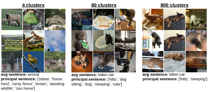
Figure 3: Hierarchical clustering of COCO at different granularity levels. As the clusters get smaller, i.e., with more clusters, they become more homogenous and the principal phrases become more specific.

Method	Named Datasets	COCO	ImageNet
Most Frequent Words	0.808 $\pm$ 0.14	0.835 $\pm$ 0.37	0.636 $\pm$ 0.16
ZeroCap+PCA (CLIP space)	1.068 $\pm$ 0.43	0.885 $\pm$ 0.80	0.676 $\pm$ 0.30
ZeroCap+KMeans (CLIP space)	1.128 $\pm$ 0.47	1.077 $\pm$ 1.49	0.586 $\pm$ 0.33
MAGIC+PCA (CLIP space)	1.035 $\pm$ 0.34	0.891 $\pm$ 0.78	0.666 $\pm$ 0.26
MAGIC+KMeans (CLIP space)	1.270 $\pm$ 0.56	1.049 $\pm$ 1.14	0.685 $\pm$ 0.36
ZeroCap+PCA (BLIP space)	1.290 $\pm$ 0.40	1.001 $\pm$ 0.89	0.992 $\pm$ 0.33
ZeroCap+KMeans (BLIP space)	1.225 $\pm$ 1.13	1.225 $\pm$ 1.32	0.712 $\pm$ 0.27
MAGIC+PCA (BLIP space)	1.128 $\pm$ 0.19	1.004 $\pm$ 0.91	0.744 $\pm$ 0.31
MAGIC+KMeans (BLIP space)	1.073 $\pm$ 0.4	1.051 $\pm$ 1.02	0.706 $\pm$ 0.43
Ours	1.515 $\pm$ 0.65	1.261 $\pm$ 1.56	1.095 $\pm$ 0.47

Table 1: Variance in the BLIP space, averaged, per image, across all principle phrases. Shown are the mean$\pm$ Standard Deviation in each group of image sets.

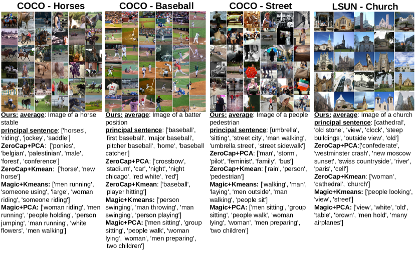
Figure 4: Four image sets: COCO-horses, COCO-baseball, and COCO-Street (names were assigned by us) obtained by clustering COCO, a large visual dataset, and LSUN-Church. For each image set we present the average phrase and principal phrases generated by our method (underlined). For comparison, we present four baselines: ZeroCap+PCA, ZeroCap+KMeans, MAGIC+PCA, and MAGIC+KMeans, obtained in BLIP space.

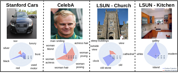
Figure 5: Sample radar plots, in which the value of the projection to the principle phrases are depicted. In blue we show positive correlation and in red negative correlation.

4 Results

In all experiments, we set the hyperparameter $\lambda_{v}=5$ and $\lambda_{o}=10$. These values were determined early on in the development process and kept unmodified for obtaining all results.

Evaluation is done on datasets covering a variety of objects and settings (i.e., Named Datasets). CelebA Yang et al. (2015) is a large-scale dataset of faces. LSUN Yu et al. (2015) contains ten different scene categories, from which we use the images of bridges, churches, and kitchens. The Stanford cars dataset contains different types of vehicles.

The first 20 categories of ImageNet Deng et al. (2009) were also used.

We also employ sets that were obtained by hierarchically clustering COCO Lin et al. (2014) with an agglomerative algorithm in the CLIP embedding space. We cluster until we obtain 80 clusters. This number was selected since there is a small hinge around 80 in the graph depicting the number of clusters vs. the clustering error. Second, with 80 clusters, large enough clusters are starting to form. Fig. 3 demonstrates the level of specificity obtained for three levels of clustering. With 4 clusters, one can see a cluster of animals; with 80 clusters, a cluster of cats exists, and with 800 clusters, a subset of the cats with less variation is obtained. Notably, to describe datasets with varying themes, clustering as a first step is a practical technique.

For computational efficiency, from large datasets, such as CelebA or LSUN and some COCO clusters, we sampled 500 images (each) as the working set.

baselines  Our baselines consider sets of vectors in the embedding space of BLIP and then transcribe these into phrases. The sets of vectors are obtained by one of two methods, which are applied to the set of all embedding vectors extracted, using the image encoder, for a given set of images.

The first method is PCA, which uses Singular Value Decomposition, and the second method is cosine k-means clustering, which was selected since embedding methods have a norm of one. In the case of k-means, the centroids of each cluster are used as the extracted components.

Note that K-means and PCA are related with relaxation assumptions Zha et al. (2001).

Turning these sets of principle vectors into phrases is done through either the ZeroCap method Tewel et al. (2022b) or using MAGIC Su et al. (2022). Since our method operates in the BLIP encoding space, we created a version of both ZeroCap and MAGIC that are BLIP-based. The results of the unmodified baselines when using CLIP embedding space are also presented.

We also attempted to use BLIP’s captioning head to generate text from the principal vectors. However, despite considerable effort, the generation collapsed into the model’s default caption. This is most likely due to the sensitivity of the captioning head to distribution changes, i.e., the distribution of PCA vectors differs considerably from the encoding of single images that BLIP was trained on.

We further evaluate a naive baseline of most frequent words. We used BLIP captioning head to generate captions for the images in the set. Then, we created phrases based on the most frequent words.

Method	CLIP space	BLIP space
ZeroCap+PCA	0.840	0.846
ZeroCap+KMeans	0.813	0.823
MAGIC+PCA	0.849	0.840
MAGIC+KMeans	0.852	0.829
Ours	0.858	0.862

Table 2: Test accuracy scores for predicting annotated attributes of CelebA dataset, using a simple MLP over the projected values (similarities between the principle phrases and the image).

Quantitative Results 

Given a set of principal phrases $S$, and a set of images $\mathcal{I}$, the variability score measures

$$|S|^{-1}|\mathcal{I}|^{-1}\sum_{s\in S}\sum_{x\in\mathcal{I}}(E_{T}(s)^{\top}E_{I}(x)-\mu_{s})^{2},$$ (3)

where $\mu_{s}=|\mathcal{I}|^{-1}\sum_{x\in\mathcal{I}}(E_{T}(s)^{\top}E_{I}(x))$.

The results are presented in Tab. 1. We find that our approach outperforms all baselines. Note that since PCA in the embedding space maximizes the variance there, any variance lost is a result of translating the principal directions into coherent phrases and back into BLIP space vectors.

In addition to measuring variance, we also ask to test to what extent principal phrases capture natural traits of the dataset. To this aim, we use the CelebA dataset, a dataset of portrait images of celebrities, since attribute labels for it are available. In CelebA, 40 facial traits are annotated (e.g. hair color, eyeglasses). These are attributes containing semantic information that is not explicitly exposed at the phrase generation stage.

We consider the generated principal phrases $S_{m}$ for each method $m$, and embed those phrases back into BLIP, i.e., for each $s\in S_{m}$, we compute $E_{T}(s)$. Similarly to PCA, we project each image $x$ of the image set $\mathcal{I}$ by computing $E_{T}(s)^{\top}E_{I}(x)$. Aggregating over all $s\in S_{m}$, we represent each image $x$ as one vector for each method $m$. Using basic MLPs with one hidden layer, we then predict the CelebA datasets attributes from these vectors.

Prediction accuracy on the CelebA test set is reported in Tab. 2. Evidently, our approach achieves a higher test accuracy score than all baselines.

Qualitative results  Sample results for our method can be found in Fig. 1,3. The baselines are not shown, but they are not competitive. Fig. 4 provides our results for additional datasets, as well as those of the baseline methods. Comparing the most frequent words baseline on the Cars dataset, our method (variance score of $0.963$) extracts: ’suv’, ’front’, ’luxury’, ’silver’, ’black’, ’red’, ’used motor’. Most frequent words (variance score of 0.643) extracts: ’parked’, ’car’, ’front’, ’lot’, ’parking’, ’black’, ’red’. Shown are the results on COCO clusters, which are less homogenous than human-created datasets, as well as on the LSUN-Church dataset. Evidently, the average phrase and the principal phrases produced by our method are related to the theme of the dataset.

Our method extracts multiple relevant attributes. It characterized Churches by structural attributes, such as having a clock or steeple, by their age, or by purpose (the cathedrals attribute). Interestingly, in the horse-related cluster, there is a quantity-related term, horses. In COCO-Baseball the phrases refer to the role of the person (‘baseball pitcher’, ‘baseball catcher’) the league (‘major baseball’) and the location (‘first baseball’ or ‘home’).

The baselines ZeroCap+KMeans and MAGIC+KMeans give a very general description that is similar to an average phrase, while ZeroCap+PCA and MAGIC+PCA return phrases that are not related to the image set. For example, in COCO-horses, ZeroCap+PCA produces ‘conference’ as a principal phrase and MAGIC+PCA ‘white flowers’.

For COCO-Street, all methods identify that many images present a rainy scene and most relate to ‘street’ or ’pedestrian’. The baselines give a more general description of the set, while our method extracts the specific modes of variation. For example, instead of the general term ‘rainy’, we note if an ‘umbrella’ is present in the photo.

	Answered	Of those answered
Method		Correct	Incorrect
ZeroCap+PCA	0.25	0.33	0.67
MAGIC+PCA	0.63	0.07	0.93
Ours	0.98	0.83	0.17

Table 3: Lineup results for matching radar plots with images. Users could decide not to make a choice. The 1st numerical column contains the ratio of questions that the users chose to answer. The other columns depict the success rate out of the answered queries.

Figure 6: An example query from the lineup user study.

User study  To evaluate the usefulness of the principal phrases in describing images in the context of their image set, we conduct a user study in the form of a lineup. For this, we employ a novel radar plot, which marks both positive and negative projections onto the principal phrases, see Fig. 5.

Each user is given a series of radar plots created by the various methods. For each radar plot, the user is asked to select the matching image out of four options, or to check the option “I cannot tell”, see Fig. 6. The $n=20$ users were first trained using sample radar plots created manually.

We compare our method to the two strongest baselines ZeroCap+PCA and MAGIC+PCA, both in BLIP space. The results, listed in Tab.3, show that in almost all cases, the users were willing to identify the matching images for our method, while for other methods, they were more reluctant to do so. Out of the choices made, users were able to select the correct image in far more cases for our method than for the baselines.

Ablation and parameter sensitivity  When generating the average phrase, we aim to generate a general description of the dataset. In order to do so, we use WordNet to aggregate terms to a more general term, as explained 3. Without WordNet, the method produces specific phrases that tend to contain recurrent terms, which are less preferable when describing a dataset, as can be seen in Tab. 4.

Dataset	w/o WordNet	w/ WordNet
CelebA	woman man	adult person
Stanford Cars	car suv	car parked
COCO-Horses	horse horses	horse stable
LSUN-Church	church cathedral	church

Table 4: Average phrases when using or not using Wordnet for aggregating terms. We omit the prompt “Image of a”.

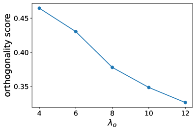
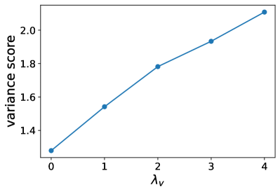
(a)	(b)

Figure 7: Hyperparameter sensitivity. (a) The effect of the hyperparameter $\lambda_{o}$ on the mean orthogonality score of the image sets. (b) The effect of the hyperparameter $\lambda_{v}$ on the mean variance score of the image sets.

The orthogonality coefficient controls the amount of orthogonality between the principal phrases. If we set $\lambda_{o}=0$, the first principal phrase, which maximizes variance, will be repeated over and over, as we empirically confirmed (there is stochasticity in the method).

If we set it to a very large number, for example $\lambda_{o}=1000$, we still receive our original first principal phrase, since the orthogonality of one phrase to itself is 0. However, the following phrases lose all connection to the image set in favor of being orthogonal. For example, for LSUN church we will get: [’cathedral’, ’johns like’, ’overlook sculptures’, ’floppy flags’, ’daytime narrow’, ’sofia framed’, ’gravel’]. For Stanford cars, instead of [’suv’, ’front’, ’luxury’, ’silver’, ’black’, ’red’, ’used motor’] we get [’suv’, ’old monroe’, ’frankfurt’, ’kidney seller’, ’asphalt’, ’poles purple’].

In Fig. 7(a) we quantify how changing $\lambda_{o}$ effects the orthogonality score (Eq. 2). This is shown for the mean score over all datasets discussed in Sec. 4 (Named Datasets, COCO, ImageNet). In these experiments $\lambda_{v}$ is fixed at the default value, and $\lambda_{o}$ varies from its default value of $10$. As can be seen, for a wide range of $\lambda_{o}$ values, the orthogonality score is relatively stable.

The coefficient $\lambda_{v}$ controls the emphasis on maximizing the variance. If we set $\lambda_{v}=0$ we are left with two other constraints: describing the image set, which is done with BLIP’s caption head, and an orthogonality constraint. Therefore, in this case, we obtain meaningful attributes that produce somewhat less variance. As an example, for Stanford Cars, instead of the attributes that maximize and are sorted by variance, [’suv’, ’front’, ’luxury’, ’silver’, ’black’, ’red’, ’used motor’] we get [’silver’, ’front’, ’luxury used’]. Similarly, for CelebA, instead of [’woman young’, ’actress hair’, ’man smiling’, ’woman blond’, ’woman actress’, ’woman hair’, ’woman posing’], we get [’hair hairs’, ’young premiere’, ’man woman’, ’press’, ’hollywood photo’, ’young’, ’man’]. If we set $\lambda_{v}$ to a very large number, $\lambda_{v}=1000$, it will produce the same principal phrase that maximizes variance, since it will overcome orthogonality. For Stanford Cars we now get [’suv truck’] and for CelebA [’female’].

Fig. 7(b) shows how changing $\lambda_{v}$ effects the variance score calculated by Eq. 3. The results are shown for the mean score over all datasets discussed in 4 (Named Datasets, COCO, ImageNet). Despite varying the coefficient over a wide range (the default value we use is 5), the variance remains in a narrow band that outperforms the baseline methods. This includes the case of $\lambda_{v}=0$ discussed above. We, therefore, conclude that having a related text and orthogonal phrases already lead to the desired PCA effect. Adding the variance maximization term further improves results.

5 Discussion and limitations

We identify a few ways in which our results could be extended. First, similarly to other generative tasks, evaluation of the results is not straightforward. Since describing an image set in a way that encompasses both the common theme and the modes of variation is a novel task, there is no established methodology for this evaluation. We believe that the lineup experiments presented demonstrate that humans are able to relate the obtained projections to the images. Given more resources to train human annotators, it would be interesting to obtain human phrases for both the theme and the variation and evaluate the degree to which these would match the method’s results. Second, our method could help create more informative image captions by including the information of the radar plots we present within the generated text. This way, a rich and descriptive captioning, which addresses the common variations from in-set images with a common theme, would be created.

Finally, there is no reason not to apply our method to sets of phrases or paragraphs, by replacing CLIP with a summarization engine, such as those based on transformers Vaswani et al. (2017). Distancing ourselves even further from the current work, we note that with the advent of powerful image generation engines Ramesh et al. (2021) the role that images and text play in our work could be reversed. Images can visually capture the common theme of a set of phrases or paragraphs as well as their modes of variation.

6 Conclusions

Dimensionality reduction methods capture the most significant information of the input vectors using a smaller set of variables. However, these modes are free from semantic constraints and often mix multiple attributes, due to correlations that exist in the data. In this work, we follow in the footsteps of PCA, perhaps the most widely used dimensionality reduction method, and propose a method for extracting orthogonal semantic directions that describe a set of images in the latent space of a vision-language model. First, the “centroid” phrase, which describes the main theme of the set is extracted. Then, the directions with the highest variability in the vision-language similarity to the images of the set are extracted.

Our solution combines the BLIP image captioning model with information derived from the WordNet graph. An extensive set of experiments demonstrates that the obtained list of semantically-orthogonal phrases accurately describes the set of images given as input.

References

- Braude et al. (2022) Tom Braude, Idan Schwartz, Alex Schwing, and Ariel Shamir. 2022. Ordered attention for coherent visual storytelling. In Proceedings of the 30th ACM International Conference on Multimedia.
- Deng et al. (2009) Jia Deng, Wei Dong, Richard Socher, Li-Jia Li, K. Li, and Li Fei-Fei. 2009. Imagenet: A large-scale hierarchical image database. CVPR.
- Devlin et al. (2018) Jacob Devlin, Ming-Wei Chang, Kenton Lee, and Kristina Toutanova. 2018. Bert: Pre-training of deep bidirectional transformers for language understanding. arXiv preprint arXiv:1810.04805.
- Gat et al. (2021) Itai Gat, Guy Lorberbom, Idan Schwartz, and Tamir Hazan. 2021. Latent space explanation by intervention. arXiv preprint arXiv:2112.04895.
- Ghorbani et al. (2019) Amirata Ghorbani, James Wexler, James Y Zou, and Been Kim. 2019. Towards automatic concept-based explanations. NeurIPS.
- Golan and El-Yaniv (2018) Izhak Golan and Ran El-Yaniv. 2018. Deep anomaly detection using geometric transformations. In NeurIPS.
- Goyal et al. (2019) Yash Goyal, Amir Feder, Uri Shalit, and Been Kim. 2019. Explaining classifiers with causal concept effect (cace). arXiv preprint arXiv:1907.07165.
- Karras et al. (2019) Tero Karras, Samuli Laine, and Timo Aila. 2019. A style-based generator architecture for generative adversarial networks. CVPR.
- Kim et al. (2018) Been Kim, Martin Wattenberg, Justin Gilmer, Carrie Cai, James Wexler, Fernanda Viegas, et al. 2018. Interpretability beyond feature attribution: Quantitative testing with concept activation vectors (tcav). In ICML.
- Kipf and Welling (2017) Thomas N Kipf and Max Welling. 2017. Semi-supervised classification with graph convolutional networks. ICLR.
- Klein et al. (2014) Benjamin Klein, Guy Lev, Gil Sadeh, and Lior Wolf. 2014. Fisher vectors derived from hybrid gaussian-laplacian mixture models for image annotation. arXiv preprint arXiv:1411.7399.
- Lang et al. (2021) Oran Lang, Yossi Gandelsman, Michal Yarom, Yoav Wald, Gal Elidan, Avinatan Hassidim, William T Freeman, Phillip Isola, Amir Globerson, Michal Irani, et al. 2021. Explaining in style: Training a gan to explain a classifier in stylespace. arXiv preprint arXiv:2104.13369.
- Li et al. (2022) Junnan Li, Dongxu Li, Caiming Xiong, and Steven Hoi. 2022. Blip: Bootstrapping language-image pre-training for unified vision-language understanding and generation. arXiv preprint arXiv:2201.12086.
- Li et al. (2020) Xiujun Li, Xi Yin, Chunyuan Li, Pengchuan Zhang, Xiaowei Hu, Lei Zhang, Lijuan Wang, Houdong Hu, Li Dong, Furu Wei, et al. 2020. Oscar: Object-semantics aligned pre-training for vision-language tasks. In ECCV.
- Lin et al. (2014) Tsung-Yi Lin, Michael Maire, Serge Belongie, James Hays, Pietro Perona, Deva Ramanan, Piotr Dollár, and C Lawrence Zitnick. 2014. Microsoft coco: Common objects in context. In ECCV.
- Mao et al. (2014) J. Mao, W. Xu, Y. Yang, J. Wang, and A. L. Yuille. 2014. Deep Captioning with Multimodal Recurrent Neural Networks (m-RNN). CoRR.
- Miller (1995) George A Miller. 1995. Wordnet: a lexical database for english. Communications of the ACM.
- Radford et al. (2021) Alec Radford, Jong Wook Kim, Chris Hallacy, Aditya Ramesh, Gabriel Goh, Sandhini Agarwal, Girish Sastry, Amanda Askell, Pamela Mishkin, Jack Clark, et al. 2021. Learning transferable visual models from natural language supervision. arXiv preprint arXiv:2103.00020.
- Ramesh et al. (2021) Aditya Ramesh, Mikhail Pavlov, Gabriel Goh, Scott Gray, Chelsea Voss, Alec Radford, Mark Chen, and Ilya Sutskever. 2021. Zero-shot text-to-image generation. arXiv preprint arXiv:2102.12092.
- Rosch et al. (1976) Eleanor Rosch, Carolyn B Mervis, Wayne D Gray, David M Johnson, and Penny Boyes-Braem. 1976. Basic objects in natural categories. Cognitive psychology.
- Schölkopf et al. (1999) Bernhard Schölkopf, Robert C Williamson, Alex Smola, John Shawe-Taylor, and John Platt. 1999. Support vector method for novelty detection. NeurIPS.
- Schwartz et al. (2019) Idan Schwartz, Alexander G Schwing, and Tamir Hazan. 2019. A simple baseline for audio-visual scene-aware dialog. In CVPR.
- Su et al. (2022) Yixuan Su, Tian Lan, Yahui Liu, Fangyu Liu, Dani Yogatama, Yan Wang, Lingpeng Kong, and Nigel Collier. 2022. Language models can see: Plugging visual controls in text generation. arXiv preprint arXiv:2205.02655.
- Tewel et al. (2022a) Yoad Tewel, Yoav Shalev, Roy Nadler, Idan Schwartz, and Lior Wolf. 2022a. Zero-shot video captioning with evolving pseudo-tokens. arXiv preprint arXiv:2207.11100.
- Tewel et al. (2022b) Yoad Tewel, Yoav Shalev, Idan Schwartz, and Lior Wolf. 2022b. Zero-shot image-to-text generation for visual-semantic arithmetic. In CVPR.
- Vaswani et al. (2017) Ashish Vaswani, Noam Shazeer, Niki Parmar, Jakob Uszkoreit, Llion Jones, Aidan N Gomez, Łukasz Kaiser, and Illia Polosukhin. 2017. Attention is all you need. In NeurIPS.
- Xu et al. (2015) Kelvin Xu, Jimmy Ba, Ryan Kiros, Kyunghyun Cho, Aaron Courville, Ruslan Salakhudinov, Rich Zemel, and Yoshua Bengio. 2015. Show, attend and tell: Neural image caption generation with visual attention. In ICML.
- Yang et al. (2015) Shuo Yang, Ping Luo, Chen Change Loy, and Xiaoou Tang. 2015. From facial parts responses to face detection: A deep learning approach. In ICCV.
- Yao et al. (2018) Ting Yao, Yingwei Pan, Yehao Li, and Tao Mei. 2018. Exploring visual relationship for image captioning. In ECCV.
- Yeh et al. (2019) Chih-Kuan Yeh, Been Kim, Sercan Arik, Chun-Liang Li, Pradeep Ravikumar, and Tomas Pfister. 2019. On concept-based explanations in deep neural networks.
- Yu et al. (2015) Fisher Yu, Ari Seff, Yinda Zhang, Shuran Song, Thomas Funkhouser, and Jianxiong Xiao. 2015. Lsun: Construction of a large-scale image dataset using deep learning with humans in the loop. arXiv preprint arXiv:1506.03365.
- Zha et al. (2001) Hongyuan Zha, Xiaofeng He, Chris Ding, Ming Gu, and Horst Simon. 2001. Spectral relaxation for k-means clustering. NeurIPS.
- Zhang et al. (2021) Pengchuan Zhang, Xiujun Li, Xiaowei Hu, Jianwei Yang, Lei Zhang, Lijuan Wang, Yejin Choi, and Jianfeng Gao. 2021. Vinvl: Revisiting visual representations in vision-language models. In CVPR.