Coherent optical two-photon resonance tomographic imaging in three dimensions

Abstract

Three-dimensional imaging is one of the crucial tools of modern sciences, that allows non-invasive inspection of physical objects. We propose and demonstrate a method to reconstruct a three-dimensional structure of coherence stored in an atomic ensemble. Our method relies on time-and-space resolved heterodyne measurement that allows the reconstruction of a complex three-dimensional profile of the coherence with a single measurement of the light emitted from the ensemble. Our tomographic technique provides a robust diagnostic tool for various atom-based quantum information protocols and could be applied to three-dimensional magnetometry, electrometry and imaging of electromagnetic fields.

I Introduction

It has always been the primary task of optics to deliver images. Not only it satisfies human curiosity, but it also provides the foundation for further research. Three-dimensional (3D) imaging is now one of the essential tools in modern sciences, medicine and technology. The ability to inspect the internal structure of an object not only fulfils the basic cognitive curiosity but also constitutes a robust and direct diagnostic method. Tomography, which nowadays appears in a plethora of variants, revolutionized medicine and has been widely adopted in natural and applied sciences [1, 2, 3, 4]. In physics, 3D imaging has been used to reveal and study microscopic features in quantum fluids [5] and solids [6, 7, 8], to detect and localize single spins [9, 10, 11, 12] and to visualize classical [13, 14, 15, 7] and quantum electromagnetic fields [16].

Here we demonstrate a method to directly resolve a three-dimensional spatial distribution of coherence between two atomic states in its full complex form. We believe our achievement is potentially relevant to all countless protocols that process quantum information carried in such a coherence [17, 18, 19]. In a vast majority of protocols, we wish the coherence to remain position-independent. Here we provide a diagnostic tool to verify this condition, which is particularly important if constructive interference of emissions of all atoms is desired. In other cases such a spatially-resolved magnetometry [20, 21] or microwave sensing with Rydberg atoms [22], our technique may provide a way to access 3D information.

The atomic coherence can be converted to light using the atom-light interface, such as EIT [23], Autler-Townes splitting [18] or Raman scattering [24]. Here we use the Gradient Echo Memory (GEM) [25] protocol for this purpose as using it maps wavevectors along propagation of coupling light to frequencies. By spatially resolved heterodyne detection of the readout light we can map out its amplitude and phase in a suitable section of time and transverse wavevectors, from which the coherence in question can be calculated by unwinding phase factors and undoing calibrate distortions.

We employ a cold-atoms-based memory to experimentally demonstrate the creation and 3D phase-sensitive detection of the atomic coherence populating the whole atomic cloud. We directly demonstrate and benchmark the sensitivity of our method by phase-modulating the coherence with a predetermined phase pattern. Finally, we show the ability to detect a magnetic field structure by reconstructing its phase footprint on the coherence.

II Idea

At the basic level, our method uses GEM protocol to map the atomic coherence in question onto the light. This is a reversible transformation that couples Fourier components of atomic coherence with wavevector $(k_{x},k_{y},k_{z})$ to portions of readout light described by coordinates $(k_{x},k_{y},t_{R})$, i.e. emitted at a certain time with matching perpendicular wavevector components. The direction $z$ is both the direction of the propagation of coupling and readout beams, as well as the direction of the magnetic field gradient. Like in GEM, the magnetic field gradient enables the coupling of components of the atomic coherence with wavevector $k_{z}$ to light at $t_{R}$ which equals the amount of time a magnetic field gradient $\beta$ needs to decelerate the atoms with momenta $\hbar k_{z}$ to rest. By measuring the amplitude and phase of readout light as a function of $(k_{x},k_{y},t_{R})$ all the information on initial atomic coherence is gathered. By means of the Fourier transform, spatial dependence can be recovered.

Protocol

To simplify the derivation of position-dependent coupling factors and phases introduced by diffraction let us consider the following protocol. At time $t=0$ we are given an atomic sample with an unknown coherence $\varrho_{hg}(x,y,z)$ between two levels $|g\rangle$, $|h\rangle$ which we assume to be long-lived. The coherence must be magnetically sensitive i.e. by applying a magnetic field gradient we are able to introduce a position-dependent phase to the coherence. Specifically:

$$\frac{\partial\rho_{hg}}{\partial t}=i\omega_{L}\rho_{hg},$$ (1)

where $\omega_{L}=\beta(t)(z-z_{g})$ is the time and space dependent Larmor frequency, with $\beta(t)$ denoting the gradient along $z$ and $z_{g}$ the point in space where splitting vanishes (naturally outside atomic ensemble due to bias field). This equation can be readily solved to yield $\varrho_{hg}(\mathbf{r},t)=\exp(i\phi(z,t))\varrho_{hg}(\mathbf{r},t=0)$ with $\phi(z,t)=(z-z_{g})\int_{0}^{t}\beta(t^{\prime})dt^{\prime}$ denoting spatiotemporal GEM phase shift. We chose to split the total phase shift into a sum o dominant linear terms and corrections $\phi(z,t)=\bar{\beta}zt+\bar{\omega}_{L}t+\mathcal{O}(z,t)$.

At the time $t_{R}$ we send a short strong control pulse through the atomic ensemble that may convert the coherence $\varrho_{hg}$ to readout light $\Omega_{s}$. The control pulse with Rabi frequency $\Omega_{C}$ and readout light with Rabi frequency $\Omega_{s}$ together drive a two-photon transition from $|h\rangle$ through $|e\rangle$ to $|g\rangle$. We assume that both fields are co-propagating along $z$. In GEM protocol we work far from resonance ($\Delta/\Gamma>$ optical depth) thus we neglect the single photon absorption and dispersion of the signal field. Under those conditions the growth of readout $\Omega_{s}$ along atomic ensemble is governed by the equation:

$$\frac{\partial}{\partial z}\Omega_{\text{s}} =-ign(x,y,z)\Omega_{\text{c}}\rho_{hg}+\frac{i}{2k_{0}}\nabla_{\perp}^{2}\Omega_{\text{s}},$$ (2)

$$g =\frac{k_{0}}{\hbar\epsilon_{0}}\frac{d_{g,e}^{2}}{2\Delta+i\Gamma},$$ (3)

where $n(x,y,x)$ is the atomic density. For simplicity, we assume that the change of coherence due to the two-photon transition, expressed by the equation $\dot{\rho}_{hg}=-i\Omega_{\text{s}}\Omega_{\text{c}}^{*}/(4\Delta+2i\Gamma)$, can be neglected, and we combine the coherence term with atomic density into spin wave: $\mathcal{S}(x,y,z)=n(x,y,z)\varrho_{hg}(x,y,z)$. Then the equation (2) is integrated in two steps. First, transverse dimensions $x$, $y$ are Fourier transformed. This affects only the diffraction term $\nabla_{\perp}^{2}\rightarrow-k_{\perp}^{2}$. We obtain:

$$\frac{\partial}{\partial z}\Omega_{\text{s}}(k_{x},k_{y},z)=-i\frac{k_{\perp}^{2}}{2k_{0}}\Omega_{\text{s}}(k_{x},k_{y},z)+g\Omega_{\text{C}}\tilde{\mathcal{S}}(k_{x},k_{y},z).$$ (4)

We integrate the equation along the atomic cloud, extending from $-L$ to $0$:

$$\Omega_{\text{s}}(z=L,k_{x},k_{y},t_{R})=\\ g\Omega_{\text{C}}\int_{-L}^{0}dz\exp\left(\frac{izk_{\perp}^{2}}{2k_{0}}\right)\tilde{\mathcal{S}}(k_{x},k_{y},z)$$ (5)

where the source is a Fourier transform of coherence along $x$ and $y$:

$$\tilde{\mathcal{S}}(k_{x},k_{y},z)=\exp\left[i\phi(z,t_{R})\right]\mathcal{\mathcal{F}}_{x,y\rightarrow k_{x}k_{y}}\left\{\mathcal{S}(x,y,z,t=0)\right\}$$

In equation (5) the $z$ integral can be extended to infinity, since the source term is anyway nonzero only inside atomic cloud. The $\bar{\beta}zt$ term of GEM phase shift $\phi(z,t)$ enables recasting the integral into 3D Fourier transform:

$$\Omega_{\text{s}}(z=L,k_{x},k_{y},t_{R})=g\Omega_{\text{C}}\exp\left(i\bar{\omega}_{L}t_{R}+\frac{\xi}{2z_{g}}t_{R}^{2}\right)\times\\ \mathcal{F}_{z\rightarrow k_{z}=-\beta t_{R}}\left\{\exp\left(\frac{izk_{\perp}^{2}}{2k_{0}}\right)\mathcal{\mathcal{F}}_{x,y\rightarrow k_{x}k_{y}}\left\{\mathcal{S}(x,y,z,t=0)\right\}\right\},$$ (6)

where we explicitly write the dominant part of the $\mathcal{O}(z,t)$ GEM phase correction which is a result of the slow decay of the magnetic field gradient $\beta(t)=\beta_{0}-\xi t$ with $\xi t_{R}\ll\beta_{0}$.

The above relation is reversible. In the experiment we use heterodyne detection to measure the amplitude and phase of the readout light $\Omega_{\text{s}}$ in the far field for each value of $t_{R}$, i.e.exactly the left hand side of the above equation.

III Results

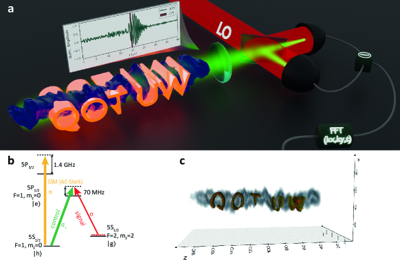
Figure 1: Experimental setup for 3D phase-sensitive atomic coherence imaging. a The light emitted from the atomic cloud that stores a phase modulated (QOT UW inscription) atomic coherence is detected in far field of the ensemble using a spatially-resolved heterodyne detector. The temporal shape of the emitted signal contains information associated with the longitudinal coherence wavevector. b Light-atoms interface used to generate, modulate and retrieve the atomic coherence (spin wave). c Full 3D Fourier transform $\mathcal{F}_{(k_{x},k_{y},k_{z}=-\beta t)\to(x,y,z)}$ of the registered signal $\Omega_{s}(k_{x},k_{y},t)$ gives the spin wave phase-and-amplitude distribution in real space $\mathcal{S}(x,y,z)$.

The experimental setup is schematically depicted in Fig. 1a. The base of the experiment is a pencil-shaped ($10\times 0.3\times 0.3\ \mathrm{mm}^{3}$) cloud of ⁸⁷Rb atoms formed in a magneto-optical trap (MOT) placed in a constant magnetic field along $z$-axis: $\mathbf{B}=\hat{z}B_{0}$, with $B_{0}\approx 1\,\mathrm{G}$. After releasing from the trap, atoms are optically pumped to $|g\rangle=5S_{1/2},F=2,m_{F}=2$ for 15 $\mu$s using two simultaneously working pumps. The first is 795 $\mathrm{nm}$ non-polarized laser tuned to $5S_{1/2},F=1\rightarrow 5P_{1/2},F=2$ transition which is intended to emptying $5S_{1/2},F=1$ hyperfine sublevel of the ⁸⁷Rb ground state. The second is 780 $\mathrm{nm}$ $\sigma_{+}$ circularly polarized laser tuned to $5S_{1/2},F=2\rightarrow 5P_{3/2},F=2$ transition illuminating atoms along the cloud (this direction we call $z$ axis), which provides magnetic sublevel pumping within the $5S_{1/2},F=2$ manifold, ideally populating only the $|g\rangle$ state.

After pumping, a strong atomic coherence $\varrho_{hg}$ between $|g\rangle$ and $|h\rangle=5S_{1/2},F=1,m_{F}=0$ states is generated in a $\Lambda$ scheme with excited state $|e\rangle=5P_{1/2},F=2,m_{F}=1$, coupled with mutually coherent write-in signal (at $|g\rangle\rightarrow|e\rangle$ transition) and the coupling beams (at $|e\rangle\rightarrow|h\rangle$ transition), as shown in Fig. 1b.

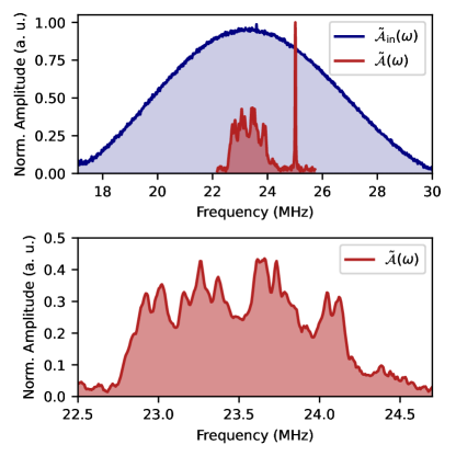
Figure 2: Panel a presents amplitude of 200 $\mathrm{ns}$ write-in pulse (blue) and read-out signal (red) measured with a heterodyne detection. The spectrum of the write-in signal is much wider than the bandwidth of the atomic cloud. The Zeeman splitting between the two-photon clock transition ($m_{F}=1\to m_{F}=-1$) and the memory transition ($m_{F}=2\to m_{F}=0$), caused by the magnetic field bias is also visible. Panel b presents the spectrum of the read-out signal from a.

To benchmark the tomography protocol we generate a flat atomic coherence across the whole atomic ensemble by writing in a very short $200\ \mathrm{ns}$ input signal pulse accompanied by coupling pulse of the same duration. Together they drive a two-photon transition between $|g\rangle$ excited state $|e\rangle=5P_{1/2},F=2,m_{F}=1$, and final state $|h\rangle=5S_{1/2},F=1,m_{F}=0$. Such a short pulse populates spin waves along the entire length of the cloud evenly, as the bandwidth of the write-in signal pulse is much larger than the magnetically (inhomogeneously) broadened two-photon absorption spectrum of the cloud. This was verified in measurement shown in Figure 2a where we compare the Fourier magnitude of heterodyne detected write-in and read-out signals. Here, we used a single point, differential photodiode (DPD) detector. The measurement yields bandwidths of about $8\,\mathrm{MHz}$ for the write-in signal and $\approx 1.4\,\mathrm{MHz}$ for the registered readout signal that directly corresponds to the GEM bandwidth induced by the Zeeman splitting gradient of around $1.4\,\mathrm{MHz/cm}$. Importantly, the Fourier magnitude of the input signal is flat across GEM spectrum which guarantees the creation of a flat spin-wave. Moreover, in the Figure 2b we show zoomed plot of the Fourier-magnitude of the readout signal that corresponds to the ($x$, $y$)-averaged atomic density along the $z$-axis.

For the full 3D reconstruction of $\mathcal{S}(x,y,z)$ we replace the DPD with an sCMOS camera located in the far field of the ensemble with an effective focal length of about 250mm. The two components of the heterodyne optical signal are registered on two separate regions of the camera that are then precisely aligned and subtracted to yield differential images. The camera has a very limited temporal resolution (exposure time of the order of 1 ms corresponds to 1 kHz bandwidth) which would mar the z-resolution. However, in GEM the temporal structure of the read-out signal can be probed using a very short coupling pulse. Therefore, full 3D spin-wave tomography is realized in a sequence of measurements. In a single step, the coupling is turned on for only $200\ \mathrm{ns}$, during which the probe read-out signal is generated and registered by the camera. For each probing time $t_{R}$ we collect 100 frames that are Fourier-filtered and coherently averaged in a real-time. The filtering and averaging strongly decrease the noise that is not correlated with the signal. The Fourier filtering step in this coherent detection process corresponds to only taking into account the signal which originated from the atoms and cutting the components that could not be created from within the cloud $x$-$y$ radius. Then to reconstruct entire $\mathcal{S}(x,y,z)$ we register signal for 600 distinct coupling pulse delays at a step of $100\ \mathrm{ns}$. Finally, we get a three-dimensional array, which is a full Fourier transform of the spin waves stored in the atomic ensemble.

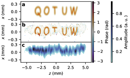
Figure 3: a “QOT UW” inscription phase imprinted onto atomic coherence between write-in and read-out b Phase of three-dimensional Fourier transform of the read-out signal with compensation of both diffraction and disappearing eddy current. c Amplitude of fully compensated three-dimensional Fourier transform of the read-out signal, which corresponds to atomic concentration. The right column corresponds to the simulation result.

To benchmark and calibrate our device we use ac-Stark spatial spin-wave phase modulator (SSM) [26]. Using spatial light modulator (SLM) and the camera we are able to prepare a beam with arbitrarily chosen intensity distribution, which illuminates atoms for 3 $\mu$s between the write-in and read-out. Thanks to the ac-Stark effect, atomic coherence gets an additional phase which is proportional to the intensity of illuminating light. A detailed description of spatial modulation of the spin-wave phase can be found in [26, 27, 28]. Figure 3 shows retrieved phase and amplitude profiles of a flat spin wave phase modulated with an inscription “QOT UW” (abbreviation of Quantum Optical Technologies, University of Warsaw). Figure 3a represents the displayed SSM pattern in phase (rad) units. In Fig. 3b we show the retrieved phase profile that well matches the target profile. Additionally, in Figure 3c we show retrieved spatial amplitude which in this case (flat spin wave) corresponds to the atomic concentration. The absolute phase value is obtained by subtracting the reference (ref) image that was acquired without the SSM modulation. The amplitude and the phase images are masked to display only the points that correspond to an atomic coherence magnitude much above the noise level $|\mathcal{S}^{\mathrm{ref}}(x,y,z)|>0.1$ and thus with a well-defined phase.

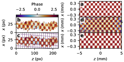
Figure 4: a Checkerboard phase profile imprinted onto atomic coherence between write-in and read-out we used for the calibration. b The phase of raw three-dimensional Fourier transform of the read-out signal. b Phase of three-dimensional Fourier transform of the read-out signal with compensation of both diffraction and disappearing eddy current. The right column corresponds to a numerical simulation of the results from the left column.

The correct 3D reconstruction of the spin wave phase and amplitude requires calibration of the heterodyne camera setup. Figure 4a presents a checkerboard intensity profile of the ac-Stark beam, which we use for calibration. Panel b shows the phase cross-section of the full Fourier transform of the signal registered by the camera (without any compensation). The checkerboard can be recognized, but the retrieved image is blurred. To sharpen it, two phenomena must be taken into account. The first one is diffraction which manifests as an additional quadratic phase in a Fourier domain that each slice attains during propagation. The phase is $(z-z_{0})(k_{x}^{2}+k_{y}^{2})/(2k_{0})$, where $k_{0}$ is the wave number of emitted signal and $k_{x,y}$ are transverse components of the wave vector. In real space, this results in the blurred retrieved distribution in ($x$, $y$) subspace. The second phenomenon is caused by a slow decrease in magnetic field gradient strength during the read-out. This effectively chirps the read-out signal. In other words, the signal gets an additional quadratic phase in the temporal domain, that results in a blur in $z$-direction. The temporal phase to be compensated is $\zeta t^{2}$ with $\zeta=-0.01\;\text{rad}\cdot\mu\text{s}^{-2}$. Panel c presents retrieved phase checkerboard pattern after both compensations. We finally see that the image is in focus and sharp. The parameters ($z_{0}$ and $\zeta$) for optimal phase profiles have been determined to obtain the best sharpness of the resulting images. Moreover, as the test pattern is prepared in true real space coordinates, the calibration procedure also yields the scaling factors and rotation for $x,y,z$ axes. For this measurement, we extended the measurement time window by collecting data for 1000 read-out pulse delays spanning a range of $100\,\mathrm{\mu s}$.

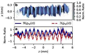
Figure 5: Slice of fully compensated three-dimensional Fourier transform of the read-out signal with two 200 ns pulses separated with 8 $\mu$s write-in signal. a Magnitude of two-dimensional $z$-$x$ slice of the normalized spin wave $\mathcal{S}(x,y,z)/\mathcal{S}^{\mathrm{ref}}(x,y,z)$. b Imaginary and real parts of the normalized coherence slice averaged over $x$-axis.

To demonstrate the ability to reconstruct an amplitude pattern of the spin wave we replace the flat spin wave with a modulated one. This is accomplished by using two short ($200\ \mathrm{ns}$) write in pulses ($200\ \mathrm{ns}$) separated by a delay of $\delta_{t}=8\ \mathrm{\mu s}$. The spectrum of two pulses of the same shapes yet different amplitudes, separated in time by $\delta t$ is a phase and amplitude modulated single pulse spectrum, given by the Fourier transform:

$$\mathcal{F}(\mathcal{A}(t)+\alpha\mathcal{A}(t+\delta_{t}))=\widetilde{\mathcal{A}}(\omega)(1+\alpha e^{i\omega\delta_{t}}).$$ (7)

Due to the spectrum to position mapping feature of GEM [29, 30] combined with the still meet the condition of large input signal bandwidth yields a spatially modulated coherence $\varrho_{hg}\propto(1+\alpha e^{2\pi i\delta_{t}\beta z})$. Figure 5a presents a two-dimensional magnitude slice $|\varrho_{hg}(x,z)|$ of the retrieved and fully compensated spin-wave pattern normalized to a flat spin wave corresponding to $\mathcal{A}(t)$: $\varrho_{hg}(x,y,z)=\mathcal{S}(x,y,z)/\mathcal{S}^{\mathrm{ref}}(x,y,z)$. The magnitude as expected resembles a squared cosine function $|\varrho_{hg}(x,z)|\propto\cos^{2}(2\pi\delta t\beta z)$ as the relative amplitude ratio is close to unity $\alpha\approx 1$. Panel b shows a decomposition of the normalized coherence slice $\varrho_{hg}(x,z)$ into imaginary and real parts averaged over the $x$-axis. The simultaneous phase and amplitude modulation are clearly visible.

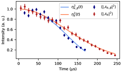
Figure 6: Thermal decoherence of the spin waves in GEM. Measured lifetimes are equal $\tau_{k}\approx 173\,\mathrm{\mu s}$ and $\tau_{\beta}\approx 175\,\mathrm{\mu s}$, which corresponds to $265\pm 15\,\mathrm{\mu K}$

The resolution in the perpendicular coordinates $(x,y)$ is limited by the optical imaging system, namely its numerical aperture. From the calibration images from Fig. 4 we can estimate the resolution as the half-width of the phase slope, which amounts to about 1 $\mathrm{px}$. That equals to $\delta x,\delta y\approx 14\,\mathrm{\mu m}$. The resolution along the propagation axis is however limited by the duration of the measurement window $T_{\mathrm{meas}}=100\,\mathrm{\{}\mu s\}$ combined with the magnitude of the magnetic field gradient $\beta=1.4\,\mathrm{MHz/cm}$. The longitudinal resolution could be then estimated by taking half of the inverse of the product of the measurement window and Zeeman splitting gradient: $\delta z\simeq 0.5/(T_{\mathrm{meas}}\beta)\approx 36\,\mathrm{\mu m}$. In the calibration images (Fig. 4c) we see that the width of the phase slope in the $z$-direction spans approximately 2 $\mathrm{px}$. This yields $44\,\mathrm{\mu m}$ of resolution. The maximal duration of the measurement window is in fact limited by the thermal motion of the atoms inside the ensemble. To estimate the rate of thermal decoherence caused by this motion we measured the read-out signal amplitude for range of read-out times $t_{\mathrm{R}}$. The results are presented in Figure 6. The measurements were performed, with and without magnetic field gradient. The thermal decoherence of spin waves in an atomic ensemble without the magnetic field gradient is well known and yields a Gaussian decay [31]. In the GEM the magnetic field gradient atoms travelling along the ensemble enter regions with different values of the magnetic field and attain additional phase. Namely, each group of atoms with velocity $v_{z}$ gains an additional phase factor of $\exp(i\beta v_{z}t_{\mathrm{R}}^{2}/4)$. That, after averaging with Maxwell velocity distribution gives additional exponential decoherence term with time in the fourth power. The full expression for the read-out decay reads:

$$\begin{gathered}\mathcal{\eta}_{k,\beta}(t)=e^{-\frac{t^{2}}{2\tau_{k}^{2}}-\frac{t^{4}}{2\tau_{\beta}^{4}}},\\ \tau_{k}=\frac{1}{k_{\mathrm{sw}}}\sqrt{\frac{m}{k_{b}T}}\text{, $\tau_{\beta}$=$\sqrt{\frac{2}{\pi\beta}\sqrt{\frac{m}{k_{b}T}}}$}\\ \\ \end{gathered}$$ (8)

where $k_{\text{sw}}$ is the spin-wave wavevector, $k_{b}$ is Boltzmann constant, $m$ is ⁸⁷Rb mass and $T$ is temperature of atomic cloud. The solid curves in Fig. 6 correspond to the above mode fitted to the experimental data. From the measurement without magnetic field gradient, we recover the characteristic time $\tau_{k}$ which in our case of the angle between the coupling and the write-in signal beam of $4.6\ \mathrm{mrad}$ equals $\tau_{k}=173\pm 5\,\mathrm{\mu s}$. The second measurement with the gradient turned on yields $\tau_{\beta}=175.4\pm 2.5\,\mathrm{\mu s}$. This corresponds to a temperature of $T=265\pm 15\,\mathrm{\mu K}$. To compensate for this decay in the reconstruction procedure we divide the measured signal $\mathcal{A}(t_{\mathrm{R}})$ by the factor $\eta_{k,\beta}(t_{\mathrm{R}})$.

Finally, we demonstrate the potential for application in 3D magnetometry by detecting a spin wave phase modulation caused by the magnetic field generated by a small coil placed near the atomic ensemble. The coil is turned on for a short period in the sequence between the write-in and read-out pulses. The inhomogeneous magnetic field generated by the coil imprints a phase that is proportional to the total magnitude of the magnetic field $|\mathbf{B}|$ and the interaction time $t_{c}$. The accumulated phase is $\varphi=\mu_{B}|\boldsymbol{\mathbf{B}}+\hat{z}B_{0}|t_{c}/\hbar$. The presence of the constant magnetic field along $z$-axis makes the phase sense mostly the changes of the field along the $z$-axis. However, one could easily imagine a more advanced protocol in which for the time of the measurement the constant field component is switched off. In such a scenario additionally to the phase modulation, one should observe amplitude modulation caused by the atomic spin rotation that yields different projections onto $z$-axis and modifies the readout efficiency (the coherence is partially transferred to a different magnetic sublevel, that is not coupled by the readout laser). Figure 7 shows the retrieved phase profile of the magnetically modulated coherence. The constant phase value lines correspond to the constant values of the local magnetic field.

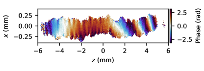
Figure 7: Retrieved phase of the coherence $\varrho_{hg}(x,z)$ affected by an inhomogeneous magnetic field generated by a small coil placed near the ensemble.

IV Conclusions

We have demonstrated how to reconstruct a 3D, the complex spatial distribution of atomic coherence $\varrho_{hg}(x,y,z)$. Or protocol relies on converting the coherence to be measured to light using a GEM protocol, heterodyne detection of readout pulse to recover its 3D phase and amplitude, unwinding phase due to diffraction and compensating for distortions which can be calibrated. The full 3D dependence of phase and amplitude of readout light can be recovered by repeating the experiment with short readout pulses, which play a role a time gating. This way we were able to complete our demonstration with a standard camera.

We have shown how to reconstruct a 3D, the complex spatial distribution of atomic coherence $\varrho_{hg}(x,y,z)$. Our method employs a magnetic field gradient to map the longitudinal components of the coherence onto read-out signal frequency. A single spatio-temporarlly resolved heterodyne measurement of the read-out light allows reconstruction of the full complex distribution of the atomic coherence $S(x,y,z)=n(x,y,z)\varrho_{h,g}(x,y,z)$. Here for the detection, we use a time-gated camera that requires many (short) measurements corresponding to different components on the reciprocal space of the propagation axis. However, a 2D array of photodiodes coupled with fast analog to digital converters would allow a single-shot measurement of the full 3D distribution. Moreover, a much simpler 1D array could be used in a hybrid measurement scheme with one of the axis resolved using a rainbow heterodyning technique [32] enabled by a multi-frequency LO with frequency gradient along the given (orthogonal to the array) axis. Finally, the demonstrated 3D magnetometry protocol could be extended to allow the 3D tomography of electric and electromagnetic fields in the microwave regime [33], opening a new kind of atom-based metrology. Beyond measuring external influences, the three-dimensional structure of Rydberg-atom interactions and propagation of Rydberg polaritons could be interrogated with the presented method, in order to generate unusual states of matter such as Efimov states [34] efficiently.