Global Convergence of SGD On Two Layer Neural Nets

Abstract

In this note, we demonstrate provable convergence of SGD to the global minima of appropriately regularized $\ell_{2}-$empirical risk of depth $2$ nets – for arbitrary data and with any number of gates, if they are using adequately smooth and bounded activations like sigmoid and tanh. We critically leverage having a constant amount of Frobenius norm regularization on the weights, along with a sampling of the initial weights from an appropriate class of distributions. We also prove an exponentially fast convergence rate for continuous time SGD that also applies to smooth unbounded activations like SoftPlus. Our key idea is to show the existence of loss functions on constant-sized neural nets which are “Villani functions” and thus be able to build on recent progress with analyzing SGD on such objectives.

1 Introduction

Modern developments in artificial intelligence have been significantly been driven by the rise of deep-learning - which in turn has been caused by the fortuitous coming together of three critical factors, (1) availability of large amounts of data (2) increasing access to computing power and (3) methodological progress. This work is about developing our understanding of some of the most ubiquitous methods of training nets. In particular, we shed light on how regularization can aid the analysis and help prove convergence to global minima for stochastic gradient methods for neural nets in hitherto unexplored and realistic parameter regimes.

In the last few years, there has been a surge in the literature on provable training of various kinds of neural nets in certain regimes of their widths or depths, or for very specifically structured data, like noisily realizable labels. Motivated by the abundance of experimental studies it has often been surmised that Stochastic Gradient Descent (SGD) on neural net losses – with proper initialization and learning rate – converges to a low–complexity solution, one that generalizes – when it exists Zhang et al. (2018). But, to the best of our knowledge a convergence result for any stochastic training algorithm for even depth $2$ nets (one layer of activations with any kind of non–linearity), without either an assumption on the width or the data, has remained elusive so far.

In this work, we not only take a step towards addressing the above question in the theory of neural networks but we also do so while keeping to a standard algorithm, the Stochastic Gradient Descent (SGD). In light of the above, our key message can be summarily stated as follows,

Theorem 1.1 (Informal Statement of the Main Result, Theorem 3.2).

If the initial weights are sampled from an appropriate class of distributions, then for nets with a single layer of sigmoid or tanh gats – for arbitrary data and size of the net – SGD on appropriately regularized $\ell_{2}-$losses, while using constant steps of size ${\mathcal{O}}(\epsilon)$, will converge in ${\mathcal{O}}(\frac{1}{\epsilon})$ steps to weights at which the expected regularized loss would be $\epsilon$–close to its global minimum.

We note that the threshold amount of regularization needed in the above would be shown to scale s.t it can either naturally turn out to be proportionately small if the norms of the training data are small or be made arbitrarily small by choosing outer layer weights to be small. Our above result is made possible by the crucial observation informally stated in the following lemma - which infact holds for more general nets than what is encompassed by the above theorem,

Lemma 1.2.

It is possible to add a constant amount of Frobenius norm regularization on the weights, to the standard $\ell_{2}-$loss on depth-$2$ nets with activations like SoftPlus, sigmoid and tanh gates s.t with no assumptions on the data or the size of the net, the regularized loss would be a Villani function.

Since our result stated above does not require any assumptions on the data, or the neural net width, we posit that this significantly improves on previous work in this direction. To the best of our knowledge, similar convergence guarantees in the existing literature require either some minimum neural net width – growing quickly w.r.t. inverse accuracy and the training set size (NTK regime Chizat et al. (2018); Du et al. (2018b)), infinite width (Mean Field regime Chizat & Bach (2018); Chizat (2022); Mei et al. (2018)) or other assumptions on the data when the width is parametric (e.g. realizable data, Ge et al. (2019); Zhou et al. (2021)). In contrast to all these, we show that with appropriate $\ell_{2}$ regularization, SGD on mean squared error (MSE) loss on 2–layer sigmoid / tanh nets converges to the global infimum. Our critical observation towards this proof is that the above loss on 2–layer nets – for a broad class of activation functions — is a “Villani function”. Our proof get completed by leveraging the relevant results in Shi et al. (2020).

Organization

In Section 2 we shall give a detailed review of the various approaches towards provable learning of neural nets. In Section 3 we present our theorem statements – our primary result being Theorem 3.2 which shows the global convergence of SGD and for gates like sigmoid and tanh. Additionally, in Theorem 3.4 we also point out that for our architecture if using the SoftPlus activation, we can show that the underlying SDE converges in expectation to the global minimizer in linear time. In Section 4, we give a brief overview of the methods in Shi et al. (2020), leading up to the proof of Theorem 3.2 in Section 5. In Section 6 we discuss some experimental demonstrations that our regularizer does not overshadow the original loss function. We end in Section 7 with a discussion of various open questions that our work motivates. In Appendix A one can find the calculations needed in the main theorem’s proofs.

2 Related Work

Review of the NTK Approach To Provable Neural Training :

One of the most popular parameter zones for theory has been the so–called “NTK” (Neural Tangent Kernel) regime – where the width is a high degree polynomial in the training set size and inverse accuracy (a somewhat unrealistic regime) and the net’s last layer weights are scaled inversely with width as the width goes to infinity, Lee et al. (2017); Wu et al. (2019); Du et al. (2018a); Su & Yang (2019); Kawaguchi & Huang (2019); Huang & Yau (2019); Allen-Zhu et al. (2019b; a; c); Du & Lee (2018); Zou et al. (2018); Zou & Gu (2019); Arora et al. (2019b; c); Li et al. (2019); Arora et al. (2019a); Chizat et al. (2018); Du et al. (2018b). The core insight in this line of work can be summarized as follows: for large enough width, SGD with certain initializations converges to a function that fits the data perfectly, with minimum norm in the RKHS defined by the neural tangent kernel – which gets specified entirely by the initialization (which is such that the initial output is of order one). A key feature of this regime is that the net’s matrices do not travel outside a constant radius ball around the starting point – a property that is often not true for realistic neural net training scenarios.

In particular, for the case of depth $2$ nets with similarly smooth gates as we focus on, in Song et al. (2021) global convergence of gradient descent was shown using number of gates scaling sub-quadratically in the number of data - which, to the best of our knowledge, is the smallest known width requirement for such a convergence in a regression setup. On the other hand, for the special case of training depth $2$ nets with $\mathop{\mathrm{ReLU}}$ gates on cross-entropy loss for doing binary classification, in Ji & Telgarsky (2020) it was shown that one needs to blow up the width only poly-logarithmically with target accuracy to get global convergence for SGD. In there it was pointed out as an important open question to determine whether one can get such reduction in width requirement for the regression setting too. The result we present here can be seen as an affirmative answer to this question posed in Ji & Telgarsky (2020).

Review of the Mean-Field Approach To Provable Neural Net Training :

In a separate direction of attempts towards provable training of neural nets, works like Chizat & Bach (2018) showed that a Wasserstein gradient flow limit of the dynamics of discrete time algorithms on shallow nets, converges to a global optimizer – if the convergence of the flow is assumed. We note that such an assumption is very non-trivial because the dynamics being analyzed in this setup is in infinite dimensions – a space of probability measures on the parameters of the net. Similar kind of non–asymptotic convergence results in this so–called ‘mean–field regime’ were also obtained in Mei et al. (2018; 2019); Fang et al. (2021); Chizat & Bach (2018); Chizat (2022); Tzen & Raginsky (2020); Jacot et al. (2018); Nguyen & Pham (2020); Sirignano & Spiliopoulos (2022; 2020b; 2020a); Ren & Wang (2022). In a recently obtained generalization of these insights to deep nets, Fang et al. (2021) showed convergence of the mean–field dynamics for ResNets He et al. (2016). The key idea in the mean–field regime is to replace the original problem of neural training which is a non-convex optimization problem in finite dimensions by a convex optimization problem in infinite dimensions – that of probability measures over the space of weights. The mean–field analysis necessarily require the probability measures (whose dynamics is being studied) to be absolutely–continuous and thus de facto it only applies to nets in the limit of them being infinitely wide.

We note that the results in the NTK regime hold without regularization while in many cases the mean–field results need it Mei et al. (2018); Chizat (2022); Tzen & Raginsky (2020).

In the next subsection we shall give a brief overview of some of the attempts that have been made to get provable deep-learning at parametric width.

Need And Attempts To Go Beyond Large Width Limits of Nets

The essential proximity of the NTK regime to kernel methods and it being less powerful than finite nets has been established from multiple points of view Allen-Zhu & Li (2019); Wei et al. (2019).

In He & Su (2020), the authors had given a a very visibly poignant way to see that the NTK limit is not an accurate representation of a lot of the usual deep-learning scenarios. Their idea was to define a notion of “local elasticity” – when doing a SGD update on the weights using a data say ${\bm{x}}$, it measures the fractional change in the value of the net at a point ${\bm{x}}^{\prime}$ as compared to ${\bm{x}}$. It’s easy to see that this is a constant function for linear regression - as is what happens at the NTK limit (Theorem 2.1 Lee et al. (2019)). But it has been shown in Dan et al. (2021) that this local-elasticity function indeed has non-trivial time-dynamics (particularly during the early stages of training) when a moderately large neural net is trained on a $\ell_{2}-$ loss.

In Liu et al. (2020) it was pointed out that the near-constancy of the tangent kernel might not happen for even very wide nets if there is an activation at the output layer – but still linear time gradient descent convergence can be shown. A set of attempts have also been made to bridge the gap between real-world nets and the NTK paradigm by adding terms which are quadratic in weights to the linear predictor that NTK considers, Zhu et al. (2022), Bai & Lee (2020), Hanin & Nica (2020)

On the other hand, recently in Hutzenthaler et al. (2021), asymptotic convergence of SGD has been proven for $\ell_{2}-$loss on arbitrary $\mathop{\mathrm{ReLU}}$ architectures – but for constant labels. Similar progress has also happened recently for G.D. in Chatterjee (2022) and Banerjee et al. (2022).

Specific to depth-2 nets – as we consider here – there is a stream of literature where analytical methods have been honed to this setup to get good convergence results without width restrictions - while making other structural assumptions about the data or the net. Janzamin et al. (2015) was one of the earliest breakthroughs in this direction and for the restricted setting of realizable labels they could provably get arbitrarily close to the global minima. For non-realizable labels they could achieve the same while assuming a large width but in all cases they needed access to the score function of the data distribution which is a computationally hard quantity to know. In a more recent development, Awasthi et al. (2021) have improved over the above to include $\mathop{\mathrm{ReLU}}$ gates while being restricted to the setup of realizable data and its marginal distribution being Gaussian.

One of the first proofs of gradient based algorithms doing neural training for depth$-2$ nets appeared in Zhong et al. (2017). In Ge et al. (2019) convergence was proven for training depth-$2$ $\mathop{\mathrm{ReLU}}$ nets for data being sampled from a symmetric distribution and the training labels being generated using a ‘ground truth’ neural net of the same architecture as being trained – the so-called “Teacher–Student” setup. For similar distributional setups, some of the current authors had in Karmakar et al. (2020) identified classes of depth–$2$ $\mathop{\mathrm{ReLU}}$ nets where they could prove linear-time convergence of training – and they also gave guarantees in the presence of a label poisoning attack. The authors in Zhou et al. (2021) consider another Teacher–Student setup of training depth $2$ nets with absolute value activations. In this work, authors can get convergence in poly$(d,\frac{1}{\epsilon})$ time, in a very restricted setup of assuming Gaussian data, initial loss being small enough, and the teacher neurons being norm bounded and ‘well–separated’ (in angle magnitude). Cheridito et al. (2022) get width independent convergence bounds for Gradient Descent (GD) with ReLU nets, however at the significant cost of having the restrictions of being only an asymptotic guarantee and assuming an affine target function and one–dimensional input data. While being restricted to the Gaussian data and the realizable setting for the labels, an intriguing result in Chen et al. (2021) showed that fully poly-time learning of arbitrary depth 2 ReLU nets is possible if one is in the “black-box query model”.

Related Work on Provable Training of Neural Networks Using Regularization

Using a regularizer is quite common in deep-learning practice and in recent times a number of works have appeared which have established some of these benefits rigorously. In particular, Wei et al. (2019) show that for a specific classification task (noisy–XOR) definable in any dimension $d$, no NTK based 2 layer neural net can succeed in learning the distribution with low generalization error in $o(d^{2})$ samples, while in $O(d)$ samples one can train the neural net using Frobenius/$\ell_{2}-$norm regularization. Nakkiran et al. (2021) show that for a specific optimal value of the $\ell_{2}$- regularizer the double descent phenomenon can be avoided for linear nets - and that similar tuning is possible even for real world nets.

In the seminal work Raginsky et al. (2017), it was pointed out that one can add a regularization to a gradient Lipschitz loss and make it satisfy the dissipativity condition so that Stochastic Gradient Langevin Dynamics (SGLD) provably converges to its global minima. But SGLD is seldom used in practice, and to the best of our knowledge it remains unclear if the observation in Raginsky et al. (2017) can be used to infer the same about SGD. Also it remains open if there exists neural net losses which satisfy all the assumptions needed in the above result. We note that the convergence time in Raginsky et al. (2017) for SGLD is $\mathcal{O}\left(\frac{1}{\epsilon^{5}}\right)$ using an $\mathcal{O}\left(\epsilon^{4}\right)$ learning rate, while in our Theorem 3.2 SGD converges in expectation to the global infimum of the regularized neural loss in time, $\mathcal{O}\left(\frac{1}{\epsilon}\right)$ using a $\mathcal{O}\left(\epsilon\right)$ step-length.

In summary, to the best of our knowledge, it has remained an unresolved challenge to show convergence of SGD on any neural architecture with a constant number of gates while neither constraining the labels nor the marginal distributional of the data to a specific functional form. In this work, for certain natural neural net losses, we are able to resolve this in our key result Theorem 3.2. Thus we take a step towards bridging this important lacuna in the existing theory of stochastic optimization for neural nets in general.

3 Setup and Main Results

We start with defining the neural net architecture, the loss function and the algorithm for which we prove our convergence result.

Definition 1 (Constant Step-Size SGD On Depth-2 Nets).

Let, $\sigma:\mathbb{R}\rightarrow\mathbb{R}$ (applied elementwise for vector valued inputs) be atleast once differentiable activation function. Corresponding to it, consider the width $p$, depth $2$ neural nets with fixed outer layer weights ${\bm{a}}\in\mathbb{R}^{p}$ and trainable weights $\mathbf{W}\in\mathbb{R}^{p\times d}$ as,

$$\mathbb{R}^{d}\ni{\bm{x}}\mapsto f({\bm{x}};\,{\bm{a}},\mathbf{W})={\bm{a}}^{\top}\sigma(\mathbf{W}{\bm{x}})\in\mathbb{R}$$

Then corresponding to a given set of $n$ training data $({\bm{x}}_{i},y_{i})\in\mathbb{R}^{d}\times\mathbb{R}$, with $\norm{{\bm{x}}_{i}}_{2}\leq B_{x},\absolutevalue{y_{i}}\leq B_{y},~{}i=1,\ldots,n$ define the individual data losses $\tilde{L}_{i}(\mathbf{W})\coloneqq\frac{1}{2}\left(y_{i}-f({\bm{x}}_{i},{\bm{a}};\mathbf{W})\right)^{2}$. Then for any $\lambda>0$ let the regularized empirical risk be,

$$\tilde{L}(\mathbf{W})\coloneqq\frac{1}{n}\sum_{i=1}^{n}\tilde{L}_{i}(\mathbf{W})+\frac{\lambda}{2}\norm{\mathbf{W}}_{F}^{2}$$ (1)

We implement on above the SGD with step-size $s>0$ as,

$$\mathbf{W}^{k+1}=\mathbf{W}^{k}-\frac{s}{b}\sum_{i\in\mathcal{B}_{k}}\nabla\tilde{L}_{i}(\mathbf{W}^{k})-s\lambda\mathbf{W}^{k}$$

where $\mathcal{B}_{k}$ is a randomly sampled mini-batch of size $b$.

Definition 2 (Properties of the Activation $\sigma$).

Let the $\sigma$ used in Definition 1 be bounded s.t. $\absolutevalue{\sigma(x)}\leq B_{\sigma}$, $C^{\infty}$, $L-$Lipschitz and $L_{\sigma}^{\prime}-$smooth. Further assume that $\exists$ a constant vector ${\bm{c}}$ and positive constants $B_{\sigma},M_{D}$ and $M_{D}^{\prime}$ s.t $\sigma(\mathbf{0})={\bm{c}}$ and $\forall x\in\mathbb{R},\absolutevalue{\sigma^{\prime}(x)}\leq M_{D},\absolutevalue{\sigma^{\prime\prime}(x)}\leq M_{D}^{\prime}$ .

In terms of the above constants we can now quantify the smoothness of the empirical loss as follows,

Lemma 3.1.

In the setup of Definition 1 and given the definition of $M_{D}$ and $L$ as above, there exists a constant $\lambda_{c}:=2\,M_{D}LB_{x}^{2}\norm{{\bm{a}}}_{2}^{2}$ s.t $\forall~{}\lambda>\lambda_{c}~{}\&~{}s>0$, the Gibbs’ measure $\sim\exp\left(-\frac{2\tilde{L}}{s}\right)$ satisfies a Poincaré-type inequality with the corresponding constant $\lambda_{s}$. Moreover, if the activation satisfies the conditions in Definition 2 then $\exists~{}{\rm gLip}(\tilde{L})>0$ s.t. the empirical loss, $\tilde{L}$ is ${\rm gLip}(\tilde{L})-$smooth and we can bound the smoothness coefficient of the empirical loss as,

$${\rm gLip}(\tilde{L})\leq\sqrt{p}\left({\norm{{\bm{a}}}_{2}B_{x}}B_{y}L_{\sigma}^{\prime}+\sqrt{p}\norm{{\bm{a}}}_{2}^{2}M_{D}^{2}B_{x}^{2}+{{p}\norm{{\bm{a}}}_{2}^{2}B_{x}^{2}}M_{D}^{\prime}B_{\sigma}+\lambda\right)$$

The precise form of the Poincaré-type inequality used above is detailed in Theorem 4.1.

Theorem 3.2 (Global Convergence of SGD on Sigmoid and Tanh Neural Nets of $2$ Layers for Any Width and Data).

We continue in the setup of Definitions 1, 2 and Lemma 3.1. For any $s>0$, define the probability measure $\mu_{s}\coloneqq\frac{1}{Z_{s}}\exp\left({-\frac{2\tilde{L}(\mathbf{W})}{s}}\right)$, $Z_{s}$ being the normalization factor. Then, $\forall~{}T>0,$ and desired accuracy, $\epsilon>0$, $\exists$ constants $A(\tilde{L})$, $B(T,\tilde{L})$ and $C(s,\tilde{L})$ s.t if the above SGD is executed at a constant step-size $s=s^{*}\coloneqq\min\left(\frac{1}{{\rm gLip}(\tilde{L})},\frac{\epsilon}{2\cdot(A(\tilde{L})+B(T,\tilde{L}))}\right)$ with the weights $\mathbf{W}^{0}$ initialized from a distribution with p.d.f $\rho_{\rm initial}\in L^{2}(\frac{1}{\mu_{s^{*}}})$ and $\norm{\rho_{\rm initial}-\mu_{s^{*}}}_{\mu_{s^{*}}^{-1}}\leq\frac{\epsilon}{2\cdot C(s^{*},\tilde{L})}\cdot e^{\lambda_{s^{*}}\cdot T}$ – then, in expectation, the regularized empirical risk of the net, $\tilde{L}$ would converge to its global infimum, with the rate of convergence given as,

$${\mathbb{E}}\tilde{L}(\mathbf{W}^{\frac{T}{s^{*}}})-\inf_{\mathbf{W}}\tilde{L}(\mathbf{W})\leq\epsilon.$$

The proof of the above theorem is given in Section 5 and the proof of Lemma 3.1 can be read off from the calculations done as a part of the proof of Theorem 3.2.

We make a few quick remarks about the nature of the above guarantee,

Firstly, we note that the “time horizon” $T$ above is a free parameter - which in turn parameterizes the choice of the step-size and the initial weight distribution. Choosing a larger $T$ makes the constraints on the initial weight distribution weaker at the cost of making the step-size smaller and the required number of SGD steps larger. But for any value of $T$, the above theorem guarantees that SGD, initialized from weights sampled from a certain class of distributions, converges in expectation to the global minima of the regularized empirical loss for our nets for any data and width, in time ${\mathcal{O}}(\frac{1}{\epsilon})$ using a learning rate of ${\mathcal{O}}(\epsilon)$.

Secondly, we note that the phenomenon of a lower bound on the regularization parameter being needed for certain nice learning theoretic property to emerge has been seen in kernel settings too, Yang et al. (2017).

Also, to put into context the emergence of a critical value of the regularizer for nets as in the above theorem, we recall the standard result, that there exists an optimal value of the $\ell_{2}-$regularizer at which the excess risk of the similarly penalized linear regression becomes dimension free (Proposition 3.8, Bach (2022)). However, we recall that the quantities required for computing this “optimal” regularizer are not knowable while training and hence it is not practically implementable. Thus, we see that for linear regression one can define a notion of an “optimal” regularizer and it remains open to investigate if such a similar threshold of regularization also exists for nets. Our above theorem can be seen as a step in that direction.

Thirdly, we note that the lowerbounds on training time of neural nets proven in works like Goel et al. (2020) do not apply here since these are proven for SQ algorithms and SGD is not of this type.

Finally, note that the threshold value of regularization computed above, $\lambda_{c}$, does not explicitly depend on the training data or the neural architecture, consistent with observations in Anthony & Bartlett (2009); Zhang et al. (2021). It depends on the activation and scales with the norm of the input data and the outer layer of weights. For intuition, suppose we scale the outer layer weights s.t we always have $\norm{{\bm{a}}}_{2}\cdot B_{x}=1$. Then this leads to $\lambda_{c}=2\cdot M_{D}L.$ For the sigmoid activation, $\sigma_{\beta}(x)=\frac{1}{1+e^{-\beta x}}.$ we have, $M_{D}=L=\frac{\beta}{4}$ and hence the $\lambda_{c}$ in this case (say $\lambda_{c,\beta}^{si}$) is $=\frac{\beta^{2}}{8}.$ Since $\beta=1$ is the most widely used setting for the above sigmoid activation, we use the same for our experiments. This results in,

$$\lambda_{c,1}^{si}=0.125$$ (2)

In experiments (Section 6) we demonstrate that the degradation in performance due to the above regularization is not very significant.

3.1 Global Convergence of Continuous Time SGD on Nets with SoftPlus Gates

In, Shi et al. (2020) the authors had established that, if the loss $\tilde{L}$ is gradient Lipschitz, then over any fixed time horizon $T>0$, as $s\rightarrow 0$, the dynamics of the SGD in Definition 1 is arbitrarily well approximated (in expectation) by the unique global solution that exists for the Stochastic Differential Equation (SDE),

$$\differential{{\mathbf{W}}_{s}(t)}=-\nabla\tilde{L}(\mathbf{W}_{s}(t))\differential{t}+\sqrt{s}\differential{{\mathbf{B}}(t)}\quad\quad\text{(SGD--SDE)}$$ (3)

where ${\mathbf{B}}(t)$ is the standard Brownian motion. The SGD convergence proven in the last section critically uses this mapping to a SDE. In Shi et al. (2020) it was further pointed out that if we only want to get a non-asymptotic convergence rate for the continuous time dynamics, the smoothness of the loss function is not needed and only the Villani condition suffices. In this short section we shall exploit this to show convergence of continuous time SGD on $\tilde{L}$ with the activation function being the unbounded ‘SoftPlus’. Also, in contrast to the guarantee about SGD in the previous subsection here we shall see that the SDE converges exponentially faster i.e at a linear rate.

Definition 3 (SoftPlus activation).

For $\beta>0,$ $x\in\mathbb{R},$ define the SoftPlus activation function as

$${\rm SoftPlus}_{\beta}(x)=\frac{1}{\beta}\log_{e}{\left(1+\exp(\beta x)\right)}$$

Remark.

Note that $\lim_{\beta\rightarrow\infty}{\rm SoftPlus}_{\beta}(x)={\rm ReLU}(x).$ Also note that for $f(x)=$ SoftPlus${}_{\beta}(x)$, $f^{\prime}(x)=\sigma_{\beta}(x)$ (sigmoid function as defined above) and hence $\absolutevalue{f^{\prime}(x)}\leq M_{D}$ for $M_{D}=1$ and $f(x)$ is $L-$Lipschitz for $L=1$.

Recall the following fact that was proven as a part of Lemma 3.1,

Lemma 3.3.

There exists a constant $\lambda_{c}:=2\,M_{D}LB_{x}^{2}\norm{{\bm{a}}}_{2}^{2}$ s.t $\forall~{}\lambda>\lambda_{c}~{}\&~{}s>0$, the Gibbs’ measure $\mu_{s}\coloneqq\frac{1}{Z_{s}}\exp\left({-\frac{2\tilde{L}(\mathbf{W})}{s}}\right)$, $Z_{s}$ being the normalization factor, satisfies a Poincaré-type inequality with the corresponding constant $\lambda_{s}$.

Given all the definitions above, now we can state the key result we have about Soft-Plus nets,

Theorem 3.4 (Continuous Time SGD Converges to Global Minima of SoftPlus Nets in Linear Time).

We consider the SDE as given in Equation 4 on a Frobenius norm regularized $\ell_{2}$-empirical loss on depth$-2$ neural nets as specified in Equation 1, while using $\sigma(x)={\rm SoftPlus}_{\beta}(x)$ for $\beta>0$, the regularization threshold being s.t $\lambda>\lambda_{c}=2\,M_{D}LB_{x}^{2}\norm{{\bm{a}}}_{2}^{2}$ and with the weights $\mathbf{W}_{0}$ being initialized from a distribution with p.d.f $\rho_{\rm initial}\in L^{2}(\frac{1}{\mu_{s}})$.

Then, for any $S>0$, $\exists~{}G(S,\tilde{L})$ and $C(s,\tilde{L})$, an increasing function of $s$, s.t for any step size $0<s\leq\min\left\{\frac{\epsilon}{2G(S,\tilde{L})},S\right\}$ and for $t\geq\frac{1}{\lambda_{s}}\log{\left(\frac{2\,C(s,\tilde{L})\norm{\rho_{\rm initial}-\mu_{s}}_{\mu_{s}^{-1}}}{\epsilon}\right)}$ we have that,

$$\mathbb{E}\,\tilde{L}(\mathbf{W}(t))-\min_{\mathbf{W}}\tilde{L}(\mathbf{W})\leq\epsilon.$$

Proof.

The SoftPlus function is Lipschitz, hence using the same analysis as in (Appendix A), we can claim that for $\lambda>\lambda_{c}$ the loss function in Definition 1 with SoftPlus activations is a Villani function (and hence confining, by definition).

Then, from Proposition $3.1$ of Shi et al. (2020) it follows that, $\exists~{}C(s,\tilde{L})$, an increasing function of $s$, that satisfies,

$$\absolutevalue{\mathbb{E}\tilde{L}(\mathbf{W}_{s}(t))-\mathbb{E}\tilde{L}(\mathbf{W}_{s}(\infty))}\leq C(s,\tilde{L})\norm{\rho_{\rm initial}-\mu_{s}}_{\mu_{s}^{-1}}\,e^{-\lambda_{s}t}.$$

From Proposition $3.2$ of Shi et al. (2020) it follows that, for any $S>0$, for $s\in(0,S)$, $\exists~{}G(S,\tilde{L})$ that quantifies the excess risk at the stationary point of the SDE as,

$$\tilde{L}(\mathbf{W}(\infty))-\min_{\mathbf{W}}\tilde{L}\leq G(S,\tilde{L})\,s$$

Combining the above, the final result claimed follows as in Corollary $3.3$ in Shi et al. (2020). ∎

3.2 An Experimental Study of the Effect of Regularization at Various Widths

For further understanding of the scope of the known theory, in here we present some experimental studies on depth $2$ nets with sigmoid gates and using the normalizations that correspond to the theoretically needed threshold value of the regularizer being $0.125$ (equation 2). We simulate SGD based training of multiple neural nets (details about the data and other hyperparameters are given below the respective plots), across a range of $\lambda$ and neural net widths $p.$ As evident in the plot (Figs. 1, 2), the test loss values in our regularization regime ($\lambda>0.125$) are comparatively only mildly deteriorating, compared to regularizers upto four orders of magnitude lower. To the best of our knowledge, a similar provable convergence guarantee is not known for $\lambda<0.125,$ and hence the slightly larger test loss that we incur is only a minor trade-off.

Code for these experiments can be viewed in this Colab Notebook (link)

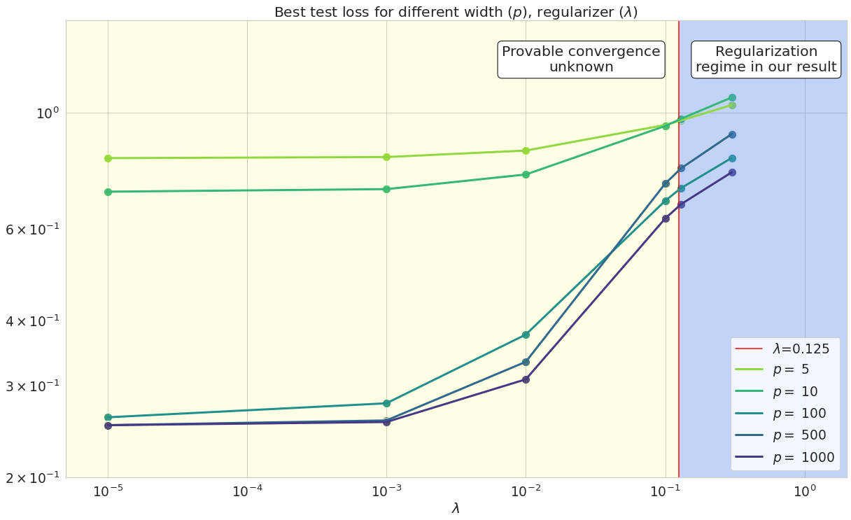
Figure 1: Best test loss across a range of $(\lambda,p={\rm width})$ for $({\mathbf{x}},y)$ data labeled as,

${\mathbf{x}}\sim{\rm Uniform}\left([0,1)^{20}\right),y=\sin\left(\pi\frac{\norm{{\mathbf{x}}}_{2}^{2}}{20}\right)+\epsilon;\,\epsilon\sim\mathcal{N}(0,0.25)$

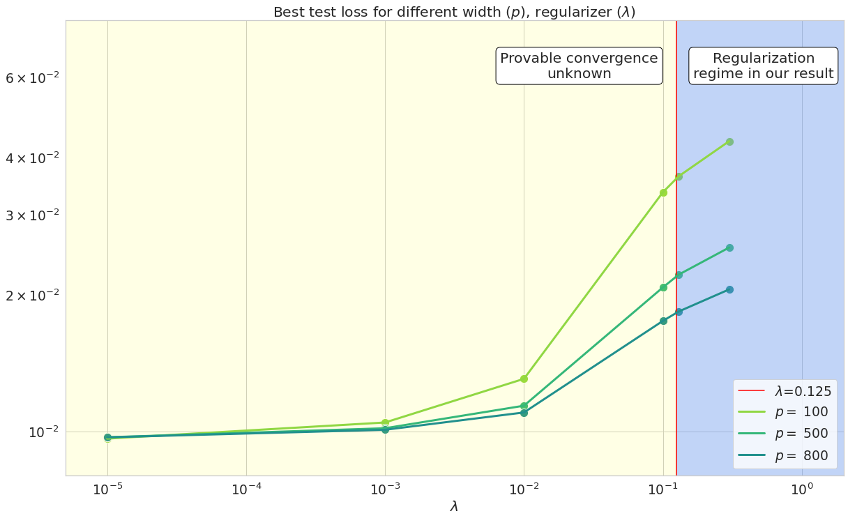
Figure 2: Best test loss across a range of $(\lambda,{\rm width}=p)$ for realizable data $({\mathbf{x}},y)$ sampled as,

${\mathbf{x}}\sim{\rm Uniform}\left([0,1)^{20}\right),y=\mathbf{a}^{\top}\sigma(\mathbf{W}\mathbf{{\mathbf{x}}})+\epsilon;\,p=5,\epsilon\sim\mathcal{N}(0,0.01),a_{i}\sim\frac{1}{\sqrt{p}}\mathcal{N}(0,1)$

4 Overview of Shi et al. (2020)

In Section 5, we give the proof for our main result (Theorem 3.2). As relevant background for the proof, we shall give in here a brief overview of the framework in Shi et al. (2020), which can be summarized as follows : suppose one wants to minimize the function $\tilde{L}(\mathbf{W})\coloneqq\frac{1}{n}\sum_{i=1}^{n}\tilde{L}_{i}(\mathbf{W})$, where $i$ indexes the training data, $\mathbf{W}$ is the parameter space (the optimization space) of the loss function and $\tilde{L}_{i}$ is the loss evaluated on the $i^{th}-$datapoint. On this objective, a constant step-size mini-batch implementation of the Stochastic Gradient Descent (SGD) consists of doing the following iterates, $\mathbf{W}_{k+1}=\mathbf{W}_{k}-\frac{s}{b}\sum_{i}\nabla\tilde{L}_{i}(\mathbf{W}_{k})$, where the sum is over a mini-batch (a randomly sampled subset of the training data) of size $b$ and $s$ is the fixed step-length. In, Shi et al. (2020) the authors established that over any fixed time horizon $T>0$, as $s\rightarrow 0$, the dynamics of this SGD is arbitrarily well approximated (in expectation) by the Stochastic Differential Equation (SDE),

$$\differential{\mathbf{W}_{s}(t)}=-\nabla\tilde{L}(\mathbf{W}_{s}(t))\differential{t}+\sqrt{s}\differential{\mathbf{B}(t)}\quad\quad\text{(SGD--SDE)}$$ (4)

where $\mathbf{B}(t)$ is the standard Brownian motion. We recall that the Markov semigroup operator $P_{t}$ for a stochastic process $X_{t}$ and its infinitesimal generator $\mathcal{L}$ are given as, $P_{t}f(x)\coloneqq\mathbb{E}[f(X_{t})\mid X_{0}=x]$ and $\mathcal{L}f\coloneqq\lim_{t\,\downarrow\,0}\,\frac{P_{t}f-f}{t}$. Thus for the SDE in Eq. 4, $\mathcal{L}$ and its adjoint $\mathcal{L}^{*}$ are given as

$$\mathcal{L}f=\frac{s}{2}\Delta f-\left\langle\nabla f,\nabla\tilde{L}\right\rangle\implies\mathcal{L^{*}}f=\left\langle\nabla{f},\nabla\tilde{L}\right\rangle+f\,\Delta\,\tilde{L}+\frac{s}{2}\Delta f$$

Then invoking the Forward Kolmogorov equation ${\partial_{t}f}=\mathcal{L}^{*}f$, one obtains the following Fokker–Planck–Smoluchowski PDE governing the evolution of the density of the SDE,

$$\partialderivative{\rho_{s}}{t} =\langle\nabla\rho_{s},\nabla\tilde{L}\rangle+\rho_{s}\Delta\tilde{L}+\frac{s}{2}\Delta\rho_{s}\quad\quad\text{(FPS)}$$ (5)

Further, under appropriate conditions on $\tilde{L}$ the above implies that the density $\rho_{s}(t)$ converges exponentially fast to the Gibbs’ measure corresponding to the objective function i.e the distribution with p.d.f

$$\mu_{s}=\frac{1}{Z_{s}}{\exp\left(-\frac{2\tilde{L}(\mathbf{W})}{s}\right)}$$

where $Z_{s}$ is the normalization factor. The sufficient conditions on $\tilde{L}$ that were shown to be needed to achieve this “mixing" and to know a rate for it, are that of $\tilde{L}$ being a “Villani Function” as defined below,

Definition 4 (Villani Function (Villani (2009); Shi et al. (2020))).

A map $f:\mathbb{R}^{d}\rightarrow\mathbb{R}$ is called a Villani function if it satisfies the following conditions,

1. $f\in C^{\infty}$

2. $\lim_{\norm{{\bm{x}}}\rightarrow\infty}f({\bm{x}})=+\infty$

3. ${\displaystyle\int_{\mathbb{R}^{d}}}\exp\left({-\frac{2f({\bm{x}})}{s}}\right)\differential{{\bm{x}}}<\infty~{}\forall s>0$

4. $\lim_{\norm{{\bm{x}}}\rightarrow\infty}\left(-\Delta f({\bm{x}})+\frac{1}{s}\cdot\norm{\nabla f({\bm{x}})}^{2}\right)=+\infty~{}\forall s>0$

Further, any $f$ that satisfies conditions 1 – 3 is said to be “confining”.

From Lemma $5.2$ Shi et al. (2020), the empirical or the population risk, $\tilde{L}$, being confining is sufficient for the FPS PDE (equation 5) to evolve the density of SGD–SDE (equation 4) to the said Gibbs’ measure.

But, to get non-asymptotic guarantees of convergence (Corollary $3.3$, Shi et al. (2020)) – even for the SDE, we need a Poincaré–type inequality to be satisfied (as defined below) by the aforementioned Gibbs’ measure $\mu_{s}$. A sufficient condition for this Poincaré–type inequality to be satisfied is if a confining loss function $\tilde{L}$ also satisfied the last condition in definition 4 (and is consequently a Villani function).

Theorem 4.1 (Poincaré–type Inequality (Shi et al. (2020))).

Given a $f:\mathbb{R}^{d}\rightarrow\mathbb{R}$ which is a Villani Function (Definition 4), for any given $s>0$, define a measure with the density, $\mu_{s}({\bm{x}})=\frac{1}{Z_{s}}{\exp\left(-\frac{2f({\bm{x}})}{s}\right)}$, where $Z_{s}$ is a normalization factor. Then this (normalized) Gibbs’ measure $\mu_{s}$ satisfies a Poincare-type inequality i.e $\exists~{}\lambda_{s}>0$ (determined by $f$) s.t $\forall h\in C_{c}^{\infty}(\mathbb{R}^{d})$ we have,

$${\rm Var}_{\mu_{s}}[h]\leq\frac{s}{2\lambda_{s}}\cdot\mathbb{E}_{\mu_{s}}[\norm{\nabla h}^{2}]$$

The approach of Shi et al. (2020) has certain key interesting differences from many other contemporary uses of SDEs to prove the convergence of discrete time stochastic algorithms. Instead of focusing on the convergence of parameter iterates $\mathbf{W}^{k}$, they instead look at the dynamics of the expected error i.e $\mathbb{E}[\tilde{L}(\mathbf{W}^{k})]$, for $\tilde{L}$ the empirical or the population risk. This leads to a transparent argument for the convergence of $\mathbb{E}[\tilde{L}(\mathbf{W}^{k})]$ to $\inf_{\mathbf{W}}\tilde{L}(\mathbf{W})$, by leveraging standard results which help one pass from convergence guarantees on the SDE to a convergence of the SGD.

We note that Shi et al. (2020) achieve this conversion of guarantees from SDE to SGD by additionally assuming gradient smoothness of $\tilde{L}$ – and we would show that this assumption holds for the natural neural net loss functions that we consider.

5 Proof of Theorem 3.2

Proof.

Note that $\tilde{L}$ being a confining function can be easily read off from Definition 4. Further, as shown in Appendix A, the following inequalities hold,

$$\norm{\nabla_{\mathbf{W}}\tilde{L}}_{2}^{2} \geq(\lambda^{2}-2\lambda M_{D}LB_{x}^{2}\norm{{\bm{a}}}_{2}^{2})\norm{\mathbf{W}}_{F}^{2}$$

$$-{2\lambda mM_{D}B_{x}\norm{{\bm{a}}}_{2}(B_{y}+\norm{{\bm{a}}}_{2}\norm{{\bm{c}}}_{2})\norm{\mathbf{W}}_{F}}$$ (6)

$$\Delta_{\mathbf{W}\mathbf{W}}\tilde{L} \leq p\left[M_{d}^{2}B_{x}^{2}\norm{{\bm{a}}}_{2}^{2}+{\norm{{\bm{a}}}_{2}}\left[\left(B_{y}+\norm{{\bm{a}}}_{2}\left(\norm{{\bm{c}}}_{2}+LB_{x}\norm{\mathbf{W}}_{F}\right)\right)\left(M_{D}^{\prime}B_{x}^{2}\right)\right]+\lambda d\right]$$ (7)

Combining the above two inequalities we can conclude that, $\exists$ functions $g_{1},g_{2},g_{3}$ such that,

$$\frac{1}{s}\norm{\nabla_{\mathbf{W}}\tilde{L}}^{2}-\Delta_{\mathbf{W}\mathbf{W}}\tilde{L} \geq g_{1}(\lambda,s)\norm{\mathbf{W}}_{F}^{2}-g_{2}(\lambda,s)\norm{\mathbf{W}}_{F}+g_{3}(\lambda,s)$$

where in particular,

$$g_{1}(\lambda,s)=\lambda^{2}-2\lambda\cdot M_{D}LB_{x}^{2}\norm{{\bm{a}}}_{2}^{2}.$$

Hence we can conclude that for $\lambda>\lambda_{c}\coloneqq 2M_{D}LB_{x}^{2}\norm{{\bm{a}}}_{2}^{2},\forall s>0,$ $\frac{1}{s}\norm{\nabla_{\mathbf{W}}\tilde{L}}^{2}-\Delta_{\mathbf{W}\mathbf{W}}\tilde{L}$ diverges as $\norm{\mathbf{W}}\rightarrow+\infty$, since $g_{1}(\lambda,s)>0.$ The key aspect of the above analysis being that the bound on $\Delta_{\mathbf{W}\mathbf{W}}$ does not depend on $\norm{\mathbf{W}}_{F}^{2}.$

Thus we have, that the following limit holds,

$$\lim_{\norm{\mathbf{W}}_{F}\rightarrow+\infty}\left(\frac{1}{s}\norm{\nabla_{\mathbf{W}}\tilde{L}}^{2}-\Delta_{\mathbf{W}\mathbf{W}}\tilde{L}\right)=+\infty$$

for the range of $\lambda$ as given in the theorem, hence proving that $\tilde{L}$ is a Villani function.

Towards getting an estimate of the step-length as given in the theorem statement, we also show in Appendix B that the loss function $\tilde{L}$ is gradient–Lipschitz with the smoothness coefficient being upperbounded as,

$${\rm gLip}(\tilde{L})\leq\sqrt{p}\left({\norm{{\bm{a}}}_{2}B_{x}}B_{y}L_{\sigma}^{\prime}+\sqrt{p}\norm{{\bm{a}}}_{2}^{2}M_{D}^{2}B_{x}^{2}+{{p}\norm{{\bm{a}}}_{2}^{2}B_{x}^{2}}M_{D}^{\prime}B_{\sigma}+\lambda\right).$$

Now we can invoke Theorem $3$ (Part 1), Shi et al. (2020) with appropriate choices of $s$ and initialization to get the main result as given in Theorem 3.2. In Appendix C one can find a discussion of the computation of the specific constants involved in the expression for the suggested step-length $s^{*}$ and the class of initial weight distribution p.d.fs $\rho_{\rm initial}$. ∎

6 Ablation Study with Noisy Labels

In this section, we give some further experimental studies of doing regression over nets that are within the ambit of our core result of Theorem 3.2. The demonstrations in this section are designed to address two conceptual issues,

1. Firstly, we verify that when using sigmoid gates and $\lambda$ slightly larger than the theoretically computed threshold of, $\lambda_{c,1}^{si}=0.125$ (Equation 2) it does not lead to the regularizer term in the loss overpowering the actual (empirical risk) objective. We demonstrate this by adding random noise (details follow) to the training labels and observing that the training / test loss values reached by the SGD degrades in response to increasing the fraction of noisy labels even at $\lambda=0.13>\lambda_{c,1}^{si}$.

2. Secondly, we verify that even when the neural net is not initialized from $\rho_{initial}$ as described in Theorem 3.2, the SGD converges and is affected by $\lambda$ tuning as would be expected from the theorem.

We train the neural net on 3 different synthetic training datasets: a) the clean version (generated as ${\bm{x}}\sim{U}[0,1)^{d},\,y=\sin{\left(\pi\frac{\norm{{\bm{x}}}_{2}^{2}}{d}\right)}$ and when b) $50\%$ and c) $90\%$ of the labels in the clean data have been additively corrupted by $0.05\cdot\xi,\,\xi\sim\text{Cauchy}(0,1).$

Recalling the theoretically computed threshold of, $\lambda_{c,1}^{si}=0.125$ (Equation 2) we choose $\lambda=0.013,0.13$ as two values above and below the threshold. We set $\norm{{\bm{a}}}_{2}=\frac{1}{B_{x}}$, $d=20$ (the data dimension). Further, we choose data such that $B_{x}=\sqrt{d}$, and choose 2 values for the number of gates $p$ – one which is half the data-dimension ($10$) and one which is more than double of it ($50$). Finally, the values of $p$, step-size $\eta$, and $\lambda$ are specified for each of the plots (in caption) in Figs. 3, 4, 5, 6.

In all experiments we see that the test loss on clean data (the middle figures in the panels below) progressively degrades with increasing the fraction of noisy labels in the training data – thus confirming that using $\lambda=0.13>\lambda_{c,1}^{si}$ regularization did not obfuscate the algorithm’s response to meaningful details of the unregularized loss.

Code for these experiments can be found at the following link: Colab notebook.

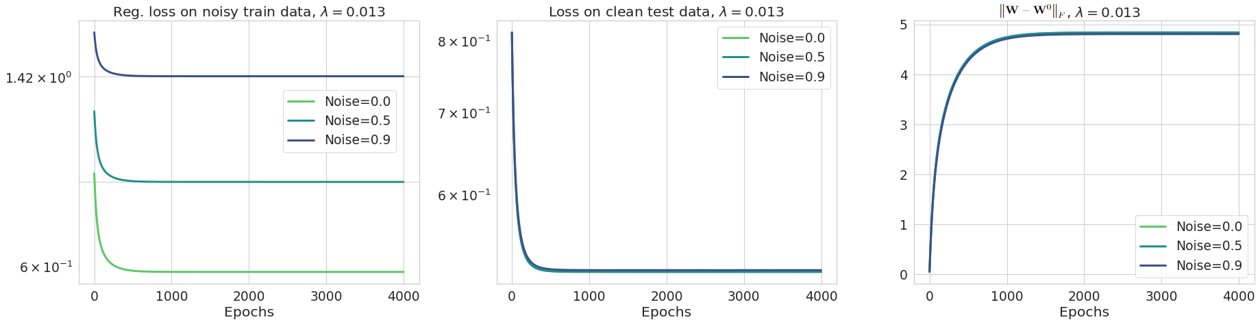
Figure 3: Regression, $(p,\eta,\lambda)=(10,1\text{e-}2,0.013)$

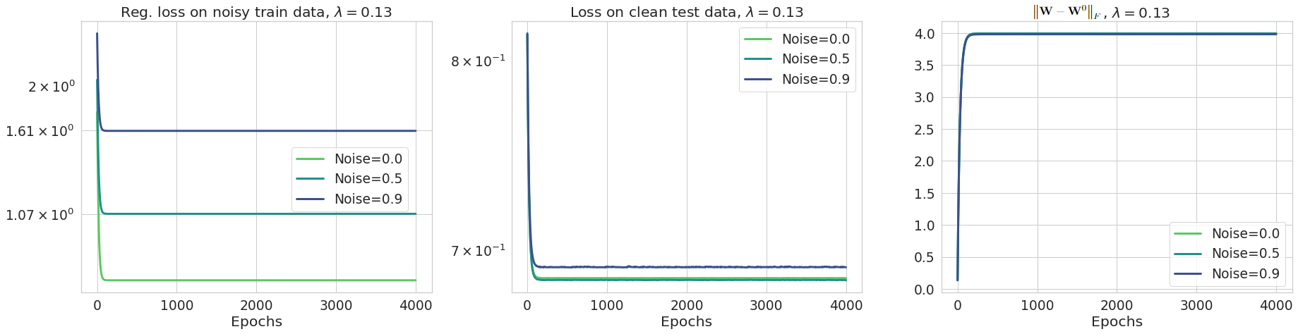
Figure 4: Regression, $(p,\eta,\lambda)=(10,1\text{e-}2,0.13)$

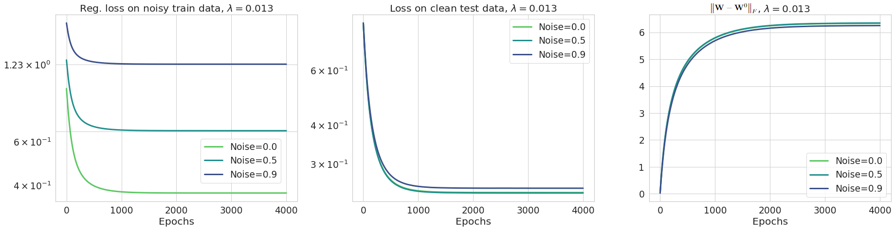
Figure 5: Regression, $(p,\eta,\lambda)=(50,5\text{e-}3,0.013)$

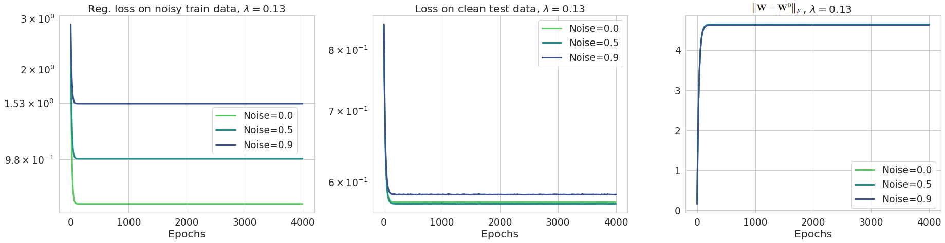
Figure 6: Regression, $(p,\eta,\lambda)=(50,1\text{e-}2,0.13)$

7 Conclusion

Convergence of discrete time algorithms like SGD to their continuous time counterpart (SDEs) has lately been an active field of research. Availability of a well–developed mathematical theory for SDEs holds potential for this mapping to makes theoretical analyses of stochastic gradient–based algorithms possible in hitherto unexplored regimes if the discrete time algorithm has a corresponding SDE to which its proximity is quantifiable.

In a recent notable progress in Li et al. (2021), an iterative algorithm called SVAG (Stochastic Variance Amplified Gradient) was introduced as a quantifiably good discretization of another SGD motivated SDE than what we use here. They show that SVAG iterates converge in expectation to the covariance–scaled Itô SDE. And they gave empirical evidence that this discretization and their SDE are also tracking SGD on real nets. It remains to be explored in future if this can become a pathway towards better guarantees on neural training than what we get here.

Additionally, we note that since SoftPlus is not bounded, using our current technique it does not follow that the SGD algorithm also converges to the global minimizer of its Frobenius norm regularized loss. Investigating the possibility of this result could be an exciting direction of future work. In general we believe that trying to reproduce our Theorem 3.2 using a direct analysis of the dynamics of SGD could be a fruitful venture leading to interesting insights. Lastly, our result motivates a new direction of pursuit in deep-learning theory, centered around understanding the nature of the Poincaré constant of Gibbs’ measures induced by neural nets.

Acknowledgments

We would like to thank Hadi Daneshmand and Zhanxing Zhu for their critical suggestions with setting up the experiments. Our work was hugely helped by Hadi sharing with us some of his existing code probing similar phenomenon as explored in our Section 6. We thank Matthew Colbrook and Siva Theja Maguluri for extensive discussions throughout this project. We are also grateful to Weijie Su, Siddhartha Mishra, Avishek Ghosh, Theodore Papamarkou, Alireza and Purushottam Kar for insightful comments at various stages of preparing this draft. In particular, we thank Daniel Soudry for his thoughtful queries about our work.

Appendix A Towards Establishing the Villani condition for the Empirical Loss on Nets

In the following, $\norm{\mathbf{W}}$ for a matrix $\mathbf{W}$ denotes its spectral or operator norm. We recall that the regularized $\ell_{2}-$loss for training the given neural net on data $\mathcal{D}=\{({\bm{x}}_{i},y_{i})\}_{i=1}^{n}$ is,

$$\tilde{L}(\mathbf{W})\coloneqq\frac{1}{n}\sum_{i=1}^{n}\tilde{L}_{i}(\mathbf{W})+R_{\lambda}({\mathbf{W}})\coloneqq\frac{1}{n}\sum_{i=1}^{n}\left\{\frac{1}{2}\left(y_{i}-f({\bm{x}}_{i};{\bm{a}},\mathbf{W})\right)^{2}\right\}+\frac{\lambda}{2}\norm{\mathbf{W}}_{F}^{2}$$

Explicitly stated, the SGD iterates with step-length $s>0$ that we analyze on the above loss are,

$$\mathbf{W}^{k+1} =\mathbf{W}^{k}-s\left[\frac{1}{b}\sum_{i\in\mathcal{B}_{k}}\nabla\tilde{L}_{i}(\mathbf{W}^{k})+\nabla R_{\lambda}({\mathbf{W}^{k}})\right]$$

$$=\mathbf{W}^{k}-\frac{s}{b}\sum_{i\in\mathcal{B}_{k}}\Big{(}-\left(y_{i}-f({\bm{x}}_{i};{\bm{a}},\mathbf{W}^{k})\right)\cdot\nabla_{\mathbf{W}^{k}}f({\bm{x}}_{i};{\bm{a}},\mathbf{W}^{k})\Big{)}-s\lambda\mathbf{W}^{k}$$

$$=(1-s\lambda)\mathbf{W}^{k}+\frac{s}{b}\sum_{i\in\mathcal{B}_{k}}\left[(y_{i}-f({\bm{x}}_{i};{\bm{a}},\mathbf{W}^{k}))\cdot\nabla_{\mathbf{W}^{k}}f({\bm{x}}_{i};{\bm{a}},\mathbf{W}^{k})\right]$$

We consider gradients and Laplacians of $\tilde{L}(\mathbf{W})$ w.r.t. $\mathbf{W}_{j},j=1,2,\ldots,p$ separately,

$$\nabla_{\mathbf{W}_{j}}\tilde{L} =\left[\frac{1}{n}\sum_{i=1}^{n}\left(f({\bm{x}}_{i};\,{\bm{a}},\mathbf{W})-y_{i}\right)\nabla_{\mathbf{W}_{j}}f({\bm{x}}_{i};\,{\bm{a}},\mathbf{W})\right]+\lambda\mathbf{W}_{j}$$

$$=\left[\frac{1}{n}\sum_{i=1}^{n}a_{j}\left(f({\bm{x}}_{i};\,{\bm{a}},\mathbf{W})-y_{i}\right)\sigma^{\prime}(\mathbf{W}_{j}^{\top}{\bm{x}}_{i}){\bm{x}}_{i}\right]+\lambda\mathbf{W}_{j}\quad;\quad j=1,2,\ldots,p$$

$$\implies\norm{\nabla_{\mathbf{W}_{j}}\tilde{L}}_{2}^{2} =\norm{\frac{1}{n}\sum_{i=1}^{n}a_{j}\left(f({\bm{x}}_{i};\,{\bm{a}},\mathbf{W})-y_{i}\right)\sigma^{\prime}(\mathbf{W}_{j}^{\top}{\bm{x}}_{i}){\bm{x}}_{i}}_{2}^{2}+\lambda^{2}\norm{\mathbf{W}_{j}}_{2}^{2}+$$

$$\quad\quad\quad\quad\quad\quad\quad\quad 2\left\langle\left[\frac{1}{n}\sum_{i=1}^{n}a_{j}\left(f({\bm{x}}_{i};\,{\bm{a}},\mathbf{W})-y_{i}\right)\sigma^{\prime}(\mathbf{W}_{j}^{\top}{\bm{x}}_{i}){\bm{x}}_{i}\right],\lambda\mathbf{W}_{j}\right\rangle$$

$$\geq\lambda^{2}\norm{\mathbf{W}_{j}}_{2}^{2}-\frac{2\lambda}{n}\left\langle\left[\sum_{i=1}^{n}a_{j}\left(y_{i}-f({\bm{x}}_{i};\,{\bm{a}},\mathbf{W})\right)\sigma^{\prime}(\mathbf{W}_{j}^{\top}{\bm{x}}_{i}){\bm{x}}_{i}\right],\mathbf{W}_{j}\right\rangle$$

$$\geq\lambda^{2}\norm{\mathbf{W}_{j}}_{2}^{2}-\frac{2\lambda\norm{\mathbf{W}_{j}}_{2}}{n}\left[\sum_{i=1}^{n}\absolutevalue{a_{j}}\cdot\left(\absolutevalue{y_{i}}+\norm{{\bm{a}}}_{2}\norm{\sigma(\mathbf{W}{\bm{x}}_{i})}_{2}\right)\cdot\absolutevalue{\sigma^{\prime}(\mathbf{W}_{j}^{\top}{\bm{x}}_{i})}\cdot\norm{{\bm{x}}_{i}}_{2}\right]$$

Where in the last inequality we have used Cauchy-Schwarz inequality and triangle inequality wherever applicable. We have,

$$\norm{\nabla_{\mathbf{W}_{j}}\tilde{L}}_{2}^{2} \geq\lambda^{2}\norm{\mathbf{W}_{j}}_{2}^{2}-\norm{\mathbf{W}_{j}}_{2}\absolutevalue{a_{j}}\cdot\Big{(}2\lambda M_{D}B_{x}\left\{B_{y}+\norm{{\bm{a}}}_{2}\cdot(LB_{x}\norm{\mathbf{W}}+\norm{{\bm{c}}}_{2})\right\}\Big{)}$$

In above we sum over $j=1,2,\ldots,p$ on both sides. Via Cauchy-Schwartz inequality we upperbound as, $\sum_{j=1}^{p}\norm{\mathbf{W}_{j}}_{2}\cdot\absolutevalue{a_{j}}\leq\norm{\mathbf{W}}_{F}\cdot\norm{{\bm{a}}}$ to get,

$$\norm{\nabla_{\mathbf{W}}\tilde{L}}^{2} \geq\lambda^{2}\norm{\mathbf{W}}_{F}^{2}-{\norm{{\bm{a}}}_{2}\norm{\mathbf{W}}_{F}}\cdot 2\lambda M_{D}B_{x}\cdot\left[B_{y}+(LB_{x}\norm{\mathbf{W}}+\norm{{\bm{c}}}_{2})\norm{{\bm{a}}}_{2}\right]$$

$$\geq\lambda^{2}\cdot\norm{\mathbf{W}}_{F}^{2}-2\lambda M_{D}LB_{x}^{2}\norm{{\bm{a}}}_{2}^{2}\cdot\norm{\mathbf{W}}_{F}\norm{\mathbf{W}}-{2\lambda M_{D}B_{x}\norm{{\bm{a}}}_{2}(B_{y}+\norm{{\bm{c}}}_{2}\cdot\norm{{\bm{a}}}_{2})\norm{\mathbf{W}}_{F}}$$

$$\geq\lambda^{2}\cdot\norm{\mathbf{W}}_{F}^{2}-2\lambda M_{D}LB_{x}^{2}\norm{{\bm{a}}}_{2}^{2}\cdot\norm{\mathbf{W}}_{F}^{2}-{2\lambda M_{D}B_{x}\norm{{\bm{a}}}_{2}(B_{y}+\norm{{\bm{c}}}_{2}\cdot\norm{{\bm{a}}}_{2})\norm{\mathbf{W}}_{F}}$$ (8)

In the last line above we used that, $\norm{\mathbf{W}}\leq\norm{\mathbf{W}}_{F}$.

Now, for $j=1,2,\ldots,p$ we have for the second derivatives,

$$\Delta_{\mathbf{W}_{j}\mathbf{W}_{j}}\tilde{L}=\nabla_{\mathbf{W}_{j}}\cdot\nabla_{\mathbf{W}_{j}}\tilde{L} =\nabla_{\mathbf{W}_{j}}\cdot\left[\left\{\frac{1}{n}\sum_{i=1}^{n}\left(f({\bm{x}}_{i};\,{\bm{a}},\mathbf{W})-y_{i})\right)\nabla_{\mathbf{W}_{j}}f({\bm{x}}_{i};\,{\bm{a}},\mathbf{W})\right\}+\lambda\mathbf{W}_{j}\right]$$

$$=\left[\frac{1}{n}\sum_{i=1}^{n}\nabla_{\mathbf{W}_{j}}\cdot\left\{\left(f({\bm{x}}_{i};\,{\bm{a}},\mathbf{W})-y_{i})\right)\nabla_{\mathbf{W}_{j}}f({\bm{x}}_{i};\,{\bm{a}},\mathbf{W})\right\}+\lambda d\right]$$

$$=\left[\frac{1}{n}\sum_{i=1}^{n}\left\{\norm{\nabla_{\mathbf{W}_{j}}f({\bm{x}}_{i};\,{\bm{a}},\mathbf{W})}_{2}^{2}+\left(f({\bm{x}}_{i};\,{\bm{a}},\mathbf{W})-y_{i})\right)\Delta_{\mathbf{W}_{j}}f({\bm{x}}_{i};\,{\bm{a}},\mathbf{W})\right\}+\lambda d\right]$$

$$=\left[\frac{1}{n}\sum_{i=1}^{n}\left\{\norm{a_{j}\sigma^{\prime}(\mathbf{W}_{j}^{\top}{\bm{x}}_{i}){\bm{x}}_{i}}_{2}^{2}+\left(f({\bm{x}}_{i};\,{\bm{a}},\mathbf{W})-y_{i})\right)\left(a_{j}\sigma^{\prime\prime}(\mathbf{W}_{j}^{\top}{\bm{x}}_{i})\norm{{\bm{x}}_{i}}_{2}^{2}\right)\right\}+\lambda d\right]$$

$$\leq\left[M_{d}^{2}B_{x}^{2}\norm{{\bm{a}}}_{2}^{2}+\frac{a_{j}}{n}\sum_{i=1}^{n}\left\{\left(f({\bm{x}}_{i};\,{\bm{a}},\mathbf{W})-y_{i})\right)\left(\sigma^{\prime\prime}(\mathbf{W}_{j}^{\top}{\bm{x}}_{i})\norm{{\bm{x}}_{i}}_{2}^{2}\right)\right\}+\lambda d\right]$$

$$\leq\left[M_{d}^{2}B_{x}^{2}\norm{{\bm{a}}}_{2}^{2}+{\norm{{\bm{a}}}_{2}}\left[\left(B_{y}+\norm{{\bm{a}}}_{2}\left(\norm{{\bm{c}}}_{2}+LB_{x}\norm{\mathbf{W}}\right)\right)\left(M_{D}^{\prime}B_{x}^{2}\right)\right]+\lambda d\right]$$

$$\implies\Delta_{\mathbf{W}\mathbf{W}}\tilde{L}=\sum_{j}\Delta_{\mathbf{W}_{j}\mathbf{W}_{j}}\tilde{L} \leq p\left[M_{d}^{2}B_{x}^{2}\norm{{\bm{a}}}_{2}^{2}+{\norm{{\bm{a}}}_{2}}\left[\left(B_{y}+\norm{{\bm{a}}}_{2}\left(\norm{{\bm{c}}}_{2}+LB_{x}\norm{\mathbf{W}}\right)\right)\left(M_{D}^{\prime}B_{x}^{2}\right)\right]+\lambda d\right]$$

Invoking $\norm{\mathbf{W}}\leq\norm{\mathbf{W}}_{F}$ in the last line above we get the expression as required in the proof in Section 5.

Appendix B Bounding the Gradient Lipschitzness Coefficient of the Empirical Risk of the Neural Nets

We start with noting the following equality,

$${\bm{g}}_{j}(\mathbf{W})\coloneqq\nabla_{\mathbf{W}_{j}}\tilde{L} =\left[\frac{1}{n}\sum_{i=1}^{n}\left(f({\bm{x}}_{i};\,{\bm{a}},\mathbf{W})-y_{i}\right)\nabla_{\mathbf{W}_{j}}f({\bm{x}}_{i};\,{\bm{a}},\mathbf{W})\right]+\lambda\mathbf{W}_{j}$$

We first determine a bound on the Lipschitz constant of ${\bm{g}}_{j}$ for $j=1,2,\ldots,p,$.

For any two possible weight matrices $\mathbf{W}_{1}$ and $\mathbf{W}_{2}$ we have,

$$\norm{{\bm{g}}_{j}(\mathbf{W}_{2})-{\bm{g}}_{j}(\mathbf{W}_{1})}_{2}$$

$$=\norm{\left[\frac{1}{n}\sum_{i=1}^{n}\left(f({\bm{x}}_{i};\,{\bm{a}},\mathbf{W}_{2})-y_{i}\right)\nabla_{\mathbf{W}_{2,j}}f({\bm{x}}_{i};\,{\bm{a}},\mathbf{W_{2}})-\left(f({\bm{x}}_{i};\,{\bm{a}},\mathbf{W}_{1})-y_{i}\right)\nabla_{\mathbf{W}_{1,j}}f({\bm{x}}_{i};\,{\bm{a}},\mathbf{W}_{1})\right]+\lambda(\mathbf{W}_{2,j}-\mathbf{W}_{1,j})}_{2}$$

$$\leq\bigg{[}\frac{1}{n}\sum_{i=1}^{n}\norm{\left(f({\bm{x}}_{i};\,{\bm{a}},\mathbf{W}_{2})-y_{i}\right)\nabla_{\mathbf{W}_{2,j}}f({\bm{x}}_{i};\,{\bm{a}},\mathbf{W_{2}})-\left(f({\bm{x}}_{i};\,{\bm{a}},\mathbf{W}_{1})-y_{i}\right)\nabla_{\mathbf{W}_{1,j}}f({\bm{x}}_{i};\,{\bm{a}},\mathbf{W}_{1})}_{2}\bigg{]}+\lambda\norm{\mathbf{W}_{2,j}-\mathbf{W}_{1,j}}_{2}$$

$$\leq\bigg{[}\frac{\norm{{\bm{a}}}_{2}B_{x}}{n}\sum_{i=1}^{n}\absolutevalue{\left(f({\bm{x}}_{i};\,{\bm{a}},\mathbf{W}_{2})-y_{i}\right)\sigma^{\prime}(\mathbf{W}_{2,j}^{\top}{\bm{x}}_{i})-\left(f({\bm{x}}_{i};\,{\bm{a}},\mathbf{W}_{1})-y_{i}\right)\sigma^{\prime}(\mathbf{W}_{1,j}^{\top}{\bm{x}}_{i})}\bigg{]}+\lambda\norm{\mathbf{W}_{2}-\mathbf{W}_{1}}_{F}$$

Hence the problem reduces to determining the Lipschitz constant of $F(\mathbf{W})\coloneqq\left(f({\bm{x}}_{i};\,{\bm{a}},\mathbf{W})-y_{i}\right)\sigma^{\prime}(\mathbf{W}_{j}^{\top}{\bm{x}}_{i}).$ We can split it as $F(\mathbf{W})=f({\bm{x}}_{i};\,{\bm{a}},\mathbf{W})\sigma^{\prime}(\mathbf{W}_{j}^{\top}{\bm{x}}_{i})+(-y_{i}\sigma^{\prime}(\mathbf{W}_{j}^{\top}{\bm{x}}_{i})).$

We first show that $f({\bm{x}}_{i};\,{\bm{a}},\mathbf{W})\sigma^{\prime}(\mathbf{W}_{j}^{\top}{\bm{x}}_{i})$ is Lipschitz. Towards that consider the gradients

$${\bm{h}}_{k}(\mathbf{W})\coloneqq\nabla_{\mathbf{W}_{k}}\left[f({\bm{x}}_{i};\,{\bm{a}},\mathbf{W})\sigma^{\prime}(\mathbf{W}_{j}^{\top}{\bm{x}}_{i})\right],\,\,k=1,2,\ldots,p$$

Now,

$$\norm{\nabla_{\mathbf{W}_{k}}\left[f({\bm{x}}_{i};\,{\bm{a}},\mathbf{W})\sigma^{\prime}(\mathbf{W}_{j}^{\top}{\bm{x}}_{i})\right]}_{2} =\norm{a_{k}\sigma^{\prime}(\mathbf{W}_{k}^{\top}{\bm{x}}_{i})\sigma^{\prime}(\mathbf{W}_{j}^{\top}{\bm{x}}_{i}){\bm{x}}_{i}+\mathbf{1}_{k=j}\,f({\bm{x}}_{i};\,{\bm{a}},\mathbf{W})\sigma^{\prime\prime}(\mathbf{W}_{j}^{\top}{\bm{x}}_{i}){\bm{x}}_{i}}_{2}$$

$$\leq\norm{{\bm{a}}}_{2}M_{D}^{2}B_{x}+\norm{{\bm{a}}}_{2}\sqrt{p}B_{\sigma}M_{D}^{\prime}B_{x}=L_{\rm prod}$$

Where in the second term the $\sqrt{p}$ factor comes in from using Cauchy-Schwarz inequality.

We concatenate these functions along the indices $k=1,2,\ldots,p$, to get

$${\bm{h}}(\mathbf{W})\coloneqq\nabla_{\mathbf{W}}\left[f({\bm{x}}_{i};\,{\bm{a}},\mathbf{W})\sigma^{\prime}(\mathbf{W}_{j}^{\top}{\bm{x}}_{i})\right]=\left[{\bm{h}}_{1}(\mathbf{W}),{\bm{h}}_{2}(\mathbf{W}),\ldots,{\bm{h}}_{p}(\mathbf{W})\right]$$

Thus we have,

$$\norm{{\bm{h}}(\mathbf{W}_{2})-{\bm{h}}(\mathbf{W}_{1})}_{2} =\norm{\left[{\bm{h}}_{1}(\mathbf{W}_{2}),{\bm{h}}_{2}(\mathbf{W}_{2}),\ldots,{\bm{h}}_{p}(\mathbf{W}_{2})\right]-\left[{\bm{h}}_{1}(\mathbf{W}_{1}),{\bm{h}}_{2}(\mathbf{W}_{1}),\ldots,{\bm{h}}_{p}(\mathbf{W}_{1})\right]}_{2}$$

$$=\norm{\left[{\bm{h}}_{1}(\mathbf{W}_{2})-{\bm{h}}_{1}(\mathbf{W}_{1}),{\bm{h}}_{2}(\mathbf{W}_{2})-{\bm{h}}_{2}(\mathbf{W}_{1}),\ldots,{\bm{h}}_{p}(\mathbf{W}_{2})-{\bm{h}}_{p}(\mathbf{W}_{1})\right]}_{2}$$

$$=\bigg{|}\bigg{|}\Big{[}\norm{{\bm{h}}_{1}(\mathbf{W}_{2})-{\bm{h}}_{1}(\mathbf{W}_{1})}_{2},\norm{{\bm{h}}_{2}(\mathbf{W}_{2})-{\bm{h}}_{2}(\mathbf{W}_{1})}_{2},\ldots,\norm{{\bm{h}}_{p}(\mathbf{W}_{2})-{\bm{h}}_{p}(\mathbf{W}_{1})}_{2}\Big{]}\bigg{|}\bigg{|}_{2}$$

$$\leq\norm{\left[L_{\rm prod}\norm{\mathbf{W}_{2}-\mathbf{W}_{1}}_{F},L_{\rm prod}\norm{\mathbf{W}_{2}-\mathbf{W}_{1}}_{F},\ldots,L_{\rm prod}\norm{\mathbf{W}_{2}-\mathbf{W}_{1}}_{F}\right]}_{2}$$

$$=\sqrt{p}L_{\rm prod}\norm{\mathbf{W}_{2}-\mathbf{W}_{1}}_{F}$$

Thus, the Lipschitz constant of $f({\bm{x}}_{i};\,{\bm{a}},\mathbf{W})\sigma^{\prime}(\mathbf{W}_{j}^{\top}{\bm{x}}_{i})$ is $\sqrt{p}\left(\norm{{\bm{a}}}_{2}M_{D}^{2}B_{x}+\norm{{\bm{a}}}_{2}\sqrt{p}B_{\sigma}M_{D}^{\prime}B_{x}\right).$

The Lipschitz constant of $y_{i}\sigma^{\prime}(\mathbf{W}_{j}^{\top}{\bm{x}}_{i})$ is simply $\absolutevalue{y_{i}}L_{\sigma}^{\prime}.$ Combining these using the fact that the Lipschitz constant of $f(x)+g(x)$ for functions $f(x)$ ($L_{1}-$Lipschitz) and $g(x)$ ($L_{2}-$Lipschitz) is $L_{1}+L_{2},$ we have that a common upperbound on the Lipschitz constant of ${\bm{g}}_{j}(\mathbf{W}),\,\,j=1,2,\ldots,p$ (say $L_{\rm row}$) can be given as,

$$L_{\rm row}={\norm{{\bm{a}}}_{2}B_{x}}B_{y}L_{\sigma}^{\prime}+\sqrt{p}\norm{{\bm{a}}}_{2}^{2}M_{D}^{2}B_{x}^{2}+{{p}\norm{{\bm{a}}}_{2}^{2}B_{x}^{2}}M_{D}^{\prime}B_{\sigma}+\lambda$$

Proceeding as in the case of ${\bm{h}}(\mathbf{W})$ above, we now concatenate the above gradients ${\bm{g}}_{j}$ w.r.t the index $j$ in a vector form (of dimension $pd$) to get the following $pd-$dimensional gradient vector of the empirical loss,

$$\nabla_{\mathbf{W}}\tilde{L}={\bm{g}}(\mathbf{W})\coloneqq\left[{\bm{g}}_{1}(\mathbf{W}),{\bm{g}}_{2}(\mathbf{W}),\ldots,{\bm{g}}_{p}(\mathbf{W})\right]$$

and the Lipschitz constant of ${\bm{g}}$ - and hence the gradient Lipschitz constant for $\tilde{L}$ to be bounded as,

$${\rm gLip}(\tilde{L})\leq\sqrt{p}\left({\norm{{\bm{a}}}_{2}B_{x}}B_{y}L_{\sigma}^{\prime}+\sqrt{p}\norm{{\bm{a}}}_{2}^{2}M_{D}^{2}B_{x}^{2}+{{p}\norm{{\bm{a}}}_{2}^{2}B_{x}^{2}}M_{D}^{\prime}B_{\sigma}+\lambda\right)$$

Thus we get the expression as required in the proof in Section 5.

Appendix C Estimating the Time Needed to Reach $\epsilon$ Error

C.1 Recalling the Constants in the Bound

Invoking Theorem 3 from Shi et al. (2020) with a “time horizon” parameter $T>0$, $f=\tilde{L}$, the convergence guarantee for running $k$ steps of SGD at a step-size $s$ as given in Theorem 3.2 for $k\cdot s\in(0,T)$ and $s\in(0,1/{\rm gLip}(\tilde{L}))$ can be given as,

$$\mathbb{E}\tilde{L}(\mathbf{W}^{k})-\min_{\mathbf{W}}\tilde{L}(\mathbf{W})\leq(A(\tilde{L})+B(T,\tilde{L}))s+C(s,\tilde{L})\norm{\rho-\mu_{s}}_{\mu_{s}^{-1}}e^{-s\lambda_{s}k}$$

where $A,B,C$ are constants as mentioned in Shi et al. (2020). In particular, the $C$ therein was defined as follows

$$C(s,\tilde{L})=\left(\int_{\mathbb{R}^{p\times d}}(\tilde{L}(\mathbf{W})-\min_{\mathbf{W}}\tilde{L}(\mathbf{W}))^{2}\mu_{s}(\mathbf{W})\,d\mathbf{W}\right)^{1/2}$$

for $\mu_{s}(\mathbf{W})$ being the Gibbs’ measure, $\mu_{s}(\mathbf{W})=\frac{1}{Z_{s}}\exp\left({-\frac{2\tilde{L}(\mathbf{W})}{s}}\right)$ with $Z_{s}$ being the normalization factor.

For determining $\lambda_{s}$, Shi et al. (2020) consider the function $V_{s}(\mathbf{W})=\norm{\nabla\tilde{L}}^{2}/s-\Delta\tilde{L}.$ Let $R_{0,s}>0$ be large enough such that $V_{s}(\mathbf{W})>0$ for $\norm{\mathbf{W}}_{F}\geq R_{0,s}.$ For $R_{s}>R_{0,s},$ Shi et al. (2020) define $\epsilon(R_{s})$ as

$$\epsilon(R_{s})=\frac{1}{\inf\{V_{s}(\mathbf{W})\,:\,\norm{\mathbf{W}}_{F}\geq R_{s}\}}$$

where $R_{s}$ is assumed large enough such that $\int_{\norm{\mathbf{W}}_{F}\leq R_{s}}d\mu_{s}\geq 1/2.$ For $B_{R_{s}}$ as the ball of radius ${R_{s}}$ centered at origin in $\mathbb{R}^{p\times d}$, Shi et al. (2020) define

$$\mu_{s,R_{s}}=\left[\int_{\norm{\mathbf{W}}_{F}\leq R_{s}}d\mu_{s}(\mathbf{W})\right]^{-1}\mu_{s}(\mathbf{W})\mathbf{1}_{\norm{\mathbf{W}}_{F}\leq R_{s}}.$$

Using the Poincaré inequality in a bounded domain[Evans (2010), Theorem 1, Chapter 5.8], Shi et al. (2020) define the constant $C(R_{s})$ to be s.t the the following holds $\forall h\in C_{c}^{\infty}(\mathbb{R}^{d})$,

$$\int_{\mathbf{W}\in\mathbb{R}^{p\times d}}h^{2}d\mu_{s,R_{s}}\leq s\cdot C(R_{s})\int_{\mathbf{W}\in\mathbb{R}^{p\times d}}\norm{\nabla h}^{2}\mu_{s,R_{s}}d\mu_{s,R_{s}}+\left(\int_{\mathbf{W}\in\mathbb{R}^{p\times d}}h\,d\mu_{s,R_{s}}\right)^{2}$$

Then the key quantity $\lambda_{s}$ occurring in the aforementioned convergence guarantee for SGD was shown to be,

$$\lambda_{s}=\frac{1+3s\left(\inf_{\mathbf{W}\in\mathbb{R}^{p\times d}}V_{s}(\mathbf{W})\right)\epsilon(R_{s})}{2(C(R_{s})+3\epsilon(R_{s}))}$$

C.2 Time Estimation

From above, it follows that we can write the error of running SGD at a constant step-size $s$ for $k=\frac{T}{s}$ iterations as,

$${\mathbb{E}}\tilde{L}(\mathbf{W}^{\frac{T}{s}})-\min_{\mathbf{W}}\tilde{L}(\mathbf{W})\leq(A(\tilde{L})+B(T,\tilde{L}))\cdot s+C(s,\tilde{L})\norm{\rho-\mu_{s}}_{\mu_{s}^{-1}}e^{-\lambda_{s}\cdot T}$$

Hence one way to get the above error below any given $\epsilon>0$ is to choose the step-size as,

$$s=s^{*}(\epsilon,T)\coloneqq\min\left(\frac{1}{{\rm gLip}(\tilde{L})},\frac{\epsilon}{2}\cdot\frac{1}{(A(\tilde{L})+B(T,\tilde{L}))}\right)$$

and initialize the weights by sampling from any distribution with p.d.f $\rho=\rho_{\rm initial}~{}s.t$

$$\norm{\rho_{\rm initial}-\mu_{s^{*}}}_{\mu_{s^{*}}^{-1}}\leq\frac{\epsilon}{2}\cdot\frac{e^{\lambda_{s^{*}}\cdot T}}{C(s^{*},\tilde{L})}$$

We recall that in above the time horizon $T$ is a free parameter - which in the above two equations we see to be determining both the step-size $s^{*}$ and the $\rho_{\rm initial}$.

From above the accuracy guarantee as given in the statement of Theorem 3.2 follows for running the constant step-size $s^{*}(\epsilon,T)$ SGD for $k=\frac{T}{s^{*}(\epsilon,T)}$ steps starting from weights sampled from the distribution $\rho_{\rm initial}$.

References

- Allen-Zhu & Li (2019) Zeyuan Allen-Zhu and Yuanzhi Li. What can resnet learn efficiently, going beyond kernels? In Advances in Neural Information Processing Systems, pp. 9015–9025, 2019.
- Allen-Zhu et al. (2019a) Zeyuan Allen-Zhu, Yuanzhi Li, and Yingyu Liang. Learning and generalization in overparameterized neural networks, going beyond two layers. In Advances in neural information processing systems, pp. 6155–6166, 2019a.
- Allen-Zhu et al. (2019b) Zeyuan Allen-Zhu, Yuanzhi Li, and Zhao Song. A convergence theory for deep learning via over-parameterization. In International Conference on Machine Learning, pp. 242–252, 2019b.
- Allen-Zhu et al. (2019c) Zeyuan Allen-Zhu, Yuanzhi Li, and Zhao Song. On the convergence rate of training recurrent neural networks. In Advances in Neural Information Processing Systems, pp. 6673–6685, 2019c.
- Anthony & Bartlett (2009) Martin Anthony and Peter L Bartlett. Neural network learning: Theoretical foundations, 2009.
- Arora et al. (2019a) Sanjeev Arora, Simon Du, Wei Hu, Zhiyuan Li, and Ruosong Wang. Fine-grained analysis of optimization and generalization for overparameterized two-layer neural networks. In International Conference on Machine Learning, pp. 322–332, 2019a.
- Arora et al. (2019b) Sanjeev Arora, Simon S Du, Wei Hu, Zhiyuan Li, Russ R Salakhutdinov, and Ruosong Wang. On exact computation with an infinitely wide neural net. In Advances in Neural Information Processing Systems, pp. 8139–8148, 2019b.
- Arora et al. (2019c) Sanjeev Arora, Simon S Du, Zhiyuan Li, Ruslan Salakhutdinov, Ruosong Wang, and Dingli Yu. Harnessing the power of infinitely wide deep nets on small-data tasks. arXiv preprint arXiv:1910.01663, 2019c.
- Awasthi et al. (2021) Pranjal Awasthi, Alex Tang, and Aravindan Vijayaraghavan. Efficient algorithms for learning depth-2 neural networks with general relu activations. In M. Ranzato, A. Beygelzimer, Y. Dauphin, P.S. Liang, and J. Wortman Vaughan (eds.), Advances in Neural Information Processing Systems, volume 34, pp. 13485–13496. Curran Associates, Inc., 2021. URL https://proceedings.neurips.cc/paper/2021/file/700fdb2ba62d4554dc268c65add4b16e-Paper.pdf.
- Bach (2022) Francis Bach. Learning Theory from First Principles. 2022.
- Bai & Lee (2020) Yu Bai and Jason D. Lee. Beyond linearization: On quadratic and higher-order approximation of wide neural networks. In International Conference on Learning Representations, 2020. URL https://openreview.net/forum?id=rkllGyBFPH.
- Banerjee et al. (2022) Arindam Banerjee, Pedro Cisneros-Velarde, Libin Zhu, and Mikhail Belkin. Restricted strong convexity of deep learning models with smooth activations, 2022. URL https://arxiv.org/abs/2209.15106.
- Chatterjee (2022) Sourav Chatterjee. Convergence of gradient descent for deep neural networks, 2022. URL https://arxiv.org/abs/2203.16462.
- Chen et al. (2021) Sitan Chen, Adam R Klivans, and Raghu Meka. Efficiently learning any one hidden layer relu network from queries, 2021. URL https://arxiv.org/abs/2111.04727.
- Cheridito et al. (2022) Patrick Cheridito, Arnulf Jentzen, and Florian Rossmannek. Gradient descent provably escapes saddle points in the training of shallow relu networks, 2022. URL https://arxiv.org/abs/2208.02083.
- Chizat (2022) Léna\̈bm{i}c Chizat. Mean-field langevin dynamics : Exponential convergence and annealing. Transactions on Machine Learning Research, 2022. URL https://openreview.net/forum?id=BDqzLH1gEm.
- Chizat & Bach (2018) Lenaic Chizat and Francis Bach. On the global convergence of gradient descent for over-parameterized models using optimal transport. In Advances in neural information processing systems, pp. 3036–3046, 2018.
- Chizat et al. (2018) Lenaic Chizat, Edouard Oyallon, and Francis Bach. On lazy training in differentiable programming. 2018. doi: 10.48550/ARXIV.1812.07956. URL https://arxiv.org/abs/1812.07956.
- Dan et al. (2021) Soham Dan, Phanideep Gampa, and Anirbit Mukherjee. Investigating the locality of neural network training dynamics, 2021. URL https://arxiv.org/abs/2111.01166.
- Du & Lee (2018) Simon Du and Jason Lee. On the power of over-parametrization in neural networks with quadratic activation. In International Conference on Machine Learning, pp. 1329–1338, 2018.
- Du et al. (2018a) Simon S. Du, Jason D. Lee, Haochuan Li, Liwei Wang, and Xiyu Zhai. Gradient descent finds global minima of deep neural networks, 2018a.
- Du et al. (2018b) Simon S. Du, Xiyu Zhai, Barnabas Poczos, and Aarti Singh. Gradient descent provably optimizes over-parameterized neural networks, 2018b. URL https://arxiv.org/abs/1810.02054.
- Evans (2010) L.C. Evans. Partial Differential Equations. Graduate studies in mathematics. American Mathematical Society, 2010. ISBN 9780821849743. URL https://books.google.co.in/books?id=Xnu0o_EJrCQC.
- Fang et al. (2021) Cong Fang, Jason Lee, Pengkun Yang, and Tong Zhang. Modeling from features: a mean-field framework for over-parameterized deep neural networks. In Mikhail Belkin and Samory Kpotufe (eds.), Proceedings of Thirty Fourth Conference on Learning Theory, volume 134 of Proceedings of Machine Learning Research, pp. 1887–1936. PMLR, 15–19 Aug 2021. URL https://proceedings.mlr.press/v134/fang21a.html.
- Ge et al. (2019) Rong Ge, Rohith Kuditipudi, Zhize Li, and Xiang Wang. Learning two-layer neural networks with symmetric inputs. In International Conference on Learning Representations, 2019. URL https://openreview.net/forum?id=H1xipsA5K7.
- Goel et al. (2020) Surbhi Goel, Aravind Gollakota, Zhihan Jin, Sushrut Karmalkar, and Adam Klivans. Superpolynomial lower bounds for learning one-layer neural networks using gradient descent. In Hal Daumé III and Aarti Singh (eds.), Proceedings of the 37th International Conference on Machine Learning, volume 119 of Proceedings of Machine Learning Research, pp. 3587–3596. PMLR, 13–18 Jul 2020. URL https://proceedings.mlr.press/v119/goel20a.html.
- Hanin & Nica (2020) Boris Hanin and Mihai Nica. Finite depth and width corrections to the neural tangent kernel. In International Conference on Learning Representations, 2020. URL https://openreview.net/forum?id=SJgndT4KwB.
- He & Su (2020) Hangfeng He and Weijie Su. The local elasticity of neural networks. In International Conference on Learning Representations, 2020. URL https://openreview.net/forum?id=HJxMYANtPH.
- He et al. (2016) Kaiming He, Xiangyu Zhang, Shaoqing Ren, and Jian Sun. Deep residual learning for image recognition. In 2016 IEEE Conference on Computer Vision and Pattern Recognition (CVPR), pp. 770–778, 2016. doi: 10.1109/CVPR.2016.90.
- Huang & Yau (2019) Jiaoyang Huang and Horng-Tzer Yau. Dynamics of deep neural networks and neural tangent hierarchy. arXiv preprint arXiv:1909.08156, 2019.
- Hutzenthaler et al. (2021) Martin Hutzenthaler, Arnulf Jentzen, Katharina Pohl, Adrian Riekert, and Luca Scarpa. Convergence proof for stochastic gradient descent in the training of deep neural networks with relu activation for constant target functions, 2021. URL https://arxiv.org/abs/2112.07369.
- Jacot et al. (2018) Arthur Jacot, Clément Hongler, and Franck Gabriel. Neural tangent kernel: Convergence and generalization in neural networks. In Samy Bengio, Hanna M. Wallach, Hugo Larochelle, Kristen Grauman, Nicolò Cesa-Bianchi, and Roman Garnett (eds.), Advances in Neural Information Processing Systems 31: Annual Conference on Neural Information Processing Systems 2018, NeurIPS 2018, December 3-8, 2018, Montréal, Canada, pp. 8580–8589, 2018. URL https://proceedings.neurips.cc/paper/2018/hash/5a4be1fa34e62bb8a6ec6b91d2462f5a-Abstract.html.
- Janzamin et al. (2015) Majid Janzamin, Hanie Sedghi, and Anima Anandkumar. Beating the perils of non-convexity: Guaranteed training of neural networks using tensor methods, 2015. URL https://arxiv.org/abs/1506.08473.
- Ji & Telgarsky (2020) Ziwei Ji and Matus Telgarsky. Polylogarithmic width suffices for gradient descent to achieve arbitrarily small test error with shallow relu networks. In International Conference on Learning Representations, 2020. URL https://openreview.net/forum?id=HygegyrYwH.
- Karmakar et al. (2020) Sayar Karmakar, Anirbit Mukherjee, and Theodore Papamarkou. Depth-2 neural networks under a data-poisoning attack, 2020. URL https://arxiv.org/abs/2005.01699.
- Kawaguchi & Huang (2019) Kenji Kawaguchi and Jiaoyang Huang. Gradient descent finds global minima for generalizable deep neural networks of practical sizes. In 2019 57th Annual Allerton Conference on Communication, Control, and Computing (Allerton), pp. 92–99. IEEE, 2019.
- Lee et al. (2017) Jaehoon Lee, Yasaman Bahri, Roman Novak, Samuel S. Schoenholz, Jeffrey Pennington, and Jascha Sohl-Dickstein. Deep neural networks as gaussian processes, 2017.
- Lee et al. (2019) Jaehoon Lee, Lechao Xiao, Samuel Schoenholz, Yasaman Bahri, Roman Novak, Jascha Sohl-Dickstein, and Jeffrey Pennington. Wide neural networks of any depth evolve as linear models under gradient descent. Advances in neural information processing systems, 32, 2019.
- Li et al. (2019) Zhiyuan Li, Ruosong Wang, Dingli Yu, Simon S Du, Wei Hu, Ruslan Salakhutdinov, and Sanjeev Arora. Enhanced convolutional neural tangent kernels. arXiv preprint arXiv:1911.00809, 2019.
- Li et al. (2021) Zhiyuan Li, Sadhika Malladi, and Sanjeev Arora. On the validity of modeling sgd with stochastic differential equations (sdes), 2021. URL https://arxiv.org/abs/2102.12470.
- Liu et al. (2020) Chaoyue Liu, Libin Zhu, and Misha Belkin. On the linearity of large non-linear models: when and why the tangent kernel is constant. In H. Larochelle, M. Ranzato, R. Hadsell, M.F. Balcan, and H. Lin (eds.), Advances in Neural Information Processing Systems, volume 33, pp. 15954–15964. Curran Associates, Inc., 2020. URL https://proceedings.neurips.cc/paper/2020/file/b7ae8fecf15b8b6c3c69eceae636d203-Paper.pdf.
- Mei et al. (2018) Song Mei, Andrea Montanari, and Phan-Minh Nguyen. A mean field view of the landscape of two-layer neural networks. Proceedings of the National Academy of Sciences, 115(33):E7665–E7671, 2018. doi: 10.1073/pnas.1806579115. URL https://www.pnas.org/doi/abs/10.1073/pnas.1806579115.
- Mei et al. (2019) Song Mei, Theodor Misiakiewicz, and Andrea Montanari. Mean-field theory of two-layers neural networks: dimension-free bounds and kernel limit. In Alina Beygelzimer and Daniel Hsu (eds.), Proceedings of the Thirty-Second Conference on Learning Theory, volume 99 of Proceedings of Machine Learning Research, pp. 2388–2464. PMLR, 25–28 Jun 2019. URL https://proceedings.mlr.press/v99/mei19a.html.
- Nakkiran et al. (2021) Preetum Nakkiran, Prayaag Venkat, Sham M. Kakade, and Tengyu Ma. Optimal regularization can mitigate double descent. In International Conference on Learning Representations, 2021. URL https://openreview.net/forum?id=7R7fAoUygoa.
- Nguyen & Pham (2020) Phan-Minh Nguyen and Huy Tuan Pham. A rigorous framework for the mean field limit of multilayer neural networks. CoRR, abs/2001.11443, 2020. URL https://arxiv.org/abs/2001.11443.
- Raginsky et al. (2017) Maxim Raginsky, Alexander Rakhlin, and Matus Telgarsky. Non-convex learning via stochastic gradient langevin dynamics: a nonasymptotic analysis. In Satyen Kale and Ohad Shamir (eds.), Proceedings of the 2017 Conference on Learning Theory, volume 65 of Proceedings of Machine Learning Research, pp. 1674–1703. PMLR, 07–10 Jul 2017. URL https://proceedings.mlr.press/v65/raginsky17a.html.
- Ren & Wang (2022) Zhenjie Ren and Songbo Wang. Entropic fictitious play for mean field optimization problem, 2022. URL https://arxiv.org/abs/2202.05841.
- Shi et al. (2020) Bin Shi, Weijie J. Su, and Michael I. Jordan. On learning rates and schrödinger operators, 2020. URL https://arxiv.org/abs/2004.06977.
- Sirignano & Spiliopoulos (2020a) Justin Sirignano and Konstantinos Spiliopoulos. Mean field analysis of neural networks: A central limit theorem. Stochastic Processes and their Applications, 130(3):1820–1852, 2020a. ISSN 0304-4149. doi: https://doi.org/10.1016/j.spa.2019.06.003. URL https://www.sciencedirect.com/science/article/pii/S0304414918306197.
- Sirignano & Spiliopoulos (2020b) Justin A. Sirignano and Konstantinos Spiliopoulos. Mean field analysis of neural networks: A law of large numbers. SIAM J. Appl. Math., 80(2):725–752, 2020b. doi: 10.1137/18M1192184. URL https://doi.org/10.1137/18M1192184.
- Sirignano & Spiliopoulos (2022) Justin A. Sirignano and Konstantinos Spiliopoulos. Mean field analysis of deep neural networks. Math. Oper. Res., 47(1):120–152, 2022. doi: 10.1287/moor.2020.1118. URL https://doi.org/10.1287/moor.2020.1118.
- Song et al. (2021) Chaehwan Song, Ali Ramezani-Kebrya, Thomas Pethick, Armin Eftekhari, and Volkan Cevher. Subquadratic overparameterization for shallow neural networks. In A. Beygelzimer, Y. Dauphin, P. Liang, and J. Wortman Vaughan (eds.), Advances in Neural Information Processing Systems, 2021. URL https://openreview.net/forum?id=NhbFhfM960.
- Su & Yang (2019) Lili Su and Pengkun Yang. On learning over-parameterized neural networks: A functional approximation perspective. In Advances in Neural Information Processing Systems, pp. 2637–2646, 2019.
- Tzen & Raginsky (2020) Belinda Tzen and Maxim Raginsky. A mean-field theory of lazy training in two-layer neural nets: entropic regularization and controlled mckean-vlasov dynamics. CoRR, abs/2002.01987, 2020. URL https://arxiv.org/abs/2002.01987.
- Villani (2009) Cédric Villani. Hypocoercivity. 2009.
- Wei et al. (2019) Colin Wei, Jason D Lee, Qiang Liu, and Tengyu Ma. Regularization matters: Generalization and optimization of neural nets vs their induced kernel. In Advances in Neural Information Processing Systems, pp. 9709–9721, 2019.
- Wu et al. (2019) Xiaoxia Wu, Simon S Du, and Rachel Ward. Global convergence of adaptive gradient methods for an over-parameterized neural network. arXiv preprint arXiv:1902.07111, 2019.
- Yang et al. (2017) Yun Yang, Mert Pilanci, and Martin J. Wainwright. Randomized sketches for kernels: Fast and optimal nonparametric regression. The Annals of Statistics, 45(3):991 – 1023, 2017. doi: 10.1214/16-AOS1472. URL https://doi.org/10.1214/16-AOS1472.
- Zhang et al. (2018) Chiyuan Zhang, Qianli Liao, Alexander Rakhlin, Brando Miranda, Noah Golowich, and Tomaso Poggio. Theory of deep learning iib: Optimization properties of sgd, 2018. URL https://arxiv.org/abs/1801.02254.
- Zhang et al. (2021) Lin Zhang, Ling Feng, Kan Chen, and Choy Heng Lai. Edge of chaos as a guiding principle for modern neural network training, 2021. URL https://arxiv.org/abs/2107.09437.
- Zhong et al. (2017) Kai Zhong, Zhao Song, Prateek Jain, Peter L. Bartlett, and Inderjit S. Dhillon. Recovery guarantees for one-hidden-layer neural networks, 2017. URL https://arxiv.org/abs/1706.03175.
- Zhou et al. (2021) Mo Zhou, Rong Ge, and Chi Jin. A local convergence theory for mildly over-parameterized two-layer neural network. In Mikhail Belkin and Samory Kpotufe (eds.), Proceedings of Thirty Fourth Conference on Learning Theory, volume 134 of Proceedings of Machine Learning Research, pp. 4577–4632. PMLR, 15–19 Aug 2021. URL https://proceedings.mlr.press/v134/zhou21b.html.
- Zhu et al. (2022) Libin Zhu, Chaoyue Liu, Adityanarayanan Radhakrishnan, and Mikhail Belkin. Quadratic models for understanding neural network dynamics, 2022. URL https://arxiv.org/abs/2205.11787.
- Zou & Gu (2019) Difan Zou and Quanquan Gu. An improved analysis of training over-parameterized deep neural networks. In Advances in Neural Information Processing Systems, pp. 2053–2062, 2019.
- Zou et al. (2018) Difan Zou, Yuan Cao, Dongruo Zhou, and Quanquan Gu. Stochastic gradient descent optimizes over-parameterized deep relu networks. arXiv preprint arXiv:1811.08888, 2018.