Investigation and discussion of machine learning techniques for surrogate modeling of radio-frequency quadrupole particle accelerators

Abstract

Radio-Frequency Quadrupoles (RFQs) are multi-purpose linear particle accelerators that simultaneously bunch and accelerate charged particle beams. The accurate simulation and optimization of these devices can be lengthy due to the need to repeatedly perform high-fidelity simulations. Surrogate modeling is a technique wherein costly simulations are replaced by a fast-executing “surrogate” based on a deep neural network (DNN) or other statistical learning technique. In a recent paper, we showed the first encouraging results of this technique applied to RFQs, albeit with $>12$ % training and validation errors for some objectives. Here we present a study to test the feasibility of pursuing this avenue further, switching to the Julia programming language and utilizing GPUs for more efficient use of the available hardware. We also investigate the input data structure and show that some input variables are correlated, which may pose challenges for a standard fully-connected deep neural net. We perform the appropriate transformations of the variables to more closely resemble a uniform random sample. Julia’s higher computational efficiency allows us to expand the limits of our previous hyper-parameter scan, significantly reducing mean average percent errors of select objectives while only slightly improving others. Encouraged by these results and informed by other observations presented in this paper, we conclude that more exhaustive hyperparameter searches of multivariate DNNs, while mitigating overfitting, are well-motivated as a next step. In addition, we recommend avenues for a set of DNNs fine-tuned for predictions of subsets of output variables, as well as frameworks other than fully-connected neural networks.

I Introduction

The replacement of physical particle accelerators and highly accurate, but costly, particle-in-cell simulations with virtual accelerators or surrogate models (SM) is a field of increased interest at the moment [1, 2, 3, 4, 5, 6]. In surrogate modeling, we use machine learning (ML) or statistical learning to create a fast-executing virtual representation of a complex system like a particle accelerator. We can then use this SM to, for instance, speed up (multiobjective) optimization studies, or obtain real-time feedback during the commissioning, tuning, and running of the accelerator.

The original motivation for this work lies in the IsoDAR project [7, 8, 9], a planned experiment in neutrino physics. In IsoDAR, a compact cyclotron produces a 10 mA $\mathrm{H}_{2}^{+}$ beam that impinges with 60 MeV/amu on a high-power target where it produces $\bar{\nu}_{e}$ with a well-predicted energy distribution through isotope decay-at-rest. The $\bar{\nu}_{e}$ can then be measured in a nearby liquid scintillator detector, yielding unprecedented sensitivity to so-called sterile neutrinos, hypothesized new particles thought to resolve electron antineutrino deficits observed at experiments worldwide [10, 11, 12, 13]. The IsoDAR cyclotron comprises an ion source, RFQ, and the cyclotron itself [14, 15]. Recently, we used surrogate modeling for the cyclotron to show the robustness of the design [15] through Uncertainty Quantification (UQ) [2], and for the RFQ to optimize the design parameters [16].

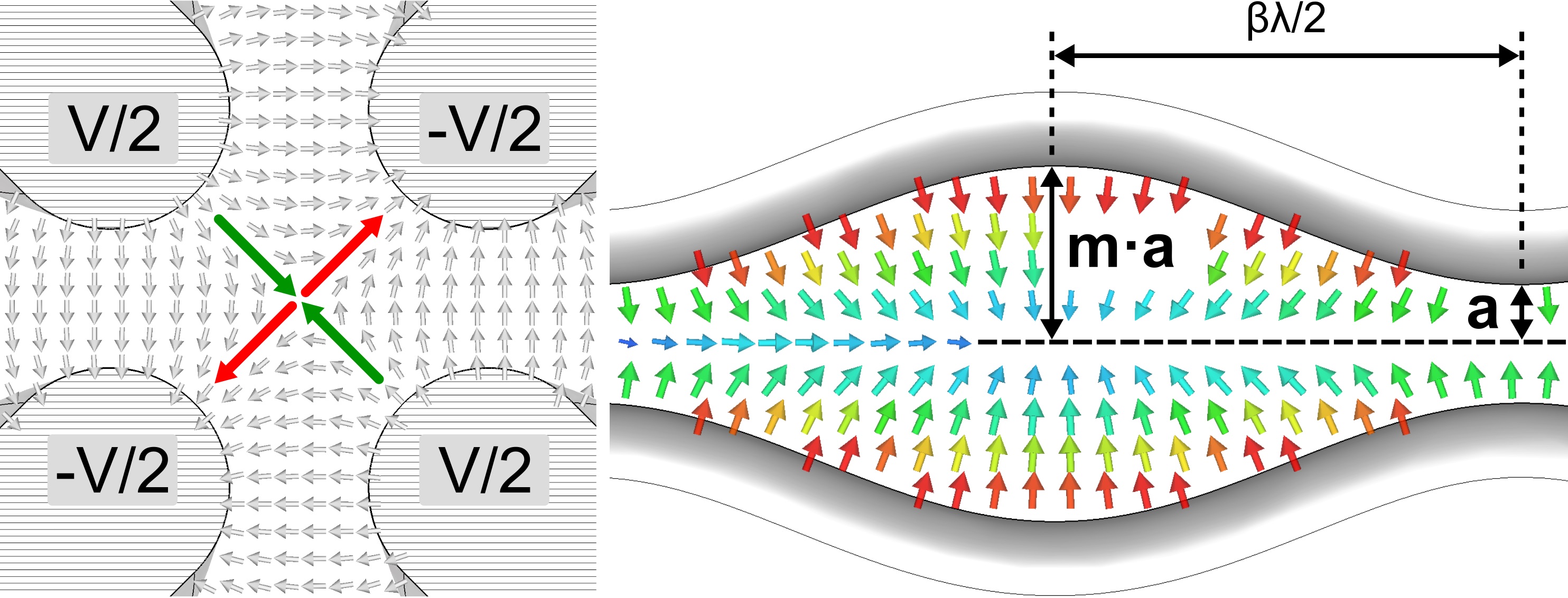
Figure 1: A single RFQ cell with electric fields in quasistatic approximation. Left: Front view. The green arrows indicate the focusing of the charged particle beam and the red arrows the defocusing. Right: Side view with cell geometry parameters shown and electric field indicated by arrows. From [16].

Here, we focus on the SM for the RFQ and how we can improve the neural network (NN) training and performance using the highly efficient Julia programming language [17]. Fully-connected neural networks have been rigorously proven to be able to predict any outcome given enough representative input data, as long as the NN has had sufficient training time and a sufficient number of parameters [18], making them a viable starting point for the development of an RFQ SM. The working principle of an RFQ and the generation of training data for the SM were discussed in detail in Koser et al. [16]. We briefly summarize them in Section I.1, and Section II.1, respectively. Then we discuss the input data and results of an expanded hyper-parameter scan before making recommendations for further studies.

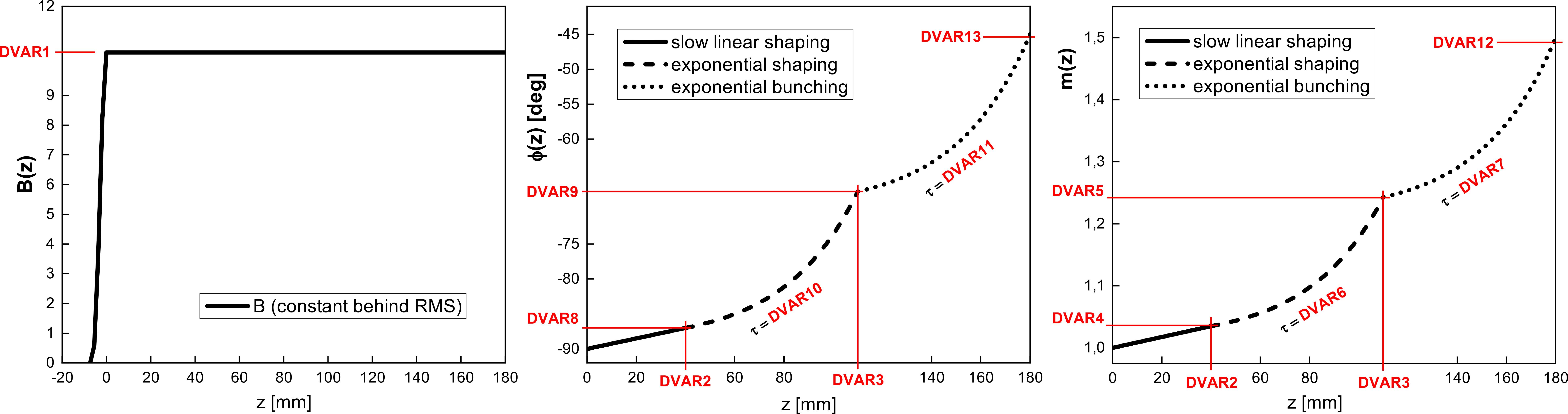
Figure 2: The three main cell parameters (focusing function $B$, phase $\Phi$, and modulation $m$), parametrized along the length of the RFQ by thirteen DVARs. From [16].

I.1 The Radio-Frequency Quadrupole

An RFQ is a multi-purpose linear particle accelerator structure able to bunch and accelerate a high current ion beam, while keeping it tightly focused. The IsoDAR RFQ is discussed in detail elsewhere [19, 20], here we will give a brief summary of aspects pertaining to data generation for the NN. In an RFQ, an oscillating electric field is generated between four so-called vanes (or rods). The transverse arrangement can be seen in Figure 1, left. The resulting forces act focusing on the beam. In the longitudinal direction, a modulation is machined onto the RFQ to provide an additional z-directed field component for acceleration and bunching. Half a period of this approximately sinusoidal modulation is called one cell of length $\beta\cdot\lambda/2$, where $\beta$ is beam velocity devided by the speed of light and $\lambda$ is the wavelength corresponding to the frequency of the electromagnetic wave driving the RFQ. Typical RFQs comprise tens to hundreds of such cells, each defined by three main parameters (the focusing strength $B$, the phase $\Phi$, and the modulation $m$). To optimize an RFQ, the parameters of each cell have to be fine-tuned to yield the highest transmission and desired beam output quantities. In this paper, we call the RFQ parameters design variables (DVARs) and the beam output parameters objectives (OBJs).

I.2 The Julia language

Julia is an open-source dynamically typed programming language with significant performance improvements over other languages common in scientific computing like Python and Matlab [17]. Julia’s computational efficiency is especially apparent when performing costly calculations like neural network training, motivating our use of the language throughout this analysis and allowing for straightforward implementation of multithreading and distributed computing to facilitate the completion of expensive computational tasks. In addition, Julia has built-in support for GPU programming using CUDA.jl [21, 22].

II Methodology

II.1 Data generation

We used the same dataset that we generated for our previous publication [16]. In summary, the set comprises 217,292 samples each containing 14 RFQ design variables (DVARs), features which are used to configure an RFQ through which beam dynamics are simulated to create the 6 objectives (OBJs). The objectives include beam transmission, output energy, RFQ length, and beam emittance (three OBJs for the three spatial dimensions).

To reduce the number of input parameters per sample from several hundred when using each individual cell’s three parameters to 14, Koser et al. devised a parametrization scheme [16] that is schematically depicted in Figure 2, wherein the RFQ is divided into sections longitudinally, and it is assumed that the cell parameters each follow either a linear or exponential distribution, described by the 14 DVARs.

II.2 Data preprocessing

Unlike [16], we decorrelate the data set, as some variables have values that directly affect the values of others. In particular, for some upper bounds $u_{i}$ and buffers $\eta_{i}$, $i\in\{3,5,9,12,13\}$, for a sample $j$ of the feature space hypercube:

$$\begin{split}\mathtt{DVAR3}_{j}&\sim\textrm{Uniform}(\mathtt{DVAR2}_{j}+\eta_{3},u_{3})\\ \mathtt{DVAR5}_{j}&\sim\textrm{Uniform}(\mathtt{DVAR4}_{j}+\eta_{5},u_{5})\\ \mathtt{DVAR9}_{j}&\sim\textrm{Uniform}(\mathtt{DVAR8}_{j}+\eta_{9},u_{9})\\ \mathtt{DVAR12}_{j}&\sim\textrm{Uniform}(\mathtt{DVAR5}_{j}+\eta_{12},u_{12})\\ \mathtt{DVAR13}_{j}&\sim\textrm{Uniform}(\mathtt{DVAR9}_{j}+\eta_{13},u_{13})\end{split}$$ (1)

Design variables like DVAR3 are not uniformly distributed. We can introduce a variable $\texttt{DVAR3}^{\prime}$ that is uniformly distributed according to the following transformation of $\texttt{DVAR2},\texttt{DVAR3}$, and constants:

$$\mathtt{DVAR3}^{\prime}_{j}=\frac{\mathtt{DVAR3}_{j}-(\mathtt{DVAR2}_{j}+\eta_{3})}{u_{3}-(\mathtt{DVAR2}_{j}+\eta_{3})}$$ (2)

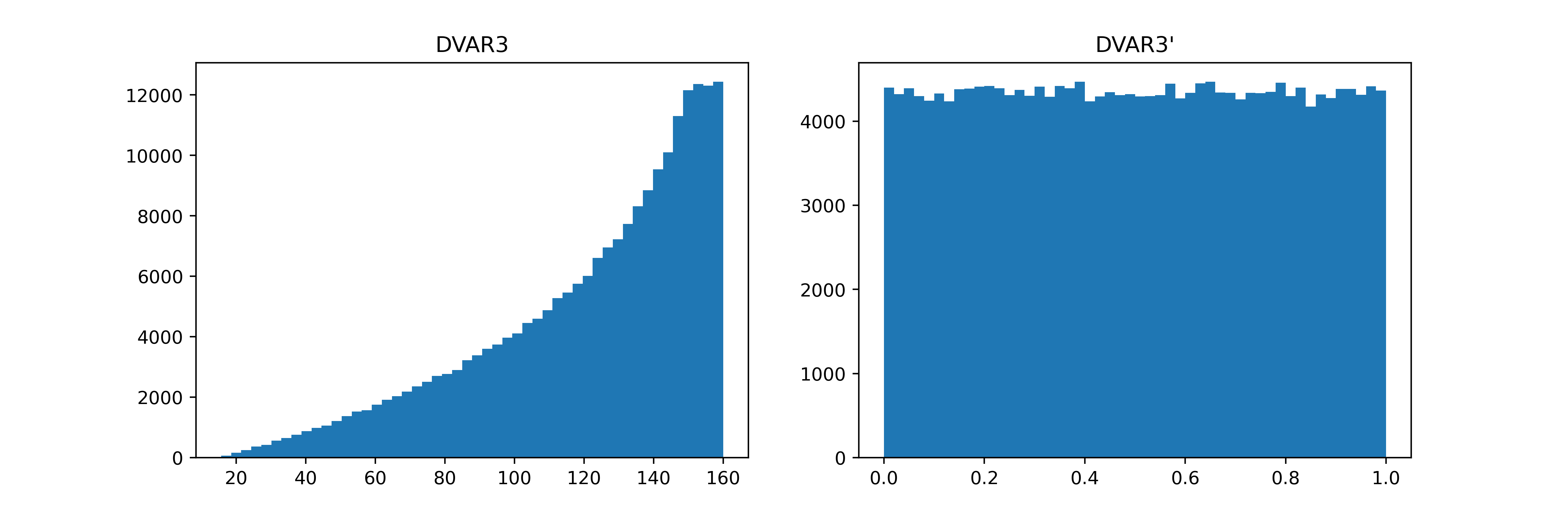
Figure 6: Histograms of the unscaled (left) and transformed (right) DVAR3. The transformation is outlined in equation 2.

And likewise for the remaining correlated features. A side-by-side comparison of distributions of DVAR3 and the transformed DVAR3’ is shown in Figure 6 in Appendix A.

Correlation matrices for the 14 design variables before and after the decorrelating transformation of necessary DVARs are shown in Figure 3. Each feature was later scaled to have minimum $-1$ and maximum $+1$

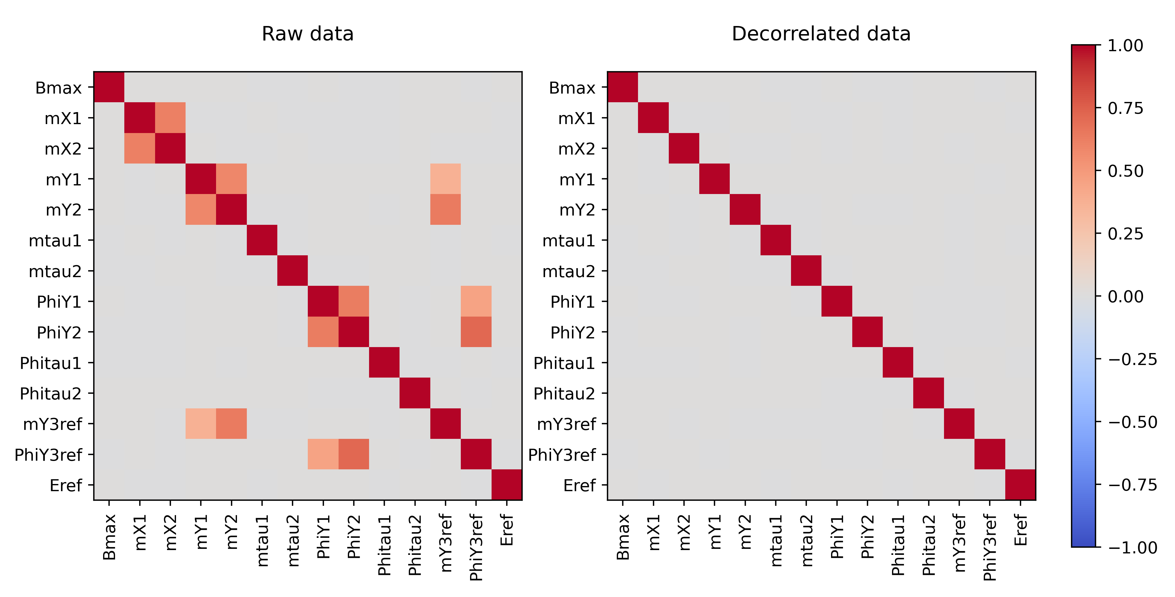
Figure 3: Correlation matrices for raw and decorrelated feature data.

To assess the impact of decorrelating data on NN training and performance, we trained two identical neural networks on both correlated and decorrelated scaled datasets. The loss curves are plotted for each of these datasets and are shown in Figure 4. We observed no significant difference in the training times or prediction accuracy between these two NNs. Because we consider it good practice, we use the uncorrelated data for the remainder of the study.

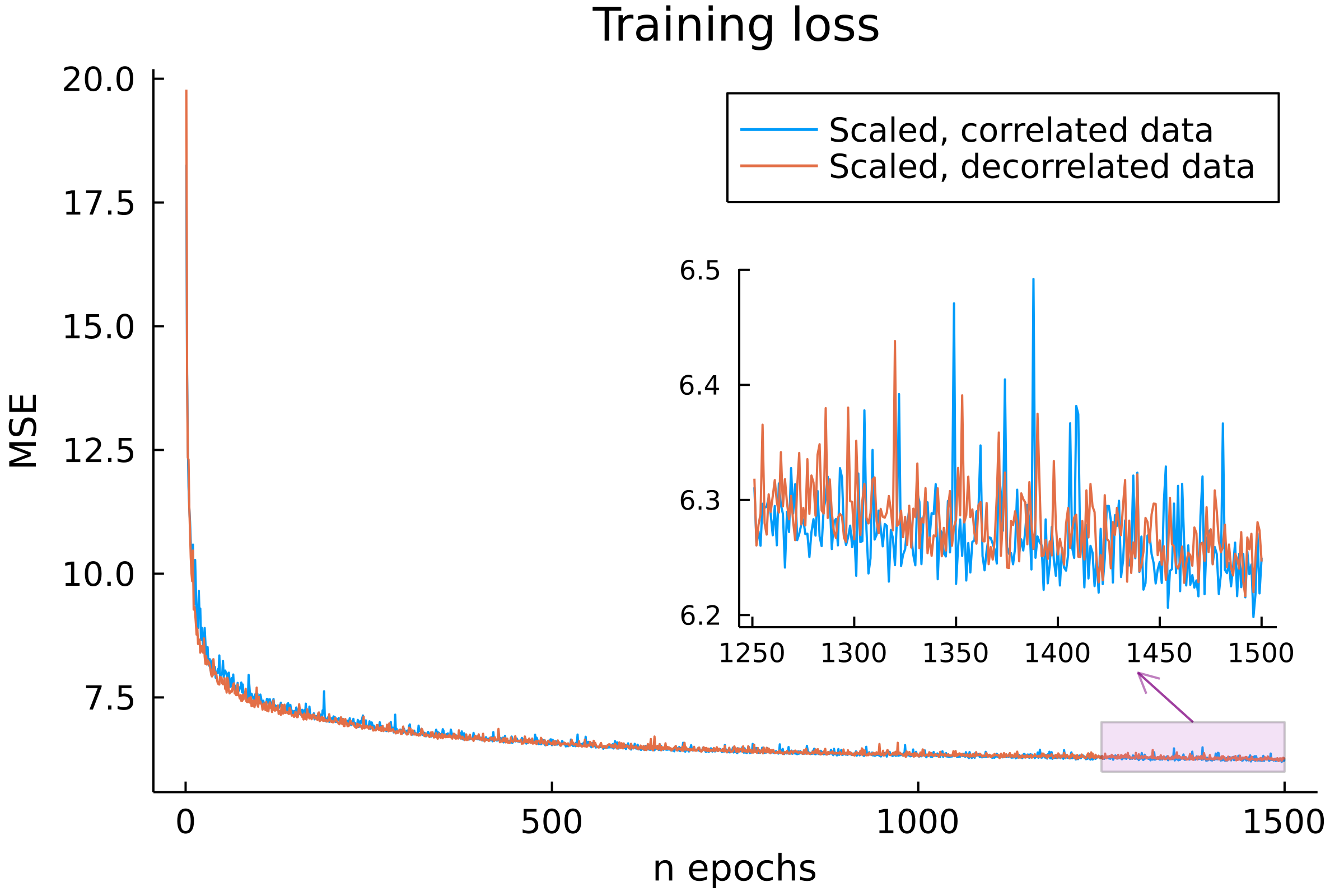
Figure 4: Training loss curves for identical neural networks trained on scaled and scaled/decorrelated datasets. A zoomed-in plot of the last 250 epochs of training is inset. There were no significant differences in NN training time or performance.

II.3 Feasibility of hyperparameter scans with Julia

We demonstrate Julia’s effectiveness for performing hyperparameter searches by doing grid searches varying model architecture hyperparameters, namely, NN width and depth. We hold batch size, learning rate, and activation functions constant for this study but plan to expand our searches to these hyperparameters, as well. Scanned NN hyperparameters are summarized in Table 1. Neural network training was performed primarily using the Flux.jl package, an open-source Julia library used for training deep ML models [23][24]. NNs of different architectures were trained in parallel to reduce script runtime.

Data was split into training and test sets (of proportions 80% and 20%, respectively). The test set was withheld from any analysis for the entirety of the scan. We used the MLUtils.jl package [25] to perform 5-fold cross-validation, where each neural network was trained on an 80% subsample of the training data, with the remaining 20% used as a validation dataset to compute out-of-sample model performance. NNs were not trained on this smaller subset of data. Cross-validation allows us to estimate statistical significance by performing repeated trails to estimate a NN configuration’s out-of-sample prediction accuracy.

Results from [16] indicate that neural networks trained with larger batch sizes were preferred, as demonstrated by the hyperparameter search’s choice of a batch size of 256, the largest in the range studied. While larger batch sizes may be preferred in principle to show NNs more data per training step, computational limits make their implementation difficult in practice [26]. The use of Julia allows us to feasibly consider training neural networks with larger batch sizes in a more reasonable amount of time. Hence, we choose to hold batch size constant at 1024, outside of the range of that explored by [16].

Each neural network was constructed using a sigmoid activation function. The Flux.jl ADAM [27] optimizer was used to perform stochastic gradient descent in neural network training, using the default learning rate of $\eta=0.001$. All neural networks were trained for 2500 epochs, which appeared experimentally to be a reasonable threshold for convergence. Future work will incorporate more sophisticated early stopping procedures to aid scan runtime.

Hyperparameter	Value(s) scanned
NN depth	4, 5, 6
NN width	50, 75, 100
Batchsize	1024
Learning rate	0.001
Activation function	Sigmoid

Table 1: Values chosen for feasibility study of hyperparameter search in Julia.

II.4 Reporting

Neural network performance is determined by computing $R^{2}$ scores and Mean Absolute Percent Errors (MAPEs). We compute $R^{2}$ scores between predicted and true values of the output variables and average the results together to calculate “aggregate $R^{2}$” scores. We note that this metric does not encompass the prediction accuracy of a given model on all objectives simultaneously, so when appropriate, we report $R^{2}$ scores of each object variable separately.

III Results

Results of the preliminary hyperparameter scan we performed on the full RFQ dataset described in Section II.1 are reported in Table 2, which gives the validation-set $R^{2}$ means and standard deviations across the 5 folds of the cross validation. The aggregate training set loss for the last 1000 epochs of training are showed in Figure 5. MAPEs of model predictions for the NN with depth 6 and width 100 are summarized in Table 3 where we draw a comparison to [16].

	Depth 4	Depth 5	Depth 6
Width 50	$0.9808\pm 0.000164$	$0.9809\pm 0.000197$	$0.9808\pm 0.000138$
Width 75	$0.9798\pm 0.000178$	$0.9795\pm 0.000095$	$0.9792\pm 0.000235$
Width 100	$0.9804\pm 0.000172$	$0.9803\pm 0.000163$	$0.9801\pm 0.000243$

Table 2: Aggregated validation set $R^{2}$ scores. This $R^{2}$ score is computed across all objective variables, but is not representative of the prediction accuracy of individual objectives. The $R^{2}$ score for each objective for each NN architecture is shown in Appendix C.

Objective label	Objective variable	This work	Koser, et al. [16]
OBJ1	Transmission [%]	$1.7\%$	$2.4\%$
OBJ2	Output energy [MeV]	$1.8\%$	$1.9\%$
OBJ3	RFQ length [cm]	$1.3\%$	$2.0\%$
OBJ4	Longitudinal $\epsilon$ [MeV deg]	$4.8\%$	$8.2\%$
OBJ5	$\epsilon_{x}$ [cm mrad]	$11.7\%$	$12.8\%$
OBJ6	$\epsilon_{y}$ [cm mrad]	$11.5\%$	$12.5\%$

Table 3: MAPE of NN with width 100 and depth 6 by response compared to previous analysis.

The reduction of MAPEs for some of the OBJs is encouraging. However, the improvement in others was relatively small. To make recommendations for future studies, we also tested the “sandbox” problem described in [16], the so called FODO cell, which is a simple magnetic focusing device used frequently in particle accelerators.

We freshly generated the data for this example using the particle-in-cell code OPAL [28]. The DVARs and limits thereof are listed in Table 5 in Appendix B. We used a sample size of 2000. For training we used three fully-connected layers each of width $25$ with sigmoid activation functions, and trained the neural network using a Mean Squared Error loss function with the Flux.jl ADAM optimizer with a default learning rate of $\eta=0.001$. We used a batch size of 64. Out-of-sample MAPEs are reported in Table 4. The MAPEs are comparable to the ones reported previously [16], corroborating the notion that the FODO is a good test bench for SM generation for RFQs as it exhibits similar difficulties.

Objective variable	This work
Energy spread	$0.85\%$
$\epsilon_{x}$	$7.5\%$
$\epsilon_{y}$	$9.0\%$
RMS-$z$	$1.8\%$
RMS-$x$	$1.5\%$
RMS-$y$	$3.0\%$

Table 4: MAPE of NN with width 25 and depth 3 by response on toy FODO data. These MAPEs are comparable to previous analysis [16].

The final study we performed was to move training of the NN to the GPU. Here we used a Nvidia GeForce GTX 750 Ti with 2 GB of VRAM combined with an AMD FX(tm)-8320 eight core CPU. With a 500 epoch, 2-fold cross-validation of a NN with width = 100 and depth = 5, we saw an improvement of 28 % over the pure-CPU execution of the same Julia code, encouraging us to utilize GPUs for future training needs.

IV Discussion

This analysis demonstrates the effectiveness of Julia for use in performing rigorous hyperparameter searches for deep NN models to serve as surrogate models for RFQ-throughgoing beam dynamics. A particular advantage of Julia is that its high computational performance allows us to train neural networks with larger batch sizes more feasibly than an equivalent implementation in Python. Already, by training a series of neural networks with a batch size of 1024, we reduce the out-of-sample MAPE by as much as 45% for some objective variables. The out-of-sample MAPEs are improved for each of the objectives studied. We also note that a best practice moving forward is to continue to develop any future ML SMs by training on decorrelated data.

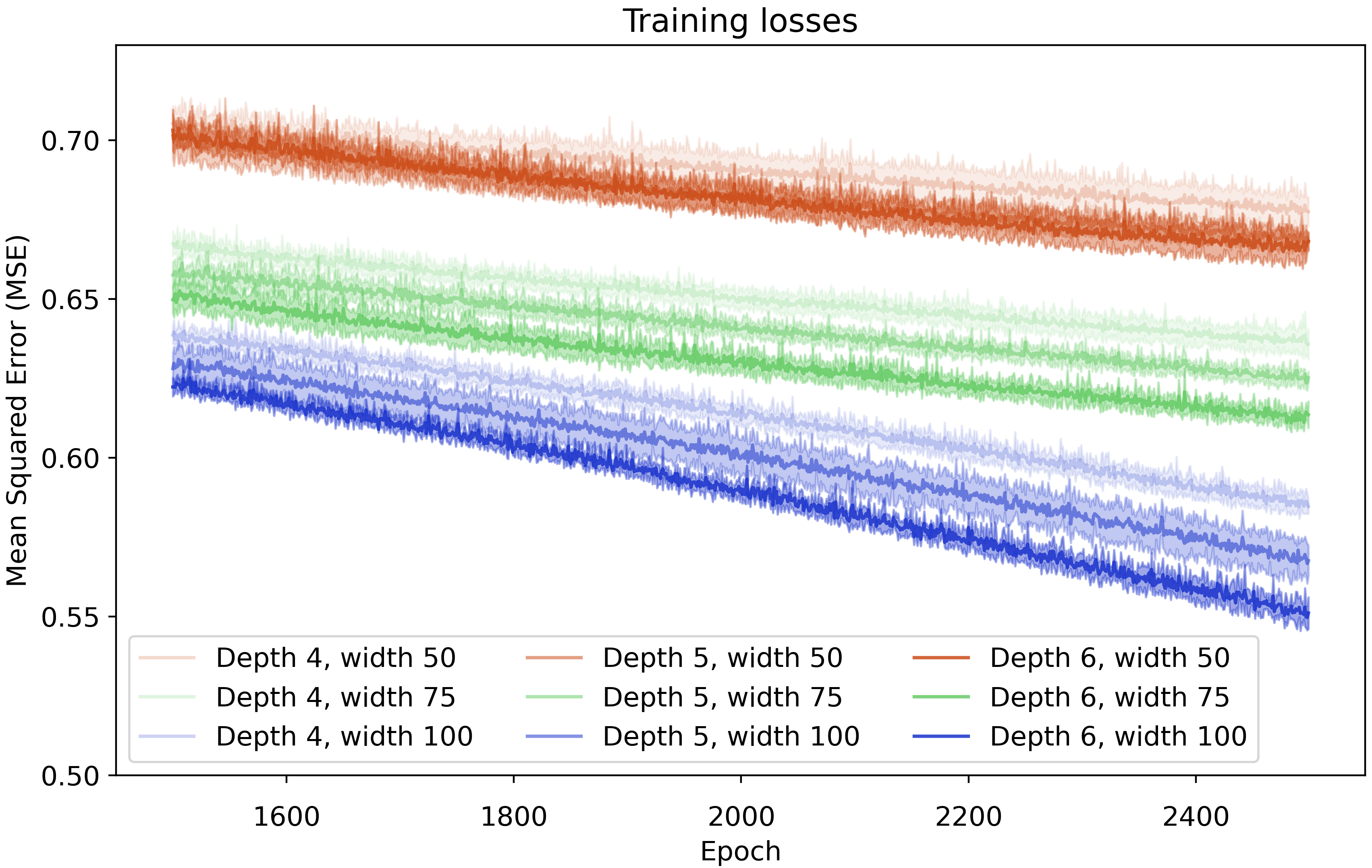
Figure 5: Last 1,000 epochs of training-set losses of neural networks trained during hyperparameter scan. The solid line in the center of each curve represents the mean of the 5 folds’ loss function values at the same epoch. We shade above and below the mean by one standard deviation.

We have noticed that many of the models are overfitting. Significant boosts in training losses as shown in Figure 5 correspond to no significant improvement in out-of-sample $R^{2}$ shown in Table 2. We would expect out-of-sample $R^{2}$ to be higher as the number of model parameters increases, which is not what we observe. We note however that this pattern is not consistent across out-of-sample prediction accuracy for all objectives: see Appendix C. For example, OBJ5 seemed to prefer a neural network of width 100 and depth 5, while OBJ2 seemed to prefer a much simpler neural network of width 50 and depth 5.

The appearance of overtraining in the small subset of NNs studied, and the significant improvements in MAPE for top-performing NNs in this work over [16], lead us to make the following recommendations:

1. Include dropout layers. Dropout layers introduce regularization by randomly sending the weights of a subset of nodes of the neural network to zero, which has been shown as an effective remedy to overfitting [29]. In future work, we aim to demonstrate that the inclusion of dropout layers allows us to introduce more parameters into our neural networks without fear of overfitting, aiding in out-of-sample performance.

2. Expand the hyperparameter search to include larger batch sizes. Increasing the batch size for NN training has already proven promising, and the use of high-performance computing with Julia (such as GPU computing) make larger batch sizes possible.

3. Explore different neural network architectures for different objectives. Based on the NNs studied in this preliminary analysis, we conclude that different objectives may not respond simiarly to different NN architectures (indicated explicitly in the out-of-sample $R^{2}$ scores for each objective, see Appendix C. We can feasibly run hyperparameter scans for NNs aiming to predict one (or perhaps some subset of) objective(s) for additional boosts in performance. We are especially interested in implementing such models for the poorest-performing objectives, namely, $x$- and $y$-emittances.

4. Use more efficient hyperparameter search techniques. While brute force hyperparameter grid searches are by nature exhaustive, they are computationally expensive. Employing Bayesian hyperparameter optimization procedures or genetic algorithms to identify top-performing NNs may prove useful for shortening script runtime and allowing us better resolution in finetuning neural network architecture for best prediction accuracy.

5. Explore surrogate model architectures beyond fully-connected neural networks and summary statistic inputs. We emphasize that multivariate regressive tasks are not limited to just fully-connected neural networks, or that the only way to develop an RFQ SM is by feeding the exact same 14 design variables that we reference in this study. One possibility is to build a convolutional neural network (CNN) that takes as inputs multidimensional images of the beam phase space, intuition being a more granular picture of the beam rather than just the beam’s summary statistics.

V Conclusion

The utility of Julia for the development of SMs cannot be understated. We were particularly impressed with how easy Julia is to use, and how well it handles computationally difficult tasks like training series of NNs with large batch sizes. We anticipate that the use of Julia to train neural networks on GPUs will make this even faster. Above all, use of Julia makes more expensive computational tasks feasible, allowing us to extend our hyperparameter searches to continue to find SMs that can one day reliably be used for RFQ optimization.

Appendix A Histograms of the transformed design variable

Appendix B FODO DVARs and limits

Design variable label	Design variable	Lower bound	Upper bound
DVAR1	Correlation x-px	-1	1
DVAR2	Correlation y-py	-1	1
DVAR3	Beam current (mA)	1	10
DVAR4	K1 of Quadrupole 1 (1/m2)	5	40
DVAR5	K1 of Quadrupole 2 (1/m2)	5	40
DVAR6	1-$\sigma$ beam length in z (m)	0.001	0.1
DVAR6	1-$\sigma$ beam length in x (m)	0.01	0.05
DVAR6	1-$\sigma$ beam length in y (m)	0.01	0.05

Table 5: DVARs for the FODO cell test.

Appendix C Out-of-sample $R^{2}$ scores for scanned neural networks

For tables 6 to 11, cells corresponding to neural network architectures with the highest $R^{2}$ scores are shown in bold. This points to the fact that different neural network architectures may be better equipped to predict different output variables. For neural network with equal validation-set mean $R^{2}$, we use the lowest $R^{2}$ standard deviation as a tiebreaker.

	Depth 4	Depth 5	Depth 6
Width 50	$0.9941\pm 0.000556$	$0.9957\pm 0.000315$	$\mathbf{0.9958\pm 0.000167}$
Width 75	$0.9946\pm 0.000288$	$0.9956\pm 0.000284$	$0.9958\pm 0.000277$
Width 100	$0.994\pm 0.000163$	$0.9956\pm 0.000668$	$0.9955\pm 0.000263$

Table 6: Validation set $R^{2}$ scores for OBJ1 (transmission).

	Depth 4	Depth 5	Depth 6
Width 50	$0.9452\pm 0.000426$	$\mathbf{0.9456\pm 0.000401}$	$0.9443\pm 0.000378$
Width 75	$0.9454\pm 0.000383$	$0.9452\pm 0.000232$	$0.9442\pm 0.000308$
Width 100	$0.945\pm 0.000602$	$0.9451\pm 0.000273$	$0.9436\pm 0.000429$

Table 7: Validation set $R^{2}$ scores for OBJ2 (output energy).

	Depth 4	Depth 5	Depth 6
Width 50	$0.9958\pm 0.000565$	$\mathbf{0.9966\pm 0.000471}$	$0.9961\pm 0.00039$
Width 75	$0.9958\pm 0.000519$	$0.9963\pm 0.000436$	$0.9959\pm 0.000434$
Width 100	$0.9954\pm 0.000327$	$0.9963\pm 0.000374$	$0.9953\pm 0.000361$

Table 8: Validation set $R^{2}$ scores for OBJ3 (RFQ length).

	Depth 4	Depth 5	Depth 6
Width 50	$0.8924\pm 0.0298$	$0.91\pm 0.03$	$0.9075\pm 0.03$
Width 75	$0.8927\pm 0.0301$	$\mathbf{0.9121\pm 0.0307}$	$0.9061\pm 0.0315$
Width 100	$0.8934\pm 0.0309$	$0.9105\pm 0.0329$	$0.9009\pm 0.0313$

Table 9: Validation set $R^{2}$ scores for OBJ4 (longitudinal emittance).

	Depth 4	Depth 5	Depth 6
Width 50	$0.843\pm 0.00312$	$0.8483\pm 0.00281$	$0.8385\pm 0.00109$
Width 75	$0.8453\pm 0.00305$	$0.8495\pm 0.00313$	$0.8353\pm 0.00219$
Width 100	$0.8466\pm 0.003$	$\mathbf{0.8498\pm 0.00291}$	$0.8322\pm 0.0034$

Table 10: Validation set $R^{2}$ scores for OBJ5 ($x$-emittance).

	Depth 4	Depth 5	Depth 6
Width 50	$0.8425\pm 0.00273$	$0.8463\pm 0.00193$	$0.8359\pm 0.00145$
Width 75	$0.8437\pm 0.00244$	$\mathbf{0.848\pm 0.00207}$	$0.8324\pm 0.00162$
Width 100	$0.8447\pm 0.0027$	$0.8474\pm 0.00219$	$0.8309\pm 0.00208$

Table 11: Validation set $R^{2}$ scores for OBJ6 ($y$-emittance).