Bagging in overparameterized learning:
Risk characterization and risk monotonization
Abstract
Bagging is a commonly used ensemble technique in statistics and machine learning to improve the performance of prediction procedures. In this paper, we study the prediction risk of variants of bagged predictors under the proportional asymptotics regime, in which the ratio of the number of features to the number of observations converges to a constant. Specifically, we propose a general strategy to analyze the prediction risk under squared error loss of bagged predictors using classical results on simple random sampling. Specializing the strategy, we derive the exact asymptotic risk of the bagged ridge and ridgeless predictors with an arbitrary number of bags under a well-specified linear model with arbitrary feature covariance matrices and signal vectors. Furthermore, we prescribe a generic cross-validation procedure to select the optimal subsample size for bagging and discuss its utility to eliminate the non-monotonic behavior of the limiting risk in the sample size (i.e., double or multiple descents). In demonstrating the proposed procedure for bagged ridge and ridgeless predictors, we thoroughly investigate the oracle properties of the optimal subsample size and provide an in-depth comparison between different bagging variants.
Contents
\@afterheading\@starttoc
toc
1 Introduction
Modern machine learning models often use a large number of parameters relative to the number of observations. In this regime, several commonly used procedures exhibit a peculiar risk behavior, which is referred to as double or multiple descents in the risk profile (Belkin et al.,, 2019; Zhang et al.,, 2017, 2021). The precise nature of the double or multiple descent behavior in the generalization error has been studied for various procedures: e.g., linear regression (Belkin et al.,, 2020; Muthukumar et al.,, 2020; Hastie et al.,, 2022), logistic regression (Deng et al.,, 2022), random features regression (Mei and Montanari,, 2022), kernel regression (Liu et al.,, 2021), among others. We refer the readers to the survey papers by Bartlett et al., (2021); Belkin, (2021); Dar et al., (2021) for a more comprehensive review and other related references. In these cases, the asymptotic prediction risk behavior is often studied as a function of the data aspect ratio (the ratio of the number of parameters/features to the number of observations). The double descent behavior refers to the phenomenon where the (asymptotic) risk of a sequence of predictors first increases as a function of the aspect ratio, peaks at a certain point (or diverges to infinity), and then decreases with the aspect ratio. From a traditional statistical point of view, the desirable behavior as a function of aspect ratio is not immediately obvious. We can, however, reformulate this behavior as a function of , in terms of the observation size with a fixed ; imagine a large but fixed and changing from to . In this reformulation, the double descent behavior translates to a pattern in which the risk first decreases as increases, then increases, peaks at a certain point, and then decreases again with . This is a rather counter-intuitive and sub-optimal behavior for a prediction procedure. The least one would expect from a good prediction procedure is that it yields better performance with more information (i.e., more data). However, the aforementioned works show that many commonly used predictors may not exhibit such “good” behavior. Simply put, the non-monotonicity of the asymptotic risk as a function of the number of observations or the limiting aspect ratio implies that more data may hurt generalization (Nakkiran,, 2019).
Several ad hoc regularization techniques have been proposed in the literature to mitigate the double/multiple descent behaviors. Most of these methods are trial-and-error in nature in the sense that they do not directly target monotonizing the asymptotic risk but instead try a modification and check that it yields a monotonic risk. The recent work of Patil et al., 2022b introduces a generic cross-validation framework that directly addresses the problem and yields a modification of any given prediction procedure that provably monotonizes the risk. In a nutshell, the method works by training the predictor on subsets of the full data (with different subset sizes) and picking the optimal subset size based on the estimated prediction risk computed using testing data. Intuitively, it is clear that this yields a prediction procedure whose risk is a decreasing function of the observation size. In the proportional asymptotic regime, where as , the paper proves that this strategy returns a prediction procedure whose asymptotic risk is monotonically increasing in . The paper theoretically analyzes the case where only one subset is used for each subset size and illustrates via numerical simulations that using multiple subsets of the data of the same size (i.e., subsampling) can yield better prediction performance in addition to monotonizing the risk profile. Note that averaging a predictor computed on different subsets of the data of the same size is referred to in the literature as subagging, a variant of the classical bagging (bootstrap aggregation) proposed by Breiman, (1996). The focus of the current paper is to analyze the properties of bagged predictors in two directions (in the proportional asymptotics regime): (1) what is the asymptotic predictive risk of the bagged predictors with bags as a function of , and (2) does the cross-validated bagged predictor provably yield improvements over the predictor computed on full data and does it have a monotone risk profile (i.e., the asymptotic risk is a monotonic function of )?
In this paper, we investigate several variants of bagging, including subagging as a special case. The second variant of bagging, which we call splagging (that stands for split-aggregating), is the same as the divide-and-conquer or the data-splitting approach (Rosenblatt and Nadler,, 2016; Banerjee et al.,, 2019). The divide-and-conquer approach is widely used in distributed learning, although not commonly featured in the bagging literature (Dobriban and Sheng,, 2020, 2021; Mücke et al.,, 2022). Formally, splagging splits the data into non-overlapping parts of equal size and averages the predictors trained on these non-overlapping parts. We refer to the equal size of each part of the data as subsample size. We use the same terminology for subagging also for the sake of simplicity. Using classical results from survey sampling and some simple lemmas about almost sure convergence, we are able to analyze the behavior of subagged and splagged predictors666A note on terminology for the paper: when referring to subagging and splagging together, we use the generic term bagging. Similarly, when referring to subagged and splagged predictors together, we simply say bagged predictors. with bags for arbitrary prediction procedures and general . In fact, we show that the asymptotic risk of bagged predictors for general (or simply, -bagged predictor) can be written in terms of the asymptotic risks of bagged predictors with and . Rather interestingly, we prove that the -bagged predictor’s finite sample predictive risk is uniformly close to its asymptotic limit over all . These results are established in a model-agnostic setting and do not require the proportional asymptotic regime. Deriving the asymptotic risk behavior of bagged predictors with and has to be done on a case-by-case basis, which we perform for ridge and ridgeless prediction procedures. In the context of bagging for general predictors, we further analyze the cross-validation procedure with -bagged predictors for arbitrary to select the “best” subsample size for both subagging and splagging. These results show that subagging and splagging for any outperform the predictor computed on the full data. We further present conditions under which the cross-validated predictor with -bagged predictors has an asymptotic risk monotone in the aspect ratio. Specializing these results to the ridge and ridgeless predictors leads to somewhat surprising results connecting subagging to optimal ridge regression as well as the advantages of interpolation.
Before proceeding to discuss our specific contributions, we pause to highlight the two most significant take-away messages from our work. These messages hold under a well-specified linear model, where the features possess an arbitrary covariance structure, and the response depends on an arbitrary signal vector, both of which are subject to certain bounded norm regularity constraints.
-
(T0)
Subagging and splagging (the data-splitting approach) of the ridge and ridgeless predictors, when properly tuned, can significantly improve the prediction risks of these standalone predictors trained on the full data. This improvement is most pronounced near the interpolation threshold. Importantly, subagging always outperforms splagging. See the left panel of Figure 1 for a numerical illustration and Proposition 4.6 for a formal statement of this result.
-
(T0)
A model-agnostic algorithm exists to tune the subsample size for subagging. This algorithm produces a predictor whose risk matches that of the oracle-tuned subagged predictor. Notably, the oracle-tuned subsample size for the ridgeless predictor is always smaller than the number of features. As a result, subagged ridgeless interpolators always outperform subagged least squares, even when the full data has more observations than the number of features. The same observation holds true for splagging whenever it provides an improvement. See the right panel of Figure 1 for numerical illustrations and Proposition 4.7 for formal statements of this result.
Intuitively, although bagging may induce bias due to subsampling, it can significantly reduce the prediction risk by reducing the variance for a suitably chosen subsample size that is smaller than the feature size. This tradeoff arises because of the different rates at which the bias and variance of the ridgeless predictor increase near the interpolation threshold. This advantage of interpolation or overparameterization is distinct from other benefits discussed in the literature, such as self-induced regularization (Bartlett et al.,, 2021).
1.1 Summary of main results
Below we provide a summary of the main results of this paper.
-
1.
General predictors. In Section 2, we formulate a generic strategy for analyzing the limiting squared data conditional risk (expected squared error on a future data point, conditional on the full data) of general -bagged predictors, showing that the existence of the limiting risk for and implies the existence of the limiting risk for every . Moreover, we show that the limiting risk of the -bagged predictor can be written as a linear combination of the limiting risks of -bagged predictors with and . Interestingly, the same strategy also works for analyzing the limit of the subsample conditional risk, which considers conditioning on both the full data and the randomly drawn subsamples. See Theorem 2.9 for a formal statement. In this general framework, Theorem 2.9 implies that both the data conditional and subsample conditional risks are asymptotically monotone in the number of bags . Moreover, for general strongly convex and smooth loss functions, we can sandwich the risks between quantities of the form , for some fixed random variables and (Proposition 2.6).
-
2.
Ridge and ridgeless predictors. In Section 3, we specialize the aforementioned general strategy to characterize the data conditional and subsample conditional risks of -bagged ridge and ridgeless predictors. The results are formalized in Theorem 3.1 for subagging with and without replacement, and Theorem 3.6 for splagging without replacement. All these results assume a well-specified linear model, with an arbitrary covariance matrix for the features and an arbitrary signal vector. Notably, we assume neither Gaussian features nor isotropic features nor a randomly generated signal. These results reveal that for the three aforementioned bagging strategies, the bias and variance risk components are non-increasing in the number of bags .
-
3.
Cross-validation. In Section 4, we develop a generic cross-validation strategy to select the optimal subsample or split size (or equivalently, the subsample aspect ratio) and present a general result to understand the limiting risks of cross-validated predictors. Our theoretical results provide a way to verify the monotonicity of the limiting risk of the cross-validated predictor in terms of the limiting data aspect ratio (Theorem 4.1). In Section 4.2, we specialize in the cross-validated ridge and ridgeless predictors to obtain the optimal subsample aspect ratio for every (Theorem 4.5). Moreover, when optimizing over both the subsample aspect ratio and the number of bags, we show that optimal subagging always outperforms optimal splagging (Proposition 4.6). Rather surprisingly, in our investigation of the oracle choice of the subsample size for optimal subagging with , we find that the subsample ratio is always large than one (Proposition 4.7). In Section 5, we also show optimally-tuned subbaged ridgeless predictor yields the same prediction risk as the optimal ridge predictor for isotropic features (Theorem 5.3).
From a technical perspective, during the course of our risk analysis of the bagged ridge and ridgeless predictors, we derive novel deterministic equivalents for ridge resolvents with random Tikhonov-type regularization. We extend ideas of conditional asymptotic equivalents and related calculus, which may be of independent interest. See Appendix S.7, and in particular Section S.7.3.2.
1.2 Related work
The risk non-monotonicity of commonly used predictors has been well documented in the literature. For instance, a recent line of work by Belkin et al., (2019); Viering et al., (2019); Nakkiran, (2019); Loog et al., (2019), among others, illustrates the non-monotonic risk behavior of several prediction procedures. See also the survey papers by Belkin, (2021); Bartlett et al., (2021); Dar et al., (2021); Loog et al., (2020) for other related references. As highlighted by Loog et al., (2020), the phenomenon of multiple descents can be traced back to empirical findings in the 1990s, including earlier papers by Vallet et al., (1989); Hertz et al., (1989); Opper et al., (1990); Hansen, (1993); Barber et al., (1995); Duin, (1995); Opper, (1995); Opper and Kinzel, (1996); Raudys and Duin, (1998), among others.
Since non-monotonic risk leads to suboptimal use of the data, several methods have been proposed that modify a given (class of) prediction procedure(s) to construct a new prediction procedure with a monotonic risk profile. In particular, Nakkiran et al., (2021) investigates the role of optimal tuning in the context of ridge regression and demonstrates that the optimally-tuned regularization achieves monotonic generalization performance for a class of linear models under isotropic design. Mhammedi, (2021) provides an algorithm to monotonize the risk profile for bounded loss functions. Patil et al., 2022b propose a general framework to monotonize the prediction risk for general predictors under both bounded and unbounded loss functions, using cross-validation. The paper also empirically shows that bagging can further improve the performance of the predictors while achieving a monotonized risk profile. In this paper, we characterize the risk behavior of bagging, which was left as an open direction in Patil et al., 2022b . Below we provide a brief overview of the literature pertaining to bagging and its relation to our work.
Ensemble methods are widely used in machine learning and statistics and combine several weak predictors to produce one powerful predictor. One important class of ensemble methods is bagging (Breiman,, 1996; Bühlmann and Yu,, 2002), and its variants, such as subagging (Bühlmann and Yu,, 2002), that operate by averaging predictors trained on independent subsamples of the data. Numerous empirical studies have demonstrated that bagging leads to significant improvements in predictive performance (Breiman,, 1996; Strobl et al.,, 2009; Fernández-Delgado et al.,, 2014). However, the theoretical analysis of bagging has primarily focused on smooth predictors (predictors that are smooth functions of the empirical data distribution); see Buja and Stuetzle, (2006); Friedman and Hall, (2007). For some work on bagging for non-parametric estimators, see Hall and Samworth, (2005); Samworth, (2012); Wu et al., (2021); Bühlmann and Yu, (2002); Athey et al., (2019). In addition to sample-wise bagging, bagging over linear combinations of features has also been considered in Lopes et al., (2011); Srivastava et al., (2016); Cannings and Samworth, (2017). This approach broadly falls under the umbrella of feature side sketching; we refer readers to Wang et al., (2017); Derezinski et al., (2020); Lopes et al., (2018); Dereziński, (2023); LeJeune et al., (2022); Patil and LeJeune, (2023), among others, for related results and further references.
Bagging in the proportional asymptotic regime has also been considered in the literature. LeJeune et al., (2020) study subagging of both features and observations and derive the limiting risk of the resulting subagged predictor. Dobriban and Sheng, (2020, 2021); Mücke et al., (2022) consider the divide-and-conquer approach, or splagging, and investigate their properties. These works are set in the context of distributed learning. Specifically, under proportional asymptotics, Dobriban and Sheng, (2020) derive the limiting mean squared error of the distributed ridge estimator in the underparameterized regime. On the other hand, Mücke et al., (2022) provide finite-sample upper bounds on the prediction risk for ridgeless regression in the overparameterized regime.
The closest works to ours are those of LeJeune et al., (2020) and Mücke et al., (2022). LeJeune et al., (2020) investigate bagged least squares predictor obtained by subsampling both features and observations in a Gaussian isotropic design. They impose a restriction on subsampling such that the final subsampled data always has more observations than the features (so that ordinary least squares are well-defined). Consequently, they do not allow for overparameterized subsampled datasets. Similar to our work, they also study the monotonicity of the asymptotic expected squared risk with respect to the number of bags in their restricted setting. Further, they study the best subsampling ratios for optimal asymptotic risk, but do not consider the question of how to select the best subsample size. The most significant difference between their work and ours is that we subsample observations, and they effectively subsample features, which is only appropriate under isotopic covariance. On the other hand, Mücke et al., (2022) consider splagging and provide finite-sample upper bounds on the bias and variance components of the squared prediction risk under the assumption of sub-Gaussian features. In contrast, our results do not assume sub-Gaussianity for either the feature or response distributions and only impose minimal bounded moment assumptions.
1.3 Organization
Below we provide an outline for the rest of the paper.
-
•
In Section 2, we provide risk decompositions conditional on both the full dataset and subsampled datasets for different bagging variants for general predictors. Based on the form of decompositions, we provide a series of reductions and a generic strategy for analyzing the squared prediction risk of general bagged predictors.
-
•
In Section 3, we give risk characterizations for bagging ridge and ridgeless predictors. We give results for both subagging with and without replacement, and splagging without replacement, and show monotonicities of the bias and variance components in the number of bags.
-
•
In Section 4, we prescribe a framework for monotonizing the risk profile of any given predictor based on cross-validation over subsample size. The result is then specialized to the ridge and ridgeless predictors. Furthermore, we compare the monotonized risk profiles of bagged ridgeless and ridge predictors.
-
•
In Section 5, we specialize our results for isotropic features and provide explicit analytic expressions for the risks of bagged ridgeless regression. In addition, we present the analysis of the optimal subsample size and the corresponding optimal bagged risk.
-
•
In Section 6, we conclude the paper by providing related questions for future work.
In the Supplement to this paper, we give a brief background on simple random sampling, provide proof of all the results, and present additional numerical illustrations. The organization structure for the Supplement is provided in the first section of the Supplement, which also gives an overview of the general notation employed throughout the paper. The source code for reproducing all the experimental illustrations in this paper can be found at: https://github.com/jaydu1/Overparameterized-Bagging/tree/main/bagging.
2 Bagging general predictors
In this section, we will describe different versions of subagged predictors. But first, let us define the index sets pertinent to our study. Fix any and any permutation . Define the sets and as follows:
| (1) |
Note that both the sets and technically need to be indexed by , but for notation convenience, we will not explicitly indicate the dependence on . The set represents the set of all subset choices from . There are many of them. The set , on the other hand, represents the set of indices in a non-overlapping split of into blocks of size . If we split randomly into different non-overlapping blocks each of size , then this corresponds to choosing a permutation randomly from the set of all permutations and splitting them in order. Finally, observe that for any permutation and .
2.1 Conditional risk decompositions
Suppose now represents a dataset with random vectors from . A prediction procedure is defined as a map from , where for any set represents the power set of . For any (or ), let and the corresponding subsampled predictor be defined as and . Given two sets of indices and two types of simple random samplings one can draw, we have four different versions of subagged predictors. When employing simple random sampling with replacement, the corresponding predictors can be expressed as follows:
| (2) |
and the predictors using simple random sampling without replacement are defined analogously.
Traditionally, bagging (as in bootstrap-aggregating) refers to computing predictors multiple times based on bootstrapped data (Breiman,, 1996), which can involve repeated observations. In this paper, we do not allow for repeated observations and consider only the four versions of bagging mentioned in (2). Bühlmann and Yu, (2002, Section 3.2) call as subagging (as in subsample-aggregating). Given that SRSWOR mean estimator has a smaller mean squared error than SRSWR mean estimator, we also consider the variant of subagging. Because for any fixed , the expectation and variance of and are the same as , the asymptotic risk behavior of and is the same if (which holds, for example, if and ). Given this equivalence and the relative prevalence of subagging (i.e., ), in Section 3.2, we focus our results on although we indicate the implications for . In what follows, we refer to and as subagging with and without replacement, respectively.
In contrast, the predictors and do not frequently appear in the bagging literature. Rather, they are more common in distributed learning, where the predictors are trained on different parts of the data and averaged to yield a final predictor. We call these versions as “splagging” (as in split-aggregating). Among these, the without replacement predictor tends to be more prevalent (Dobriban and Sheng,, 2020; Mücke et al.,, 2022). Owing to its popularity and the fact that SRSWOR is superior to SRSWR in general, in Section 3.3, we primarily focus on . In what follows, we refer to and as splagging with and without replacement. For the sake of simplicity, we define as if . In doing so, we are effectively substituting with .
The results to be discussed below are general and apply to all four versions of the bagged predictors in (2). Consider the finite population or , but with the data treated as fixed (non-stochastic). We know that and has the same expectation, given by
However, the variance is smaller for . Using the bias and variance formulas from Chaudhuri, (2014, Section 2.5), the following result can be derived for the subagged predictors; see Appendix S.0 for a detailed explanation.
Proposition 2.1 (Conditional risk decomposition).
Without any assumptions on the data and the prediction procedure , we have for every ,
| (3) | ||||
| (4) | ||||
The results still hold by replacing with . Here in (3), the expectation is with respect to the randomness of only.
In line with traditional predictive thinking, we care about the performance of our predictors computed on on future data from the same distribution . As we have access to a single dataset , we consider the behavior of the predictors in terms of the conditional risk, conditional on . To be precise, for a predictor fitted on and its subagged predictor fitted on , with being samples of size from , the conditional risks (conditional on ) are defined as follows:
| (5) |
The conditional risk of is defined similarly, and so are the conditional risks for the splagged predictors with and without replacement from for a fixed permutation . Observe that the conditional risk of the subagged predictor integrates over the randomness of the future observation as well as the randomness due to the simple random sampling of , . Given that only a single dataset is observed in practice and one typically only draws one simple random sample , , it is also insightful to consider an alternate version of the conditional risk that ignores the expectation over the simple random sample:
| (6) |
We call the former type of conditional risk (conditional on ) as data conditional risk and the latter type of conditional risk (conditional on and ) as subsample conditional risk.
Proposition 2.1 implies that the data conditional risks of the predictors and can be written as
| (7) |
where for , is defined as
| (8) |
The advantage of the representation (7) for the data conditional risk of and is that it allows us to obtain the limiting behavior of their risks for any by just studying their limiting risk behavior for and . This is trivially shown by solving a system of linear equations in two variables and is formalized in the following result.
Proposition 2.2 (Data conditional risk for arbitrary ).
Let be as defined in (5). For , suppose there exist non-stochastic numbers and such that as ,
| (9) |
where the almost sure convergence is with respect to the randomness of . Then, we have777For SRSWOR, supremum over should be understood as either or depending on whether is or . The same convention is used for all the other results in this section.
| (10) |
Note that according to Proposition 2.1, we have , irrespective of the prediction procedure. In Proposition 2.2, if (instead of just ), then the asymptotic approximations of the conditional risk are strictly decreasing in . Similarly, we can also derive the asymptotic subsample conditional risk defined in (6) of subagged predictors with an arbitrary number of bags if we know the limiting risk for and , as summarized in Proposition 2.3 below.
Proposition 2.3 (Subsample conditional risk for arbitrary ).
Let be as defined in (6). For , suppose there exist non-stochastic numbers and such that
| (11) | ||||
| (12) |
where the almost sure convergence is with respect to the randomness of both and (or , ). For any , suppose is a simple random sample according to the definition of . Then
| (13) |
We make a couple of remarks on the assumption of Proposition 2.3 below.
Remark 2.4 (On the requirement (11)).
Requirement (11) might on surface seem stronger as it requires almost sure convergence to hold for all . However, recall that, for any fixed , is the same as the prediction procedure computed on the subset with cardinality . This implies that if the original prediction procedure satisfies almost sure convergence as the sample size on which it is trained goes to , then as , the requirement (11) is satisfied for every fixed .
Remark 2.5 (Role of squared loss).
In Propositions 2.2 and 2.3, we observed that only the limiting risks for and matter. This is because the data conditional risk can be decomposed as
The subsample conditional risk admits similar decomposition as well. See Appendix S.1 for the derivations for both of them. Essentially, the interaction of subsampled datasets is only up to order two. For other loss functions, this may not be true. However, a simple monotonicity property and bounds can be obtained for a large class of loss functions as shown in the next proposition. It is also worth mentioning that while Propositions 2.2 and 2.3 are derived under the assumption that the distribution of the out-of-sample test point , , is the same as the distribution of the training data, it is not difficult to see that the same conclusions hold for a test point sampled from any arbitrary distribution. The results are thus also applicable to out-of-distribution scenarios.
Proposition 2.6 (Convex, strongly-convex, and smooth loss functions).
For any loss function , every , and for , define
If is convex in the second argument999 Recall that a function is convex if for all and . , then is non-increasing in , i.e., . Alternatively, if there exists such that is -strongly convex and -smooth in the second argument101010A function is said to be -strongly convex if is convex. It is called a -smooth function if the derivative of is -Lipschitz (i.e., for all )., then for
| (14) |
with defined in (8). The inequalities in (14) continue to hold for , with and replaced with and , respectively.
Remark 2.7 (Comparison with squared risk).
In Proposition 2.6, is defined with respect to a general loss function . Note that the upper and lower bounds of (14) do not depend on the loss function and are of the same form as the second term on the right-hand side of (7), except for constant multiples of and . Furthermore, even when the loss function is -smooth but not convex in the second argument, the data conditional risk of can be sandwiched between and for two data-dependent quantities and . Beyond the squared error loss, several popular loss functions used in learning satisfy the conditions of Proposition 2.6; for example, the Logistic loss, the Huber loss, among others.
The next lemma connects the data conditional risk with the subsample conditional risk for . In practice, the ingredient predictor is fitted on the subsampled datasets, on which the subsample conditional risk is evaluated. By Lemma 2.8, we are able to infer the data conditional risk based on the subsample conditional risk for the simple case when .
Lemma 2.8 (Transferring from subsample conditional to data conditional risk for ).
Suppose the conditions in Proposition 2.3 hold, then (9) holds with for . Consequently, the conclusions of Proposition 2.2 hold.
It is worth noting that in the proof of Lemma 2.8, we only use the convexity of the square loss function. Therefore, analogous results can be obtained for other convex loss functions as long as the limiting subsample conditional risks exist for .
2.2 General reduction strategy
Finally, combining Proposition 2.2, Proposition 2.3, and Lemma 2.8 yields a general strategy for obtaining both limiting subsample and data conditional risks for an arbitrary number of bags. The end-to-end result is presented in the form of Theorem 2.9. This theorem establishes that it is sufficient to obtain the limiting subsample conditional risks for ; see Figure 2.
Theorem 2.9 (Transferring from subsample conditional to data conditional for general ).
Suppose the conditions (11) and (12) hold, then the conclusions in Propositions 2.3 and 2.2 hold.
For general predictors, both the data conditional risk and the subsample conditional risk for (required for (11) to hold) are typically available from known results. In such cases, it remains to first derive limiting subsample conditional risk for (required for (12) to hold) depending on the sampling strategies, and then verify the properties of the limiting conditional risks required in Theorem 2.9. In this paper, we focus on the asymptotic risk characterization for the bagged ridge and ridgeless predictors and verify the conditions (11) and (12) in the next section.
3 Bagging ridge and ridgeless predictors
In this section, we adopt the reduction strategy proposed in Section 2 to characterize the risk of subagged ridge and ridgeless predictors. The formal definitions of these predictors and data assumptions imposed for our results are given in Section 3.1. Subsequently, the risk characterizations for subagging and splagging are presented in Section 3.2 and Section 3.3, respectively.
3.1 Predictors and assumptions
Consider a dataset consisting of random vectors in . Let denote the corresponding feature matrix whose -th row contains , and let denote the corresponding response vector whose -th entry contains . For any index set , let be a subsampled dataset, and let denote a diagonal matrix such that if and only if .
Recall that the ridge estimator with regularization parameter fitted on is defined as
The associated ridge predictor is given by The ridgeless estimator is the limiting estimator as . When , and assuming that the feature vectors are linearly independent in , it is simply the least squares estimator:
When , it is the minimum -norm least squares estimator:
Here denotes the Moore-Penrose inverse of matrix . Assuming that has linearly independent observation vectors in , this estimator also interpolates the data, i.e., we have for , and has the minimum -norm among all interpolators. The associated ridgeless predictor is again given by
Given their relevance to the subagged predictors studied in the literature, we will primarily focus on only two of the four subagged predictors as defined in (2), although the implications for the other two can be trivially obtained. For , the subagged and splagged predictors respectively are defined as
| (15) | ||||
where . For , the splagged predictor is defined to be the predictor with . When , the base predictors become the ridgeless predictors.
We impose the following Assumptions 1-5 on the dataset to characterize the risk. These assumptions are standard in the study of the ridge regression under proportional asymptotics; see, e.g., Hastie et al., (2022).
Assumption 1.
The feature vectors , , multiplicatively decompose as , where is a positive semidefinite matrix and is a random vector containing i.i.d. entries with mean , variance , and bounded moment of order for some .
Assumption 2.
The response variables , , additively decompose as , where is an unknown signal vector and is an unobserved error that is assumed to be independent of with mean , variance , and bounded moment of order for some .
Assumption 3.
The signal vector has bounded limiting energy, i.e., .
Assumption 4.
There exist real numbers and independent of with such that .
Assumption 5.
Let denote the eigenvalue decomposition of the covariance matrix , where is a diagonal matrix containing eigenvalues (in non-increasing order) , and is an orthonormal matrix containing the associated eigenvectors . Let denote the empirical spectral distribution of (supported on ) whose value at any is given by
Let denote a certain distribution (supported on ) that encodes the components of the signal vector in the eigenbasis of via the distribution of (squared) projection of along the eigenvectors , whose value at any is given by
Assume there exist fixed distributions and such that and as .
3.2 Subagging with replacement
In this section, we delve into the risk asymptotics and properties for subagging. In Section 3.2.1, we provide exact risk characterization of subagged ridge and ridgeless predictors. The monotonicity properties of the asymptotic bias and variance components of the risk are presented in Section 3.2.2.
3.2.1 Risk characterization
In preparation for our first result on the risk characterization of subagged ridge and ridgeless predictors, let us establish some notations. We will analyze the subagged predictors (with bags) in the proportional asymptotics regime, in which the original data aspect ratio () converges to as , and the subsample data aspect ratio () converges to as . Because , is always no less than .
A fixed-point equation defines one of the key quantities that recurs throughout our analysis of subagged ridge predictors. Such fixed point equations have appeared in the literature before in the context of risk analysis of regularized estimators under proportional asymptotics regime. For instance, see Dobriban and Wager, (2018); Hastie et al., (2022); Mei and Montanari, (2022) in the context of ridge regression. For other -estimators, see Thrampoulidis et al., (2015, 2018), Sur et al., (2019), El Karoui, (2013, 2018), Miolane and Montanari, (2021), among others.
For any and , define as the unique nonnegative solution to the fixed-point equation:
| (16) |
and for , , we define:
| (17) |
The fact that the fixed-point equation (16) has a unique nonnegative solution is well known in the random matrix theory literature. See, e.g., Bai and Silverstein, (2010); Couillet and Debbah, (2011). For completeness, we also provide a proof in Section S.7.3. The existence of the limit of as is due to the fact that is monotonically decreasing in (Patil et al., 2022b, , Lemma S.6.15 (4)). Additionally, we define non-negative constants and via the following equations:
| (18) |
Theorem 3.1 (Risk characterization of subagged ridge and ridgeless predictors).
Let be the predictor as defined in (15) for . Suppose Assumptions 1-5 hold for the dataset . Then, as such that and (and if ), there exist deterministic functions for , such that for ,
| (19) |
The guarantee (19) also holds true if is replaced by . Furthermore, the function decomposes as
| (20) |
where the bias and variance terms are given by
| (21) | ||||
| (22) |
and the functions and are defined as
| (23) |
Theorem 3.1 provides precise asymptotics for the data conditional as well as the subsample conditional risks of subagged ridge and ridgeless predictors. We have also derived the bias-variance decomposition for the asymptotic risk in (20). Interestingly, the individual bias term is a convex combination of and , which correspond to the biases for and , respectively. The same conclusion also holds for the variance term. Although the risk behavior for has been studied by Patil et al., 2022b , the risk characterization for general (data-dependent) is new. As we shall see later in Section 5, the risk behavior for is significantly different from that for .
When , the parameter defined in (17) can also be seen as the unique nonnegative solution to the following fixed-point equation (Patil et al., 2022b, , Lemma S.6.14):
| (24) |
When , since , we have that and . Therefore, the bias and variance functions in (23) for reduce to
| (25) |
As a sanity check when , it is easy to see that the bias and variance components collapse to that of the minimum -norm least squares estimator with limiting aspect ratio .
A few additional remarks on Theorem 3.1 follow.
Remark 3.2 (Data conditional versus subsample conditional risks).
Theorem 3.1 shows that the data conditional risk and the subsample conditional risk both converge to the same deterministic limit. Intuitively, this is expected because the data conditional risk is the average subsample conditional risks over all subsamples.
Remark 3.3 (Extending theorem to negative regularization).
For , the fixed-point equation (16) may have more than one solution. However, there still exists a solution to (16) with which Theorem 3.1 holds whenever where is the uniform lower bound on the smallest eigenvalue of . In this paper, for simplicity we restrict to the case when .
Remark 3.4 (The requirement of for ).
When , the base predictors are ridgeless predictors. In this case, the variance function is unbounded if is finite and because in (25) diverges as . Empirically, this can be explained by the singularity of the empirical covariance matrices with aspect ratios close to 1. However, the asymptotic risk for is always bounded.
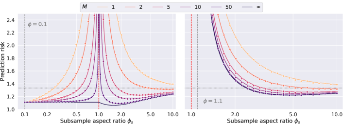
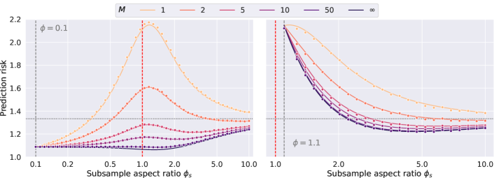
Illustration of Theorem 3.1.
Before we delve into the proof outline for Theorem 3.1, we first provide some numerical illustrations under the AR(1) data model. The covariance matrix of an auto-regressive process of order 1 (AR(1)) is denoted by , where for some parameter . The AR(1) data model is defined as follows:
| (M-AR1-LI) |
where is the eigenvector of associated with the top th eigenvalue . From Grenander and Szegö, (1958, pp. 69-70), the top -th eigenvalue can be written as for some . Under model (M-AR1-LI), the signal strength defined in 3 is , which is the limit of . The (M-AR1-LI) model is thus parameterized by two parameters and satisfies 1-5.
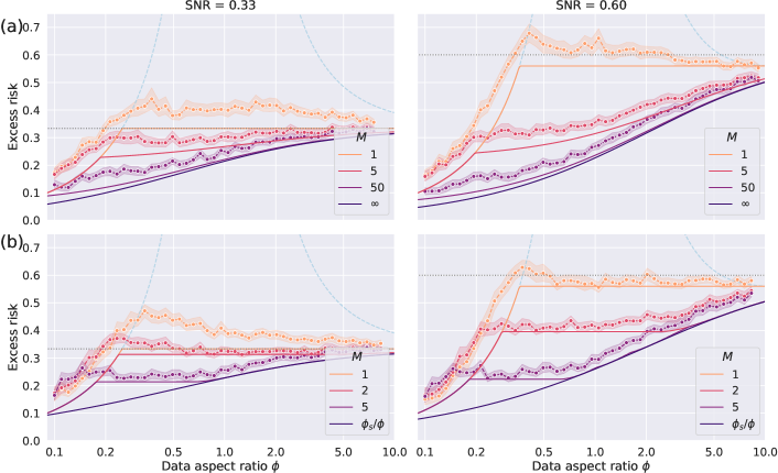
Figures 3 and 4 display the limiting risk for the subagged ridgeless predictor and subagged ridge predictor, respectively, with the number of bags varying from to . In the figures, the limiting aspect ratio of the full data is fixed to be either 0.1 or 1.1, corresponding to the cases when and , respectively. For each case, the limiting aspect ratio of each bag takes values in . We observe that the empirical risks align with the deterministic approximations for both cases, and they are more concentrated around the deterministic approximations as increases. This is expected as the variance of the subagged predictors reduces with . Furthermore, for any fixed , the asymptotic risk decreases as increases.
Due to the non-monotonic risk behavior of the underlying ridge and ridgeless predictors, Figures 3 and 4 show that the best subsample aspect ratio in terms of prediction risk might be strictly larger than . This holds true for any choice of . The case of was already mentioned in Patil et al., 2022b . This observation is intriguing as it suggests it is better to bag predictors that use even fewer observations than the original data. Similar phenomena are also observed in our simulations with varying signal-to-noise ratios; see Patil et al., 2022a (, Appendix S.9.1). We discuss an actionable algorithm for finding the optimal choice of in practice in Section 4.
Proof outline of Theorem 3.1.
The proof of Theorem 3.1 employs the reduction strategy discussed in Section 3. In particular, we apply Theorem 2.9 (subsample conditional for and to subsample and data subsample for any ) to prove the theorem. Below we outline the main steps:
-
1.
The deterministic risk approximation to the subsample conditional risk for can be obtained from the results of Patil et al., 2022b that build on those of Hastie et al., (2022).
-
2.
Under the linear model, to analyze the subsample conditional risk for , we first decompose it as follows:
(26) The first term in the display above is non-random. The asymptotic risk approximation for the second term follows from the asymptotics of the subsample conditional risk for . The challenging part is the analysis of the final cross term , due to the non-trivial dependence implied by the overlap between and . Our strategy to obtain a deterministic approximation for such a term is to write for any univariate function . Here denotes the indices of the overlap, and for are the indices of non-overlapping observations. Observe that conditioning on , and are independent datasets. This conditional independence, coupled with the closed-form expression of the ridge predictor, forms a crucial piece in our argument. To carry out this program, we derive conditional deterministic equivalence results for ridge resolvents. The resulting new results here are collected in Section S.7.3.2.
-
3.
To prove the results for the ridgeless predictor, we essentially take the limit as of the deterministic risk approximation for the ridge predictor with regularization . This process requires appealing to a uniformity argument in . See Appendix S.3 for more details.
3.2.2 Monotonicity of bias and variance in number of bags
Monotonicity in the number of bags for both the data conditional risk and the subsample conditional risk follow from (7). In the classical literature of bagging and subagging, however, it has been of interest to better understand the effect of aggregation on not just the risk, but also on the bias and variance. In this section, we show for the ridge and ridgeless predictors, subagging reduces both the bias and the variance. Monotonicity of the risk proved in Theorem 3.1, does not imply the monotonicity of asymptotic bias and variance components. Fortunately, the risk decomposition derived in Theorem 3.1 demonstrates that both asymptotic bias and variance components are monotonic in , as summarized below.
Proposition 3.5 (Improvement due to subagging).
The monotonicity property in Proposition 3.5 does not immediately follow from the decomposition of and in (21) and (22). All that is implied by (21) and (22) is that and either monotonically increase or decrease in . However, Proposition 3.5 confirms that they are both decreasing in . We establish this by demonstrating that and . Moreover, the proposition explicitly distinguishes the cases of non-increasing and strict decreasing of the bias and variance components.
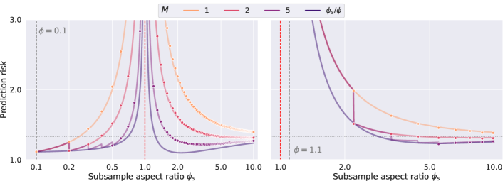
The monotonicity properties claimed in Proposition 3.5 are supported by Figure 5, which shows the bias and variance components for subagged ridgeless predictors under the model (M-AR1-LI). For a similar illustration for subagged ridge predictors, see Patil et al., 2022a (, Figure S.7).
3.3 Splagging without replacement
In this section, we focus on analyzing the risk asymptotics and properties for splagging. More formally, we consider the risk asymptotics of the splagged predictor obtained by averaging the predictors computed on non-overlapping subsets of the data, each of size . This is precisely the splagged predictor . Throughout all the asymptotics below, we consider the permutation to be fixed. Because the limiting risk below does not depend on the permutation , the conclusions continue to hold true even when the data or subsample conditional risk is averaged over all permutations . However, it should be emphasized that this is not the same as the data conditional risk of the splagged predictor averaged over all permutations . In Section 3.3.1, we provide exact risk characterization of splagging without replacement for both ridge and ridgeless predictors. The monotonicity properties of asymptotic bias and variance are then established in Section 3.3.2.
3.3.1 Risk characterization
Recall our convention is defining the splagged predictor as , so that the splagged predictor is well defined for all .
Theorem 3.6 (Risk characterization for splagged ridge and ridgless predictors).
Let be the predictor as defined in (15) for . Suppose Assumptions 1-5 hold for the dataset . Then as , , (and for ), there exist deterministic functions for all , and , such that for ,
Here for , and for , the function decomposes as
| (29) |
where , , , and and are quantities as defined in Theorem 3.1.
Remark 3.7.
For every pair satisfying , note that the splagged predictor and the risks are defined non-trivially only for , and is defined as a constant for . In particular, for a fixed pair , the sequence of risks as changes looks like:
Remark 3.8 (Dependence on data and subsample aspect ratios).
Even though splagging does not formally involve repeated observations like bootstrapping, we will still refer to as the subsample aspect ratio, where is the number of observations in each split part of the full dataset. In Theorem 3.1 for the subagged predictor with replacement, the asymptotic risk depends on both the data aspect ratio as well as the subsample aspect ratio . In contrast, the asymptotic risk for the splagged predictor without replacement in Theorem 3.6 does not depend on the data aspect ratio . This can be seen from the expressions for and . However, it is interesting to note that the asymptotic risk for depends on both and because is finite, which makes the limiting risk of and different. Because defined in (8) is bounded above by 1 and for any , is a strictly better predictor then in terms of the squared risk. In other words, is inadmissible, even asymptotically.
Remark 3.9 (Comparison with distributed learning).
Theorem 3.1 considers the simple average of base predictors fitted on non-overlapped samples, which is also closely related to distributed learning (Mücke et al.,, 2022) that utilizes multiple computing devices to reduce overall training time. Mücke et al., (2022) only provide finite-sample upper bounds for the prediction risk of distributed ridgeless predictor, while Theorem 3.1 gives exact risk characterization. The distributed ridge predictors are also studied in Dobriban and Sheng, (2020), though their goal is to obtain the optimal weight and the optimal regularization parameter.
Illustration of Theorem 3.6.
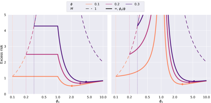
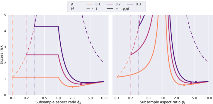
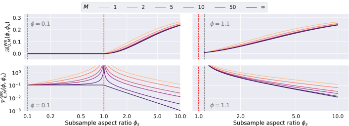
In Figures 6 and 7, we provide numerical illustrations for Theorem 3.6 (bagged ridgeless and ridge predictors with ) under the model (M-AR1-LI), with the number of bags varying from to . The limiting data aspect ratio is fixed at when and at when . We find that the empirical risks align remarkably well with the deterministic approximations, as stated in Theorem 3.6, for both bagged ridge and ridgeless predictors. Mirroring the findings in Figure 3, for any fixed , the optimal may be strictly larger than , an implication of the non-monotonic risk behavior.
Proof outline of Theorem 3.6.
The proof of Theorem 3.6 follows a similar reduction strategy as in the proof of Theorem 3.1, where we first analyze the subsample conditional risks for and , and appeal to Theorem 2.9 to obtain the result for data conditional and subsample conditional risks for any . Below we briefly outline the main steps:
-
1.
The deterministic risk approximation to the subsample conditional risk for splagging is exactly the same as that of subagging.
-
2.
Under the linear model, the subsample conditional risk for decomposes in a similar manner as (26), except in this case, the datasets and are independent of each other (conditional on ), which makes the analysis in this case slightly easier compared to the one for subagging. By conditioning on each of the datasets successively and utilizing the closed-form expression of the ridge estimator, we obtain the desired deterministic approximations.
-
3.
Finally, akin to what we did for Theorem 3.1, we prove results for the ridgeless predictor in the form of the limiting risk approximations to the risk of the ridge predictor in the limit as , based on uniformity arguments.
3.3.2 Monotonicity of bias and variance in number of bags
Just as with subagging, the asymptotic bias and variance components of the conditional risk for splagging are also monotonically decreasing in the number of bags . This is formalized below.
Proposition 3.10 (Improvement due to splagging).
As a concluding remark, because the deterministic risk approximation for splagging is defined as a constant in for , Proposition 3.10 implies that the for every fixed pair , the optimal splagged predictor utilizes bags.
4 Risk profile monotonization
The results presented in the previous sections provide risk characterizations for different variants of bagged predictors, per (2), for all possible subsample aspect ratios . In practice, the choice of is crucial for achieving optimal prediction performance. Following the cross-validation strategy discussed in Patil et al., 2022b , one can apply cross-validation to choose the optimal in order to obtain the best possible prediction performance by subagging or splagging the base predictor across different subsample sizes. In Section 4.1, we first describe the risk monotonization results for general predictors, going back to the general setting in Section 2. In Section 4.2, we then specialize the general risk monotonization results to the bagged ridge and ridgeless predictors. In Section 4.3, we provide a comparison between the best subagged and the best splagged predictors, considering all possible choices of both and , when the base predictor is either ridge or ridgeless.
4.1 Bagged general predictors
Several commonly used prediction procedures, such as min--norm least squares and ridge regression, exhibit a non-monotonic risk behavior as a function of the data aspect ratio . This is referred to in the literature as double/multiple descents (Belkin et al.,, 2019; Hastie et al.,, 2022). The deterministic risk approximation, as a function of the aspect ratio , first increases, reaches a peak, and then decreases. This can be understood in the context of fixed dimension and changing sample size as follows: the risk first decreases as the sample size increases up to a certain threshold, after which it starts increasing with a further increase in sample size. This is a counter-intuitive behavior from a conventional statistical viewpoint, as this indicates that more data may hurt performance. However, from a theoretical perspective, additional information should only lead to improved performance. The underlying issue here lies not in the theory but in the sub-optimality of the prediction procedures when applied as-is on the full data.
There are at least two ways in which one can think of improving a given predictor:
-
1.
Obtain a new predictor whose risk is the greatest monotone minorant of the risk of the given prediction procedure. This can be achieved by computing the predictor on a smaller sample size if necessary. Such a procedure is referred to as the zero-step procedure (with ) in Patil et al., 2022b ; see Algorithm 1 for details. The zero-step procedure does the bare minimum to achieve monotone risk.
-
2.
The zero-step procedure (with ) is not a genuine improvement of the base predictor, as it simply computes the same predictor on a smaller dataset. Building upon the positive effects of subagging or splagging mentioned in previous sections, we can further improve on the zero-step procedure by aggregating over multiple subsets of the data. This was already hinted at and illustrated in Patil et al., 2022b . In this section, we delve deeper into this point.
We note from Theorem 3.1 and Figures 3 and 4 that for each , there are essentially infinitely many risk values possible (one for each pair of subsample aspect ratio and the number of bags ). The zero-step procedure (with ) improves on the base predictor by optimizing over , while keeping fixed. Taking a step further, based on our aforementioned results, we can consider optimizing over and (or just over , while fixing ). In the following, we present an actionable algorithm to achieve the optimum over for any fixed . (It is worth noting that we have already established monotonicity over , and one can always choose to be as large as feasible in practice.) We then present Theorem 4.1, in which we prove that the general cross-validation attains the optimum over (asymptotically). Theorem 4.1 provides theoretical guarantees for the cross-validation procedure for general base predictors, extending the results of Patil et al., 2022b to subagging and splagging.
-
•
For subagging, let denote the subagged predictor as in (2) with bags. Here, represent a simple random sample with or without replacement from the set of all subsets of of size .
-
•
For splagging, is the same as above but now represent a simple random sample without replacement from a random split of into parts with each part containing elements. As explained in Section 3.1, for , no such splitting exists. In this case, we return . Hence in general, we have .
| if CEN=AVG | (32) | |||
| (33) |
| (34) |
Theorem 4.1 (Risk monotonization by cross-validation).
Suppose that as , . Let be the set of subsample sizes defined in Algorithm 1 and be the set of subsets of of size according to the sampling scheme. Suppose that for any , as , and , there exists a deterministic function such that:
-
(i)
For any and a simple random sample from ,
-
(ii)
For any , is proper and lower semi-continuous over , and is continuous on the set .
Let be the cross-validated predictor returned by Algorithm 1 with base predictor . If the estimated risk defined in (32) or (33) is uniformly (in ) close to the subsample conditional risk with probability converging to , then the following conclusions hold. For subagging with or without replacement, or splagging without replacement, for all , we have
where the function is defined as
Furthermore, if for any , is non-decreasing over , then the function is monotonically increasing for every .
Remark 4.2 (Asymptotic risks are different for subagging and splagging.).
Although Theorem 4.1 presents a unified framework for subagging and splagging, the actual limiting risks can be (and in most cases are) different. This discrepancy arises due to the distinct expressions for assumed asymptotic risks in assumption i of Theorem 4.1.
Remark 4.3 (Exact risk characterization of the cross-validated predictor with stronger assumptions).
Note that Theorem 4.1 does not exactly characterize the risk of cross-validated bagged predictor; it only states that the subsample conditional risk of is asymptotically no larger than . Nevertheless, this is an improvement over the results of Patil et al., 2022b , who proved that the subsample conditional risk of is asymptotically no larger than . For the exact risk characterization of , one can make the stronger assumption that as and ,
which can be used to conclude
The result for bagging without replacement can be extended analogously.
Remark 4.4 (Assumption of uniform consistency of the estimated risk).
The assumption of uniform (in ) closeness of the estimated risk to the subsample conditional risk is meant to represent either
In Section 2 of Patil et al., 2022b , the authors have provided several assumptions on the data distribution and the predictors such that this uniform closeness assumption holds true. In Section 4.2, we will apply Theorem 4.1 for bagged linear predictors which are themselves linear predictors. In this specific case, Theorem 2.22 in the aforementioned work shows that uniform closeness holds true under assumptions on the data distribution alone (no matter what linear predictor is, even those that have diverging risks); see Patil et al., 2022b (, Remarks 2.19 and 2.20). We do not further discuss this uniform closeness condition but only remark that Assumptions 1-5 imply the assumptions of Theorem 2.22 with (the median-of-means estimator). With , sub-Gaussian features imply the assumptions of Theorem 2.22.
4.2 Bagged ridge and ridgeless predictors
Theorem 4.1 provides a very general result that describes the risk behavior of cross-validated bagged predictors in general. Following our results in previous sections that verify condition i of Theorem 4.1 for both ridge and ridgeless predictors, we now specialize Theorem 4.1 to these predictors under Assumptions 1-5.
Theorem 4.5 (Risk monotonicity in aspect ratio).
Suppose that the cross-validated predictor is returned by Algorithm 1 with base predictor and bags, and the conditions in Theorem 3.1 (or Theorem 3.6) hold111111The statement as stated holds for in Algorithm 1. For , we need to assume sub-Gaussian features as discussed in Remark 4.4. with being the limiting risk (or ). Then it holds for all ,
| (35) |
Furthermore, is a monotonically increasing function of for every .
In Theorem 4.5, the monotonicity of implies that for every , for the optimal bagged predictor, more data (i.e, increasing ) cannot hurt. In the plot of Figure 8, we observe slight non-monotonicity of the empirical risk profile for . This is because of the small sample size which does not allow for the optimal cross-validated predictor to be the null predictor. One way to not let this happen (in this specific case) is to always include a perfect “null” predictor in the set of predictors tuned with cross-validation in Algorithm 1.
For splagging without replacement, the simulation results are shown in Figure 8(b). As expected, as the limiting aspect ratio increases, the empirical excess risks are nearly monotone increasing and match with theoretical curves. Another pattern we observe in Figure 8 (splagging without replacement) is that the asymptotic risk may not be monotonically decreasing in when is small. This is because the subsample aspect ratio is restricted by the number of bags in that it cannot be below , and the differences in the range of when using different numbers of bags result in the non-monotonicity when is small. While in the overparameterized region when is large enough, the cross-validated risk for bagging without replacement is guaranteed to be monotonically decreasing in . Furthermore, the choice of guarantees that the risk is always optimal compared to any other value of .
4.3 Optimal subagging versus optimal splagging
The cross-validated predictors discussed previously yield asymptotic optimal risks over subsample aspect ratio for every . As a step further, we can obtain the optimal subagging and optimal splagging by jointly optimizing over both and . From the explicit formulas for the limiting risks for each pair of aspect ratios and each , the optimal bagged risks in the two cases can be compared.
Proposition 4.6 (Comparison of the optimal risk of subagging and splagging).
Under Assumptions 3-5, let and be defined as in Theorem 3.1 and Theorem 3.6, respectively. Then for any and , the following holds:
| (36) |
In words, optimal subagging is at least as good as optimal splagging (without replacement) in terms of squared loss for ridge predictors.
For any dataset with fixed aspect ratio , Proposition 4.6 indicates that the optimal risk for bagged predictor across all possible choices of and subsample aspect ratio is always given by subagging. The optimal subagging and optimal splagging risks in Proposition 4.6 can be written as
| (37) |
where the functions and are defined via
| (38) |
The fact that the optimal risks shown in Proposition 4.6 are the same as shown in (37) follows from the fact that the risks are monotonically decreasing in for subagging and that the risk at is the best for splagging without replacement for any pair . The quantities and represent the best possible subsample aspect ratios for subagging and splagging (without replacement) for every data aspect ratio given. (Minimizers of lower semi-continuous functions over compact domains exist, which is true for the functions in (38) from Theorem 4.5.)
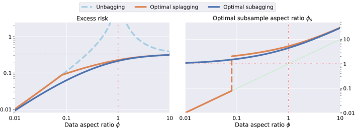
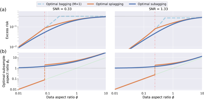
We calculate and present the theoretical optimal asymptotic risks (37) for bagged ridgeless predictors in Figure 9. The optimal risk of the bagged ridgeless predictor with is also presented as the dashed line, which is the same as the monotone risk of the zero-step ridgeless predictor of Patil et al., 2022b with . As shown in Figure 9(a), the optimal risk for the subagged ridgeless predictor is always smaller than the splagged ridgeless predictor without replacement. Both of them improve the risk for the ridgeless predictor with optimal subsample aspect ratio using only one bag ().
Oracle properties of optimal subsample aspect ratios.
From the previous section, we see that optimal subagged ridge or ridgeless regression always outperforms the splagged one in terms of limiting risk. Due to the monotonicity in the number of bags from Proposition 3.5, the optimal risk for subagging must be obtained at for any given subsample aspect ratio . One question that arises is: what is the optimal subsample aspect ratio ? We provide a partial answer to this question in Proposition 4.7 specialized to ridgeless regression.
Proposition 4.7 (Optimal risk for bagged ridgeless predictor).
Suppose the conditions in Theorems 3.1 and 3.6 hold, and are the noise variance and signal strength from Assumptions 2 and 3. Let . For any , the properties of the optimal asymptotic risks and in terms of and are characterized as follows:
-
(1)
: For all , the global minimum of both and are obtained with .
-
(2)
: For all , the global minimum of is obtained at . For , the global minimum of is obtained at ; for , the global minimum of is obtained at .
-
(3)
: If , the global minimum is obtained with any . If , then the global minimums and are obtained at .
Proposition 4.7 implies that the optimal subsample aspect ratio for subagging is always in , i.e., the overparameterized regime. In other words, subagging interpolators with larger aspect ratios (larger than the full data aspect ratio ) helps to reduce the prediction risk, even when . For splagging, however, the minimum risk can be obtained either using the full data or splagging interpolators, depending on the data aspect ratio and the signal-to-noise ratio.
It is interesting to note that the optimal subsampling aspect ratio for splagging is either or it is in the overparameterized regime . This means that either splagging does not help, or when it helps, one has to splag interpolators. Whenever is positive, the optimal subsample aspect ratio is finite for any . Hence we are able to visualize and in Figure 9(b). As shown in Figure 9, there is a point of non-differentiability of for optimal splagging without replacement. Before this point of non-differentiability, , which is the same as the optimal bagged ridgeless with . This is also the same as the ridgeless predictor trained on the full data. After the point of non-differentiability, the optimal risk for splagging without replacement is obtained in the overparameterized regime, i.e., . In contrast to splagging, for all , meaning that it is always better to subag interpolators (i.e., the overparameterized regime).
These observations indicate that, when the number of bags is sufficiently large enough, splagging without replacement only helps when the limiting aspect ratio of the full dataset is above some threshold, but subagging is always beneficial in reducing the prediction risk, even in the underparameterized regime.
Remark 4.8 (Guidelines for practical data analysis).
Proposition 4.7 implies that when using , one should consider bagging interpolators to get better predictive performance, at least when the linear model holds true. However, is practically infeasible particularly when . Note from Figures 3 and 4 that for large enough, the same phenomenon holds true, i.e., it is better to bag interpolators with a large . How large such an should be depends on various unknowns related to the linear model and also on how much gap from one is willing to allow. Given the form of the limiting risk as a function of , we can figure out the necessary value of as a function of the gap , based on the cross-validation procedure (Algorithm 1). Note that this is completely data-driven and model-agnostic. The procedure is as follows: (1) Run Algorithm 1 with and to obtain the estimators and of the limiting subsample conditional risks , respectively, for a grid of values . Following Proposition 2.3, this yields an estimator of the subsample conditional risk for every , in particular, for . (2) Find , the minimizer of . Note that this map is an estimator of the limiting risk for . (3) Fix a tolerance level , and choose
Operating at with such a value of will yield an asymptotic risk that is close (in the additive sense) to the optimal risk.
5 Illustrations and insights
The results discussed so far are derived under Assumptions 1-5 that, in particular, allow for features with arbitrary covariance structure . We will shift our attention to a simpler case of isotropic features (i.e., in Assumption 1). In this case, the spectral distribution simplifies, enabling us to compute the fixed point solutions analytically. Our discussion will primarily revolve around the case of ridgeless predictors for the sake of illustration. While it is possible to obtain similar results for ridge predictors, the resulting expressions would be more involved. In Appendix S.6, we provide formulas for the fixed-point solutions for . From these, one can derive the risk as well as the individual bias and variance numerically for ridge predictors (with arbitrary ). Generally speaking, these quantities can always be computed numerically for nonisotropic models.
In the case of isotropic features, the bias and variance functions presented in Theorems 3.1 and 3.6 take on relatively simple forms, as demonstrated in Corollary 5.1. Furthermore, the asymptotic bias and variance can be computed for all based on (25).
Corollary 5.1 (Bias-variance components for isotropic design).
Assume the conditions in Theorem 3.1 or Theorem 3.6 hold with . Then we have
Subagging with replacement.
Based on Corollary 5.1, we are equipped to evaluate the closed-form asymptotic risk under model (M-ISO-LI):
| (M-ISO-LI) |
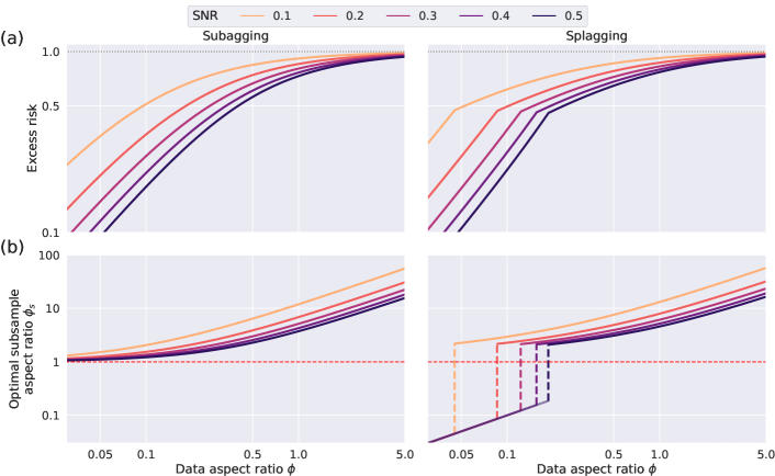
Additional experimental results under model (M-ISO-LI) can be found in Patil et al., 2022a (, Appendix S.9.1). It is worth noting that while the Gaussianity of the noise in model (M-ISO-LI) simplifies numerical evaluation, it is not a requirement for Corollary 5.1. It suffices to have the first and second moments match as above. For , the bias term is always increasing, while the variance term will blow up when the subsample aspect ratio approaches one. However, the variance for is different; it is decreasing in and continuous at . Consequently, one might be interested in the optimal subsample aspect ratio , that best trades off the bias and variance, and minimizes the risk for a given value of and .
Proposition 5.2 (Optimal risk for subagged ridgeless predictors with isotropic features).
Suppose the conditions in Corollary 5.1 hold, and are the noise variance and signal strength from Assumptions 2 and 3. Let . For any , the properties of the asymptotic risk as a function of are characterized as follows:
-
(1)
: The global minimum is obtained at .
-
(2)
: The global minimum
(39) is obtained at where .
-
(3)
: If , then the global minimum is is attained at any . If , then the global minimum is attained at .
As a specific application of Proposition 4.7, Proposition 5.2 provides the analytic expression of the optimal risk attainable through optimization over all choices of the number of bags and the subsample aspect ratio . Additionally, it elucidates the relationship between the optimal risk and the , which is further visualized in Figure 10. Particularly, the optimal subagged risk is monotonically decreasing in when is fixed, which is an intuitive behavior as one would expect a larger results in a smaller prediction risk. In contrast, such a property is not satisfied by the ridge or ridgeless predictor computed on the full data (Hastie et al.,, 2022, Figure 2). It can be shown that the gap between the optimal risk, given in Proposition 5.2, and the underparameterized excess risk , obtained with the full dataset, gets larger when gets smaller. Most importantly, it benefits more when the gets smaller, with a higher overparameterized aspect ratio .
Theorem 5.3 (Optimal subagged ridgeless risk versus optimal ridge risk).
Under the conditions in Corollary 5.1, we have that for all ,
In words, the optimal limiting risk of the subagged ridgeless predictors equals the optimal ridge predictors trained on the full data.
Theorem 5.3 reveals a rather surprising connection between subagging and ridge regression. This result implies that subagging a ridge predictor with and optimizing over the subsample size is “same” as using the ridge predictor with and optimizing over . Consequently, this suggests that subsampling and optimizing over subsample size is a form of regularization. A similar connection between subsampling features and ridge regression was made by LeJeune et al., (2020, Theorem 3.6).
Compared to Theorem 3.6 of LeJeune et al., (2020), our Theorem 5.3 provides the following three key improvements: (1) Subsampling scope. The former theorem focuses solely on the subsampling of features, whereas our theorem considers the sampling of observations. Moreover, in the approach by LeJeune et al., (2020), sampling is restricted to ensure that the final optimal ensemble comprises only least squares estimators. Specifically, they maintain the number of observations in the subsample greater than the number of features, ensuring the existence of a least squares solution for the subsampled data. In contrast, our method permits arbitrary subsample sizes, which means the optimal ensemble can encompass both subsampled least squares and ridgeless interpolators. This distinction is crucial, as there can be scenarios where the optimal subsample might contain more features than observations, a phenomenon highlighted in Proposition 5.2. (2) Signal constraints. The previous theorem limits itself to isotropic random signals . We broaden this scope to incorporate any arbitrary deterministic signals with bounded norms. (3) Distributional assumptions. LeJeune et al., (2020) assumes strong distributional assumptions on the features, noise, and signal, particularly requiring all of them to follow a Gaussian distribution. In comparison, our results do not require such strong distributional assumptions on either the features or the noise and accommodate any deterministic signal with bounded norms.
Remark 5.4 (Difference between optimal subagged ridgeless and optimal ridge predictors).
While Theorem 5.3 suggests that the two optimal limiting risks coincide under the isotropic model, it is important to note the difference in their risk monotonicity properties in the data aspect ratio . The optimal risk of the subagged ridgeless predictor is expected to remain monotonically decreasing in , as shown in Theorem 4.5. In contrast, it is yet to be ascertained whether the optimal ridge predictor has the same property under general models. In the isotropic case, the fixed point parameter can be explicitly solved in terms of the parameters . The explicit formula enables direct analysis of the monotonicity properties of the asymptotic risk and subsequently facilitates the derivation of the optimal risks. However, in the non-isotropic case, such an explicit formula is not available. This lack of an explicit formula calls for a different strategy to extend Theorem 5.3 to non-isotropic features.121212Subsequent to finishing work, Theorem 5.3 has now been extended for non-isotropic cases in Du et al., (2023) by establishing connections between the fixed-point equations involved and utilizing their monotonicity properties.
Splagging without replacement.
Unlike subagging, it is possible, though very cumbersome to obtain the optimal sub-sampling ratio in this case. It involves solving a cubic equation (for a fixed ) or a quartic equation (for the optimal ). Consequently, we resort to numerical computation for and provide a qualitative behavior for next. We observe that as increases, the point of phase transition occurs at a larger value of . This indicates that when there are much more features than samples in the full dataset and the is relatively large, then splagging does not help to reduce the prediction risk. However, when the is small, splagging interpolators is beneficial, even when is much larger than in the full data set.
Subagging versus splagging.
The comparison between subagging and splagging methods shows interesting findings in terms of prediction risks. Next we briefly summarize these findings concerning the similarities and differences between the two types of bagging strategies for ridgeless predictors. From Figure 10, we observe that for any data aspect ratio and any , subagging can help to reduce the risk with a suitable subsample aspect ratio in the overparameterized regime, if we have enough bags. In contrast, splagging may not help when and is large, even if we optimize over all possible numbers of bags and subsample aspect ratios jointly. For the cases when subagging or splagging is beneficial, the maximal gain compared to the predictor computed on the full data increases as the decreases. When the full data aspect ratio is near , both subagging and splagging substantially reduce the prediction risk; see Figures 3, 4, 6 and 7. Most surprisingly, even if the original dataset is heavily underparameterized, overparameterized subagging always helps, as shown in Figure 9(b). For example, recall in Figure 3 when and (which is a favorable case in classical statistics), subagged ridgeless predictors trained on overparameterized subsampled datasets (e.g., with and ) with bags have smaller prediction risk than least squares fitted on the original data.
6 Discussion
In this paper, we provide a generic reduction strategy for characterizing the prediction risk of general bagged predictors (for two bagging strategies of subagging and splagging). As a function of the number of bags , we show that the asymptotic risk of the -bagged predictor under squared error loss can be expressed as , where and represent the asymptotic squared risks of the -bagged predictor with and , respectively. More generally, for a smooth loss function, we show that the risk of the -bagged predictor is sandwiched between similar convex combinations. In addition, we prescribe a generic cross-validation method to tune the subsample size that aims at obtaining the best subagged predictor, which also serves to monotonize the risk profile of any given prediction procedure.
Following this general strategy, along with certain novel derivations from random matrix theory (to analyze conditional resolvents), we obtain explicit risk characterization for bagged ridge and ridgeless predictors. The risk expressions reveal bias and variance monotonicity in the number of bags. Comparing different variants of bagging for ridge and ridgeless predictors, we show that subagging (with optimal subsample size) improves upon the divide-and-conquer or the data-splitting approach of averaging the predictors computed on different non-overlapping splits of data (with optimal split size). This is especially notable in the overparameterized regime, where the latter data-splitting has been recently observed to improve upon the ridgeless predictor computed on the entire data (Mücke et al.,, 2022) under sub-Gaussian features.
Surprisingly, our results show that, under a well-specified linear model, subagging on properly chosen ridgeless interpolators always improves upon the ridgeless predictor trained on the complete data, even when the entire data has more observations than the number of features. Moreover, our generic and model-agnostic cross-validation procedure provably yields the best ridgeless interpolators for subagging. Further specializing to the case of isotropic features, we prove that the optimal subagged predictor has the asymptotic risk that matches the unbagged ridge predictor with optimally-tuned regularization parameter.
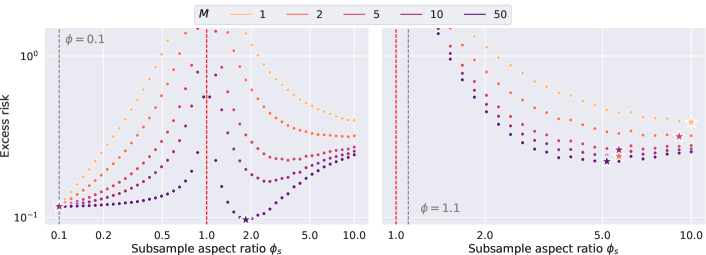
Several natural extensions of the current work can be considered going forward. We briefly discuss two of them below.
First, although our proposed general strategy for analyzing bagged predictors can be helpful for other prediction procedures, we have only derived the precise bagged risk expressions for the ridge and ridgeless regression. In the context of the ridge and ridgeless predictors, we had to develop new random matrix theory tools related to conditional asymptotic equivalents. It may be necessary to develop similar new tools to analyze other predictors based on our strategy. A natural prediction procedure to analyze next for bagging is the lasso or lassoless regression. An empirical investigation of the bagged lassoless predictor has already been conducted by Patil et al., 2022b (see Figure 8, for example). The traditional analysis of this predictor trained on the full data is performed via approximate message passing (AMP) techniques (Li and Wei,, 2021). It would be interesting to see if our general strategy can be combined with AMP, the convex Gaussian min-max theorem, or the leave-one-out perturbation analysis to yield a more encompassing strategy for bagging analysis.
Second, we have analyzed the bagged ridge and ridgeless predictors under a well-specified linear model. It is interesting to extend the analysis to a general data-distributional setting for two main reasons: (1) to make the results more relevant for practical data analysis, and (2) to investigate whether bagging interpolators can still improve upon the ridgeless predictor trained on the full data. Regarding (1) above, the techniques developed by Bartlett et al., (2021) may prove useful in relaxing the linear model assumptions. Regarding (2) above, we performed a simple simulation study that suggests that even in the misspecified nonlinear model, bagging properly selected interpolators can improve the unbagged ridgeless predictor. See Figure 11 for more details. Making these empirical observations more precise presents an exciting avenue for future work.
Acknowledgements
We are indebted to Ryan J. Tibshirani for his constant encouragement and advice throughout this work. We are also indebted to Alessandro Rinaldo, Yuting Wei, Matey Neykov, and other members of the Operational Overparameterized Statistics (OOPS) Working Group at Carnegie Mellon University, for many insightful conversations. We warmly thank the participants of the Theory of Overparameterized Learning Workshop (TOPML) 2022, in particular Daniel LeJeune, for many enlightening discussions.
P. Patil was partially supported by ONR grant N00014-20-1-2787. A. K. Kuchibhotla was partially supported by NSF grant DMS-2113611.
References
- Athey et al., (2019) Athey, S., Tibshirani, J., and Wager, S. (2019). Generalized random forests. The Annals of Statistics, 47(2):1148–1178.
- Bai and Silverstein, (2010) Bai, Z. and Silverstein, J. W. (2010). Spectral Analysis of Large Dimensional Random Matrices. Springer. Second edition.
- Banerjee et al., (2019) Banerjee, M., Durot, C., and Sen, B. (2019). Divide and conquer in nonstandard problems and the super-efficiency phenomenon. The Annals of Statistics, 47(2):720–757.
- Barber et al., (1995) Barber, D., Saad, D., and Sollich, P. (1995). Finite-size effects and optimal test set size in linear perceptrons. Journal of Physics A: Mathematical and General, 28(5):1325.
- Bartlett et al., (2021) Bartlett, P. L., Montanari, A., and Rakhlin, A. (2021). Deep learning: a statistical viewpoint. Acta numerica, 30:87–201.
- Belkin, (2021) Belkin, M. (2021). Fit without fear: remarkable mathematical phenomena of deep learning through the prism of interpolation. Acta Numerica, 30:203–248.
- Belkin et al., (2019) Belkin, M., Hsu, D., Ma, S., and Mandal, S. (2019). Reconciling modern machine-learning practice and the classical bias–variance trade-off. Proceedings of the National Academy of Sciences, 116(32):15849–15854.
- Belkin et al., (2020) Belkin, M., Hsu, D., and Xu, J. (2020). Two models of double descent for weak features. SIAM Journal on Mathematics of Data Science, 2(4):1167–1180.
- Bloemendal et al., (2016) Bloemendal, A., Knowles, A., Yau, H.-T., and Yin, J. (2016). On the principal components of sample covariance matrices. Probability theory and Related Fields, 164(1):459–552.
- Bogachev, (2007) Bogachev, V. I. (2007). Measure Theory. Springer. First edition.
- Breiman, (1996) Breiman, L. (1996). Bagging predictors. Machine Learning, 24(2):123–140.
- Bühlmann and Yu, (2002) Bühlmann, P. and Yu, B. (2002). Analyzing bagging. The Annals of Statistics, 30(4):927–961.
- Buja and Stuetzle, (2006) Buja, A. and Stuetzle, W. (2006). Observations on bagging. Statistica Sinica, pages 323–351.
- Cannings and Samworth, (2017) Cannings, T. I. and Samworth, R. J. (2017). Random-projection ensemble classification. Journal of the Royal Statistical Society: Series B (Statistical Methodology), 79(4):959–1035.
- Chaudhuri, (2014) Chaudhuri, A. (2014). Modern Survey Sampling. CRC Press. First edition.
- Couillet and Debbah, (2011) Couillet, R. and Debbah, M. (2011). Random matrix methods for wireless communications. Cambridge University Press.
- Dar et al., (2021) Dar, Y., Muthukumar, V., and Baraniuk, R. G. (2021). A farewell to the bias-variance tradeoff? An overview of the theory of overparameterized machine learning. arXiv preprint arXiv:2109.02355.
- Deng et al., (2022) Deng, Z., Kammoun, A., and Thrampoulidis, C. (2022). A model of double descent for high-dimensional binary linear classification. Information and Inference: A Journal of the IMA, 11(2):435–495.
- Dereziński, (2023) Dereziński, M. (2023). Algorithmic gaussianization through sketching: Converting data into sub-gaussian random designs. In The Annual Conference on Learning Theory.
- Derezinski et al., (2020) Derezinski, M., Bartan, B., Pilanci, M., and Mahoney, M. W. (2020). Debiasing distributed second order optimization with surrogate sketching and scaled regularization. Advances in Neural Information Processing Systems.
- Dobriban and Sheng, (2020) Dobriban, E. and Sheng, Y. (2020). Wonder: Weighted one-shot distributed ridge regression in high dimensions. Journal of Machine Learning Research, 21(66):1–52.
- Dobriban and Sheng, (2021) Dobriban, E. and Sheng, Y. (2021). Distributed linear regression by averaging. The Annals of Statistics, 49(2):918–943.
- Dobriban and Wager, (2018) Dobriban, E. and Wager, S. (2018). High-dimensional asymptotics of prediction: Ridge regression and classification. The Annals of Statistics, 46(1):247–279.
- Du et al., (2023) Du, J.-H., Patil, P., and Kuchibhotla, A. K. (2023). Subsample ridge ensembles: Equivalences and generalized cross-validation. In International Conference on Machine Learning.
- Duin, (1995) Duin, R. P. W. (1995). Small sample size generalization. In Proceedings of the Scandinavian Conference on Image Analysis, volume 2, pages 957–964. Citeseer.
- Durrett, (2010) Durrett, R. (2010). Probability: Theory and Examples. Cambridge University Press. Fourth edition.
- El Karoui, (2013) El Karoui, N. (2013). Asymptotic behavior of unregularized and ridge-regularized high-dimensional robust regression estimators: rigorous results. arXiv preprint arXiv:1311.2445.
- El Karoui, (2018) El Karoui, N. (2018). On the impact of predictor geometry on the performance on high-dimensional ridge-regularized generalized robust regression estimators. Probability Theory and Related Fields, 170(1):95–175.
- Erdős and Yau, (2017) Erdős, L. and Yau, H.-T. (2017). A Dynamical Approach to Random Matrix Theory. American Mathematical Society.
- Fernández-Delgado et al., (2014) Fernández-Delgado, M., Cernadas, E., Barro, S., and Amorim, D. (2014). Do we need hundreds of classifiers to solve real world classification problems? The Journal of Machine Learning Research, 15(1):3133–3181.
- Friedman and Hall, (2007) Friedman, J. H. and Hall, P. (2007). On bagging and nonlinear estimation. Journal of Statistical Planning and Inference, 137(3):669–683.
- Greene and Wellner, (2017) Greene, E. and Wellner, J. A. (2017). Exponential bounds for the hypergeometric distribution. Bernoulli, 23(3):1911.
- Grenander and Szegö, (1958) Grenander, U. and Szegö, G. (1958). Toeplitz Forms and Their Applications. University of California Press. First edition.
- Gut, (2005) Gut, A. (2005). Probability: A Graduate Course. Springer, New York.
- Hall and Samworth, (2005) Hall, P. and Samworth, R. J. (2005). Properties of bagged nearest neighbour classifiers. Journal of the Royal Statistical Society: Series B (Statistical Methodology), 67(3):363–379.
- Hansen, (1993) Hansen, L. K. (1993). Stochastic linear learning: Exact test and training error averages. Neural Networks, 6(3):393–396.
- Hastie et al., (2022) Hastie, T., Montanari, A., Rosset, S., and Tibshirani, R. J. (2022). Surprises in high-dimensional ridgeless least squares interpolation. The Annals of Statistics, 50(2):949–986.
- Hertz et al., (1989) Hertz, J. A., Krogh, A., and Thorbergsson, G. I. (1989). Phase transitions in simple learning. Journal of Physics A: Mathematical and General, 22(12):2133.
- Hoeffding, (1963) Hoeffding, W. (1963). Probability inequalities for sums of bounded random variables. Journal of the American Statistical Association, pages 13–30.
- Lee, (1990) Lee, A. J. (1990). U-Statistics: Theory and Practice. Routledge. First edition.
- LeJeune et al., (2020) LeJeune, D., Javadi, H., and Baraniuk, R. (2020). The implicit regularization of ordinary least squares ensembles. In International Conference on Artificial Intelligence and Statistics.
- LeJeune et al., (2022) LeJeune, D., Patil, P., Javadi, H., Baraniuk, R. G., and Tibshirani, R. J. (2022). Asymptotics of the sketched pseudoinverse. arXiv preprint arXiv:2211.03751.
- Li and Wei, (2021) Li, Y. and Wei, Y. (2021). Minimum -norm interpolators: Precise asymptotics and multiple descent. arXiv preprint arXiv:2110.09502.
- Liu et al., (2021) Liu, F., Liao, Z., and Suykens, J. (2021). Kernel regression in high dimensions: Refined analysis beyond double descent. In International Conference on Artificial Intelligence and Statistics.
- Loog et al., (2019) Loog, M., Viering, T., and Mey, A. (2019). Minimizers of the empirical risk and risk monotonicity. Advances in Neural Information Processing Systems, 32.
- Loog et al., (2020) Loog, M., Viering, T., Mey, A., Krijthe, J. H., and Tax, D. M. (2020). A brief prehistory of double descent. Proceedings of the National Academy of Sciences, 117(20):10625–10626.
- Lopes et al., (2011) Lopes, M., Jacob, L., and Wainwright, M. J. (2011). A more powerful two-sample test in high dimensions using random projection. Advances in Neural Information Processing Systems.
- Lopes et al., (2018) Lopes, M., Wang, S., and Mahoney, M. (2018). Error estimation for randomized least-squares algorithms via the bootstrap. In International Conference on Machine Learning.
- Mei and Montanari, (2022) Mei, S. and Montanari, A. (2022). The generalization error of random features regression: Precise asymptotics and the double descent curve. Communications on Pure and Applied Mathematics, 75(4):667–766.
- Mhammedi, (2021) Mhammedi, Z. (2021). Risk monotonicity in statistical learning. Advances in Neural Information Processing Systems.
- Miolane and Montanari, (2021) Miolane, L. and Montanari, A. (2021). The distribution of the lasso: Uniform control over sparse balls and adaptive parameter tuning. The Annals of Statistics, 49(4):2313–2335.
- Mücke et al., (2022) Mücke, N., Reiss, E., Rungenhagen, J., and Klein, M. (2022). Data-splitting improves statistical performance in overparameterized regimes. In International Conference on Artificial Intelligence and Statistics, pages 10322–10350. PMLR.
- Muthukumar et al., (2020) Muthukumar, V., Vodrahalli, K., Subramanian, V., and Sahai, A. (2020). Harmless interpolation of noisy data in regression. IEEE Journal on Selected Areas in Information Theory, 1(1):67–83.
- Nakkiran, (2019) Nakkiran, P. (2019). More data can hurt for linear regression: Sample-wise double descent. arXiv preprint arXiv:1912.07242.
- Nakkiran et al., (2021) Nakkiran, P., Venkat, P., Kakade, S. M., and Ma, T. (2021). Optimal regularization can mitigate double descent. In International Conference on Learning Representations.
- Opper, (1995) Opper, M. (1995). Statistical mechanics of learning: Generalization. The handbook of brain theory and neural networks, pages 922–925.
- Opper and Kinzel, (1996) Opper, M. and Kinzel, W. (1996). Statistical mechanics of generalization. In Models of Neural Networks III: Association, Generalization, and Representation, pages 151–209. Springer.
- Opper et al., (1990) Opper, M., Kinzel, W., Kleinz, J., and Nehl, R. (1990). On the ability of the optimal perceptron to generalise. Journal of Physics A: Mathematical and General, 23(11):L581.
- (59) Patil, P., Du, J.-H., and Kuchibhotla, A. K. (2022a). Bagging in overparameterized learning: Risk characterization and risk monotonization. arXiv preprint arXiv:2210.11445.
- (60) Patil, P., Kuchibhotla, A. K., Wei, Y., and Rinaldo, A. (2022b). Mitigating multiple descents: A model-agnostic framework for risk monotonization. arXiv preprint arXiv:2205.12937.
- Patil and LeJeune, (2023) Patil, P. and LeJeune, D. (2023). Asymptotically free sketched ridge ensembles: Risks, cross-validation, and tuning. arXiv preprint arXiv:2310.04357.
- Raudys and Duin, (1998) Raudys, S. and Duin, R. P. W. (1998). Expected classification error of the fisher linear classifier with pseudo-inverse covariance matrix. Pattern recognition letters, 19(5-6):385–392.
- Resnick, (2019) Resnick, S. (2019). A Probability Path. Springer.
- Rosenblatt and Nadler, (2016) Rosenblatt, J. D. and Nadler, B. (2016). On the optimality of averaging in distributed statistical learning. Information and Inference: A Journal of the IMA, 5(4):379–404.
- Rubio and Mestre, (2011) Rubio, F. and Mestre, X. (2011). Spectral convergence for a general class of random matrices. Statistics & probability letters, 81(5):592–602.
- Samworth, (2012) Samworth, R. J. (2012). Optimal weighted nearest neighbour classifiers. The Annals of Statistics, 40(5):2733–2763.
- Sen, (1970) Sen, P. K. (1970). The Hájek-Rényi inequality for sampling from a finite population. Sankhyā: The Indian Journal of Statistics, Series A, pages 181–188.
- Serfling, (1974) Serfling, R. J. (1974). Probability inequalities for the sum in sampling without replacement. The Annals of Statistics, pages 39–48.
- Shiryaev, (2016) Shiryaev, A. N. (2016). Probability-1. Springer. Third edition.
- Srivastava et al., (2016) Srivastava, R., Li, P., and Ruppert, D. (2016). RAPTT: An exact two-sample test in high dimensions using random projections. Journal of Computational and Graphical Statistics, 25(3):954–970.
- Strobl et al., (2009) Strobl, C., Malley, J., and Tutz, G. (2009). An introduction to recursive partitioning: Rationale, application, and characteristics of classification and regression trees, bagging, and random forests. Psychological Methods, 14:323–48.
- Sur et al., (2019) Sur, P., Chen, Y., and Candès, E. J. (2019). The likelihood ratio test in high-dimensional logistic regression is asymptotically a rescaled chi-square. Probability Theory and Related Fields, 175(1):487–558.
- Thrampoulidis et al., (2018) Thrampoulidis, C., Abbasi, E., and Hassibi, B. (2018). Precise error analysis of regularized -estimators in high dimensions. IEEE Transactions on Information Theory, 64(8):5592–5628.
- Thrampoulidis et al., (2015) Thrampoulidis, C., Oymak, S., and Hassibi, B. (2015). Regularized linear regression: A precise analysis of the estimation error. In Conference on Learning Theory, pages 1683–1709. PMLR.
- Vallet et al., (1989) Vallet, F., Cailton, J.-G., and Refregier, P. (1989). Linear and nonlinear extension of the pseudo-inverse solution for learning boolean functions. Europhysics Letters, 9(4):315.
- Viering et al., (2019) Viering, T., Mey, A., and Loog, M. (2019). Open problem: Monotonicity of learning. In Conference on Learning Theory.
- Wang et al., (2017) Wang, S., Gittens, A., and Mahoney, M. W. (2017). Sketched ridge regression: Optimization perspective, statistical perspective, and model averaging. In International Conference on Machine Learning.
- Wu et al., (2021) Wu, Y.-S., Masegosa, A., Lorenzen, S., Igel, C., and Seldin, Y. (2021). Chebyshev-Cantelli PAC-Bayes-Bennett inequality for the weighted majority vote. Advances in Neural Information Processing Systems.
- Zhang et al., (2017) Zhang, C., Bengio, S., Hardt, M., Recht, B., and Vinyals, O. (2017). Understanding deep learning requires rethinking generalization. In International Conference on Learning Representations.
- Zhang et al., (2021) Zhang, C., Bengio, S., Hardt, M., Recht, B., and Vinyals, O. (2021). Understanding deep learning (still) requires rethinking generalization. Communications of the ACM, 64(3):107–115.
Supplement for “Bagging in overparameterized learning:
Risk characterization and risk monotonization”
This document acts as a supplement to the paper “Bagging in overparameterized learning: Risk characterization and risk monotonization.” The section numbers in this supplement begin with the letter “S” and the equation numbers begin with the letter “E” to differentiate them from those appearing in the main paper.
Notation
Below we provide an overview of some general notation used in the main paper and the supplement.
We denote scalars in non-bold lower or upper case (e.g., ), vectors in bold lower case (e.g., ), and matrices in bold upper case (e.g., ). We denote sets using calligraphic letters (e.g., ) and use blackboard letters to denote some special sets: denotes the set of positive integers, denotes the set of real numbers, denotes the set of non-negative real numbers, denotes the set of positive real numbers, denotes the set of complex numbers, denotes the set of complex numbers with positive imaginary part, and denotes the set of complex numbers with negative imaginary part. For a natural number , we use to denote the set .
For a real number , denotes its positive part, its floor, and its ceiling. For a vector , denotes its Euclidean norm. For a pair of vectors and , denotes their inner product. For an event , denotes the associated indicator random variable. For a matrix , denotes its transpose, and denotes its Moore-Penrose inverse. For a square matrix , denotes its trace, and denotes its inverse, provided it is invertible. For a positive semidefinite matrix , denotes its principal square root. A identity matrix is denoted , or simply by when it is clear from the context.
For a real matrix , its operator norm with respect to vector norm is denoted by , and its trace norm is denoted by (recall that ). For a positive semidefinite matrix with eigenvalue decomposition (where is an orthonormal matrix and is a diagonal matrix with non-negative entries), and a function , denotes the positive semidefinite matrix . The notation refers to a diagonal matrix obtained by applying the function to each diagonal entry of .
For symmetric matrices and , denotes the Loewner ordering. For sequences of matrices and , denotes a certain notion of asymptotic equivalence. For more details, see Definitions S.7.2 and S.7.1. We use and to denote probabilistic big-O and little-o notation, respectively. We denote convergence in probability by “”, almost sure convergence by “”, and convergence in distribution by “”.
Organization
Below we outline the structure of the rest of the supplement.
-
•
In Appendix S.0, we collect basic background and results from simple random sampling to analyze bagged predictors.
-
•
In Appendix S.1, we present proofs of results related to general subagged predictors from Section 2.
-
•
In Appendices S.2 and S.3, we present proof of Theorem 3.1 related to subagging from Section 3.2 for ridge and ridgeless predictors, respectively. The proofs for the two cases are separated due to length. However, the proof architecture for the two is similar.
-
•
In Appendix S.4, we present proof of Theorem 3.6 related to splagging from Section 3.3 for ridge and ridgeless predictors. Because some of this proof builds on that of Theorem 3.1, we can combine the two cases of the ridge and ridgeless predictors, unlike the split cases for Theorem 3.1.
-
•
In Appendix S.5, we present proofs of results related to the bias-variance component monotonicity properties in Propositions 3.5 and 3.10 for subagging and splagging, respectively. In this section, we also provide proof of results related to cross-validation and profile monotonicity and those related to oracle properties of optimized bagging from Section 4.
-
•
In Appendix S.6, we present proofs of specialized results related to subagging and splagging under isotopic features from Section 5.
-
•
In Appendix S.7, we formalize several calculus rules for a certain notion of conditional asymptotic equivalence of sequences of matrices that are used in the proofs of constituent lemmas in Appendices S.2, S.3 and S.4.
-
•
In Appendix S.8, we collect various technical helper lemmas related to concentrations and convergences, along with their proofs that are used in proofs in Appendices S.1 to S.4.
-
•
In Appendix S.9, we present additional numerical illustrations for Theorems 3.1, 3.6 and 4.5, and for specialized isotropic results from Section 5.
Appendix S.0 Background on simple random sampling
In Patil et al., 2022b , the authors have proposed a generic algorithm to improve the risk monotonicity behavior of general predictors using strategies analogous to bagging and boosting. Specifically in the context of bagging, they have considered bagged predictors obtained by averaging ingredient predictors trained on subsets of the original data. In that paper, the authors have characterized the risk of the bagged predictor for and crudely bounded the risk of -bagged predictor with that of . However, the numerical simulations presented therein indicate that the -bagged predictor for can perform significantly better than that for , especially around the interpolation threshold. In this paper, our primary goal is to develop tools that can help characterize the risk of the -bagged predictor for any , and also to analyze the corresponding risk monotonization procedure. The -bagged predictor considered in the aforementioned work is obtained by simple random sampling with replacement. In this paper, we also extend our analysis to other versions of bagged predictors to be described shortly. The discussion in this section and that follows (Section 2) pertains to developing different versions of general bagged predictors and their risk characterization.
Because the -bagged predictor is defined through simple random sampling with replacement, the well-known results from survey sampling (Chaudhuri,, 2014) are insightful for understanding its risk behavior. They also provide other versions of the bagged predictors that one can consider. For this reason, we find it helpful to collect and summarize some results from survey sampling about simple random sampling with and without replacement from an appropriate finite population. We briefly mention simple random sampling with replacement (SRSWR) and simple random sampling without replacement (SRSWOR) on an abstract finite population below.
Sampling with replacement.
Suppose we have numbers , a finite population. Let the set of indices be , a finite population. An SRSWR of size from is an i.i.d. draw from with the uniform distribution. An unbiased estimator of the average of elements in the finite population is given by
where is an SRSWR sample of size from . It is very important to stress here that are all fixed numbers, and only are random. Standard results from survey sampling (Chaudhuri,, 2014, Section 2.5) imply that
| (E.1) |
Sampling without replacement.
An SRSWOR of size from is a sample drawn without replacement from , i.e., is drawn from with each element of being equally likely, is drawn from with each element being equally likely, and so on. Define
where are drawn sequentially without replacement from . Once again the only randomness in stems from the randomness of . The results from Chaudhuri, (2014, Section 2.5) imply that
| (E.2) |
Comparing formulas (E.1) and (E.2), one can note that both the averages are unbiased estimators of the mean of elements in the finite population, the variance of SRSWOR estimator is smaller than SRSWR (whenever )131313Note that , if ., and that the variance of SRSWOR estimator becomes zero if . The last fact can be understood by noting that if we draw elements without replacement from a set of elements, we end up with the whole set, and no randomness is left. Note is not well-defined if . This particular restriction of becomes notationally cumbersome in the context of bagging and risk monotonization to be discussed subsequently. To avoid this, we define for . This is natural in the sense that for , when sampling without replacement, there is no randomness left in the estimator . By definition, the variance of the estimator is 0.
Appendix S.1 Proofs in Section 2 (general bagged predictors)
S.1.1 Asymptotic data conditional risk, squared loss
Proof of Proposition 2.2.
The key idea in the proof is to use the conditional risk decomposition from Proposition 2.1. Below we present the proof for sampling from . The proof for sampling from is analogous.
SRSWR.
Since for and , we have
We can thus write and in terms of and as
Substituting in (E.3), we obtain
Thus, subtracting the desired target in (10) for with replacement from both sides, we get
Taking absolute values on both sides and using triangle inequality yields
Taking supremum over , we have
Finally, since we have
the desired claim in (10) for with replacement follows.
SRSWOR.
For SRSWOR from , similarly we have
| (E.4) |
where . Since for and ,
We can thus write and in terms of and as
Substituting in (E.4), we obtain
Thus, subtracting the desired target in (10) for with replacement from both sides, we get
Taking absolute values on both sides and using triangle inequality yields
Taking supremum over , we have
Finally, since we have
the desired claim in (10) for the case of sampling without replacement follows. ∎
S.1.2 Asymptotic subsample conditional risk, squared loss
Before we present the proof for Proposition 2.3, we first show the upper bound of the squared subsample conditional risk for general .
Lemma S.1.1 (Bounding the squared subsample conditional risk).
The subsample conditional prediction risk defined in (5) for the bagged predictor can be bounded as:
| (E.5) |
Proof of Lemma S.1.1.
We start by expanding the squared risk as:
In the expansion above, for equality , we used the fact that .
Now, subtracting the desired limit on both sides yields
This completes the proof of the upper bound.
∎
Next, we present the proof of Proposition 2.3.
Proof of Proposition 2.3.
Lemma 2.8 implies the asymptotics for the data conditional risk. Now, consider the asymptotics for the subsample conditional risk of the bagged predictors. From (E.5) of Lemma S.1.1, it holds that
| (E.6) |
This implies that
The first term on the right hand side converges almost surely to zero by Lemma S.8.6 1. To prove that the second term converges to zero, we start by noting that
is a -statistics based on either an SRSWR or an SRSWOR sample conditional on . Theorem 2 in Section 3.4.2 of Lee, (1990) implies that is a reverse martingale conditional on with respect to some filtration, when we have an SRSWR sample (which is the same as an i.i.d. sample). Lemma 2.1 of Sen, (1970) proves the same result when we have an SRSWOR sample. This, combined with Theorem 3 (maximal inequality for reverse martingales) in Section 3.4.1 of Lee, (1990) (for 141414Theorem 3 of Section 3.4.1 is only stated with , but from the proof, it is clear that is a valid choice. ) yields
The right-hand side we know converges to zero almost surely. To see this, we first write as before the right-hand side as . We know that for all , as (from the given assumption). Also, we know (E.12) and that the right hand side of (E.12) converges in to its probability limit. Hence, Vitali’s theorem (Bogachev,, 2007, Theorem 4.5.4) implies that converges to zero for all as . Therefore, as , for all ,
Because probabilities are bounded by one, dominated convergence theorem implies that
Therefore,
∎
S.1.3 Conditional risk bounds for convex, strongly-convex, and smooth losses
Proof of Proposition 2.6.
We split the proof into two parts, depending on the assumption imposed on the loss function .
Part (1).
For any loss function convex in the second argument, one can trivially obtain
| (E.7) |
Here the last inequality follows from Jensen’s inequality. Because , we get for any ,
On the other hand, we have by Jensen’s inequality
Summarizing, we get that for any ,
One can further obtain the monotonicity property by noting that for any ,
where represents a permutation of Therefore, for any loss function that is convex in the second argument, we get
Because any (non-random) subset of a simple random sample with/without replacement is itself a simple random sample with/without replacement, taking conditional expectation on both sides conditional on yields
This, in particular, implies that for any . This finishes the proof of the first part of the statement.
Part (2).
If we assume that the loss function is strongly convex and differentiable in the second argument, then we can improve the lower bound of Part 1 in terms of . Formally, if is -strongly convex, i.e., is convex in (for every ), then
Applying Proposition 2.1 and taking the expectation conditional on , we obtain
| (E.8) |
S.1.4 From subsample conditional to data conditional risk,
Proof of Lemma 2.8.
Let us first prove the result when sampling with/without replacement from . The proof for would be analogous. Note that where the expectation is taken over a random draw from . We are given that for every . Although not explicitly highlighted, for clarity it is worth reminding that is a sequence implicitly indexed by . Under this condition, let us note that
by Lemma S.8.6 1, since again the conditional risk for converges for any sequences of indices. To be explicit, the underlying triangular array invoked in Lemma S.8.6 (1) is as described follows: For each , recall where . Note that the random quantity is indexed by and . For drawn from , let be the index such that . The convergence then follows from applying Lemma S.8.6 (1) to the triangular array . Hence, we proved that
| (E.10) |
Now, observe that
| (E.11) |
We will now apply Pratt’s lemma (see, e.g., Theorem 5.5 of Gut, (2005) or Chapter 5 Exercise 30 of Resnick, (2019)) to prove almost sure convergence of . Usually, Pratt’s lemma is applied unconditionally, and here we apply it conditional on . For an easier understanding of the proof, let us write in place of in order to make it clear that we are conditioning on . Recall that is independent of the subsamples for any . In this notation, inequality (E.11) becomes
| (E.12) |
Because for every , there exists a set such that and for all , for every . Applying Pratt’s lemma for every , as and using the fact (E.10) as well as the assumption , we get that
Note that . Therefore, we conclude
| (E.13) |
Therefore, (9) applies to yield asymptotics for the data conditional risk uniformly over . ∎
S.1.5 From subsample conditional to data conditional risk, general
Proof of Theorem 2.9.
The proof follows by combining Propositions 2.2 and 2.3, and Lemma 2.8. ∎
Appendix S.2 Proof of Theorem 3.1 (subagging with replacement, ridge predictor)
For defined in Theorem 3.1, we present the proof for ridge and ridgeless predictors in Theorems S.2.1 and S.3.1. For defined in Theorem 3.1, the conclusion still holds since the limits of the proportions of intersection between two SRSWR and SRSWOR draws from are the same from Lemma S.8.3. For proving the asymptotic conditional risks, we will treat as fixed and use to denote the ingredient predictor associated with regularization parameter .
S.2.1 Proof assembly
Before we present the proof, recall the nonnegative constants defined in (16) and (17): is the unique solution to the fixed-point equation
| (E.14) |
and the nonnegative constants , and are defined via the following equations
| (E.15) |
It helps to first slightly rewrite the statement of Theorem 3.1 for as follows. Though it suffices to analyze the case according to Theorem 2.9, below we will do the risk decomposition for general .
Theorem S.2.1 (Risk characterization of subagged ridge predictor).
Proof of Theorem S.2.1.
In what follows, we will prove the results for being a sequence of integers , , . For simplicity, we drop the subscript when it is clear from the context.
For any , let be a sample from , and be a diagonal matrix with if and 0 otherwise. An illustration of these notations for is shown in Figure S.1. The proof will reduce to analyze the individual terms concerning one dataset , or the cross terms concerning and for .
The ingredient estimator takes the form:
Denote by for simplicity. Let for , we have
which yields
Thus, the conditional risk is given by
where the constant term , bias term , and the variance term are given by
| (E.16) | ||||
| (E.17) | ||||
| (E.18) |
Next we analyze the three terms separately for . From Lemmas S.2.2 and S.2.3, we have that , and
Thus, it remains to obtain the deterministic equivalent for the bias term and the trace term . From Lemma S.2.4 and Lemma S.2.5, we have that for all when and for all when , it holds that
as , , and , where the nonnegative constants and are as defined in (E.15). Therefore, we have shown that for all ,
and for all ,
where
and the components are:
The proof for the boundary case when follows from Proposition S.2.6. Then, we have that the function is continuous on .
Finally, the risk expression for general and the uniformity claim over follow from Theorem 2.9. ∎
S.2.2 Component concentrations
In this subsection, we will show that the cross-term converges to zero and the variance term converge to its corresponding trace expectation.
S.2.2.1 Convergence of the cross term
Lemma S.2.2 (Convergence of the cross term).
Proof of Lemma S.2.2.
Note that
We next bound the squared norm
where the last inequality is due to Assumption 4 and the fact that . By Assumption 3, the above quantity is uniformly bounded in . Applying Lemma S.8.4, we thus have that . ∎
S.2.2.2 Convergence of the variance term
Lemma S.2.3 (Convergence of the variance term).
Proof of Lemma S.2.3.
Note that the first term is the same as the variance term for ridge predictor trained on i.i.d. samples . Notice that is independent of , and
Now, we have almost surely as and from Bai and Silverstein, (2010). From Lemma S.8.5, it follows that
Since , we further have ,
| (E.19) |
The second term involves the cross-term . Note that
Because for are uniformly bounded almost surely, again by Lemma S.8.5, it follows that
Since , we have
| (E.20) |
∎
S.2.3 Component deterministic approximations
S.2.3.1 Deterministic approximation of the bias functional
Lemma S.2.4 (Deterministic approximation of the bias functional).
Proof of Lemma S.2.4.
From Lemma S.7.9 (1) we have that for ,
| (E.21) |
By the definition of deterministic equivalent, we have
| (E.22) |
where the last equality holds since and have compact supports and Assumptions 3 and 5.
For the cross term, it suffices to derive the deterministic equivalent of . We begin with analyze the deterministic equivalent of . Let be the number of shared samples between and , we use the decomposition
where and are the common and individual covariance estimators of the two datasets. Let and for . Then
| (E.23) |
where the equalities hold because is invertible when . Conditioning on , we will show a sequence of deterministic equivalents
where in each step, we consider randomness from , , and , respectively, since they are independent of each other conditioning on . The subscript of the deterministic equivalent indicates the dependence on the corresponding random variables, and we will specify each deterministic equivalent in the following proof.
When , we have and the above asymptotic equation reduces to (E.21). We next prove the case when .
Part (a).
Since is independent of conditioning on , from Definition S.7.5 and Lemma S.7.10 (1) we have
where , , , and . Here the subscripts of and are related to the aspect ratio . Because of the sub-multiplicativity of operator norm, we have
By Proposition S.7.6 (2), we have .
Part (b).
Analogously, we have
as .
Part (c).
As we have symmetrized the expression, we have
where . Define . Conditioning on , by Lemma S.7.10 (1), we have
where and . Note that the fixed-point solution depends on . The fixed-point equations reduce to
almost surely. Note that the solution to the above equations is a pair of positive numbers and does not depend on samples. If is a solution to the above system, then is also a solution. Thus, any solution to the above equations must be unique. On the other hand, since satisfies the above equations, it is the unique solution. By Lemma S.7.16, we can replace by the solution of the above system, which does not depend on samples. Thus,
| (E.24) |
where . By Lemma S.7.10 (2), we have
| (E.25) |
where , and and are defined through the following equations:
From Parts (a) to (c), we have shown that for . Note that the above equivalence also holds for . That is, this holds for all . By Proposition S.7.6 (1), we can obtain the unconditioned asymptotic equivalence .
Note that from Lemma S.7.13 and are continuous on , and from Lemma S.8.3, , where is the limiting ratio such that as . We have
where and . Note that
We have
| (E.26) |
is a solution to the first fixed-point equation. From Lemma S.7.12 (2), this solution is also unique. Then, we have
From Lemma S.7.12 (4), we have that . To conclude, we have shown that
| (E.27) |
By the definition of deterministic equivalent, we have
| (E.28) |
where in the last line we used the fact that and have compact supports and Assumptions 3 and 5. The conclusion follows by combining (E.22) and (E.28). ∎
S.2.3.2 Deterministic approximation of the variance functional
Lemma S.2.5 (Deterministic approximation of the variance functional).
Proof of Lemma S.2.5.
From Lemma S.7.9 (2), we have that for ,
| (E.29) |
By the trace rule Lemma S.7.4 (4) , we have
| (E.30) |
where in the last line we used the fact that and have compact supports and Assumption 5.
For the cross term, it suffices to derive the deterministic equivalent of where and . We again show a sequence of deterministic equivalents as in the proof for Lemma S.2.4:
When , this reduces to (E.29). We next show the case when .
Part (a).
We use Lemma S.7.10 (1) to obtain
| (E.31) |
where , , and . Let . Note that conditioning on , almost surely as and from Bai and Silverstein, (2010). Then has bounded operator norm and we have by Proposition S.7.6 (2).
Part (b).
Similarly, we have and .
Part (c).
Note that
where . Define . Conditioning on , by Lemma S.7.10 (1) we have
where and . Note that the fixed-point solution depends on . The fixed-point equations reduce to
almost surely. By the same argument as in the proof for Lemma S.2.4, we have that the solution of the above system does not depend on samples and equals to or almost surely. Thus, by Lemma S.7.16,
where . From Lemma S.7.10 (3), we have
where .
From Parts (a) to (c), we have shown that for . Note that this also holds for . Then by Proposition S.7.6, .
Note that from Lemma S.7.13, and are continuous on , and from Lemma S.8.3, where is the limiting ratio such that as . We have
where , , and . From (E.26), we have that , and
From Lemma S.7.12 (4), we have that . Then we have
| (E.32) |
and thus, we have
| (E.33) |
where in the last line we used the fact that and have compact supports and Assumption 5. ∎
S.2.4 Boundary case: diverging subsample aspect ratio
Proposition S.2.6 (Risk approximation when ).
Proof of Proposition S.2.6.
Note that
Then, by the Cauchy-Schwarz inequality, we have
almost surely as and . Thus, we have the following holds almost surely:
where the last inequality holds eventually almost surely since Assumptions 1-3 imply that the entries of have bounded -th moment, and thus from the strong law of large numbers, is eventually almost surely bounded above by for some constant . Observe that operator norm of the matrix is upper bounded where ’s are the singular values of and is the smallest nonzero singular value. As such that , almost surely (e.g., from results in Bloemendal et al., (2016)) and therefore, almost surely. Thus, we have shown that
or equivalently
From Lemma S.7.13, we have
Thus,
and
Therefore, we have . Thus, is well defined and is right continuous at . ∎
Appendix S.3 Proof of Theorem 3.1 (subagging with replacement, ridgeless predictor)
As done in Appendix S.2, for proving the asymptotic conditional risks, we will treat or as fixed. We will use to denote the ingredient predictor associated with regularization parameter .
S.3.1 Proof assembly
We first explicitly write out the statement of Theorem 3.1 for the ridgeless case of . As in Appendix S.2, we obtain the risk decomposition for general though it suffices to analyze the case according to Theorem 2.9.
For ridgeless predictors () and , the scalar is the unique fixed-point solution to the following equation:
| (E.35) |
and the nonnegative constants and are defined via the following equations:
| (E.36) |
When , the quantities defined in (E.35) and (E.36) are interpreted as , and .
Theorem S.3.1 (Risk characterization of subagged ridgeless predictor).
Let be the ingredient predictor as defined in (15). Suppose Assumptions 1-5 hold for the dataset . Then, as such that and and , there exists a deterministic function , , such that for ,
and
Furthermore, the function decomposes as , where the terms are given by and and the functions and are defined as
where the nonnegative constants and are as defined in (E.36).
Proof of Theorem S.3.1.
We use the same notations as in the proof for Theorem S.2.1 and let for all . Note that
We have
where
| (E.37) | ||||
| (E.38) | ||||
| (E.39) |
Next we analyze the three term separately for . From Lemma S.3.2, we have that . Further, from Lemma S.3.4, Lemma S.3.5, and Lemma S.3.6, for all when and for all when , it holds that
as , , and , where
Here, the components are:
and the nonnegative constants and are as defined in (E.36). The proof for the boundary case when follows from Proposition S.3.7. Then, we have that the function is continuous on and lower-semi continuous on .
Finally, the risk expression for general and the uniformity claim over follow from Theorem 2.9. ∎
S.3.2 Component concentrations
In this subsection, we will show that the cross-term converges to zero and the variance term converge to its corresponding trace expectation.
S.3.2.1 Convergence of the cross term
Lemma S.3.2 (Convergence of the cross term).
Proof of Lemma S.3.2.
Note that
We next bound the norm
where the last inequality is due to Assumption 4 and the fact that . By Assumption 3, is uniformly bounded in . From Bai and Silverstein, (2010), almost surely for . Thus, for some constant almost surely. Applying Lemma S.8.4, we thus have that . ∎
S.3.2.2 Convergence of the variance term
Lemma S.3.3 (Convergence of the variance term).
Proof of Lemma S.2.3.
Note that the term is the same as the variance terms for ridge predictor trained on i.i.d. samples . Notice that is independent of , and
Observe that and almost surely as and from Bai and Silverstein, (2010). We have and for some constant almost surely. From Lemma S.8.5, it follows that
Since , we further have
| (E.40) |
The second term involves the cross term . Note that
because and for are uniformly bounded almost surely. By Lemma S.8.5, it follows that
Since , we have
∎
S.3.3 Component deterministic approximations
S.3.3.1 Deterministic approximation of the bias functional
Lemma S.3.4 (Deterministic approximation of the bias functional).
Proof of Lemma S.3.4.
For the first term, we have that for ,
| (E.41) |
Next we analyze the second term, by considering the following two cases separately for .
(1) . Since the singular values of ’s are almost surely lower bounded away from 0, we have almost surely. Then when and .
(2) . We begin with analyzing the deterministic equivalent of . Recall that is the number of shared samples between and , and and are the common and individual covariance estimators of the two datasets. Also note that from (E.27), we have , where
| (E.42) |
and is as defined in (E.36). Let where . For any matrix with trace norm uniformly bounded by ,
where the second inequality holds because and . Since , it follows from Patil et al., 2022b (, Lemma S.6.14) that, there exists such that the magnitudes of and , and their derivatives with respect to are continuous and bounded by for all . Thus, we get
Similarly, in the same interval the derivatives of and with respect to also have bounded magnitudes for . Therefore, the family of functions
forms an equicontinuous family in over . Thus, the convergence in Part 1 of Lemma S.7.9 is uniform in . We can now use the Moore-Osgood theorem and the continuity property from Lemma S.7.15 to interchange the limits to obtain
where
As , replacing the empirical distribution by limiting distribution yields the desired results. ∎
S.3.3.2 Deterministic approximation of the variance functional
Lemma S.3.5 (Deterministic approximation of the variance functional when ).
Proof of Lemma S.3.5.
For the first term, from Patil et al., 2022b (, Proposition S.3.2) we have that for ,
| (E.43) |
Next we analyze the second term for . It suffices to analyze the case when . From Bai and Silverstein, (2010), we have
Then ’s are invertible almost surely. From Lemma S.7.11, we have that for ,
where and for , defined analogously as in the proof for Theorem S.2.1. Thus, conditional on and , we have
by applying the conditional product rule from Proposition S.7.6. When , let and , we further have
where , the second equality is from Lemma S.7.9 (2) and the fixed point solutions are defined by
When , the above equivalent is also valid, which reduces to the case for as in (E.43). Note that from Lemma S.7.13, and are continuous on , and from Lemma S.8.3, where is the limiting ratio such that as . We have
where and the fixed solutions reduce to
Then, we have
| (E.44) |
Lemma S.3.6 (Deterministic approximation of the variance functional when ).
Proof of Lemma S.3.6.
From (E.43) we have
| (E.45) |
For the second term, it suffices to consider the case when . Let and where . Note that . Note that . From Lemma S.2.3 and Lemma S.2.5, we have that for any fixed ,
as , , and , where is as defined in (E.15). Because of the continuity of and in from Lemma S.7.15, we have that
As , we have that almost surely
where the last inequality is because , and
| (E.46) |
where ’s are the eigenvalues of . Similarly, we have is almost surely bounded. Thus, is almost surely bounded over for some constant . Next we consider the derivative
Note that for , we can bound
where ’s are the eigenvalues of . Similarly, we have that is almost surely bounded for By similar argument as in Lemma S.3.3, the following holds almost surely as ,
That is, is almost surely bounded over .
Since , it follows from Patil et al., 2022b (, Lemma S.6.14) that, there exists such that the magnitudes of and , and their derivatives with respect to are continuous and bounded by for all . Thus, over . Similarly, we have are uniformly bounded over . We can now use the Moore-Osgood theorem and the continuity property from Lemma S.7.15 to interchange the limits to obtain
and the conclusion follows. ∎
S.3.4 Boundary case: diverging subsample aspect ratio
Proposition S.3.7 (Risk approximation when ).
Proof of Proposition S.3.7.
Note that
Then, by the Cauchy-Schwarz inequality, we have
almost surely as and . Thus, we have the following holds almost surely:
where the last inequality holds eventually almost surely since Assumptions 1-3 imply that the entries of have bounded 4-th moment, and thus from the strong law of large numbers, is eventually almost surely bounded above by for some constant . Observe that operator norm of the matrix is upper bounded , where is the smallest nonzero singular value of . As such that , almost surely (e.g., from results in Bloemendal et al., (2016)), and therefore, almost surely. Thus, we have shown that
or equivalently,
From Lemma S.7.14 we have
Thus,
and
Therefore, we have . Thus, is well defined and is right continuous at . ∎
Appendix S.4 Proof of Theorem 3.6 (splagging without replacement, ridge and ridgeless predictors)
Proof of Theorem 3.6.
For , following the proof in Theorem S.2.1, the conditional risk is given by
where , , and are defined as
| (E.48) | ||||
| (E.49) | ||||
where and is a diagonal matrix with diagonal entry being if the th sample is in the sub-sampled dataset and 0 otherwise. Note that for splagging, for all .
We analyze each term separately for . From Lemma S.2.2, we have that . From Lemma S.2.3, we have that
| (E.51) |
since the datasets have no overlaps and the cross term vanishes because for . Then, from (E.22) and (E.30), we have that for ,
| (E.52) | ||||
| (E.53) |
as , , and , where the positive constants , and are as defined in (E.15). For the cross term (), setting in (E.24) yields that
Thus,
| (E.54) |
Combining (E.48)-(E.54), we have shown that , where
and the components are:
with , , and .
From Proposition S.2.6 and Proposition S.3.7, we have that for all and ,
and . Then
Thus, the approximation holds when : .
Finally, the risk expression for general and the uniform statement for all follow from Theorem 2.9. ∎
Appendix S.5 Proofs related to bagged risk properties
S.5.1 Bias-variance monotonicities in the number of bags, subagging with replacement
Proof of Proposition 3.5.
Recall that from the proof for Theorem S.2.1, we have
where the nonnegative constants and are defined in (E.14). Since has positive support, is strictly increasing in , and thus, when , and when . Similarly, when and when . Recall that the definitions of and are a convex combination of and , and and , respectively. The proof for ridgeless predictor follows by setting except for . ∎
S.5.2 Bias-variance monotonicities in the number of bags, splagging without replacement
Proof of Proposition 3.10.
For the variance term, as a linear function of is strictly decreasing in if and is zero if or .
For the bias term, when , since , we have that with equality holds if and only if or , if and only if . Then we have
with equality holds if or . When , with equality holds if and only if , if and only if . The monotonicity of in follows analogously.
As , we further have and for all . ∎
S.5.3 Risk monotonization of general bagged predictors by cross-validation
Proof of Theorem 4.1.
We present the proof for bagging with replacement, and the proof for bagging without replacement follows by restricting the support of to . From Theorem 2.9, we have that for any and simple random samples from or , it holds that
as , , and , where
From Patil et al., 2022b (, Lemma 3.8 and Theorem 3.4), we have that
In Patil et al., 2022b , we have assumed that the risk is bounded away from 0 in order to conclude that the relative error converges to 0. But in Theorem 4.1, we conclude only the positive part of the absolute error converges to 0, for which we do not require the risk to be bounded away from 0.
Since is increasing in for any fixed . For ,
where the first inequality follows because , and the second inequality follows because is increasing in for a fixed . Thus, is a monotonically increasing function in . ∎
S.5.4 Risk monotonization of ridge bagged predictors by cross-validation
Proof of Theorem 4.5.
It suffices to verify the two conditions (i) and (ii) in Theorem 4.1. From Theorem 3.1 and Theorem 3.6, condition (i) holds naturally with being the limiting risk (or ) for fixed . For condition (ii), note that when , is continuous over . When , is continuous over and can takes value infinity when tends to 1 from both sides. Thus, is lower semi-continuous over and continuous on the set .
Following Remark 4.4, the uniform risk closeness condition for holds. Then by Theorem 4.1, we have that
Recall that for any fixed , the function
is increasing in . Then as a function of through (20) and (23) is also increasing in for any fixed . For ,
where the first inequality follows because , and the second inequality follows because is increasing in for a fixed . Thus, is a monotonically increasing function in . ∎
S.5.5 Optimal subagging versus optimal splagging
Proof of Proposition 4.6.
Recall that
From Proposition 3.5, we have that
| (E.55) |
where . From Proposition 3.10, we have that for ,
| (E.56) |
On the other hand,
| (E.57) |
Since is strictly decreasing in from Lemma S.7.13 and has nonnegative support from Assumption 5, we have that is nonnegative and increasing in . Also note that
| (E.58) |
Suppose that , we have
where in the second inequality we use (E.58) and the last inequality is from (E.56). ∎
S.5.6 Optimal bag size for ridgeless predictors
Proof of Proposition 4.7.
The proof of Proposition 4.7 follows by combining results from Lemma S.5.1 and Lemma S.5.2 for subagged and splagged ridgeless predictors, respectively. ∎
Lemma S.5.1 (Optimal risk for subagged ridgeless predictor).
Suppose the conditions in Theorem 3.1 hold, and are the noise variance and signal strength from Assumptions 2 and 3. Let . For any , the properties of the optimal asymptotic risk in terms of and are characterized as follows:
-
(1)
: For all , the global minimum is obtained with .
-
(2)
: For all , the global minimum of is obtained at .
-
(3)
: If , the global minimum is obtained with any . If , then the global minimum is obtained at .
Proof of Lemma S.5.1.
From Theorem 3.1, the limiting risk for bagged ridgeless with is given by
Defined in (E.35)-(E.36), and are continuous functions of , which is strictly decreasing over and satisfies from Lemma S.7.14. Then we have is decreasing in over , is increasing in over , and
Also, and remain constant for from (25). Then to determine the global minimum, it suffices to consider the case when . Next, we consider various cases depending on the value of .
-
•
We first consider the case . We consider further sub-cases depending the value of the pair .
-
1.
When and ,
Note that from Lemma S.7.13 is differentiable in with
being negative over and continuous in , and
by Lemma S.7.14 with defined therein. We have that is continuous over . Since from Lemma S.7.14, we have that
(E.59) (E.60) Since is negative over and , we have
(E.61) Combining (E.59)-(E.61), we have that when is large, approaching zero from above as tends to . On the other hand, since for ,
we have
Thus, there exists such that
- 2.
- 3.
-
1.
-
•
Next consider the case when , i.e., and , since is increasing in and is decreasing in , we have that is decreasing in . Thus, the global minimum is obtained at .
- •
∎
Lemma S.5.2 (Optimal splagged ridgeless).
Suppose the conditions in Theorem 3.6 hold, and are the noise variance and signal strength from Assumptions 2 and 3. Let . For any , the properties of the optimal asymptotic risk in terms of and are characterized as follows:
-
(1)
: For all , the global minimum is obtained with .
-
(2)
: For , there exists global minimum of in . For , the global minimum is in .
-
(3)
: If , the global minimum is obtained with any . If , then the global minimum is obtained at .
Proof of Lemma S.5.2.
From Theorem 3.6, the limiting risk for bagged ridgeless with is given by
Defined in (E.35)-(E.36), and are continuous functions of , which is strictly decreasing over and satisfies from Lemma S.7.14. Then is increasing in over and .
-
•
We first consider the case . We consider further sub-cases depending the value of the pair .
-
1.
When and ,
Define functions and as follows:
(E.62) where is defined in Lemma S.7.14. Then , with increasing in and
Next we study the property of . Simple calculation yields that
From Lemma S.7.14 (4), we have that where is defined in Lemma S.7.14. Analogously, . Then as in the proof of Proposition 4.7, one can verify that
satisfies and by utilizing properties in Lemma S.7.14. Furthermore, as
(E.63) we have that when is large, approaching zero from above as tends to . Thus, the minimum of over is obtained in the open interval .
-
2.
When and , since the term is zero, is increasing in . So the minimum over is obtained at .
-
3.
When , while for all . Since is continuous and finite in , by continuity and (E.63) we have .
-
4.
When , the optimal must be obtained in because of (E.63).
-
1.
-
•
Next consider the case when , i.e., and . Then and . When is increasing in ; when , Therefore, the global minimum is obtained at .
-
•
Finally, consider the case when , i.e. and , . As the term is zero when and positive when , we have that for all when . If , since the risk is continuous over , the global minimum exists. Since the derivative is continuous over and (E.63), the minimizer satisfies .
∎
Appendix S.6 Proofs in Section 5 (isotropic features)
S.6.1 Bagged risk for ridgeless regression
Proof of Corollary 5.1.
From Corollary 5.1, we are able to derive the asymptotic bias and variance for and for ridgeless regression with replacement:
Then the asymptotic bias and variance for general would be convex combinations of the above quantities.
On the other hand, the asymptotic bias and variance for splagging without replacement are given by
S.6.2 Optimal subagged ridgeless regression with replacement
Proof of Proposition 5.2.
For and , we have that
Taking the derivative of the right hand side with respect to
and setting it to zero yields that
| (E.64) |
where . Since , we have is a minimizer and
| (E.65) |
which gives the simplified formula. Note that
| (E.66) |
where for all , the functions and are defined as and , with and
Since , , and are nonngative over , and are also nonnegative. Also noted that
we obtain the upper bound for as follows:
| (E.67) |
with equality obtained if and only if .
Next we analyze the function . Note that is decreasing in , we have that the functions and are nonnegative and monotone increasing in . Hence as the product of nonnegative and monotone increasing functions, is also nonnegative and monotone increasing in . Thus, is monotone increasing in and
where the third equality is due to the L’Hospital’s rule. Note that the risk for is given by , we have that obtained the global minimum of over .
For and , from (E.64) and , we have again is a minimizer.
When , since the bias term is zero and variance term is increasing over and increasing over , we have that when (whenever ),
When , we have . Therefore, for all .
When , the variance term for all . If , then for all . If , then is increasing over . Hence, the conclusions follow. ∎
S.6.3 Comparison between subagged and optimal ridge regression
Proof of Theorem 5.3.
As and , the optimal regularization parameter is given by under the isotopic model (Dobriban and Wager,, 2018). The limiting risk of the optimal ridge regression is given by
which is the same the formula given in Proposition 5.2. Thus, the conclusion follows. ∎
Fixed-point equation details for ridge regression
For isotopic features , . When and , (E.75)-(E.77) reduce to
Solving the first equation for gives
| (E.68) |
Then the asymptotic bias and variance defined in Theorem S.2.1 can be evaluated accordingly.
Appendix S.7 Auxiliary asymptotic equivalency results
S.7.1 Preliminaries
We use the notion of asymptotic equivalence of sequences of random matrices in various proofs. In this section, we provide a basic review of the related definitions and corresponding calculus rules.
Definition S.7.1 (Asymptotic equivalence: deterministic version).
Consider sequences and of (random or deterministic) matrices of growing dimensions. We say that and are equivalent and write if almost surely for any sequence of matrices with bounded trace norm such that .
We emphasize that recent work (Dobriban and Sheng,, 2021; Patil et al., 2022b, ) used the deterministic version of the asymptotic equivalence, implicitly assuming that in the definition is deterministic. However, in this paper we need to investigate the asymptotic equivalence relationship conditional on some other sequences. In that direction, we first extend Definition S.7.1 to allow for random , as in Definition S.7.2.
Definition S.7.2 (Asymptotic equivalence: random version).
Consider sequences and of (random or deterministic) matrices of growing dimensions. We say that and are equivalent and write if almost surely for any sequence of random matrices independent of and , with bounded trace norm such that almost surely.
Even though Definition S.7.1 seems to be more restrictive than Definition S.7.2, they are indeed equivalent as shown in Proposition S.7.3. The latter definition allows for more general definition for “conditional” asymptotic equivalents.
Proposition S.7.3 (Equivalence of and ).
Proof of Proposition S.7.3.
Let and be two sequences of random matrices. Suppose that . We next show that holds. For any sequence of random matrices that is independent of and for all , and has bounded trace norm such that as almost surely. Let denote the event that . Then
Above, equality (a) follows from the law of total expectation. Inequality (b) holds almost surely because and is independent of and . This can be seen as follows. Note that is a function of random variables and . Let where the expectation is taken over the randomness in . Since and are independent and , we have that (see, e.g., Shiryaev, (2016, Chapter 2, Section 7, Equation (16)), or Durrett, (2010, Example 5.1.5))
and from Definition S.7.1, we have almost surely. Thus, we can conclude that .
On the other hand, by definition, directly implies , which completes the proof. ∎
The properties for the two types of deterministic equivalents are summarized in Lemma S.7.4. Though most of the calculus rules are the direct consequences from Dobriban and Wager, (2018); Dobriban and Sheng, (2021), the product rule involving random matrices does not immediately follow from previous work.
Lemma S.7.4 (Calculus of deterministic equivalents).
Let , , and be sequences of random matrices. The calculus of deterministic equivalents ( and ) satisfies the following properties:
-
(1)
Equivalence: The relation is an equivalence relation.
-
(2)
Sum: If and , then .
-
(3)
Product: If has uniformly bounded operator norms such that , is independent of and for , and , then .
-
(4)
Trace: If , then almost surely.
-
(5)
Differentiation: Suppose where the entries of and are analytic functions in and is an open connected subset of . Suppose that for any sequence of deterministic matrices with bounded trace norm we have for every and . Then we have for every , where the derivatives are taken entrywise with respect to .
Proof.
The conclusions for directly follow from Dobriban and Wager, (2018); Dobriban and Sheng, (2021). Then, the proof of property (1), (2), (4), and (5) for follows from Proposition S.7.3. It remains to show that the product rule holds for . Since , we have . Then for any sequence of random matrices that have bounded trace norm and are independent of and , we have
Because and , we have that implies conditioning on . Thus,
and by law of total expectation
which holds for any sequence of random matrices that have bounded trace norm and are independent of and . By definition, we have . ∎
Since the asymptotic equivalent relation is equivalent to , we will just ignore the subscript and use the notation “” for simplicity. The subscript will be specified when needed.
S.7.2 Conditioning and calculus
In this section, we extend the notion of asymptotic equivalence of two sequences of random matrices from Definitions S.7.1 and S.7.2 to incorporate conditioning on another sequence of random matrices.
Definition S.7.5 (Conditional asymptotic equivalence).
Consider sequences , and of (random or deterministic) matrices of growing dimensions. We say that and are equivalent given and write if almost surely conditional on , i.e.,
for any sequence of random matrices independent of and conditional on , with bounded trace norm such that as .
Below we formalize additional calculus rules that hold for conditional asymptotic equivalence Definition S.7.5.
Proposition S.7.6 (Calculus of conditional asymptotic equivalents).
Let , , , and be sequences of random matrices.
-
(1)
Unconditioning: If , then .
-
(2)
Product: If has bounded operator norms such that , is conditional independent of and given for , and , then .
Proof of Proposition S.7.6.
Proofs for the two parts appear below.
Part (1).
For any sequence of deterministic matrices with bounded trace norm, we have
because . By the law of total expectation, we have
Thus, . By Proposition S.7.3, we further have .
Part (2).
For any sequence of random matrices , let and denote the event and , respectively. Because , by definition we have
Because and , we have implies conditioning on . Thus we have
holds for any . This implies that . ∎ Other rules in Lemma S.7.4 also hold for conditional asymptotic equivalents. A direct implication of this is that the deterministic equivalents for resolvents we will derive in Section S.7.3 based on these rules can be naturally generalized to allow for conditional asymptotic equivalents given a common sequence of random matrices that are independent of the source sequence.
S.7.3 Standard ridge resolvents and extensions
In this section, we collect various asymptotic equivalents that are used in the proofs of Lemmas S.2.4 and S.2.5, and Lemmas S.3.4, S.3.5 and S.3.6, which serve to prove Theorem 3.1. These equivalents are also subsequently used in the proof of Theorem 3.6.
S.7.3.1 Standard ridge resolvents
The following lemma supplies an asymptotic equivalent for the standard ridge resolvent. The lemma is adapted from Theorem 1 of Rubio and Mestre, (2011) and Theorem 3 of Dobriban and Sheng, (2021).
Lemma S.7.7 (Asymptotic equivalent for standard ridge resolvent).
Suppose for are i.i.d. random vectors that each multiplicatively decompose such that , where is a random vector consisting of i.i.d. entries for , satisfying , , and for some constants and , and is a positive semidefinite matrix satisfying for some constant that is independent of . Let be the concatenated matrix with for as rows, and let denote the random matrix . Let . Then, for , as such that , the following asymptotic equivalence holds:
| (E.69) |
Here the scalar is defined in terms of another scalar by the equation:
| (E.70) |
where is the unique solution in to the fixed-point equation:
| (E.71) |
It is worth noting that both scalars and implicitly depend on . For the sake of concise notation, this dependence is not always explicitly indicated. Nonetheless, such dependence will be clearly stated when considering certain forthcoming extensions. Please see the remark following Lemma S.7.9 for more discussion.
Observe that can be removed from the statement of Lemma S.7.7 by combining (E.70) and (E.71). For , we then have the following asymptotic equivalence:
Here is the unique solution in to the following fixed-point equation:
The next corollary is a simple consequence of Lemma S.7.7. It supplies an asymptotic equivalent for the regularization scaled ridge resolvent. We assume the regularization parameter is real from here onwards.
Corollary S.7.8 (Asymptotic equivalent for the scaled ridge resolvent).
Assume the setting of Lemma S.7.7. For , the following asymptotic equivalence holds:
Here is the unique solution to the fixed-point equation
| (E.72) |
where is the empirical distribution of the eigenvalues of that supported on .
A side remark: the parameter that appears in Corollary S.7.8 is the companion Stieltjes transform of the spectral distribution of the sample covariance matrix . It is also the Stieltjes transform of the spectral distribution of the gram matrix .
The subsequent lemma utilizes Corollary S.7.8, in conjunction with the calculus of deterministic equivalents as outlined in Lemma S.7.4). It provides deterministic equivalents for resolvents required to derive limiting bias and variance of standard ridge regression. The lemma is adapted from Lemma S.6.10 of Patil et al., 2022b . These equivalents are standard and well-established in the prior literature. For example, the variance resolvent in Lemma S.7.9 can be obtained from results in Dobriban and Sheng, (2021), while the bias resolvent in Lemma S.7.9 can be obtained from results in Hastie et al., (2022).
Lemma S.7.9 (Asymptotic equivalents for ridge resolvents associated with generalized bias and variance).
Suppose for are i.i.d. random vectors with each decomposing multiplicatively into , where is a random vector that contains i.i.d. random variables , , each with , , and for some constants and , and is a positive semidefinite matrix with for some constants and that is independent of . Let be the concatenated random matrix with for as its rows, and define . Let . Then, for , as with , the following asymptotic equivalents hold:
-
(1)
Bias of ridge regression:
(E.73) -
(2)
Variance of ridge regression:
(E.74)
Here is the unique solution to the fixed-point equation:
| (E.75) |
and and are defined through by the following equations:
| (E.76) | ||||
| (E.77) |
where is the empirical distribution of the eigenvalues of that is supported on .
Two remarks on Lemma S.7.9 follow:
-
(a)
The dependency of various scalar parameters appearing in Lemma S.7.9 on the matrix is explicitly highlighted the statement. This is because when we extend the current results later in Lemma S.7.10, these parameters depend on the distributions of eigenvalues of matrices other than . In places where it is clear from context, we will write , , , and to denote , , , and , respectively, for notational simplicity.
-
(b)
Lemmas S.7.7 and S.7.9 assume existence of moments of order for some on the entries of , , mentioned in assumption 2. As done in the proof of Theorem 6 of Hastie et al., (2022) in Appendix A.4 of that paper, this can be relaxed to only requiring the existence of moments of order by a truncation argument. We omit the details.
S.7.3.2 Extended ridge resolvents
The subsequent lemma provides an extension to the asymptotic equivalents presented in Lemma S.7.9. It supplies asymptotic equivalents for Tikhonov resolvents, in which the regularization matrix is substituted by . Here represents an arbitrary positive semidefinite random matrix. While the derivation of extended resolvents in Lemma S.7.10 naturally follows from Lemma S.7.9, we have specifically isolated these extensions. This abstraction facilitates their repeated application in our conditioning arguments, especially in the proofs of Theorems 3.1 and 3.6.
Lemma S.7.10 (Asymptotic equivalents for Tikhonov resolvents).
Suppose the conditions in Lemma S.7.9 holds. Let be any symmetric and positive semidefinite random matrix with uniformly bounded operator norm in that is independent of for all . Let . Then the following asymptotic equivalences hold:
-
(1)
Tikhonov resolvent:
(E.78) -
(2)
Bias of Tikhonov regression:
(E.79) -
(3)
Variance of Tikhonov regression:
(E.80)
where , . Here , and defined by (E.75)-(E.77) simplify to the following:
| (E.81) | ||||
| (E.82) | ||||
| (E.83) |
If , then in (1)-(3) can be replaced by , with the empirical distribution of eigenvalues of being replaced by the limiting distribution .
Proof of Lemma S.7.10.
Proofs for the different parts are separated below.
Part (1).
Note that
| (E.84) |
where , and . Using Lemma S.7.7, we have
| (E.85) |
where is the unique solution to the fixed point equation (E.72) such that
Note that . We can apply the product rule from Lemma S.7.4 (3) and get
Part (2).
From Lemma S.7.9 (1), we have
Part (3).
Similar to Part (2), from Lemma S.7.9 (2), we have
Note that the distribution of ’s eigenvalue has positive support. By the continuity of , , and from Lemma S.7.13 (2), (4) and (3), can by replaced by its limit as . ∎
The following lemma concerns the deterministic equivalents of the precision matrix as the weighted average of two sample covariance matrices of subsamples, when the full sample covariance matrix is invertible almost surely. It is useful when we aim to condition on one of the subsampled covariance matrix, which is used in the proof of Lemma S.3.5.
Lemma S.7.11 (Deterministic equivalent of subsamples in the underparameterized regime).
Suppose the conditions in Lemma S.7.9 holds. Let be the sample covariance matrix computed using observations of , and be the sample covariance matrix computed using the remaining samples. Let and . Suppose that as . Then, we have
Proof of Lemma S.7.11.
We first note that when , the eigenvalues of are bounded away from zero almost surely (Bai and Silverstein,, 2010) and hence the inverse is well defined almost surely as .
The idea for the proof is to consider the perturbed resolvent for . Note that since the matrix is almost surely invertible. Then,
Conditioned on , we have
where the intermediate constants are , , , , and satisfy the fixed-point equation
where in final equality, we used the trace property of the asymptotic equivalence
Now note that
where solves the fixed-point equation
Thus, the fixed-point in can be written as
We note that satisfy the fixed-point equation for (from the fixed-point equation for ). Since is a unique solution, this must be the solution. Letting , we observe that is the solution for the fixed-point equation in . Thus, we also have . ∎
S.7.4 Analytic properties of associated fixed-point equations
In this section, we compile results regarding analytical properties of the fixed-point solution as defined in (E.72).
The subsequent lemma affirms the existence and uniqueness of the solution . It establishes a connection between the properties of the derivatives described in Lemma S.7.12 and the properties of as defined in (E.77). Note the latter equals , where the function is as defined in (E.86)
Lemma S.7.12 (Properties of the solution of the fixed-point equation).
Let and be real numbers. Let be a probability measure supported on . Define the function as follows:
| (E.86) |
Then the following properties hold:
-
(1)
For and , there is a unique such that . The function is positive and strictly decreasing over and negative over , with and .
-
(2)
For and , there is a unique such that . The function is positive and strictly decreasing over and negative over , with and .
-
(3)
For and , is differentiable on and its derivative is strictly increasing over , with and .
-
(4)
For and , is differentiable on and its derivative is strictly increasing over , with and .
Proof of Lemma S.7.12.
We consider different parts separately below.
Part (1).
Observe that
where
Note that is positive and strictly decreasing over with and , while is strictly decreasing over with and . Thus, there is a unique such that , and consequently . Because is positive over , and negative over , is positive strictly decreasing over and negative over , with and .
Part (2).
Note that . Since from (1) and , we have that and .
For , since is positive and strictly decreasing over and negative over , and , we have that there exists such that . The properties of over and follow analogously as in (1).
For , since is continuous, positive and strictly decreasing over , by intermediate value theorem, there exists such that , is positive and strictly decreasing for and negative for , with and .
Part (3).
Since is monotone and continuous, it is differentiable. The derivative at is given by
where
Note that the function is positive and strictly decreasing over with and . On the other hand, the function is strictly decreasing over with and . This follows because for ,
where the first inequality in the chain above follows as the support of is , and the last inequality follows since and , which implies that
Thus, , a product of two positive strictly decreasing functions, is strictly decreasing, and in turn, is strictly increasing. Moreover, and .
Part (4).
The conclusion follows by noting that from (3). ∎
Lemma S.7.13 provides the continuity and limiting behavior of the function for ridge regression (). Lemma S.7.14 does the same for ridgeless regression ().
Lemma S.7.13 (Continuity properties in the aspect ratio for ridge regression).
Let and be real numbers. Let be a probability measure supported on . Consider the function , over , where is the unique solution to the following fixed-point equation:
| (E.87) |
Then the following properties hold:
-
(1)
The range of the function is a subset of .
-
(2)
The function is continuous and strictly decreasing over . Furthermore, , and .
-
(3)
The function , where
is positive and continuous over . Furthermore, , and .
-
(4)
The function , where
is positive and continuous over . Furthermore, .
Proof of Lemma S.7.13.
Proofs for the different parts appear below.
Part (1).
Since has positive support, we have
which implies that .
Part (2).
Rearranging (E.87) yields
From Patil et al., 2022b (, Lemma S.6.13), the function
is strictly increasing and continuous over , , and . It is also positive from (1). Since is positive, strictly increasing and continuous over , we have that the function
is strictly increasing and continuous over . By the continuous inverse theorem, we have is strictly increasing and continuous. Note that . Since is continuous and strictly decreasing in , we have is continuous and strictly decreasing over . Moreover, and .
Part (3).
From (2), is continuous in and
is also continuous in . Thus, the function is continuous. Note that
where the inequality holds because is strictly positive and has positive support. Then we have that and is continuous over . Since , it follows that Similarly, from , and the fact that
it follows that
Part (4).
The continuity of follows from the continuity of and . Note that
From the proof in (3), we have
and thus, . ∎
Lemma S.7.14 (Continuity properties in the aspect ratio for ridgeless regression, adapted from Patil et al., 2022b ).
Let and be real numbers. Let be a probability measure supported on . Consider the function , over , where is the unique solution to the followinn fixed-point equation:
| (E.88) |
Then the following properties hold:
-
(1)
The function is continuous and strictly decreasing over . Furthermore, , and .
-
(2)
The function is strictly increasing over . Furthermore, and .
-
(3)
The function , where
is positive and continuous over . Furthermore, , and .
-
(4)
The function , where
is positive and continuous over . Furthermore, , and .
Lemma S.7.15, adapted from Patil et al., 2022b , confirms the continuity and differentiability of the function on the closed interval for a certain constant , provided . This ensures that is well-defined for , and also implies that related functions are bounded.
Lemma S.7.15 (Differentiability properties in the regularization parameter for , adapted from Patil et al., 2022b ).
Let be real numbers. Let be a probability measure supported on . Let be a real number. Let for some constant . For , let denote the solution to the fixed-point equation
Then, the function is twice differentiable over . Furthermore, over , , , and are bounded.
Lemma S.7.16 (Substitutability of the fixed-point solution).
Let and be a matrix function for matrix and , that is continuous in the first augment with respect to operator norm. If such that is independent of , then .
Proof.
For any matrix whose trace norm is bounded by , conditioning on , we have
Since and is continuous in the first argument with respect to operator norm, we have . Thus,
conditioning on . ∎
The lemma below specializes the solution to the fixed-point equations under the isotopic model.
Lemma S.7.17 (Properties of the fixed-point solution with isotopic features).
Let be a probability measure supported on for . For and , the fixed-point equation
has a closed-form solution given by:
Define and via the follow equations:
As we have the following different cases:
Proof of Lemma S.7.17.
For , we have . For ,
by applying L’Hospital’s rule for indeterminate forms. When , we have
Since and are continuous functions of , we have
and for . For , we apply the L’Hospital’ rule to obtain .
∎
Appendix S.8 Helper concentration results
S.8.1 Size of the intersection of randomly sampled datasets
In this section, we collect various helper results concerned with concentrations and convergences that are used in the proofs of Lemma 2.8, Lemmas S.2.4, S.2.5 and S.3.5.
Below we recall the definition of a hypergeometric random variable, along with its mean and variance. See, e.g., Greene and Wellner, (2017) for more related details.
Definition S.8.1 (Hypergeometric random variable).
A random variable follows the hypergeometric distribution if the probability mass function of is as follows:
The expectation and variance of are given by:
The following lemma provides tail bounds for the number of shared observations in two simple random samples adapted from (Hoeffding,, 1963; Serfling,, 1974). See also Greene and Wellner, (2017).
Lemma S.8.2 (Concentration bounds for the number of shared observations).
For , define . Let , define the random variable to be the number of shared samples, and define accordingly. Then the following statements hold:
-
(1)
follows a binomial distribution, with mean . It holds that for all ,
-
(2)
follows a hypergeometric distribution, with mean . It holds that for all ,
(E.89)
The following lemma characterizes the limiting proportions of shared observations in two simple random samples under proportional asymptotics when both the subsample and full data sizes tend to infinity.
Lemma S.8.3 (Asymptotic proportions of the shared observations).
Consider the setting in Lemma S.8.2. Let and be two sequences of positive integers such that is strictly increasing in , for some constant , and . Then, , and .
Proof.
Proofs for the two parts are split below.
Part (1).
For all ,
Because and , there exists , such that for all , . Thus,
By the Borel–Cantelli lemma, we have
As we further have .
Part (2).
Note that
The conclusion then follows analogously, as in Part 1. ∎
S.8.2 Convergence of random linear and quadratic forms
In this section, we collect helper lemmas on the concentration of linear and quadratic forms of random vectors that are used in the proofs of Lemmas S.2.2, S.2.3, S.3.2 and S.3.3.
The following lemma provides the concentration of a linear form of a random vector with independent components. It follows from a moment bound from Lemma 7.8 of Erdős and Yau, (2017), along with the Borel-Cantelli lemma and is adapted from Lemma S.8.5 of Patil et al., 2022b .
Lemma S.8.4 (Concentration of linear form with independent components).
Let be a sequence of random vector with i.i.d. entries , such that for each i, , , for some and constant . Let be a sequence of random vectors independent of such that almost surely for a constant . Then, almost surely as .
The following lemma provides the concentration of a quadratic form of a random vector with independent components. It follows from a moment bound from Lemma B.26 of Bai and Silverstein, (2010), along with the Borel-Cantelli lemma, and is adapted from Lemma S.8.6 of Patil et al., 2022b .
Lemma S.8.5 (Concentration of quadratic form with independent components).
Let be a sequence of random vector with i.i.d. entries , such that for each i, , , for some and constant . Let be a sequence of random matrix such that almost surely as for some constant . Then, almost surely as .
S.8.3 Convergence of Ces̀aro-type mean and max for triangular array
In this section, we collect a helper lemma on deducing almost sure convergence of a Ces̀aro-type mean from almost sure convergence of the original sequence. It is used in the proof of Proposition 2.3 and Lemma 2.8.
Lemma S.8.6 (Convergence of conditional expectation).
For , suppose is a set of random variables defined over the probability space , with almost surely. If there exists a constant such that for all deterministic sequences , then the following statements hold:
-
(1)
,
-
(2)
.
Proof of Lemma S.8.6.
Proofs for the two parts are split below.
Part (1).
We concatenate the sets for all to form a new sequence
That is, for . See Figure S.2 for an illustration.
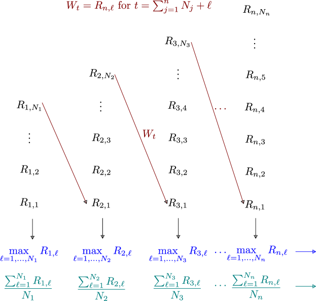
Because if and only if if and only if , it holds that as . Then, by Shiryaev, (2016, Chapter 2, Section 10, Theorem 1), we have that for all ,
Now, for , let be the smallest natural number such that . Since
We further have
or in other words,
Thus, we have that by Shiryaev, (2016, Chapter 2, Section 10, Theorem 1).
Part (2).
We will use the first part. Note that by triangle inequality,
Invoking the first part, we have that .
∎
Appendix S.9 Additional numerical illustrations
S.9.1 Additional illustrations for Theorem 3.1
S.9.1.1 Prediction risk curves for subagged ridgeless and ridge predictors with varying
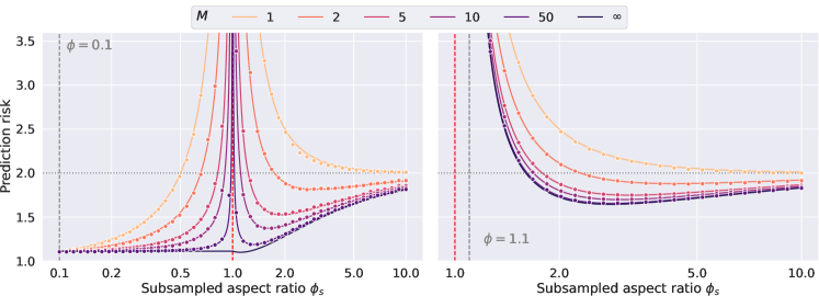
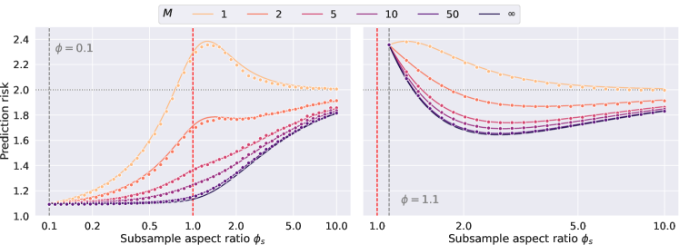
S.9.1.2 Bias-variance curves for subagged ridgeless and ridge predictors with varying
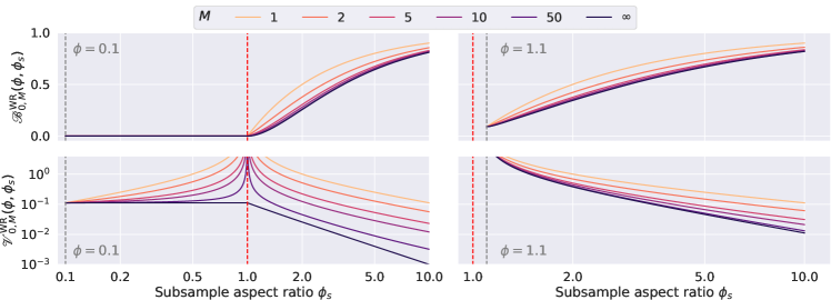
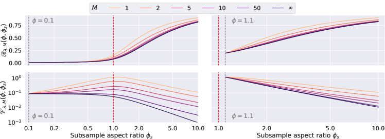
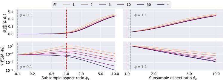
S.9.1.3 Bias-variance curves for subagged ridge predictors with varying ()
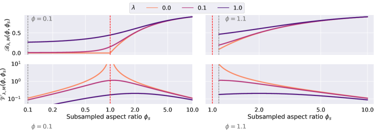
S.9.1.4 Bias-variance curves for subagged ridge predictors with varying ()
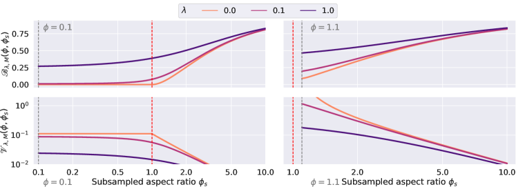
S.9.2 Additional illustrations for Theorem 3.6
S.9.2.1 Prediction risk curves for splagged ridgeless and ridge predictors with varying
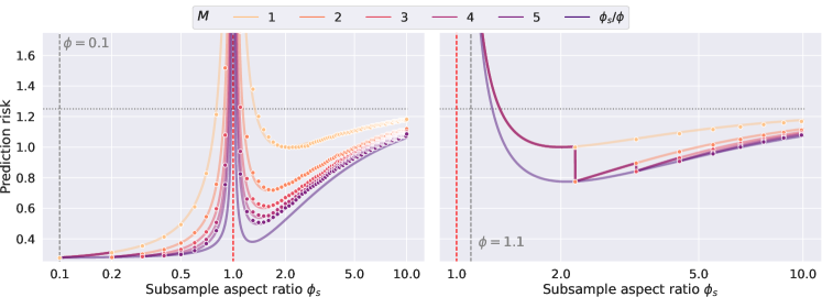
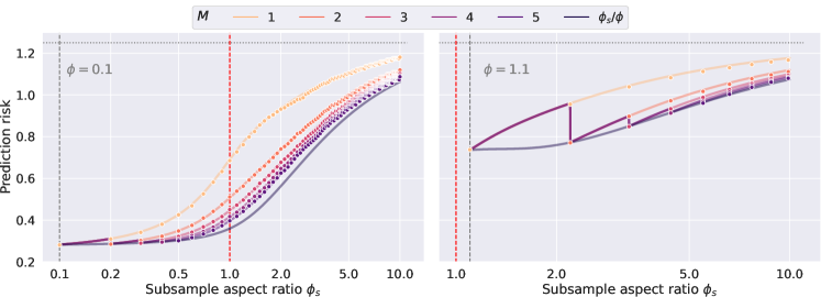
S.9.2.2 Bias-variance curves for ridgeless and ridge predictors with varying

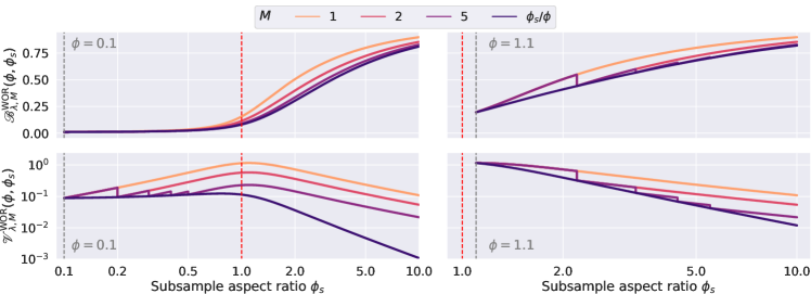
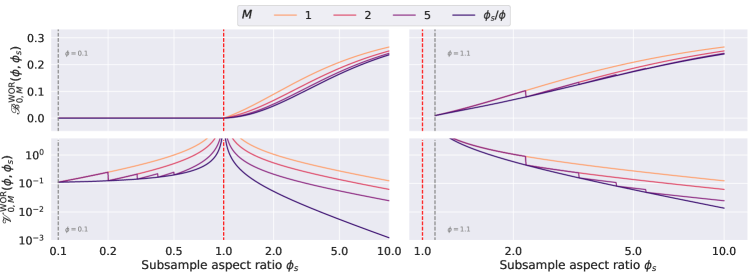

S.9.3 Additional illustrations for Theorem 4.1
S.9.3.1 Risk monotonization for subagged ridgeless and ridge predictors


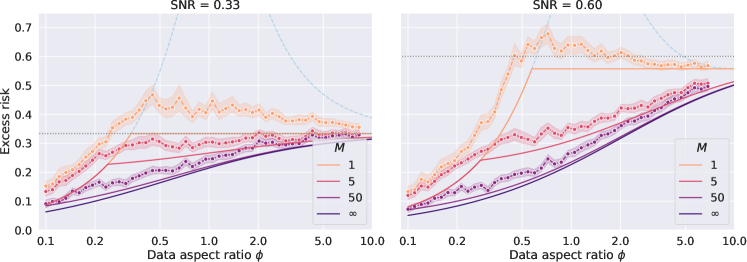
S.9.3.2 Risk monotonization for splagged ridgeless and ridge predictors
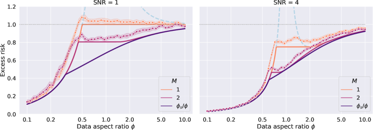
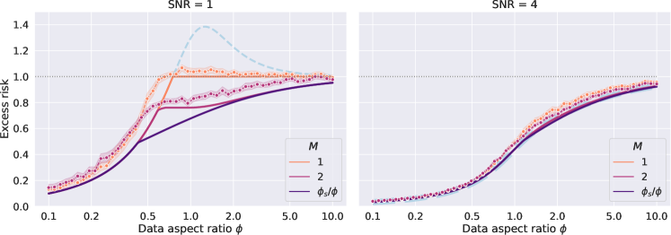
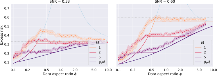
S.9.4 Additional illustrations in Section 5
S.9.4.1 Subagging with replacement and splagging without replacement