How can a Radar Mask its Cognition? ††thanks: Short versions containing partial results appear in the IEEE International Conference on Acoustics, Speech and Signal Processing (ICASSP), 2022, International Conference of Information Fusion (FUSION), 2022 and IEEE International Conference on Decision and Control (CDC), 2022.
Abstract
A cognitive radar is a constrained utility maximizer that adapts its sensing mode in response to a changing environment. If an adversary can estimate the utility function of a cognitive radar, it can determine the radar’s sensing strategy and mitigate the radar performance via electronic countermeasures (ECM). This paper discusses how a cognitive radar can hide its strategy from an adversary that detects cognition. The radar does so by transmitting purposefully designed sub-optimal responses to spoof the adversary’s Neyman-Pearson detector. We provide theoretical guarantees by ensuring the Type-I error probability of the adversary’s detector exceeds a pre-defined level for a specified tolerance on the radar’s performance loss. We illustrate our cognition masking scheme via numerical examples involving waveform adaptation and beam allocation. We show that small purposeful deviations from the optimal strategy of the radar confuse the adversary by significant amounts, thereby masking the radar’s cognition. Our approach uses novel ideas from revealed preference in microeconomics and adversarial inverse reinforcement learning. Our proposed algorithms provide a principled approach for system-level electronic counter-countermeasures (ECCM) to mask the radar’s cognition, i.e. , hide the radar’s strategy from an adversary. We also provide performance bounds for our cognition masking scheme when the adversary has misspecified measurements of the radar’s response.
Index Terms:
Cognitive Radar, Meta-cognition, Revealed Preference, Inverse Reinforcement Learning, Electronic Counter Countermeasures, Bayesian Tracker, Afriat’s TheoremI Introduction
In abstract terms, a cognitive radar is a constrained utility maximizer with multiple sets of utility functions and constraints that allow the radar to deploy different strategies depending on changing environments. Cognitive radars adapt their waveform scheduling and beam allocation by optimizing their utility functions in different situations. If a smart adversary can estimate the utility function or constraints of the cognitive radar, then it can exploit this information to mitigate the radar’s performance (e.g., jam the radar with purposefully designed interference). A natural question is: how can a cognitive radar hide its cognition from an adversary? Put simply, how can a smart sensor hide its strategy by acting dumb? We term this cognition-masking functionality as meta-cognition.111“Meta-cognition” [1] is used to describe a sensing platform that switches between multiple objectives (constrained utility functions). A meta-cognitive radar [1] switches between multiple objectives (plans) to maintain stealth; for example, it can switch between the conflicting objectives of maximizing the signal-to-noise ratio of a target to maximizing privacy of its plan to maintain stealth.
A meta-cognitive radar pays a penalty for stealth - it deliberately transmits sub-optimal responses to keep its strategy hidden from the adversary resulting in performance degradation. This paper investigates how a cognitive radar hide its strategy when the adversary observes the radar’s responses. Our meta-cognition results are inspired by privacy-preserving mechanisms in differential privacy and adversarial obfuscation in deep learning with related works discussed below. Although this paper is radar-centric, we emphasize that the problem formulation and algorithms also apply to adversarial inverse reinforcement learning in general machine learning applications, namely, how to purposefully choose suboptimal actions to hide a strategy.
Related Works
Cognitive radars are widely studied [2, 3]. More recently, our papers [4, 5] deal with inverse reinforcement learning (IRL) algorithms for cognitive radars, namely, how can an adversary estimate the utility function of a cognitive radar by observing its decisions. Reconstructing a decision maker’s utility function by observing its actions is the main focus of IRL [6, 7, 8] in machine learning and revealed preference [9, 10] in micro-economics literature. In the radar literature, such IRL based adversarial actions to mitigate the radar’s operations are called electronic countermeasures (ECM) [11, 12, 4]. This paper builds on [4, 5] and develops electronic counter-countermeasures (ECCM) [13, 14, 15] to mitigate ECM. This paper assumes that adversary’s ECM is unaware if the radar has ECCM capability, which is consistent with state-of-the-art ECCM literature. The central theme of this paper is to apply results from revealed preference in micro-economics theory [9, 16]. To the best of our knowledge, this approach for ECCM to hide cognition is novel.
Several works in literature [17, 18, 19] highlight how an adversary benefits from learning the radar’s utility function. In [17], the adversary optimize its probes to increase the power of its statistical hypothesis test for utility maximization. [18, 19] show how revealed preference-based IRL techniques can be used to manipulate consumer behavior.
In the radar context, [20] uses the Laplacian mechanism for meta-cognition; the cognitive radar anonymizes its trajectories via additive Laplacian noise. In our cognition masking approach, the radar mitigates adversarial IRL via purposeful perturbations from optimal strategy, where the perturbations are computed via stochastic gradient algorithms (see Algorithm 2 in Sec. IV-B).
Context
Radar Design Paradigm: Cognition Masking vs LPI. Low-probability-of-intercept (LPI) radars [21, 22, 23] achieve stealth by minimizing the probability of the radar signals being detected by an adversarial target. Our rationale for stealth in this paper is at a higher level of abstraction than classical LPI. The cognitive radar’s aim is to confuse the adversary’s detector, i.e. , ensure the adversary incorrectly reconstructs the radar’s strategy with high probability.
System level ECCM vs Pulse level ECCM. Our cognition masking algorithm is implemented at the system level (Bayesian tracker level) and not the pulse level (Wiener filter level). Pulse-level ECCM [24, 25, 26] accomplishes LPI-type functionalities for cognitive radars. Cognition masking hides the radar’s strategy from the adversary instead of mitigating the adversary’s detection of the radar’s transmission. Hence, cognition masking ECCM is deployed at a higher level of abstraction than pulse level ECCM.
Hiding Cognition against Optimal IRL vs Sub-optimal IRL. The cognition masking results in this paper assume the adversary performs optimal IRL using Afriat’s theorem [9, 16]. Afriat’s theorem achieves optimal IRL for non-parametric utility estimation of a cognitive radar as it generates a polytope of all viable utilities that rationalizes a finite dataset of adversarial probes and radar responses. However, our cognition masking results can be extended to any potentially sub-optimal IRL algorithm that generates a set-valued estimate of the radar’s utility, as long as the radar has knowledge of the IRL algorithm being used by the adversary. Algorithm 3 in the appendix outlines how a cognitive radar can mask its cognition for an arbitrary IRL algorithm. At an abstract level, cognition masking simply obfuscates a set-valued mapping from the adversary’s dataset to a set of feasible utilities by intelligently distorting the radar’s responses and hence, is not affected by the optimality of adversarial IRL.
At a deeper level, this paper quantifies cognition masking performance when the adversary has misspecified measurements of the radar’s response, and performs sub-optimal IRL. Theorem 8 (in appendix) provides performance guarantees for cognition masking when the radar does not know the misspecification errors and provides a bound on the cognitive masking performance in terms of the error magnitude.
Why not an MDP or non-cooperative game?
In machine learning based IRL [6, 8, 27], the aim is to reconstruct the rewards of a Markov decision process (MDP) subject to entropic constraints on the policy. This requires complete knowledge of the transition dynamics of the adversary’s probes. In comparison, our radar-adversary interaction is batch-wise - the adversary transmits a batch of probe signals, and then the radar responds with a batch of responses. This non-parametric identification of the radar’s strategy is agnostic to transition dynamics in the adversary’s probes. Hence, a static utility maximization setup is more realistic for IRL and inverse IRL involving cognitive radar.
We consider a radar-adversary interaction where the adversary is not aware of the radar’s cognition masking strategy. A more general formulation is a Stackelberg game between the radar and the adversary, with the adversary as the leader and the radar as the follower. However, such an approach for computing the optimal meta-cognition strategy for the radar is ill-posed since the existence of a pure and unique Nash equilibrium is not guaranteed. Finally, from an inverse game theoretic perspective, identifying if the radar-adversary behavior is consistent with Nash equilibrium is intractable since the analyst needs to know both the radar’s and adversary’s utility function. Addressing these issues is beyond the scope of this paper, and the subject of future work.
Outline and Organization of Results
(i) Background. Inverse reinforcement learning (IRL): In Sec. II, we formulate the interaction between a cognitive radar and an adversary target. We review the main idea of revealed preference-based adversarial IRL algorithms, namely, Theorems 1 and 5 used by the adversarial target to reconstruct the radar’s strategy from its actions. Then we outline two examples, namely waveform adaptation and beam allocation. Theorem 6 stated in Appendix -F extends adversarial IRL to the case where the cognitive radar faces multiple constraints. Theorem 6 is omitted from the main text for readability.
(ii) Masking Radar’s Strategy from Adversarial IRL: Sec. III contains our main meta-cognition results, namely, Theorems 2 for mitigating adversarial IRL by masking the radar’s strategy.
The key idea is for the radar to deliberately deviate from its optimal (naive) response to ensure:
(1) its true strategy almost fails to rationalize its perturbed responses (masked from adversarial IRL), and
(2) its performance degradation due to sub-optimal responses does not exceed a particular threshold.
Theorem 7 in Appendix -F extends Theorem 2 to the case where the cognitive radar has multiple constraints. Theorem 8 provides performance bounds on the cognition masking scheme of Theorem 2 when the adversary has misspecified measurements of the radar’s response.
(iii) Masking Radar’s Strategy from Adversarial IRL Detectors in noise.
Sec. IV extends our IRL and cognition masking results to the case where the adversary has noisy measurements of the radar’s response. First, we define IRL detectors (Definition 5) that detect radar’s cognition in noise. Then, we enhance our cognition masking scheme of Theorem 2 to mitigate the IRL detectors. The radar’s cognition masking objective now is to
maximize the detectors’ conditional Type-I error probability, subject to a bound on its deliberate performance degradation.
(iv) Numerical illustration of masking cognition by meta-cognitive radars.
Sec. V illustrates our meta-cognition results on two target tracking functionalities, namely,
waveform adaptation and beam allocation.
Our numerical experiments show that the meta-cognition algorithms in this paper can effectively mask both the radar’s utility function and resource constraint when the cognitive radar is probed by the adversarial target. Our main finding is that a small deliberate performance loss of the meta-cognitive radar suffices to mask the radar’s strategy from the adversary to a large extent.
II Background. IRL to Estimate Cognitive Radar
Since this paper investigates how to construct a cognitive radar that hides its utility from an adversarial IRL system, this section gives the background on how an adversarial system can use IRL to estimate the radar’s utility. An important aspect of the IRL framework below is that it is a necessary and sufficient condition for identifying cognition (utility maximization behavior); hence it can be considered as an optimal IRL scheme. Appendix -H and -G discuss cognition masking when the adversary performs sub-optimal IRL.
II-A Radar-Adversary Dynamics
Definition 1 (Radar-Target Interaction).
The cognitive radar-adversary interaction has the following dynamics:
| (1) |
Remarks. We now give examples for the abstract model (1).
1. A widely used example [28, 29] for the radar-adversary dynamics model (1) is that of linear Gaussian dynamics for target kinematics and linear Gaussian measurements:
| (2) |
Here , . is a block diagonal matrix [30] when the target state represents its position and velocity in Euclidean space. The variables and are mutually independent Gaussian noise processes.
2. In this paper, we are only concerned with the asymptotic statistics of the radar tracker (1) for our cognition-masking algorithms. One example is that of a Bayesian tracker (Kalman filter) where the asymptotic covariance of the state estimate is the unique positive semi-definite solution of the algebraic Riccati equation (ARE). Other tracker examples include the particle filter, interacting multiple model (IMM) filter etc.
We now proceed to define a cognitive radar which we assume in this paper to be a constrained utility maximizer.
Definition 2 (Cognitive Radar).
Remarks.
1. In the main text of this paper, we consider a single constraint. This is consistent with most works in cognitive radar literature which also assume a single operating constraint. For example, in [31], the cognitive radar is constrained by a bound on the target dwell time (monotone in the time the radar spends tracking each target). In [32], the radar’s constraint is a bound on the receiver sensor processing cost (monotone in the radar’s choice of sensor accuracy for target tracking). Hence, we only consider the operating cost of the radar in the main text which is reflected in the radar’s scalar-valued constraint in (3).
2. Multiple resource constraints. Our IRL methodology discussed below can be extended to multiple resource constraints ( is vector-valued). However, for readability, we only consider a scalar-valued constraint in the main text of this paper. We consider multiple resource constraints in Appendix -F. The notation for IRL and cognition masking results is complicated for vector-valued and hence omitted from the main text.
II-B Adversarial IRL for Identifying Strategy of Cognitive Radar
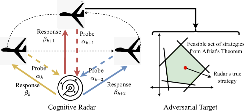
We now review the main results for adversarial IRL, namely, how an adversary can identify and reconstruct the radar’s strategy by observing the radar’s responses. The adversarial IRL system is schematically shown in Fig. 1. The key idea is to formulate the adversary’s task of identifying the radar’s strategy as a linear feasibility problem in terms of the radar’s responses. This paper considers two distinct scenarios in terms of the dependency of the adversary’s probe on the radar’s utility and resource constraint in (3). The two scenarios are formalized in Assumptions 1 and 2 below in our IRL results, Theorems 1 and 5, and justified in Sec. II-C in the tracking examples of waveform adaptation and beam allocation.
IRL for Identifying Utility Function
Theorem 1 below provides a set-valued reconstruction algorithm to estimate the radar’s utility function when the adversary controls the radar’s resource constraint. Such scenarios where the adversary knows the radar’s resource constraint is formalized below in Assumption 1:
Assumption 1.
Theorem 1 (IRL for Identifying Radar’s Utility Function).
Consider the cognitive radar described in Definition 1. Suppose assumption 1 holds. Then:
(a) The adversary checks for the existence of a feasible utility function that satisfies (3) by checking the feasibility of a set of linear inequalities:
| (6) |
where dataset is defined in (5) and the set of inequalities is defined in Appendix -A.
(b) If has a feasible solution, the set-valued IRL estimate of the radar’s utility is given by:
| (7) |
Theorem 1 is well known in micro-economics as Afriat’s theorem [9, 16] and widely used for set-valued estimation of consumer utilities from logged offline data. In complete analogy, the adversary also performs IRL on a batch of probe-response exchanges with the cognitive radar to reconstruct the radar’s utility 222Afriat’s theorem with linear constraints (4) has been generalized to non-linear monotone constraints in literature [33]. For the radar context in this paper, it suffices to assume a linear constraint when the adversary is trying to estimate the radar’s utility. Abstractly, Theorem 1 says that given a finite dataset, the adversary can at best construct a polytope of feasible strategies that rationalize the adversary’s dataset. Theorem 1 achieves IRL when the radar faces a single operating constraint. We discuss adversarial IRL for multiple resource constraints in Theorem 6 in Appendix -F. Then the linear feasibility test of (6) generalizes to a mixed-integer linear feasibility test, linear in the real-valued feasible variables in the multi-constraint case.
IRL for Identifying Radar’s Resource Constraints
In certain scenarios, the utility of the radar is well known (e.g., signal-to-noise ratio), but the operational constraints of the radar are not known. We formalize such scenarios where the adversary knows the radar’s utility function below as Assumption 2:
Assumption 2.
The radar’s utility function (3) is controlled by the adversary’s probe , the radar’s resource constraint is independent of and has the following form:
| (8) |
where are independent of .
IRL objective. The adversary aims to reconstruct using the dataset , where is defined as:
| (9) |
IRL for estimating the radar resource constraints has the same structure as that of Theorem 1 and is discussed in the appendix. IRL for Assumption 2 is formally stated in Theorem 5 in Appendix -B and summarized below:
| (10) | |||
where is the adversary’s set-valued estimate of the radar’s constraint , dataset is defined in (9) and is a feasible vector wrt the feasibility test . Note how the IRL feasibility inequalities in (10) are identical to that of (6) in Theorem 1 but with the inequality direction reversed.
II-C Examples of IRL for Identifying Radar Cognition
Below, we discuss two examples of cognitive radar functionalities, namely, waveform adaptation and beam allocation. Throughout this paper, we will use the two examples below for contextualizing our cognition masking results.
II-C1 Example 1. Waveform Adaptation for Cognitive Radar
Waveform adaptation [34, 35, 36, 37] is a crucial functionality of a cognitive radar. Consider a cognitive radar with linear Gaussian dynamics and measurements (2). The cognitive radar’s aim is to choose the optimal sensor mode (observation noise covariance) based on the target’s maneuvers. A more accurate sensor results in more precise observations, but is also costlier to deploy. Appendix -C formalizes the optimal waveform adaptation and abstracts the problem as the constrained utility maximization problem of (3). The key idea is to assume that adversary’s probe and radar’s response are the eigenvalues of covariance matrices and , respectively, and hence, parameterize the state and observation noise covariance in the state space model of (2). Appendix -C then shows the equivalence between an upper bound on the radar’s asymptotic covariance and the linear constraint . In summary, the cognitive radar’s optimal waveform adaptation strategy can be abstracted as:
| (11) |
where is the radar’s utility, and the linear constraint equivalently bounds the asymptotic precision of the radar.
II-C2 Example 2. Beam allocation for Cognitive Radar
Appendix -D discusses optimal beam allocation [38, 39, 40, 41, 42, 43]. The cognitive radar’s aim is to allocate its beam intensity optimally between multiple targets. Compared to a target with less jerky maneuvers, a target with unpredictable maneuvers requires a more focused beam for the SNR to lie above a certain threshold. Appendix -D formalizes the beam allocation problem and abstracts the problem as a constrained utility maximization problem (3). The key idea is to relate the adversary’s probe to the asymptotic predicted precision of the radar tracker. In summary, the cognitive radar’s optimal waveform adaptation problem can be abstracted as:
| (12) |
where the radar maximizes a Cobb-Douglas utility subject to a bound on the total transmit beam intensity (-norm of intensity vector) for all .
III Inverse IRL. Masking Radar Utility and Constraints from Adversarial IRL
Having discussed how an IRL system can detect a cognitive radar, we are now ready to design a cognitive radar that is aware of the adversary’s IRL motives and hides its strategy (utility function and resource constraints) from the IRL system. In radar terminology, IRL for mitigating a radar system falls under the field of electronic counter measures (ECM). Since meta-cognition deals with spoofing adversarial IRL, it can be viewed as a form of electronic counter-counter measure (ECCM) against ECM.
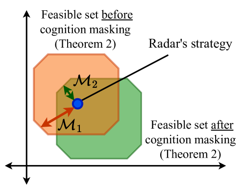
Rationale. How to hide cognition? Recall that the feasibility of (6), (48) is both necessary and sufficient for identifying utility maximization behavior (3); see [9, 16] for the proof. Hence, a cognitive radar’s true strategy lies within the polytope of feasible strategies computed by the adversary (Fig. 1). The cognition masking rationale in this paper is to transmit purposefully designed perturbed responses that ensure the radar’s true strategy lies close to the edge of the polytope of feasible strategies. The distance from the edge of the feasibility polytope is a measure of goodness-of-fit of the strategy to the radar’s responses; see Definitions 3, 4 below. In other words, the radar deliberately sacrifices performance to ensure its strategy poorly rationalizes its perturbed responses, hence hiding its strategy from adversarial IRL.
Main Result. How a radar can mask its utility/constraints
Theorem 2 below is our main result for cognition masking. Theorem 2 uses the concept of feasibility margin - how far is a strategy from failing the IRL feasibility tests (6) or (48). We define two margins - and for the feasibility margins of feasible utilities and constraints , respectively.
Definition 3 (Feasibility Margin for Reconstructed Utility (6)).
Definition 4 (Feasibility Margin for Reconstructed Constraints (48)).
The margin (13), (14) is a measure of goodness-of-fit for the IRL feasibility inequalities (6) and (48), respectively, for any feasible strategy.333 Strictly speaking, the margin (13) is the minimum perturbation so that is infeasible, where is the finite-dimensional projection of for the IRL feasibility test defined in (46) in Appendix -A. However, we abuse notation and express the feasibility test as for the sake of simplicity of exposition. We abuse notation in a similar way for (14) If is a feasible utility that rationalizes (5), we have from (6). Hence, the margin for is the minimum non-negative perturbation so that the IRL test of (6) fails, that is, . Similarly, if is a feasible resource constraint that rationalizes (9), we have from (48). Hence, the margin for is the minimum non-positive perturbation so that the IRL test of (6) fails, that is, . Equivalently, the margin measures how far a strategy lies from the edge of the polytope of feasible strategies. 444There exist several robustness measures in literature [44, 45, 46, 47, 48] that check how well a dataset satisfies economic based rationality. Our cognition masking aim is more subtle - our aim is to ensure a particular strategy rationalizes a dataset poorly by minimizing its feasibility margin (13) (14). The concept of margins arises in many prominent areas of machine learning, for example, in support vector machines (SVM) [49] and also IRL; see [27] for max-margin IRL. In the radar context, a strategy with a large feasible margin is a high-confidence point estimate of the radar’s strategy and hence, at higher risk of getting exposed.
We are now ready to state our first cognition masking result, Theorem 2. Theorem 2 ensures the radar’s true strategy has a low feasibility margin wrt the IRL tests of Theorems 1, 5 by deliberately perturbing the radar’s naive responses (3). In a sense, the radar optimally switches between maximizing its performance and maximizing the privacy of its plan.
Theorem 2 (Masking Cognition from Adversarial IRL Feasibility Tests.).
Consider the cognitive radar (3) from Definition 2. Let denote the naive response sequence (3) that maximizes the cognitive radar’s utility. Then:
(i) Masking Utility Function from IRL.
Suppose Assumption 1 holds. The response sequence defined below masks the radar’s utility from the adversary by ensuring passes the IRL feasibility test (6) with a sufficiently low margin (13) parametrized by :
| (15) | ||||
| (16) |
where dataset is the adversary’s dataset when the radar transmits naive responses , and is defined in (5).
(ii) Masking Resource Constraint from IRL. Suppose Assumption 2 holds.
The response sequence defined below masks the radar’s resource constraint from the adversary by ensuring passes the IRL feasibility test (48) with a sufficiently low margin (14) parametrized by :
| (17) | ||||
| (18) |
where dataset is the adversary’s dataset when the radar transmits naive responses , and is defined in (9).
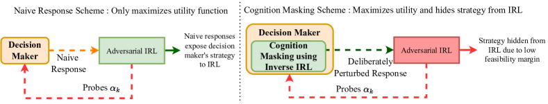
Naive response scheme (Left): The adversary sends a sequence of probe signals to the radar and records its responses to the adversary’s probes. The radar’s strategy passes the IRL feasibility test of Theorem 1 with a large margin if the radar transmits naive responses (3) and can be reconstructed by IRL.
Cognition masking scheme (Right): If the radar is aware of adversarial IRL, the radar deliberately perturbs its responses according to Theorem 2 to hide its strategy from the adversary at the cost of performance degradation. In Sec. V, we illustrate via numerical examples how small deliberate perturbations in the radar’s naive responses mask the radar’s strategy from adversarial IRL to a large extent.
Theorem 2 is our first result for masking cognition; see Algorithm 1 for a step-wise procedure for masking the radar’s utility (15). This is schematically illustrated in Fig. 3. Theorem 2 computes the optimal sub-optimal response of the radar that sufficiently mitigates adversarial IRL. The radar minimizes its performance degradation (maximizes Quality-of-service (QoS)) due to sub-optimal responses, subject to a bound (16), (18) on the feasibility margin of the radar’s strategy (maximizes adversarial confusion). Theorem 2 can be viewed as an inverse IRL (I-IRL) scheme that mitigates an IRL system and is a critical feature of a meta-cognitive radar that switches between different plans. For completeness, Appendix -F extends cognition masking to the case where the cognitive radar faces multiple constraints. Theorem 7 generalizes the cognition masking scheme of Theorem 2 to the multi-constraint case where the adversary uses Theorem 6 for optimal IRL. Also, Appendix -G discusses cognition masking when the adversary has mis-specified measurements of the radar’s responses. Our key result is Theorem 8 that provides a performance bound on the cognition masking scheme of Theorem 2 in terms of the misspecification error magnitude.
Extent of cognition-masking in Theorem 2. A smaller value of implies a larger extent of cognition masking from adversarial IRL and also a greater degradation in the radar’s performance. One extreme case is setting . This results in maximal masking of the radar’s strategy. That is, the IRL feasibility inequalities (6), (48) are no more feasible and there exists no feasible strategy that rationalizes the radar’s responses. Setting also causes the radar to deviate maximally from its naive responses (3), and hence results in a large performance degradation. The other extreme case is setting . In this case, the radar simply transmits its naive response (3) and its strategy is not hidden from the adversary.
Step 1. Compute radar’s naive response sequence by solving the convex optimization problem (3):
where is concave monotone in and is convex monotone in .
Step 2. Choose (extent of cognition masking from IRL feasibility test).
Step 3. Compute upper bound on desired margin (13) after cognition masking:
, where is defined in (13).
Step 4. Compute the cognition-making responses by solving the following optimization problem:
| (19) |
Due to the non-linear margin constraint in (19), the optimization problem can be solved using a general purpose non-linear programming solver, for example, fmincon in MATLAB, to obtain a local minimum.
IV How to Mask Cognition from Detector?
The framework considered in Theorem 2 was deterministic; we assumed that the adversary had accurate measurements of the radar’s responses. In this section, we generalize Theorem 2 to the case where the adversary has noisy measurements of the radar’s decisions. That is, the noise term in the radar’s response measurement in (1) of Definition 1 is a non-zero random variable with pdf . If the adversary deploys a Neyman-Pearson555 By Neyman Pearson’s lemma [50], it is impossible to maximize the Type-I and Type-II error of a detector simultaneously. In this paper, we focus on mitigating the detector by maximizing its conditional Type-I error probability. type detector, how can we design our cognition masking strategy to spoof this detector so that the radar can hide its utility and constraints? Before generalizing Theorem 2 to the noisy case, we first address the following question: How do the adversary’s IRL algorithms, Theorems 1 and 5, adapt to noisy measurements?
IV-A Noisy Adversarial IRL Detectors against Cognitive Radars
Our key IRL results for noisy radar measurements are outlined in Definition 5 below. Recall from Sec. II that the adversary’s IRL algorithm in Theorem 1 comprises a linear feasibility test to identify a feasible strategy that rationalizes the radar’s responses. When the adversary has noisy measurements of the radar’s response, the deterministic feasibility test generalizes to a feasibility hypothesis test to detect the existence of feasible strategies (utilities and constraints) so that the radar responses satisfy utility maximization (3).
For our hypothesis tests below, let and denote the null and alternate hypotheses that the adversary’s noise-less datasets defined in (5) and (9) pass, and not pass, respectively, the IRL feasibility tests (6) and (48), respectively.
| (20) |
The two types of error that arise in hypothesis testing are Type-I and Type-II errors. In the radar context, the Type-I and Type-II errors have the following interpretation:
| (21) |
In analogy to Theorems 1 and 5, our IRL detectors defined below assume two scenarios, namely, Assumptions 3 and 4 that generalize Assumptions 1 and 2, respectively, to the case where the adversary has noisy response measurements.
Assumption 3.
Consider the radar-adversary interaction scenario of Assumption 1. The adversary has access to the noisy dataset defined as:
| (22) |
where is defined in (4), is the radar’s response and is the adversary sensor’s measurement noise (1) with pdf known to the radar.
IRL objective. The adversary uses the IRL detector (25) in Definition 5 to detect if the noise-free dataset (5) passes the IRL test (6) of Theorem 1
Assumption 4.
Consider the radar-adversary interaction scenario of Assumption 2. The adversary has access to the noisy dataset defined as:
| (23) |
where
is the radar’s response, is the adversary sensor’s measurement noise (1) with pdf known to the radar.
IRL objective. The adversary uses the IRL detector (25) in Definition 5 to detect if the noise-free dataset (9) passes the IRL test (48) of Theorem 5
Our IRL hypothesis tests for detecting radar’s cognition (feasible utilities and resource constraints) for noisy radar response measurements are stated in Definition 5 below.
Definition 5 (IRL Detectors for Noisy Response Measurements).
Consider the cognitive radar (3) from Definition 2 and the radar-adversary interaction from Definition 1.
1. IRL for detecting feasible utilities. Suppose Assumption 3 holds.
Then, the statistical test below detects if the radar’s responses satisfy utility maximization behavior (3):
| (24) |
2. IRL for detecting feasible resource constraints. Suppose Assumption 4 holds. Then, the statistical test below detects if the radar’s responses satisfy utility maximization behavior (3):
| (25) |
In the statistical tests (24) and (25):
-
•
is the ‘significance level’ of the test.
-
•
and are random variables defined as:
(26) (27) where is the measurement noise in the adversary’s measurement of the radar’s response (1).
- •
Remarks. 1. The random variable (26) bounds the perturbation needed for to pass the IRL test (6), if holds:
where is the noise-free version of the noisy dataset . Similarly, the random variable (27) bounds the perturbation needed for to pass the IRL test (48), if holds:
where is the noise-free version of the noisy dataset .
2. The IRL detectors (24) and (25) classify the radar as a utility maximizer if the perturbation needed for the feasibility of the IRL inequalities lies under a particular threshold, and vice versa. Consider the statistical test of (24). Eq. 24 can be expressed differently as:
| (30) |
where the RHS term in (30) is the test threshold for test statistic . Intuitively, the larger the perturbation needed for the feasibility of the IRL inequalities, the less confidence the adversary has to classify the radar as a utility maximizer.
Computational Complexity of IRL Detectors. The constrained optimization problems (28) and (29) are non-convex since the RHS of the constraint is bilinear in the feasible variable. However, since the objective function depends only on a scalar, a 1-dim. line search algorithm can be used to solve for in (28) and in (29). That is, for any fixed value of , the constraints in (28), (29) specialize to a set of linear inequalities for which feasibility is straightforward to check.
We now discuss a key feature of the statistical tests (24) and (25) in Theorem 31 that bounds the Type-I error probability of the IRL detectors. Recall that the Type-I error probability is the probability of incorrectly classifying the radar as non-cognitive, when the radar’s response is the solution of a constrained utility maximization problem (3).
Theorem 3 (Performance of IRL Detectors (Definition 5)).
The proof of Theorem 31 is in Appendix -E. The key idea in the proof is to show that, given that the null hypothesis holds, the random variables and dominate the test statistics and , respectively. Since the IRL detectors have a bounded Type-I probability, our cognition masking rationale for the noisy case discussed below is to maximize their conditional Type-I error probability.
IV-B Masking Cognition from IRL Detectors
In the previous section, we generalize the IRL results of Theorem 1 and 5 in Sec. II to the case where the adversary has noisy measurements of the radar’s responses. The key idea is that the IRL feasibility tests (6) and (48) generalize to IRL detectors (24) and (25) in Definition 5, respectively, that detect utility maximization behavior. This section addresses cognition masking when the adversary uses the IRL detectors of Definition 5: How to mitigate the statistical tests of (24) and (25) and make utility maximization detection difficult?
Intuition for hiding cognition from IRL Detectors. Suppose the radar follows the cognition masking scheme of Theorem 2 for the noisy case. Indeed, the radar’s strategy is hidden from the IRL feasibility tests of Theorems 1 and 5, but does not affect the performance of the IRL detectors of Definition 5. To do so, the radar maximizes the conditional Type-I error probability666 The radar can at best maximize the conditional Type-I error probability to mitigate the IRL detectors as the Type-I error probability is bounded by the detectors’ significance level due to Theorem 31. of the IRL detectors by deliberately deviates from its naive responses (3). The conditional Type-I error probability can be viewed as the noisy analog of the inverse of the feasibility margin in the noise-less case.
Definition 6 (Conditional Type-I error probability for IRL Detectors (Definition 5)).
Consider the datasets and defined in (5) and (9), and their corresponding noisy versions and defined in (22) and (23), respectively. Let and denote the minimum perturbations required for the tuples and , respectively, to pass the IRL feasibility tests (6), (48):
| (32) |
where and are the radar’s utility and resource constraint, respectively.
Then:
1. For IRL detector (24), the conditional Type-I error probability, conditioned on (22) and radar’s utility is given by , and defined as:
| (33) |
2. For IRL detector (25), the conditional Type-I error probability conditioned on (23) and radar’s constraint is given by , and defined as:
| (34) |
In (33), (34), the alternate hypothesis event is expressed differently in the equivalent representation form of (30), and the random variables are defined in (26) and (27).
Remarks.
1. The test statistics of the IRL detectors defined in (33) and (34) are computed via an optimization over , whereas the optimization in (34) is over . Hence, and (34) are cheaper to compute than the test statistics (33) and (34), respectively.
2. The IRL detector performance is already constrained due to Theorem 31 (bounded Type-I error probability). Hence, to mitigate the IRL detector, the best the radar can do is to maximize its conditional Type-I error probability using the statistics defined in (32).
We are now ready to state our cognition masking result, Theorem 4, that mitigates IRL detectors (Definition 5). In analogy to Theorem 2 for mitigating the IRL feasibility tests of Theorems 1 and 5, the radar deliberately degrades it performance to maximize the IRL detectors’ conditional Type-I error probability defined in (33) and (34).
Theorem 4 (Masking Cognition from Adversarial IRL Detectors).
Consider the cognitive radar (3) from Definition 2. Let denote the naive response sequence (3) that maximizes the cognitive radar’s utility. Then:
1. Masking Utility Function from Detector. Suppose Assumption 3 holds. Then, the response sequence defined below makes cognition detection difficult by ensuring the detector (24) has a sufficiently large conditional Type-I error probability:
| (35) |
2. Masking Resource Constraint from Detector. Suppose Assumption 4 holds. Then, the response sequence below makes cognition detection difficult by ensuring the detector (25) has a sufficiently large conditional Type-I error probability:
| (36) |
In (35), (36), the positive scalar parametrizes the extent of mitigation of the IRL detector.
Theorem 4 is our second result for cognition masking; see Algorithm 2 for a step-wise procedure for masking cognition in noise (35) when the adversary knows the radar’s constraints. Eq. 35 and 36 compute the optimal sub-optimal radar response that sufficiently hides the radar’s cognition from being detected by the IRL hypothesis tests of Definition 5. The parameter in Theorem 4 is analogous to parameter in Theorem 2. A larger value of (35) results in a larger conditional Type-I error probability for the IRL detector (larger adversarial confusion) while increasing the radar’s deviation from its optimal response (greater performance degradation), and vice versa.
The optimization problems (35) and (36) can be solved by stochastic gradient algorithms. Algorithm 2 outlines a constrained SPSA [51, 52] implementation for computing the cognition masking scheme of Theorem 4. The objective function is non-convex in the radar’s responses, hence SPSA converges to a local optimum. SPSA is a generalization of adaptive algorithms where the gradient computation in (35) requires only two empirical estimates of the objective function per iteration, i.e. , the number of evaluations is independent of the dimension of the radar’s response. For decreasing step size (40), the SPSA algorithm converges with probability one to a local stationary point. For constant step size , it converges weakly (in probability).
Summary: In this section, we generalized our cognition masking results of Theorem 2 to the case where the adversary has noisy measurements of the radar’s responses. We first generalized our adversarial IRL feasibility tests of Theorems 1, 5 to IRL hypothesis tests (24) and (25) in Definition 5 to detect utility maximization behavior given noisy radar response measurements. We then present Theorem 4 that masks the radar’s cognition by making utility maximization detection erroneous by maximizing the conditional Type-I error probability of the IRL detectors via purposeful sub-optimal responses. Our cognition masking results can be extended WLOG to any sub-optimal IRL algorithm and discussed in Appendix -H.
V Numerical Results for I-IRL
In this section, we illustrate how our cognition masking results of Theorems 2 and 4 successfully confuse adversarial IRL via the two radar tracking functionalities, namely, waveform adaptation and beam allocation discussed in Sec. II.
V-A Cognition Masking via Theorem 2 for Noise-less Adversary Measurements
Consider the scenario where the adversary has accurate measurements of the radar’s responses. Recall from Sec. II-C that the adversary knows the radar’s constraints for waveform adaptation and the radar’s utility function for beam allocation. For waveform adaptation, the probe signal parametrizes the state covariance matrix of the radar’s Kalman filter due to the adversary’s maneuvers, and the response signal parametrizes the sensory accuracy chosen by the radar. Recall that the probe signal is the diagonal of the state noise covariance matrix: . For beam allocation, the component of the probe signal is the asymptotic precision of the radar tracker for target . Probe parametrizes the radar’s Cobb-Douglas utility for beam allocation. Our simulation parameters for our numerical experiments are listed below in (37).
| (37) |
In (37), denotes uniform pdf with support . The elements of the probes (3), and intensity thresholds (12) are generated randomly and independently over time . For waveform adaptation, we conduct our numerical experiments for two distinct utility functions and (37). Given the probe sequence , the cognitive radar chooses its smart response sequence via (15) for masking optimal waveform adaptation, and via (17) for masking optimal beam allocation. Recall from Sec. II that response is the diagonal of the inverse of radar’s observation noise covariance matrix for waveform adaptation. For beam allocation, is the beam intensity directed towards target at time .
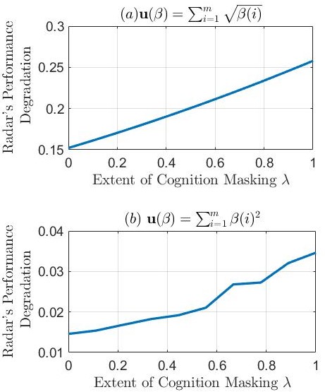
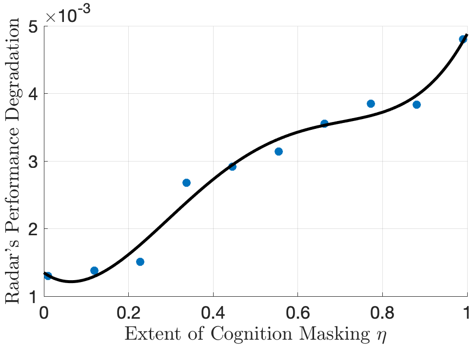
(i) corresponds to maximum cognition masking and hence results in maximum performance loss. (ii) For a fixed value of , the quadratic utility (sub-figure (b)) requires smaller perturbation ( 10 times) from the optimal response compared to the sub-linear utility of sub-figure (a).
Figures 4 and 5 show the performance loss (minimum perturbation from optimal response computed via (15), (17) in Theorem 2) of the cognitive radar as a function of (extent of cognition masking) when the cognitive radar performs waveform adaptation and beam allocation, respectively. We see that for both functionalities, both the radar’s performance loss and adversarial IRL mitigation increase with . This is expected since larger implies a larger shift of the set of feasible strategies computed via IRL to ensure the radar’s strategy is sufficiently close to the edge of the feasible set, at the cost of greater deviation from the radar’s optimal strategy.
V-B Cognition Masking via Theorem 4 for Noisy Adversary Measurements
We now consider the scenario where the adversary has noisy measurements of the radar’s response. Consider the simulation parameters of (37). For our second set of numerical experiments for both waveform adaptation and beam allocation, we set the noise pdf (1) to , where denotes the multivariate normal distribution with mean and covariance , and denotes the identity matrix. In Theorem 4.
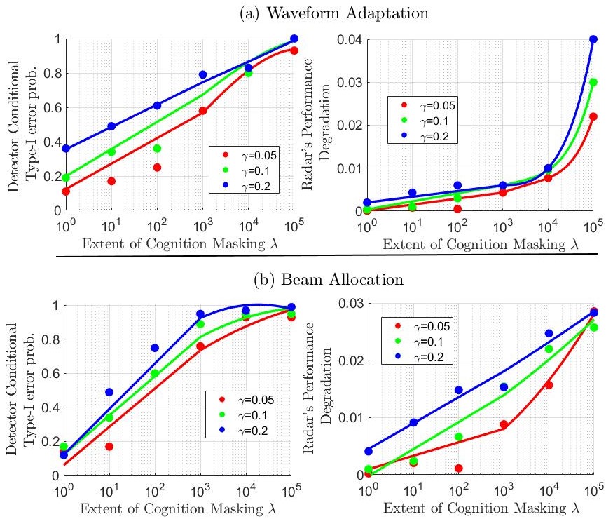
For the noisy case, we consider only a single utility function for waveform adaption, namely, . We performed our numerical experiments for three values of for both waveform adaptation and beam allocation. Recall from Sec. IV that is the significance level of the adversary’s IRL detectors (24) and (25) in Definition 5.
Given the probe sequence , we generated the cognition masking response sequence via (35) for waveform adaption and (36) for beam allocation by varying the parameter (35) over the interval . Recall from Theorem 4 that the radar minimizes the detectors’ conditional Type-I error probability (33), (34) to mitigate adversarial IRL while deliberately compromising on its performance (utility).
Our SPSA algorithm [51, 52] (Algorithm 2) for stochastic gradient descent was executed over iterations for all pairs of , and . Figure 6 shows the conditional Type-I error probability (adversarial IRL mitigation) of the detector and performance loss of the radar as the parameter is varied for three different values of the significance level of the adversary’s detector. Recall from Theorem 4 that the parameter controls the extent of cognition masking for noisy inverse IRL. From Fig. 6, we see that both the conditional Type-I error probability of the IRL detectors and radar’s performance loss increase with as well as .
If , the radar simply transmits its naive response that maximizes its utility (no performance loss) and also results in zero adversarial mitigation. For the limiting case of , the radar’s cognition masking response computed via Theorem 4 degenerates to a constant for all time , hence maximizing the conditional Type-I error probability of the detector at the cost of maximal performance loss for the radar.
Let us briefly discuss the variation of the radar performance and adversarial mitigation as the parameter is varied. (24) can be viewed as the risk-aversion tendency of the adversary’s IRL system since it bounds the detector’s Type-I error probability. Recall from (20) that the Type-I error is the probability of detecting a cognitive radar as non-cognitive. Higher implies the detector is risk-seeking and a lower implies the detector is risk-averse. Naturally, a larger deviation from optimal strategy is required to mitigate a risk-averse detector compared to a risk-seeking detector by the same amount.
Step 1. Set , the naive response sequence (11) that maximizes the radar’s utility (3).
Step 2. Choose (extent of cognition masking).
Step 3. For iterations ,
(i) Compute , the empirical probability estimate of the conditional Type-I error probability of the detector (24) defined in
(33) using fixed realizations of adversary’s measurement noise (1):
| (38) |
In (38):
is a vector of responses
denotes the indicator function
controls the accuracy of the empirical probability estimate
is the distribution function of the r.v. (24)
The statistic is defined in (32).
(ii) Compute empirical estimate of objective :
| (39) |
where is computed in (38).
(ii) Compute the estimate of the gradient as:
where is the gradient step size, denotes the Frobenius norm, and is a random perturbation vector whose each element is with probability .
(iii) Update the radar’s response as:
| (40) |
where is the response update step size and is the projection operator to the hyperplane .
Step 4. Set and go to Step 3.
VI Conclusion and Extensions
This paper investigated how a cognitive radar can hide its cognition from an adversary, when the adversary performs inverse reinforcement learning (IRL) to estimate the radar’s utility function by observing its actions. The adversary’s IRL estimate of the radar’s strategy is a polytope of feasible solutions to a set of convex inequalities. Our first cognition masking result is Theorem 2. When the adversary has accurate measurements of the radar’s response, cognition masking via Theorem 2 ensures the radar’s true strategy lies close to the edge of the feasibility polytope computed via adversarial IRL (true strategy poorly rationalizes adversary’s dataset). When the adversary has noisy measurements of the radar’s response, adversarial IRL generalizes to a cognition detector defined in Definition 5. Our second cognition masking result is Theorem 4. The key idea is to maximize the probability of the radar being classified as non-cognitive by the detector subject to a bound on the radar’s performance loss. Finally, in Sec. V, we illustrate our cognition masking results on a cognitive radar that performs waveform adaptation and beam allocation for target tracking. We show that small purposeful deviations from the optimal strategy of the radar suffice to significantly confuse the adversarial IRL system.
This paper builds significantly on our previous work [4] on ECM for identifying cognitive radars, and [53, 54, 55] on ECCM for masking radar cognition. Theorem 6 extends IRL for cognitive radars [4] when the radar faces multiple resource constraints. The linear IRL feasibility test for a single constraint case generalizes to a mixed integer feasibility test. Theorem 7 generalizes the cognition masking result of [53] to multiple constraints. Our previous works [53, 54, 55] assume optimal adversarial IRL via Afriat’s theorem. This paper generalizes cognition masking to sub-optimal adversarial IRL algorithms. Algorithm 3 outlines a cognition scheme when the adversary uses an arbitrary IRL algorithm to estimate the radar’s strategy. Theorem 8 provides performance bounds for our cognition masking scheme when the adversary has misspecified measurements of the radar’s response. Although this paper is radar-centric, we emphasize that the problem formulation and algorithms developed also apply to adversarial inverse reinforcement learning in general machine learning applications.
Finally, a useful extension of this paper would be to study cognition masking in a dynamic radar-adversary interaction environment in comparison to the batch-wise probe-response exchange considered in this paper. Also, how to mask cognition when the adversary knows of the radar’s ECCM capability? Such an approach warrants a game-theoretic discussion in terms of a Stackelberg game where the adversary moves first and the radar responds to the adversary’s probes. It is also worthwhile exploring state-of-the-art concepts in chance constrained optimization [56] and robust optimization [57, 58] to achieve cognition masking under uncertainty - when the radar has noisy measurements of the adversary’s probes.
-A Feasibility Test for Adversarial IRL
Definition 7 (IRL Feasibility Test).
Consider a dataset of monotone functions and responses . The set of IRL feasibility inequalities is defined as:
| (41) | ||||
| (42) |
where the feasible variable .
Remarks.
1. The IRL feasibility inequalities are linear in the feasible variable . Hence, is a linear feasibility test whose feasibility can be checked using a linear programming solver.
2. The set of inequalities checks for relative optimality [59] between any pair of indices . Consider the abstract setup of the cognitive radar in Definition 2 and suppose Assumption 1 holds. In this context, we define relative optimality as:
| (43) | |||
Eq. 43 states that is the optimal response choice from the finite set and hence a weaker notion of optimality wrt (3). Hence, if Assumption 1 holds, we say wrt utility , the dataset satisfies relative optimality. The feasibility of the IRL inequalities (41) is equivalent (due to [9]) to the existence of a utility function such that relative optimality holds.
3. Finally, let us provide some intuition on the feasible variable in (41). Suppose (41). On inspecting (42) in more detail, the first components of the vector can be viewed as the utility function corresponding to the feasible variable evaluated at responses
. The last components can be viewed as the Lagrange multipliers associated with the Lagrangian of the optimization problem over all . In summary, we have the following correspondence between the feasible variable and the feasible utility function :
| (44) |
where the division operation in (44) is element-wise.
4. The interpretation of the feasibility vector in (44) facilitates us to define the mapping as:
| (45) |
It is straightforward to show that both relative optimality (43) and absolute optimality (3) hold for (45) if . Also, for any utility function and dataset (41), define the reverse mapping as:
| (46) |
Then, it is straightforward to show:
| (47) |
where is defined in (46) and can be interpreted as the finite dimensional projection of for the IRL feasibility test .
-B IRL for Identifying Radar’s Resource Constraint
Theorem 5 (IRL for Identifying Resource Constraint).
-C Example. Optimal Waveform Adaptation
Consider the radar-adversary interaction of Definition 1. Suppose the radar uses a Bayesian tracker (Kalman filter) for estimating the target’s state, and suppose the adversary’s probe and radar’s response parameterize the radar’s state and observation noise covariances, respectively. We assume is the measurement precision (amount of directed energy) of the radar in the mode, and probe is the radar’s incentive for considering the mode of the target. Specifically, probe is the vector of eigenvalues of the state noise covariance matrix , and response is the vector of eigenvalues of the inverse of the observation noise covariance matrix in the linear Gaussian dynamics model of (2).
Our working assumption is that the radar is cognitive, and maximizes a utility subject to an operating constraint . For optimal waveform adaptation, we assume the operating constraint is a bound on the inverse of the radar tracker’s asymptotic covariance , where is the solution of the algebraic Ricatti equation. As justified below, a bounded asymptotic precision is equivalent to the linear constraint .
Kalman filter-based Bayesian Tracker. Suppose the radar estimates the target state with covariance from observations . The posterior is propagated recursively in time via the classical Kalman filter equations:
Assuming the model parameters (2) satisfy the conditions that is detectable and is stabilizable, the steady-state predicted covariance is the unique positive semi-definite solution of the algebraic Riccati equation (ARE):
| (50) |
Let denote the solution of the ARE (50). Our working assumption is that the radar can only expend sufficient resources to ensure that the precision (inverse covariance) is at most some pre-specified precision at each epoch and then choose the ‘best’ waveform (equivalently, observation covariance) available. Such trade-offs for the radar arise frequently in cognitive radar models in literature [2, 3]777In [2], the radar minimizes the mean-squared error of the target’s estimate subject to a Cramer-Rao bound on the target’s localization accuracy. In [3], the radar minimizes its posterior Cramer-Rao bound, subject to an upper bound on its transmission power and antenna deployment cost. We now invoke [4, Lemma 3] and show the equivalence between the complex non-linear constraint and the linear constraint . The key idea in [4, Lemma 3] is to show the asymptotic precision is monotone increasing in the second argument using the information Kalman filter formulation [60]. To summarize, the radar’s optimal waveform adaptation strategy can be expressed as:
| (51) |
Remark. The RHS in the constraint in (51) can be set to 1 WLOG by appropriately scaling the probe signal .
-D Example. Optimal Beam Allocation
For abstracting beam allocation into a constrained utility maximization setup (3), we work at a higher level of abstraction compared to waveform adaptation. Specifically, we assume the adversary comprises multiple targets. At this higher level of abstraction, we view each component of the adversarial probe signal as the trace of the predicted precision matrix (inverse covariance) of target . Recall from the previous section that we used the probe signal (11) to parametrize the maneuver covariance matrix. In comparison, we now use the trace of the precision of each target in our probe signal – this allows us to consider multiple targets.
Multiple Target-tracking. For the optimal beam allocation example, we assume the adversary comprises a collection of adversarial targets indexed by . We assume the cognitive radar adaptively switches its beam between the targets. As in (2), on the fast time scale indexed by , target has linear Gaussian dynamics and the radar obtains linear Gaussian measurements of the targets’ maneuvers:
| (52) |
Here , . We assume that both and are known to the radar and adversary. As in the previous sub-section, indexes the slow time scale and indexes the fast time scale. For target , the radar’s Kalman covariance The enemy’s radar tracks our targets using Kalman filter trackers.
Probe-Response Parametrization. The target’s predicted precision parametrizes the element of the adversary’s probe. Specifically, the price the radar pays at the start of epoch for tracking target is the trace of the inverse of the predicted covariance at epoch using the Kalman predictor:
| (53) |
where is the covariance of the target’s covariance at time (fast time scale) in epoch . Clearly, the predicted covariance (53) is a deterministic function of the maneuver covariance of target . The radar’s response to the adversary’s probe is the beam intensity allocated to target in epoch . Intuitively, at the start of every epoch , the radar computes the predicted precision of the state estimate of target , and then chooses the beam intensity towards target during epoch . The radar can at best compute the predicted precision for its decision (since it has no access to observations at the beginning of the epoch).
Optimal beam allocation. We assume that the radar, at epoch , faces a resource constraint and directs beam intensities towards targets , respectively. We assume the radar’s resource constraint can be expressed as , the -norm of the radar’s response. The radar’s aim is to maximize the Cobb-Douglas utility of the transmitted intensities:
| (54) |
The exponents for the Cobb-Douglas utility function (54), referred to as elasticity parameters in consumer economics literature, parameterize the marginal utility per consumer good. In complete analogy, the elasticity parameters in our cognitive radar context parameterize the incentive for the radar to focus its beam towards a particular target. The economic rationale for the cognitive radar is as follows - a higher predicted precision for target implies a better state estimate, and thus a higher incentive for the radar to direct its transmission intensity towards target . To summarize, the cognitive radar’s beam allocation functionality can be abstracted as:
| (55) | |||
Eq. 12 abstracts the beam allocation functionality of the cognitive radar; at time the radar maximizes a Cobb-Douglas888 The Cobb-Douglas utility function is widely used in microeconomics to model human satisfaction from buying consumer goods. In the radar context, this utility function measures the performance of the cognitive radar. utility (utility specified by the adversarial target) subject to a constraint on the -norm of its response (beam intensity allocation). In the beam allocation case, the aim of adversarial IRL is to estimate the scalar that parametrizes the radar’s budget constraint .
In (12), notice how the adversary’s probe parametrizes the radar’s utility function instead of its budget constraint as in (11). Also, observe that both the utility function and cost are monotone in the transmission intensities - higher beam intensity yields a larger utility but is also more costly. We assume that: (1) each target is equipped with a radar detector and can estimate the beam intensity the enemy’s radar directs towards it - this assumption facilitates the targets to carry out adversarial IRL attacks on the radar, and (2) the adversarial targets know the radar is maximizing the Cobb-Douglas utility function (54), but does not know the radar’s budget constraint and is the adversary’s IRL objective in the beam allocation context as discussed below.
IRL for optimal beam allocation. We now present Theorem 1, a revealed preference-based IRL algorithm for the adversary. Unlike Theorem 1, the adversary parametrizes (and hence, knows) the utility function of the cognitive radar, but does not know its budget constraint. Hence, the IRL objective of the adversarial target in Theorem 1 is to estimate the radar’s budget .
-E Proof of Theorem 31
Proof.
The Type-I error probability is given by , that is, probability that the adversary misclassifies a utility maximizer as not a utility maximizer. Let us first consider the statistical test (24) in Definition 5. Assume holds. Then, the Afriat inequalities (6) for the true dataset to have a feasible solution. Let denote any feasible solution to Afriat’s inequalities (6). Then, the following inequalities result:
| (56) |
Since the test statistic (28) is the minimum perturbation needed for the feasibility of Afriat’s inequalities (6), (56) yields the following inequality:
| (57) |
The Type-I error probability can now be bounded as:
Hence, the Type-I error probability of the statistical test (24) is bounded by its significance level . Showing the Type-I error probability of the detector (25) is bounded is identical to the steps outlined above, and thus, omitted. ∎
-F Masking Radar’s Utility Function for Multiple Constraints
Our IRL results for estimating the radar’s utility (3) assumes a scalar-valued budget constraint for the radar. In general, the radar faces multiple constraints, or equivalently, the constraint is vector-valued. How to generalize Theorem 1 to vector-valued constraints? In this section, we generalize our IRL algorithm (Theorem 1) and cognition masking results of Theorem 2 to vector-valued when the adversary knows the radar’s constraints and estimates the radar’s utility - this scenario is formalized below in assumption 5. Generalizing IRL for identifying a vector-valued constraint is non-identifiable and hence, omitted.
Assumption 5.
The radar’s resource constraint in (3) is vector-valued, and the radar’s utility is independent of :
| (58) |
where is the dimension of the probe/response, and is a scalar-valued constraint.
IRL objective. The adversary aims to reconstruct the radar’s utility using the dataset , where is defined in (5).
Assumption 5 specializes to assumption 1 when is scalar-valued and linear in both the probe and response vectors. Let us now state Theorem 6 for achieving IRL for vector-valued constraints when assumption 5 holds.
Theorem 6 (IRL for Identifying Radar’s Utility Function for Vector-Valued Constraints).
Consider the cognitive radar described in Definition 1. Suppose assumption 1 holds. Then:
(a) The adversary checks for the existence of a feasible utility function that satisfies (3) by checking the feasibility of the following set of inequalities:
| (59) | |||
| (60) | |||
where dataset is defined in (5).
(b) If (59) has a feasible solution, the set-valued IRL estimate of the radar’s utility is given by:
| (61) |
where is any feasible solution to the inequalities (59), (60).
Remarks.
1. In comparison to the linear feasibility test (6) of Theorem 1, (59) in Theorem 6 is a mixed-integer linear feasibility test, mixed-integer due to the second set of inequalities (60) in the feasibility test.
2. Afriat’s theorem 6 requires that the constraint be active at the solution, meaning for all . This requirement is implicitly satisfied for the scalar case due to the monotonicity of both the utility and constraint . For vector-valued , however, requiring all constraints to be active at the solution is highly restrictive. That is, for all time steps and constraint indices is not true in general for a cognitive radar. Hence, the IRL inequalities for multiple constraints must account for the inactive constraints for all time steps . More precisely, the inverse learner needs to check for at least one active constraint out of all resource constraints for all . This is ensured by the feasibility of (60) in Theorem 6. At a deeper level, (60) tests for complementary slackness in the KKT conditions [61, Sec. 5.5] for first-order optimality of the radar’s responses.
3. In Afriat’s theorem (Theorem 1), the reconstructed utility function (7) is a point-wise minimum of scaled and shifted versions of the radar’s linear constraints . Intuitively, the basis functions for the adversary’s estimate of the radar’s utility are the radar’s constraints . For the multiple constraints case in Theorem 6 above, the adversary’s utility estimate has a richer representation due to a larger set of basis functions .
Having defined our IRL algorithm for multiple constraints in Theorem 6 above, we now present our cognition masking result for mitigating the IRL procedure of Theorem 6.
Definition 8 (Feasibility Margin for Reconstructed Utility (6) for Multiple Constraints).
The margin definition in (62) above is a multi-constraint generalization of Definition 3. To glean some insight into the notation in (62) above, consider the simple case where . Then, the solution to is simply the Lagrange multiplier associated with the single operating constraint in the optimization problem (3). For the multiple constraint case, the solution to is the vector of Lagrange multipliers for the constraints at (3), the optimal response at time . Denoting the IRL feasibility test wrt inequalities (59) and (60) as , the margin for any utility when is vector-valued can be compactly defined as:
| (63) |
Having generalized the margin definition of (13) in Definition 3 to the multiple constraint case, we now state our cognition masking result, Theorem 7 for vector-valued . The cognition masking rationale for vector-valued remains the same as that in Theorem 2: add engineered noise to the radar’s optimal responses, and ensure the radar’s utility lies sufficiently close to the edge of the feasibility polytope of viable utilities computed via IRL.
Theorem 7 (Masking Utility from Adversarial IRL for Multiple Resource Constraints.).
Consider the cognitive radar (3) from Definition 2 with multiple resource constraints (assumption 5 holds). Let denote the naive response sequence (3) that maximizes the cognitive radar’s utility. The response sequence defined below masks the radar’s utility from the adversary by ensuring satisfies the IRL inequalities (59), (60) with a sufficiently low margin (62):
| (64) | ||||
| (65) |
where dataset is the adversary’s dataset when the radar transmits naive responses , and is defined in (5).
-G Cognition Masking Performance under Misspecified Radar Response Measurements
In this section, we investigate how the performance of the radar’s cognition masking algorithm, Theorem 2, changes when the adversary has misspecified measurements of the radar’s responses. By misspecified responses, we mean the true radar response is corrupted by an additive deterministic perturbation , . Misspecified response measurements formalized in assumption 6 below are different from noisy measurements since the perturbation is a deterministic vector and not a random variable like in the noisy case considered in Sec. IV.
Assumption 6 (Misspecified Radar Response Measurements).
Suppose the adversary has misspecified measurements of the radar’s response . Assume the misspecifications have a bounded -norm:
| (66) |
The adversary’s misspecified datasets and are defined as:
| (67) |
where is the radar’s response at time , and are the utility and constraint, respectively, of the cognitive radar (3).
Recall from Theorem 2 that the positive scalar parametrizes the extent of cognition masking by the cognitive radar. Our key objective is to derive a lower bound on the effective extent of cognition masking defined as:
| (68) |
where (67) are the misspecified datasets of the adversary if the radar transmits naive responses (3), and are the misspecified datasets when the radar transmits cognition masking responses computed via (15) and (17), respectively. The variable (68) is the ratio between the margins of the radar’s strategy (utility or constraint ) (13), (14) with and without the radar’s cognition masking scheme (Theorem 2) when the adversary has misspecified response measurements. It is easy to see that if the misspecification error (67) is for all . For non-zero , Theorem 8 below yields a lower bound for and uses the following variables (given assumption 6 holds):
| (69) |
The variables defined in (69) measure the deviation in the radar’s utility and constraint values evaluated at the misspecified radar responses measured by the adversary, compared to the utility and constraint evaluations at the true radar responses. We are now ready to state Theorem 8.
Theorem 8 (Performance of Cognition Masking (Theorem 2) for Misspecified Responses).
Consider the cognition masking scheme of Theorem 2. Assume the adversary has misspecified radar response measurements (assumption 6 holds).
Then:
(i) Suppose assumption 1 holds, i.e. , the adversary knows the radar’s constraint . Then, the effective extent of cognition masking is bounded from below as:
| (70) |
(ii) Suppose assumption 2 holds, i.e. , the adversary knows the radar’s constraint . Then, the effective extent of cognition masking is bounded from below as:
| (71) |
The variables measure the distortion in the adversary’s dataset due to misspecified measurements and defined in (69).
Theorem 8 computes a lower bound on the effectiveness of the cognitive masking scheme of Theorem 2 when the adversary has misspecified measurements of the radar’s response. The proof for Theorem 8 is omitted for brevity. Observe that the bounds in (70), (71) are inversely proportional to the quantities and . These quantities can be interpreted as the ‘spread’ in the utility and constraint evaluations at the radar’s true responses due to the misspecification errors (67) and, in turn, are proportional to (66), the maximum norm of . Hence, we can conclude the lower bound for the effectiveness of the radar’s cognition masking scheme worsens with the magnitude of the misspecification errors in the adversary’s measurements.
-H Cognition Masking for Arbitrary IRL Algorithm
Our cognition masking results of Theorems 2 and 4 assume the adversary performs optimal IRL via Afriat’s theorem (Theorems 1 and 5) to reconstruct the radar’s strategy. However, our cognition masking results can be straightforwardly extended to any IRL algorithm. Any IRL algorithm can be expressed WLOG as a set-valued estimation algorithm that generates a set of feasible strategies given a finite dataset of adversary probes and radar responses :
| (72) |
In (72), parametrizes the reconstructed utility, is the adversary’s dataset and is the number of IRL feasibility inequalities. In Afriat’s theorem, for example, and . Algorithm 3 below outlines the steps for mitigating an arbitrary IRL algorithm . Recall Theorem 2 minimizes the feasibility margin of the radar’s strategy wrt the Afriat inequalities (6), (48) by deliberately perturbing the radar’s responses. In complete analogy, a radar can hide its strategy from any set-valued IRL estimation scheme by minimizing the feasibility margin defined below in (73) wrt the IRL feasibility inequalities by purposefully injecting noise in the radar’s responses. Due to the non-linear margin constraint in (74), the optimization problem can be solved using a general purpose non-linear programming solver, for example, fmincon in MATLAB, to obtain a local minimum.
Step 1. Compute radar’s naive response sequence by solving the convex optimization problem (3):
where is concave monotone in and is convex monotone in .
Step 2. Choose (extent of cognition masking from IRL feasibility test).
Step 3. Compute the margin of the naive responses wrt the IRL algorithm:
| (73) |
where is a vector of all ones and is the radar’s utility.
Step 3. Compute upper bound on desired margin (13) after cognition masking:
.
Step 4. Compute the cognition-making response sequence by solving the following optimization problem:
| (74) |
References
- [1] K. V. Mishra, M. B. Shankar, and B. Ottersten. Toward metacognitive radars: Concept and applications. In 2020 IEEE International Radar Conference (RADAR), pages 77–82. IEEE, 2020.
- [2] X. Wang, Z. Fei, J. A. Zhang, J. Huang, and J. Yuan. Constrained utility maximization in dual-functional radar-communication multi-uav networks. IEEE Transactions on Communications, 69(4):2660–2672, 2020.
- [3] P. Chavali and A. Nehorai. Scheduling and power allocation in a cognitive radar network for multiple-target tracking. IEEE Transactions on Signal Processing, 60(2):715–729, 2012.
- [4] V. Krishnamurthy, D. Angley, R. Evans, and B. Moran. Identifying cognitive radars - inverse reinforcement learning using revealed preferences. IEEE Transactions on Signal Processing, 68:4529–4542, 2020.
- [5] V. Krishnamurthy, K. Pattanayak, S. Gogineni, B. Kang, and M. Rangaswamy. Adversarial radar inference: Inverse tracking, identifying cognition, and designing smart interference. IEEE Transactions on Aerospace and Electronic Systems, 57(4):2067–2081, 2021.
- [6] A. Y. Ng, S. J. Russell, et al. Algorithms for inverse reinforcement learning. In Icml, volume 1, page 2, 2000.
- [7] P. Abbeel and A. Y. Ng. Apprenticeship learning via inverse reinforcement learning. In Proceedings of the twenty-first international conference on Machine learning, page 1, 2004.
- [8] B. D. Ziebart, A. L. Maas, J. A. Bagnell, A. K. Dey, et al. Maximum entropy inverse reinforcement learning. In Aaai, volume 8, pages 1433–1438. Chicago, IL, USA, 2008.
- [9] S. Afriat. The construction of utility functions from expenditure data. International economic review, 8(1):67–77, 1967.
- [10] A. Caplin and M. Dean. Revealed preference, rational inattention, and costly information acquisition. The American Economic Review, 105(7):2183–2203, 2015.
- [11] J. A. Boyd, D. B. Harris, D. D. King, and H. Welch Jr. Electronic countermeasures. Electronic Countermeasures, 1978.
- [12] A. Kuptel. Counter unmanned autonomous systems (cuaxs): Priorities. policy. future capabilities. Policy. Future Capabilities (May 5, 2017). Multinational Capability Development Campaign (MCDC), pages 15–16, 2017.
- [13] C. Shi, F. Wang, M. Sellathurai, and J. Zhou. Low probability of intercept-based distributed mimo radar waveform design against barrage jamming in signal-dependent clutter and coloured noise. IET Signal Processing, 13(4):415–423, 2019.
- [14] F. A. Butt, I. H. Naqvi, and U. Riaz. Hybrid phased-mimo radar: A novel approach with optimal performance under electronic countermeasures. IEEE Communications Letters, 22(6):1184–1187, 2018.
- [15] S. Gong, X. Wei, and X. Li. Eccm scheme against interrupted sampling repeater jammer based on time-frequency analysis. Journal of Systems Engineering and Electronics, 25(6):996–1003, 2014.
- [16] H. Varian. Revealed preference and its applications. The Economic Journal, 122(560):332–338, 2012.
- [17] V. Krishnamurthy and W. Hoiles. Afriat’s test for detecting malicious agents. IEEE Signal Processing Letters, 19(12):801–804, 2012.
- [18] K. Amin, R. Cummings, L. Dworkin, M. Kearns, and A. Roth. Online learning and profit maximization from revealed preferences. In Proceedings of the AAAI Conference on Artificial Intelligence, volume 29-1, 2015.
- [19] A. Roth, J. Ullman, and Z. S. Wu. Watch and learn: Optimizing from revealed preferences feedback. In Proceedings of the forty-eighth annual ACM symposium on Theory of Computing, pages 949–962, 2016.
- [20] Y. Sakuma, T. P. Tran, T. Iwai, A. Nishikawa, and H. Nishi. Trajectory anonymization through laplace noise addition in latent space. In 2021 Ninth International Symposium on Computing and Networking (CANDAR), pages 65–73, 2021.
- [21] C. Shi, F. Wang, M. Sellathurai, and J. Zhou. Low probability of intercept-based distributed mimo radar waveform design against barrage jamming in signal-dependent clutter and coloured noise. IET Signal Processing, 13(4):415–423, 2019.
- [22] D. Schleher. Lpi radar: fact or fiction. IEEE Aerospace and Electronic Systems Magazine, 21(5):3–6, 2006.
- [23] P. E. Pace. Detecting and classifying low probability of intercept radar. Artech house, 2009.
- [24] J. Akhtar. Orthogonal block coded eccm schemes against repeat radar jammers. IEEE Transactions on Aerospace and Electronic Systems, 45(3):1218–1226, 2009.
- [25] M. Soumekh. Sar-eccm using phase-perturbed lfm chirp signals and drfm repeat jammer penalization. In IEEE International Radar Conference, 2005., pages 507–512. IEEE, 2005.
- [26] D. S. Garmatyuk and R. M. Narayanan. Eccm capabilities of an ultrawideband bandlimited random noise imaging radar. IEEE Transactions on Aerospace and Electronic Systems, 38(4):1243–1255, 2002.
- [27] N. D. Ratliff, J. A. Bagnell, and M. A. Zinkevich. Maximum margin planning. In Proceedings of the 23rd international conference on Machine learning, pages 729–736, 2006.
- [28] Y. Bar-Shalom, X. R. Li, and T. Kirubarajan. Estimation with applications to tracking and navigation. John Wiley, New York, 2008.
- [29] X. R. Li and V. P. Jilkov. Survey of maneuvering target tracking. part i. dynamic models. IEEE Transactions on Aerospace and Electronic Systems, 39(4):1333–1364, 2003.
- [30] S. Blackman and R. Popoli. Design and Analysis of Modern Tracking Systems. Artech House, 1999.
- [31] S. Haykin. Cognitive radar: a way of the future. IEEE signal processing magazine, 23(1):30–40, 2006.
- [32] K. L. Bell, C. J. Baker, G. E. Smith, J. T. Johnson, and M. Rangaswamy. Cognitive radar framework for target detection and tracking. IEEE Journal of Selected Topics in Signal Processing, 9(8):1427–1439, 2015.
- [33] F. Forges and E. Minelli. Afriat’s theorem for general budget sets. Journal of Economic Theory, 144(1):135–145, 2009.
- [34] Y. Liu, G. Liao, Z. Yang, and J. Xu. Multiobjective optimal waveform design for ofdm integrated radar and communication systems. Signal Processing, 141:331–342, 2017.
- [35] D. J. Kershaw and R. J. Evans. Optimal waveform selection for tracking systems. IEEE Transactions on Information Theory, 40(5):1536–1550, 1994.
- [36] S. Haykin, Y. Xue, and T. N. Davidson. Optimal waveform design for cognitive radar. In 2008 42nd Asilomar Conference on Signals, Systems and Computers, pages 3–7. IEEE, 2008.
- [37] E. Grossi and M. Lops. MIMO radar waveform design: a divergence-based approach for sequential and fixed-sample size tests. In 3rd IEEE International Workshop on Computational Advances in Multi-Sensor Adaptive Processing, pages 165–168, 2009.
- [38] V. Krishnamurthy and R. Evans. Hidden Markov model multi-arm bandits: A methodology for beam scheduling in multi-target tracking. IEEE Transactions on Signal Processing, 49(12):2893–2908, December 2001.
- [39] V. Krishnamurthy. Partially Observed Markov Decision Processes. From Filtering to Controlled Sensing. Cambridge University Press, 2016.
- [40] V. Krishnamurthy and D. Djonin. Optimal threshold policies for multivariate POMDPs in radar resource management. IEEE Transactions on Signal Processing, 57(10), 2009.
- [41] M. Xie, W. Yi, L. Kong, and T. Kirubarajan. Receive-beam resource allocation for multiple target tracking with distributed mimo radars. IEEE Transactions on Aerospace and Electronic Systems, 54(5):2421–2436, 2018.
- [42] J. Wang and H. Zhu. Beam allocation and performance evaluation in switched-beam based massive mimo systems. In 2015 IEEE International Conference on Communications (ICC), pages 2387–2392. IEEE, 2015.
- [43] J. Wang, H. Zhu, L. Dai, N. J. Gomes, and J. Wang. Low-complexity beam allocation for switched-beam based multiuser massive mimo systems. IEEE Transactions on Wireless Communications, 15(12):8236–8248, 2016.
- [44] H. R. Varian et al. Goodness-of-fit for revealed preference tests. Citeseer, 1991.
- [45] M. Dean and D. Martin. Measuring rationality with the minimum cost of revealed preference violations. Review of Economics and Statistics, 98(3):524–534, 2016.
- [46] F. Echenique, S. Lee, and M. Shum. The money pump as a measure of revealed preference violations. Journal of Political Economy, 119(6):1201–1223, 2011.
- [47] M. Dean and D. Martin. Measuring rationality with the minimum cost of revealed preference violations. Review of Economics and Statistics, 98(3):524–534, 2016.
- [48] B. Smeulders, F. C. Spieksma, L. Cherchye, and B. De Rock. Goodness-of-fit measures for revealed preference tests: Complexity results and algorithms. ACM Transactions on Economics and Computation (TEAC), 2(1):1–16, 2014.
- [49] B. E. Boser, I. M. Guyon, and V. N. Vapnik. A training algorithm for optimal margin classifiers. In Proceedings of the fifth annual workshop on Computational learning theory, pages 144–152, 1992.
- [50] H. V. Trees. Detection, Estimation and Modulation Theory. John Wiley & Sons, 1968.
- [51] J. Spall. Introduction to Stochastic Search and Optimization. Wiley, 2003.
- [52] I.-J. Wang and J. C. Spall. A constrained simultaneous perturbation stochastic approximation algorithm based on penalty functions. In Proceedings of the 1999 American Control Conference (Cat. No. 99CH36251), volume 1, pages 393–399. IEEE, 1999.
- [53] K. Pattanayak, V. Krishnamurthy, and C. Berry. How can a cognitive radar mask its cognition? In ICASSP 2022-2022 IEEE International Conference on Acoustics, Speech and Signal Processing (ICASSP), pages 5897–5901. IEEE, 2022.
- [54] K. Pattanayak, V. Krishnamurthy, and C. Berry. Meta-cognition. an inverse-inverse reinforcement learning approach for cognitive radars. arXiv preprint arXiv:2205.01794, 2022.
- [55] K. Pattanayak, V. Krishnamurthy, and C. Berry. Inverse-inverse reinforcement learning. how to hide strategy from an adversarial inverse reinforcement learner. arXiv preprint arXiv:2205.10802, 2022.
- [56] A. Nemirovski and A. Shapiro. Scenario approximations of chance constraints. Probabilistic and randomized methods for design under uncertainty, pages 3–47, 2006.
- [57] A. Ben-Tal, L. El Ghaoui, and A. Nemirovski. Robust optimization, volume 28. Princeton university press, 2009.
- [58] H.-G. Beyer and B. Sendhoff. Robust optimization–a comprehensive survey. Computer methods in applied mechanics and engineering, 196(33-34):3190–3218, 2007.
- [59] K. Pattanayak, V. Krishnamurthy, and E. Blasch. Inverse sequential hypothesis testing. In 2020 IEEE 23rd International Conference on Information Fusion (FUSION), pages 1–7. IEEE, 2020.
- [60] B. D. O. Anderson and J. B. Moore. Optimal filtering. Prentice Hall, Englewood Cliffs, New Jersey, 1979.
- [61] S. Boyd and L. Vandenberghe. Convex Optimization. Cambridge University Press, 2004.