Point pattern analysis and classification on compact two–point homogeneous spaces evolving time

Abstract

This paper introduces a new modeling framework for the statistical analysis of point patterns on a manifold $\mathbb{M}_{d},$ defined by a connected and compact two–point homogeneous space, including the special case of the sphere. The presented approach is based on temporal Cox processes driven by a $L^{2}(\mathbb{M}_{d})$–valued log–intensity. Different aggregation schemes on the manifold of the spatiotemporal point–referenced data are implemented in terms of the time–varying discrete Jacobi polynomial transform of the log–risk process. The $n$–dimensional microscale point pattern evolution in time at different manifold spatial scales is then characterized from such a transform. The simulation study undertaken illustrates the construction of spherical point process models displaying aggregation at low Legendre polynomial transform frequencies (large scale), while regularity is observed at high frequencies (small scale). $K$–function analysis supports these results under temporal short–, intermediate– and long–range dependence of the log–risk process.

Keywords: Connected and compact two–point homogeneous spaces; Cox processes; discrete Jacobi polynomial transform; $K$–function; $\mathbb{M}_{d}$–supported random fields; point pattern analysis; statistical distances.

1 Introduction

Several statistical approaches arise for processing spatial areally-aggregated or/and misalignment data in several environmental disciplines requiring, for example, the application of Geophysical, Ecological and Epidemiological models. The approach presented in this paper goes beyond the Euclidean setting, analyzing count models on a manifold defined by a connected and compact two–point homogeneous space. Under spatial isotropy we consider weighted aggregation schemes adapted to the geometry of the manifold, in terms of the elements of the Jacobi polynomial basis (see Theorems 4 and 5 in [22], and [23] for the special case of the sphere). The application of harmonic analysis in this more general context leads to the characterization of the evolution of point patterns at different spatial scales in the manifold.

Markov random field (MRF) models, particularly, Conditional Autoregressive (CAR) models have been widely applied to represent the dynamics of the log–intensity process, interpreted as a log–risk process in the context of double stochastic Poisson processes, also named Cox processes (see [5]). In disease mapping, areal disease counts have been usually analyzed under this Markovian log–risk process framework (see, e.g., [32]; [33]; [34]). Particularly, different parametric, semiparametric and nonparametric statistical approaches have been adopted in the estimation of deterministic and random intensities (see [4]; [13]; [16]; [17], and the references therein). In point pattern analysis, special attention has been paid to functional summary statistics like the nearest neighbour, empty space, and $K$ functions (see, e.g., [11];[19]). Recently, LASSO estimation based on spherical autoregressive processes has been proposed in [8] beyond the Euclidean setting.

Alternatively, in the functional data analysis (FDA) framework, conditional autoregressive Hilbertian process (CARH process) models were considered by [9], [10] and [18], developing projection estimation methods for prediction. In [28], an Autoregressive Hilbertian process (ARH(1) process) framework was adopted to represent the dynamics of the spatiotemporal log–risk process. This framework has also been adopted in [31] for COVID–19 mortality prediction by applying multivariate curve regression and machine learning. As an alternative, to analyze the spatial interaction between log–risk curves at different regions, in [15], a Spatial Autoregressive Hilbertian process (SARH(1) process) based modeling was applied. Recently, wavelet–based projection methods are implemented in [30] to developing an infinite–dimensional spatial multiresolution point pattern analysis, based on spatiotemporal Log-Gaussian Cox processes in the Euclidean setting. The present paper goes beyond this Euclidean setting. At each spatial resolution level on the manifold, defined in terms of time–varying discrete Jacobi transform, temporal point pattern analysis is achieved from the latent random intensity process in time, and its higher order moments. In the particular case of the sphere, suitable log–intensity models can be found in [7], where spherical functional autoregressive (SPHAR) processes are introduced, and their asymptotically analysis is derived. Additionally, spherical functional autoregressive–moving average (SPHARMA) processes are considered in [6], extending SPHAR processes, for suitable approximation of isotropic and stationary sphere–cross–time random fields. Here, functional spectral analysis tools are applied, and Wold–like decomposition results are derived.

A growing interest on spherical point processes, and its functional summary statistics is observed in recent contributions (see, e.g., [26]; [27]). In this paper, our interest relies on point patterns analysis in compact two–point homogeneous spaces evolving time. The framework of temporal Cox processes driven by log–intensities, evaluated in the space $L^{2}(\mathbb{M}_{d},d\nu)$ of square integrable functions on a compact two–point homogeneous space $\mathbb{M}_{d}$ is then considered. Particularly, $\mathbb{M}_{d}$ is a manifold with $d$ denoting its topological dimension, and $d\nu$ denotes its measure, induced by the probabilistic invariant measure on the connected component of the group of isometries of $\mathbb{M}_{d}.$ The associated infinite–dimensional $n$–order product density is identified with the infinite product of temporal $n$–order product densities. A spatial multi–scale analysis of the point process evolution is achieved from these temporal $n$–order product densities, and the usual functional summary statistics constructed from them.

The interest of the extended family of Cox processes analyzed here relies on well–known examples of compact two–point homogeneous spaces like the sphere $\mathbb{S}_{d}\subset\mathbb{R}^{d+1},$ and the projective spaces over different algebras (see Section 2 in [22] for more details). Recent advances on modeling, analysis and simulation of Gaussian spherical isotropic random fields, including random fields obeying a fractional stochastic partial differential equation on the sphere, can be exploited in our more general $L^{2}(\mathbb{M}_{d},d\nu)$–valued Gaussian log–risk process framework (see [1]; [3]; [14]; [21], among others). Particularly, [3] and [21] focalize on Cosmic Microwave Background (CMB) evolution modeling and data analysis. The approach presented here can contribute to this modeling framework to approximate the distribution of CMB hot and cold spots.

In point pattern analysis on a $d$–dimensional manifold $\mathbb{M}_{d},$ embedded into $\mathbb{R}^{d+1},$ one can apply the isometric identification of $(\mathbb{S}_{d},d_{\mathbb{S}_{d}})$ with $(\mathbb{M}_{d},d_{\mathbb{M}_{d}})$ via the identity $d_{\mathbb{S}_{d}}(\mathbf{x}_{1},\mathbf{x}_{2})=\arccos\left(\mathbf{x}_{1}^{T}\mathbf{x}_{2}\right),$ for $\mathbf{x}_{1},\mathbf{x}_{2}\in\mathbb{S}_{d}.$ This geodesic distance $d_{\mathbb{M}_{d}}$ is involved in the definition of functional summary statistics characterizing the aggregation, regularity or inhibition of the point pattern. In particular, point pattern classification is achieved in terms of this geodesic distance. This paper presents a new manifold spatial–scale–dependent point pattern classification analysis over time, via time–varying discrete Jacobi transform, achieved in terms of different statistical distances. $K$ function analysis is also performed describing the cumulative counting properties of pair correlation function in time through different spatial scales. In the simulation study undertaken on the sphere, temporal short–, intermediate– and long–range dependence models are tested, the statistical distance based methods implemented reflect a departure from complete randomness of the point pattern at coarser (large) scales in the manifold (low frequencies of the time–varying discrete Legendre polynomial transform). While their small scale (high–frequency) behavior shows regularity. $K$–function based analysis supports the same classification results, independently of the underlying dependence range of the log–intensity. At coarser spatial scales, stronger departure from point pattern regularity is observed when long–range dependence log–intensity models are tested. As mentioned above, the approach presented in this paper then provides a framework to detect non–uniformity of the spherical distribution of CMB hot and cold spots, since these deviations from uniformity are usually geometrically described in terms of clustering, girdling or ring structures (see, e.g., [20]; [29]).

The outline of the paper is the following. Preliminaries on connected and compact two–point homogeneous spaces are given in Section 2. The new class of Cox processes analyzed in a metric space framework is introduced in Section 3. The proposed statistical distance based classification methodology through spatial scales, involving $n$–order product density, is formulated in Section 4. $K$ function is also explicitly computed from the time–varying discrete Jacobi transform of the second–order structure of the $L^{2}(\mathbb{M}_{d})$–valued temporal log–intensity. The results of the simulation study undertaken are displayed in Section 5. Some final remarks and discussion can be found in Section 6 to ending the paper.

2 Preliminaries

Let $\{X_{t}(\cdot),\ t\in\mathcal{T}\subseteq\mathbb{R}\}$ be an infinite–dimensional random process such that, for each $t\in\mathcal{T}\subseteq\mathbb{R},$ almost surely $\log(X_{t})\in L^{2}(\mathbb{M}_{d}),$ and $E[\log(X_{t})]\underset{L^{2}(\mathbb{M}_{d})}{=}0,$ with $\log(X_{t})$ having characteristic functional

$$f_{\log(X_{t})}(h) = \int_{L^{2}(\mathbb{M}_{d})}\exp\left(i\left\langle h,\log(x_{t})\right\rangle_{L^{2}(\mathbb{M}_{d})}\right)\mu_{\log(X_{t})}(d\log(x_{t}))$$ (1)

$$= \exp\left(-\frac{\left\langle\mathcal{R}_{0}(h),h\right\rangle_{L^{2}(\mathbb{M}_{d})}}{2}\right),\quad h\in L^{2}(\mathbb{M}_{d}),$$

where $\mathcal{R}_{0}=E\left[\log(X_{t})\otimes\log(X_{t})\right]\in\mathcal{L}^{1}(L^{2}(\mathbb{M}_{d}))$ denotes the covariance operator of $\log(X_{t}),$ and $\mathcal{L}^{1}(L^{2}(\mathbb{M}_{d}))$ is the space of trace or nuclear operators on $L^{2}(\mathbb{M}_{d}).$ Here, $\mu_{\log(X_{t})}$ is the induced Gaussian measure by $\log(X_{t})$ on $(L^{2}\left(\mathbb{M}_{d}),\mathcal{B}(L^{2}(\mathbb{M}_{d}))\right),$ with $\mathcal{B}(L^{2}(\mathbb{M}_{d}))$ being the $\sigma$–algebra generated by all cylindrical subsets of $L^{2}(\mathbb{M}_{d}).$ In the subsequent development, we will also assume that, for any $t,s\in\mathcal{T},$

$$E\left[\log(X_{t})(\mathbf{z})\log(X_{s})(\mathbf{y})\right]=r_{t-s}\left(d_{\mathbb{M}_{d}}(\mathbf{z},\mathbf{y})\right)=\widetilde{r}\left(d_{\mathbb{M}_{d}}(\mathbf{z},\mathbf{y}),t-s\right),\ \mathbf{z},\mathbf{y}\in\mathbb{M}_{d},$$ (2)

i.e., stationarity in time and isotropy over $\mathbb{M}_{d}$ in the weak sense are assumed. Note that the covariance operator $\mathcal{R}_{t-s}$ with kernel $r_{t-s}(\cdot,\cdot)$ is a nuclear operator, and its kernel $r_{t-s}\left(d_{\mathbb{M}_{d}}(\mathbf{z},\mathbf{y})\right)$ is assumed to be continuous.

For the special case $r_{t-s}(\cdot,\cdot)=r_{s-t}(\cdot,\cdot),$ the following series expansion is obtained from Theorems 4 and 5 in [22]:

$$\log(X_{t})(\mathbf{z})=\sum_{n=0}^{\infty}V_{n}(t)P_{n}^{(\alpha,\beta)}\left(\cos\left(d_{\mathbb{M}_{d}}(\mathbf{z},\mathbf{U}\right)\right),\ \mathbf{z}\in\mathbb{M}_{d},\ t\in\mathbb{R},$$ (3)

where $P_{n}^{(\alpha,\beta)}$ is a Jacobi polynomial of degree $n$ depending on parameter vector $(\alpha,\beta)$ (see, e.g., [2]). Here, $\{V_{n}(t),\ n\in\mathbb{N}_{0}\}$ is a sequence of independent stationary random processes on $\mathcal{T}\subseteq\mathbb{R},$ satisfying $E[V_{n}(t)]=0$ and $E[V_{n}(t_{1})V_{n}(t_{2})]=a_{n}^{2}b_{n}(t_{1}-t_{2}),$ $n\in\mathbb{N}_{0}.$ The random variable $\mathbf{U}$ is uniformly distributed on $\mathbb{M}_{d},$ and is independent of $\{V_{n}(t),\ n\in\mathbb{N}_{0}\},$ and $\sum_{n=0}^{\infty}b_{n}(0)P_{n}^{(\alpha,\beta)}(1)$ converges. Also,

$$\mbox{cov}\left(V_{n}(t)P_{n}^{(\alpha,\beta)}\left(\cos\left(d_{\mathbb{M}_{d}}(\mathbf{z},\mathbf{U}\right)\right),V_{m}(t)P_{m}^{(\alpha,\beta)}\left(\cos\left(d_{\mathbb{M}_{d}}(\mathbf{z},\mathbf{U}\right)\right)\right)=0,$$

for $m\neq n,$ $\mathbf{z}\in\mathbb{M}_{d},$ and $t\in\mathcal{T}.$

3 Cox processes family

Let now consider the measure $d\nu(\mathbf{z})$ induced on the homogeneous space $\mathbb{M}_{d}=G/K,$ by the probabilistic invariant measure on $G,$ with $G$ being the connected component of the group of isometries of $\mathbb{M}_{d},$ and $K$ be the stationary subgroup of a fixed point $\mathbf{o}\in\mathbb{M}_{d}.$ As before, $H=L^{2}\left(\mathbb{M}_{d},d\nu(\mathbf{z})\right).$

Our spatiotemporal count data model $\{N_{t}(\cdot),\ t\in\mathcal{T}\}$ characterizes the behavior of the temporal family $\mathbf{Y}=\{\mathbf{Y}_{t},\ t\in\mathcal{T}\subseteq\mathbb{R}\}$ of finite point sets of $\mathbb{M}_{d},$ randomly arising at different times in the interval family $\{[0,t],\ t\in\mathcal{T}\}.$ Specifically, for every $t\in\mathcal{T},$ and any Borel set $A\subseteq\mathbb{M}_{d},$ $N_{t}(A)$ denotes the number of points in the pattern $\mathbf{Y}_{t}$ falling in the region $A\subseteq\mathbb{M}_{d},$ randomly arising in the interval $[0,t].$ Here, we consider the $\sigma$–algebra $\mathcal{F}$ generated by the events $\{N_{t}(A)=n\}$ indicating that $n$ points in $\mathbf{Y}_{t}$ are falling in a region $A\subseteq\mathbb{M}_{d},$ at some specific times in $[0,t],$ for any Borel set $A\subseteq\mathbb{M}_{d},$ interval $[0,t],$ and integer $n\in\mathbb{N}.$

Assume that $\{N_{t}(\cdot),\ t\in\mathcal{T}\}$ defines a spatiotemporal Cox process with random log–intensity $\log(X_{t}),$ whose infinite–dimensional marginals have characteristic functional (1). The $n$–dimensional micro–scale behavior of the random point pattern is then characterizes by its $n$–order product density $\rho^{(n)}_{t_{1},\dots,t_{n}}(\mathbf{z}_{1},\dots,\mathbf{z}_{n}),$ with

$$\rho_{t_{1},\dots,t_{n}}^{(n)}(\mathbf{z}_{1},\dots,\mathbf{z}_{n})d\nu^{(n)}(\mathbf{z}_{1},\dots,\mathbf{z}_{n})dt_{1},\dots,dt_{n}$$

indicating the probability that $\mathbf{Y}_{t}$ has a point in each of $n$ infinitesimally small regions on $\mathbb{M}_{d}$ around $\mathbf{z}_{1},\dots,\mathbf{z}_{n},$ of surface measure $d\nu(\mathbf{z}_{1})\cdots d\nu(\mathbf{z}_{n}),$ over the infinitesimal time intervals around $t_{1},\dots,t_{n},$ of length $dt_{1},\dots,dt_{n}.$ Under the modeling framework introduced in Section 2, from equation (3), for any $t_{1},\dots,t_{n}\in\mathbb{R},$ one can compute $\rho_{t_{1},\dots,t_{n}}^{(n)}$ as follows:

$$\rho^{(n)}_{t_{1},\dots,t_{n}}(\mathbf{z}_{1},\dots,\mathbf{z}_{n})=E\left[\prod_{i=1}^{n}\exp\left(X_{t_{i}}(\mathbf{z}_{i})\right)\right]=E\left[\exp\left(\sum_{i=1}^{n}X_{t_{i}}(\mathbf{z}_{i})\right)\right]$$

$$=[\rho]^{n}\exp\left(\frac{1}{2}\sum_{i=1}^{n}\sum_{j=1}^{n}\sum_{q=0}^{\infty}b_{q}(t_{i}-t_{j})P_{q}^{(\alpha,\beta)}\left(\cos\left(d_{\mathbb{M}_{d}}(\mathbf{z}_{i},\mathbf{z}_{j})\right)\right)\right),$$

(4)

for every $z_{i}\in\mathbb{M}_{d},$ $i=1,\dots,n.$ In particular, for any $t\in\mathcal{T},$ and, for any $t_{1},t_{2}\in\mathcal{T},$ the intensity function $\rho_{t}=\rho_{0}=\rho^{(1)}(t),$ and the pair correlation function $g_{t_{1}-t_{2}}\left(\cos\left(d_{\mathbb{M}_{d}}(\mathbf{z}_{1},\mathbf{z}_{2})\right)\right),$ $\mathbf{z}_{1},\mathbf{z}_{2}\in\mathbb{M}_{d},$ respectively admit the following expressions:

$$\rho=\rho_{0}(\mathbf{z})=\exp\left(\frac{1}{2}\sum_{q=0}^{\infty}b_{q}(0)P_{q}^{(\alpha,\beta)}\left(1\right)\right)=\prod_{q=1}^{\infty}\rho_{q},\ \forall\mathbf{z}\in\mathbb{M}_{d},$$ (5)

$$g_{t_{1}-t_{2}}\left(\cos\left(d_{\mathbb{M}_{d}}(\mathbf{z}_{1},\mathbf{z}_{2})\right)\right)=\frac{\rho^{(2)}_{t_{1}-t_{2}}\left(\cos\left(d_{\mathbb{M}_{d}}(\mathbf{z}_{1},\mathbf{z}_{2})\right)\right)}{\rho^{2}}$$

$$=\exp\left(\sum_{n=0}^{\infty}b_{n}(t_{1}-t_{2})P_{n}^{(\alpha,\beta)}\left(\cos\left(d_{\mathbb{M}_{d}}(\mathbf{z}_{1},\mathbf{z}_{2})\right)\right)\right).$$ (6)

In our subsequent spatial multi–scale temporal point pattern analysis on connected and compact two–point homogeneous spaces, we apply the identification of the $n$–order product density $\rho^{(n)}_{t_{1},\dots,t_{n}}(\mathbf{z}_{1},\dots,\mathbf{z}_{n})$ in equation (4) with the infinite product of temporal $n$–order product densities at different spatial resolution scales, defined from the discrete Jacobi transform, i.e.,

$$\rho^{(n)}_{t_{1},\dots,t_{n}}(\mathbf{z}_{1},\dots,\mathbf{z}_{n})=[\rho]^{n}\exp\left(\frac{1}{2}\sum_{i=1}^{n}\sum_{j=1}^{n}\sum_{q=0}^{\infty}b_{q}(t_{i}-t_{j})P_{q}^{(\alpha,\beta)}\left(\cos\left(d_{\mathbb{M}_{d}}(\mathbf{z}_{i},\mathbf{z}_{j})\right)\right)\right)$$

$$=\prod_{q=0}^{\infty}[\rho_{q}]^{n}\exp\left(\frac{1}{2}\sum_{i=1}^{n}\sum_{j=1}^{n}b_{q}(t_{i}-t_{j})P_{q}^{(\alpha,\beta)}\left(\cos\left(d_{\mathbb{M}_{d}}(\mathbf{z}_{i},\mathbf{z}_{j})\right)\right)\right).$$ (7)

Thus, for each $q\geq 1,$

$$\rho^{(n)}_{q}(t_{1},\dots,t_{n},z_{1},\dots,z_{n})=[\rho_{q}]^{n}$$

$$\hskip 42.67912pt\times\exp\left(\frac{1}{2}\sum_{i=1}^{n}\sum_{j=1}^{n}b_{q}(t_{i}-t_{j})P_{q}^{(\alpha,\beta)}\left(\cos\left(d_{\mathbb{M}_{d}}(\mathbf{z}_{i},\mathbf{z}_{j})\right)\right)\right),$$ (8)

where the Fourier coefficients $\{b_{q}(t_{i}-t_{j}),\ i,j=1,\dots,n\}$ characterize the behavior of $n$–order product density at each spatial scale $q\geq 0$ (see, e.g., Theorem 1.2.1 in [12] where infinite–dimensional Gaussian measures are identified with the infinite product of one–dimensional measures).

4 Point patterns classification through spherical scales

Point pattern classification is performed in this section by considering different statistical distances between $n$–order product densities at different manifold spatial scales. $K$– function is computed in terms of the time–varying discrete Jacobi transform of the second–order structure of the log–intensity or log–risk process.

We first consider the following Ibragimov contrast function, also known as Shannon–entropy–based statistical distance, to measure the departure from complete randomness, by comparing $n$–order product density (8) with the $n$–order product density of homogeneous Poisson process on $\mathbb{M}_{d}$ evolving time (see Section 5 for its implementation):

$$D_{q}^{S}(\rho^{(n)}_{q},\rho_{q}^{n})=\int_{\mathcal{T}^{n}\times\mathbb{M}_{d}^{n}}\rho^{(n)}_{q}(t_{1},\dots,t_{n},z_{1},\dots,z_{n})$$

$$\hskip 14.22636pt\times\ln\left(\frac{\rho^{(n)}_{q}(t_{1},\dots,t_{n},z_{1},\dots,z_{n})}{[\rho_{q}]^{n}}\right)dt_{1}\cdots dt_{n}d\nu(z_{1}),\cdots,d\nu(z_{n})$$

$$=\int_{\mathcal{T}^{n}\times\mathbb{M}_{d}^{n}}[\rho_{q}]^{n}\exp\left(\frac{1}{2}\sum_{i=1}^{n}\sum_{j=1}^{n}b_{q}(t_{i}-t_{j})P_{q}^{(\alpha,\beta)}\left(\cos\left(d_{\mathbb{M}_{d}}(\mathbf{z}_{i},\mathbf{z}_{j})\right)\right)\right)$$

$$\hskip 42.67912pt\times\frac{1}{2}\sum_{i=1}^{n}\sum_{j=1}^{n}b_{q}(t_{i}-t_{j})P_{q}^{(\alpha,\beta)}\left(\cos\left(d_{\mathbb{M}_{d}}(\mathbf{z}_{i},\mathbf{z}_{j})\right)\right)$$

$$\hskip 142.26378pt\times dt_{1}\cdots dt_{n}d\nu(z_{1}),\cdots,d\nu(z_{n}).$$

(9)

Note that negative values of $D_{q}^{S}(\rho^{(n)}_{q},\rho^{n}_{q})$ mean repulsiveness or inhibition at scale $q,$ while positive values mean aggregation, and null values correspond to the regular (complete randomness) case at such a scale $q,$ in the $n$–order moment sense. Ibragimov contrast function corresponds to the limiting case of a more general family of functions related to Rényi–entropy based statistical distances. Specifically, one can consider for each $q\geq 0,$

$$D^{R}_{q,h}(\rho^{(n)}_{q},\rho_{q}^{n})=\frac{1}{h-1}\ln\left(\int_{\mathcal{T}^{n}\times\mathbb{M}_{d}^{n}}\rho^{(n)}_{q}(t_{1},\dots,t_{n},z_{1},\dots,z_{n})\right.$$

$$\hskip 14.22636pt\left.\times\left[\frac{\rho^{(n)}_{q}(t_{1},\dots,t_{n},z_{1},\dots,z_{n})}{[\rho_{q}]^{n}}\right]^{h-1}dt_{1}\cdots dt_{n}d\nu(z_{1}),\cdots,d\nu(z_{n})\right)$$

$$=\frac{1}{h-1}\ln\left(\int_{\mathcal{T}^{n}\times\mathbb{M}_{d}^{n}}[\rho_{q}]^{n}\exp\left(\frac{1}{2}\sum_{i=1}^{n}\sum_{j=1}^{n}b_{q}(t_{i}-t_{j})P_{q}^{(\alpha,\beta)}\left(\cos\left(d_{\mathbb{M}_{d}}(\mathbf{z}_{i},\mathbf{z}_{j})\right)\right)\right)\right.$$

$$\hskip 42.67912pt\left.\times\exp\left(\frac{h-1}{2}\sum_{i=1}^{n}\sum_{j=1}^{n}b_{q}(t_{i}-t_{j})P_{q}^{(\alpha,\beta)}\left(\cos\left(d_{\mathbb{M}_{d}}(\mathbf{z}_{i},\mathbf{z}_{j})\right)\right)\right)\right.$$

$$\hskip 142.26378pt\left.\times dt_{1}\cdots dt_{n}d\nu(z_{1}),\cdots,d\nu(z_{n})\right),$$

(10)

where the continuous positive shape parameter $h$ characterizes the $L^{h-1}(\mathcal{T}^{n}\times\mathbb{M}_{d}^{n},\rho^{(n)}_{q}(t_{1},\dots,t_{n},z_{1},\dots,z_{n}),dt_{1}\cdots dt_{n}d\nu(z_{1}),\cdots,d\nu(z_{n}))$ space, whose norm is involved in measuring the aggregation or inhibition level of the point pattern at the logarithmic scale.

4.1 Functional Summary statistics

In the Log–Gaussian Cox process framework, the most interesting case in equation (9) corresponds to $n=2,$ where one can alternatively compute the cumulative distribution function associated with the two–order product density, in terms of the pair correlation function (6), under stationarity in time and isotropy in space. That is, we consider the following functional summary statistics $K_{t}(\theta)$ under the assumption that $\mathbf{Y}$ is fully observed:

$$K_{t}(\theta)=\frac{1}{\rho^{2}|\mathcal{T}|\nu(\mathbb{M}_{d})}E\left[\sum_{(s,\mathbf{y})\in\mathbf{Y}}\sum_{(u,\mathbf{z})\in\mathbf{Y}\backslash\{(s,\mathbf{y})\}}1_{\{d_{\mathbb{M}_{d}}(\mathbf{z},\mathbf{y})\leq\theta\}}\otimes 1_{\{|s-u|\leq t\}}\right]$$

$$=\frac{1}{\rho^{2}|\mathcal{T}|\nu(\mathbb{M}_{d})}\int_{\mathcal{T}^{2}\times\mathbb{M}_{d}^{2}}1_{\{d_{\mathbb{M}_{d}}(\mathbf{z},\mathbf{y})\leq\theta\}}(\mathbf{y},\mathbf{z})1_{\{|s-u|\leq t\}}(s,u)\rho_{s,u}^{(2)}(\mathbf{y},\mathbf{z})$$

$$\hskip 113.81102pt\times d\nu(\mathbf{y})d\nu(\mathbf{z})dsdu$$

$$=\frac{1}{|\mathcal{T}|\nu(\mathbb{M}_{d})}\int_{\mathcal{T}^{2}\times\mathbb{M}_{d}^{2}}1_{\{d_{\mathbb{M}_{d}}(\mathbf{z},\mathbf{y})\leq\theta\}}(\mathbf{y},\mathbf{z})1_{\{|s-u|\leq t\}}(s,u)$$

$$\hskip 99.58464pt\times g_{s-u}(\cos\left(d_{\mathbb{M}_{d}}(\mathbf{y},\mathbf{z})\right))d\nu(\mathbf{y})d\nu(\mathbf{z})dsdu$$

$$=\frac{1}{|\mathcal{T}|\nu(\mathbb{M}_{d})}\int_{\mathcal{T}^{2}\times\mathbb{M}_{d}^{2}}1_{\{d_{\mathbb{M}_{d}}(\mathbf{z},\mathbf{y})\leq\theta\}}(\mathbf{y},\mathbf{z})1_{\{|s-u|\leq t\}}(s,u)$$

$$\hskip 99.58464pt\times\exp\left(\sum_{q=0}^{\infty}b_{q}(s-u)P_{q}^{(\alpha,\beta)}\left(\cos\left(d_{\mathbb{M}_{d}}(\mathbf{y},\mathbf{z})\right)\right)\right)$$

$$\hskip 113.81102pt\times d\nu(\mathbf{y})d\nu(\mathbf{z})dsdu.$$ (11)

Specifically, $K_{t}(\theta)$ function provides the mean number of further points within geodesic distance $\theta$ occurring in a temporal interval of length less or equal than $t.$ For each spatial resolution $q\geq 1,$ we consider, for $0\leq\theta\leq\pi,$ and $t>0,$ the $K_{q}(t,\theta)$ function given by

$$K_{q}(t,\theta) = \frac{1}{|\mathcal{T}|\nu(\mathbb{M}_{d})}\int_{\mathcal{T}^{2}\times\mathbb{M}_{d}^{2}}1_{\{d_{\mathbb{M}_{d}}(\mathbf{z},\mathbf{y})\leq\theta\}}(\mathbf{y},\mathbf{z})1_{\{|s-u|\leq t\}}(s,u)$$ (12)

$$\hskip 14.22636pt\times\exp\left(b_{q}(s-u)P_{q}^{(\alpha,\beta)}\left(\cos\left(d_{\mathbb{M}_{d}}(\mathbf{y},\mathbf{z})\right)\right)\right)$$

$$\hskip 85.35826pt\times d\nu(\mathbf{y})d\nu(\mathbf{z})dsdu.$$

At different spatial resolution levels $q,$ point pattern classification is achieved by comparing function $K_{q}(t,\theta)$ with $K_{\mbox{Pois}}(t,\theta)=2t\pi(1-\cos(\theta)).$ The last one corresponds to complete randomness. Hence, one can respectively interpret aggregation and inhibition at spatial scale $q,$ when $K_{q}(t,\theta)-K_{\mbox{Pois}}(t,\theta)>0,$ and $K_{q}(t,\theta)-K_{\mbox{Pois}}(t,\theta)<0$ almost surely in $t$ and $\theta.$ The pointwise null values of this difference function $K_{q}(t,\theta)-K_{\mbox{Pois}}(t,\theta)$ correspond to complete randomness. Specifically, one can compare $K_{q}(t,\theta)$ and $K_{\mbox{Pois}}(t,\theta)$ functions in terms of the $L^{p}$ norm of the quotient $K_{q}(t,\theta)/K_{\mbox{Pois}}(t,\theta)$ at logarithmic scale. On the other hand, pointwise information of the difference $K_{q}(t,\theta)-K_{\mbox{Pois}}(t,\theta),$ for small and large temporal $t$ and angular $\theta$ distance arguments, respectively reflects the small–scale and large–scale behavior of $K$–function. These behaviors are affected by the dependence range of the log–intensity process at coarser Jacobi spatial scales. While they are almost invariant at higher resolution levels of the time–varying discrete Jacobi transform, as given in Section 5 (see Figures 7–9).

For each $t>0,$ and $\theta\in[0,\pi],$ the nearest neighbour function $G_{t}(\theta)$ indicates the mean number of points at a specific temporal $t,$ and angular $\theta$ distances to the pattern. The computation of this function requires the consideration of the intensity function $\rho$ identified with the infinite product of uniform intensity functions $\rho_{q}$ at different spatial resolution scales $q$ in (5), which are constants under isotropy in space and stationarity in time, i.e.,

$$G_{t}(\theta)=\frac{1}{\rho|\mathcal{T}|\nu(\mathbb{M}_{d})}E\left[\sum_{(s,\mathbf{y})\in\mathbf{Y}}1_{\{\inf_{(\cdot,\mathbf{z})\in\mathbf{Y}\backslash\{(s,\mathbf{y})\}}d_{\mathbb{M}_{d}}(\mathbf{y},\mathbf{z})\leq\theta\}}\right.$$

$$\hskip 156.49014pt\left.\otimes 1_{\{\inf_{(u,\cdot)\in\mathbf{Y}\backslash\{(s,\mathbf{y})\}}|s-u|\leq t\}}\right]=\frac{1}{|\mathcal{T}|\nu(\mathbb{M}_{d})}$$

$$\hskip 14.22636pt\times\int_{\mathcal{T}\times\mathbb{M}_{d}}1_{\{\inf_{(\cdot,\mathbf{z})\in\mathbf{Y}\backslash\{(s,\mathbf{y})\}}d_{\mathbb{M}_{d}}(\mathbf{y},\mathbf{z})\leq\theta\}}(\mathbf{y})1_{\{\inf_{(u,\cdot)\in\mathbf{Y}\backslash\{(s,\mathbf{y})\}}|s-u|\leq t\}}(s)d\nu(\mathbf{y})ds.$$

(13)

Its empirical counterpart is given, for $t\in\mathcal{T},$ and $\theta\in[0,\pi],$ by

$$\widehat{G}_{t}(\theta) = \frac{1}{N(\mathcal{T}\times\mathbb{M}_{d})}\sum_{(s,\mathbf{y})\in\mathbf{Y}}1_{\{\inf_{(\cdot,\mathbf{z})\in\mathbf{Y}\backslash\{(s,\mathbf{y})\}}d_{\mathbb{M}_{d}}(\mathbf{y},\mathbf{z})\leq\theta\}}$$

$$\hskip 99.58464pt\otimes 1_{\{\inf_{(u,\cdot)\in\mathbf{Y}\backslash\{(s,\mathbf{y})\}}|s-u|\leq t\}},$$

provided that $N(\mathcal{T}\times\mathbb{M}_{d})=N_{\mathcal{T}}(\mathbb{M}_{d})>0.$ Given the stationarity and isotropy of the model considered, the null values of $D_{q}^{S}(\rho^{(n)}_{q},\rho_{q}^{n})$ for $n=1,$ at every scale $q\geq 0,$ in equation (9), excludes this functional summary statistics, $G_{t},$ for classification purposes. The simulation study undertaken in the next section illustrates the global characterization of the point pattern through the two–order product densities at different spatial scales, in terms of statistical distances $D_{q}^{S}(\rho^{(2)}_{q},\rho_{q}^{2}),$ $D_{q,h}^{R}(\rho^{(2)}_{q},\rho_{q}^{2}),$ and $K$–function analysis from equations in (9), (10) and (11), respectively. This assertion is validated by computing $D_{q}^{S}(\rho^{(3)}_{q},\rho_{q}^{3}),$ $q\geq 0,$ involving third–order product densities.

5 Simulation

In this simulation study, we restrict our attention to the case of a Log–Gaussian Cox process on $\mathbb{S}_{2}$ over the temporal interval $[0,10].$ For this special case, we work with the time–varying discrete Legendre transform, providing spherical large and small scale information about the log–intensity and its second–order structure by projection into the Legendre polynomials $\{P_{l}\}$ (see Figure 1, for $1,2,3,4$).

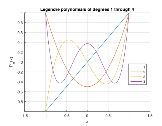
Figure 1: Legendre polynomial are plotted for orders $1,2,3,4.$

The following parametric model is considered for the temporal covariance function of the Fourier random coefficients $\{V_{l}\}$ of the log–intensity $\log(X_{t})$ in equation (3), with respect to the Legendre polynomial basis (see, e.g., [7];[24]):

$$B_{l}(t,s) = E[V_{l}(t)V_{l}(s)]=(1/2)\frac{(l+1)^{-2-|t-s|}}{(1+(t-s)^{2})^{\theta\beta(l)}}$$

$$\beta(l) = ((8/10)(l+1))/((l+1)^{2}+1)^{1/2},\ l\geq 0,\ t,s\in\mathcal{T}.$$ (15)

Thus, as given in Theorems 4 in [22], from (15), the kernel family $\{r_{t-s}(\cdot,\cdot),\ t,s\in\mathcal{T}\}$ associated with the cross-covariance operator family $\{R_{t-s}=E[\log(X_{t})\otimes\log(X_{s})],\ t,s\in\mathcal{T}\}$ of the $L^{2}(\mathbb{S}_{2})$–valued log–intensity is given by:

$$r_{t-s}(\langle\mathbf{x},\mathbf{y}\rangle)=\sum_{l=0}^{\infty}B_{l}(t-s)\frac{2l+1}{4\pi}P_{l}(\langle\mathbf{x},\mathbf{y}\rangle),\ t,s\in\mathcal{T},\ \mathbf{x},\mathbf{y}\in\mathbb{S}_{2}.$$ (16)

Figure 2 displays the values of the Log–Gaussian intensity $\log(X_{t})$ in equation (3), having covariance kernel (16) for $\theta=1$ in (15), after truncating series expansion (3) at $M=5.$ In practice, model (15) is parametrically fitted by least–squares from a temporal $100\times 100$ regular grid, from the projection into the Legendre basis of the empirical cross–covariance operators of the data, whose functional values are approximated over a spherical regular grid of $225\times 225$ nodes.

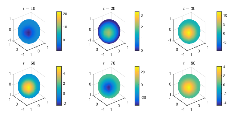
Figure 2: Log-intensity values on sphere for times $t=10,20,30,60,70,80.$

Shannon–entropy based distance $D^{S}_{q}$ in (9) is approximated by $\widehat{D}^{S}_{q}$ at Legendre scales $q=0,\dots,30,$ to measure the statistical distance between the two–order product densities of the generated spherical Log–Gaussian Cox process, and the spherical homogeneous Poisson process over the interval $[0,10].$ The estimate $\widehat{D}^{S}_{q}$ is computed by applying Monte Carlo numerical integration, based on a sample of size $1000,$ and least–squares parametric five–degree polynomial fitting for interpolation and smoothing. Figure 3 below displays three plots representing the values of $\widehat{D}^{S}_{q},$ for three embedded spatial scale sets, i.e., for $q$–values: $q=0,1,2,3,4,5$ (left–hand side), $q=0,\dots,20$ (center) and $q=0,\dots,30$ (right–hand side). One can observe the positive values of the computed statistical distances at Legendre scales zero to four indicating clustering, while null values are displayed from scales five to thirty. Maximum distance or aggregation level is attained at Legendre scales zero to one, decreasing to zero distance through scales two to four, leading to a regular behavior at Legendre high frequencies ($q\in\{5,\dots,30\}$), i.e., complete randomness at small scale.

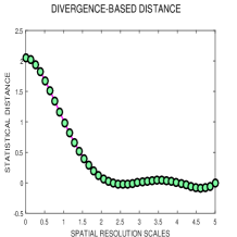
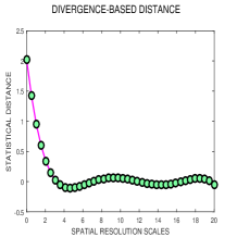
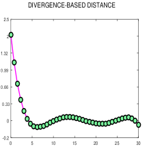
Figure 3: Statistical distance based on Ibragimov contrast function (9) between the two–order product densities of the generated spherical Log–Gaussian Cox process ($\theta=1$), and of spherical homogeneous Poisson process over the interval $[0,10],$ considering Legendre scales $q=0,1,2,3,4,5$ (left), $q=0,1,2,3,\dots,20$ (center), and $q=0,1,2,3,\dots,30$ (right), reflected at the horizontal axis.

Integral (9) defining $D_{q}^{S}(\rho^{(n)}_{q},\rho_{q}^{n})$ is computed for $n=3$ by applying trapezoidal rule. As expected, the classification results displayed in Figure 3 for the case of $n=2$ are supported in the Log–Gaussian case for $n=3,$ over all Legendre scales tested (see Figure 4).

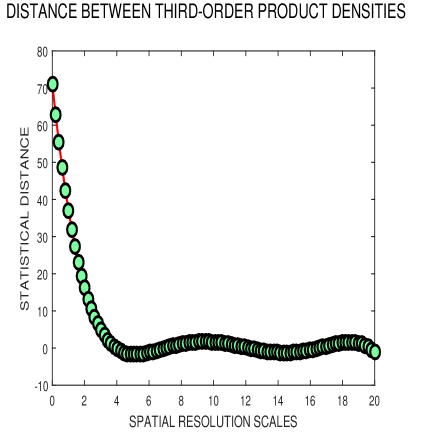
Figure 4: Shannon–based distance (9) for comparing third–order product densities of spherical homogeneous Poisson process, and spherical Log-Gaussian Cox process over the interval $[0,10].$ Here, the random coefficients $V_{n}$ in series expansion (3) have covariance function (15) with $\theta=1.$

Distance $D_{q,h}^{R}$ in (10) is now approximated by $\widehat{D}^{R}_{q,h},$ computed by applying Monte Carlo numerical integration and five degree polynomial least–squares smoothing. A similar pattern to the one displayed at the left–hand–side plot in Figure 3 is observed for the computed estimates of Rényi–entropy based distances $\widehat{D}_{q,h}^{R}$ of different integer and fractional orders $h,$ considering Legendre scales $q=1,2,3,4,5.$ Such empirical distances provide additional information about the clustering index in the spatiotemporal point pattern. Figures 5 and 6 show such distances in the respective cases of short– and long– range dependence in time of the log–intensity, corresponding to the values $\theta=100$ and $\theta=1/100$ in equation (15).

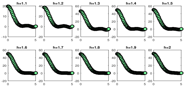
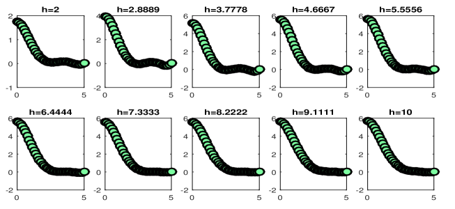
Figure 5: Weak–dependent case ($\theta=100$). Rényi distances $D_{q,h}^{R},$ $q=1,2,3,4,5$ (horizontal axis), and $h\in(1,10).$

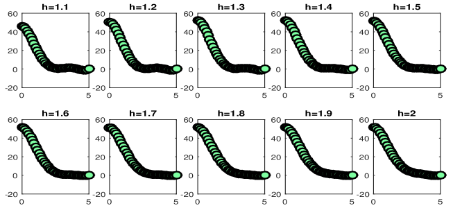
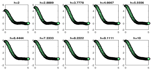
Figure 6: Strong–dependent case ($\theta=1/100$). Rényi distances $D_{q,h}^{R},$ $q=1,2,3,4,5$ (horizontal axis), and $h\in(1,10).$

All computed statistical distances reflect the same pattern with respect to Legendre scales (horizontal axis), indicating regularity at Legendre scales larger or equal than five ($q\geq 5$), and clustering at Legendre scales zero to four ($q=0,1,2,3,4$). Spherical scales $q=0$ and $q=1$ display the largest aggregation index CI${}_{h}=exp(D_{q,h}^{R}),$ under the three dependence models ($\theta=1,100,1/100$) for all computed statistical distances. For this particular scenario where Log-Gaussian intensities are considered, the log–intensity dependence range (reflected in parameter $\theta$), and the statistical distance chosen (reflected in parameter $h$) only affect the magnitude of the distances computed at the first spherical scales. Specifically, the clustering level, measured by the clustering index CI${}_{h},$ increases when the dependence range becomes larger at these first scales ($q=0,1,2$) around the integer values $h=1$ and $h=2$ of parameter $h.$

Large and small scale point pattern classification is here performed from Monte Carlo estimates $\widehat{K}_{q},$ $q=0,\dots,30,$ of functions $K_{q},$ $q=0,\dots,30,$ respectively. The pointwise differences $\widehat{K}_{q}-K_{\mbox{\small Pois}},$ $q=0,\dots,30,$ with $K_{\mbox{\small Pois}}$ denoting as before the theoretical $K$ function of spatiotemporal spherical Poisson process, are plotted in Figures 7–9, respectively corresponding to the long–, intermediate– and short–range dependence cases of the log–intensity, for Legendre scales $q=1,7,13,19,25.$ These functions are evaluated at the angular distances $\{\theta_{i},i=1,\dots,14\}=\left\{0,0.2244,0.4488,0.6732,0.8976,\right.$ $\left.1.1220,1.3464,1.5708,1.7952,2.0196,2.2440,2.4684,2.6928,2.9172,3.1416\right\},$in the interval $[0,\pi],$ and at the temporal distances $\left\{t_{i},i=1,\dots,14\right\}=$ $\left\{0,0.7143,1.4286,2.1429,2.8571,3.5714,4.2857,5.0000,5.7143,6.4286,7.1429,\right.$ $\left.7.8571,8.5714,9.2857,10.0000\right\},$ in the interval $[0,10].$

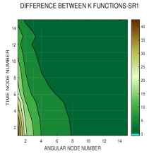
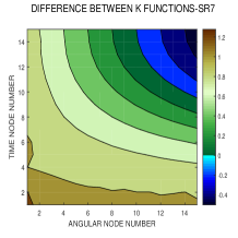
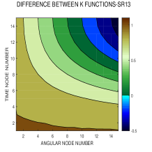
Figure 7: Long–range dependence (LRD) Gaussian log–intensity. Contour plots of pointwise values of empirical difference $\widehat{K}_{q}-K_{\mbox{Pois}},$ for $q=1,7,13$ (top) and for $19,25$ (bottom). The generated spherical Log-Gaussian Cox process over the time interval $[0,10]$ has Legendre Fourier coefficients having covariance function (15) with $\theta=1/100$ (LRD).

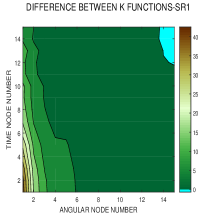
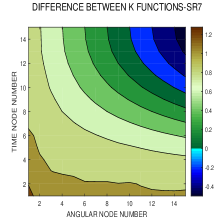
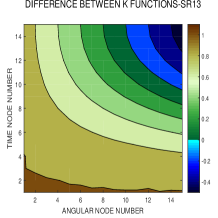
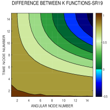
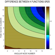
Figure 8: Intermediate dependence range in the Gaussian log–intensity. Contour plots of pointwise values of empirical difference $\widehat{K}_{q}-K_{\mbox{Pois}},$ for $q=1,7,13$ (top) and for $19,25$ (bottom). The generated spherical Log-Gaussian Cox process over the time interval $[0,10]$ has Legendre Fourier coefficients having covariance function (15) with $\theta=1.$

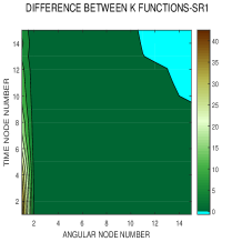
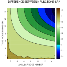
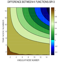
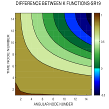
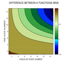
Figure 9: Short–range dependence in the Gaussian log–intensity. Contour plots of pointwise values of empirical difference $\widehat{K}_{q}-K_{\mbox{Pois}},$ for $q=1,7,13$ (top) and for $19,25$ (bottom). The generated spherical Log-Gaussian Cox process over the time interval $[0,10]$ has Legendre Fourier coefficients having covariance function (15) with $\theta=100.$

Figures 7–9 show that, for all log–intensity dependence ranges, $\widehat{K}_{q}-K_{\mbox{{\small Pois}}}$ values are decreasing when the Legendre spatial scale $q$ increases, going to zero when $q$ goes to infinity. Hence, for large values of $q,$ it can be observed that $\widehat{K}_{q}$ is pointwise approximating function $K_{\mbox{{\small Pois}}}$ (pointwise differences less than one for any temporal $t$ and angular $\theta$ distance values), supporting again the computational results showed in Figures 3–6. Thus, regularity of spatiotemporal point patterns at high Legendre frequencies ($q$ large) is observed, while aggregation or clustering is displayed at low Legendre frequencies ($q$ small), where bigger differences are induced by the log–intensity dependence range, i.e., larger positive pointwise discrepancies (stronger departure from regularity) are observed when the dependence range increases (see, e.g., contour plots at the top-left in Figures 7, 8 and 9).

Summarizing, for small arguments $t$ and $\theta$ of $\widehat{K}_{q}-K_{\mbox{{\small Pois}}}$ functions, more pronounced differences are observed through Legendre scales, while a regular behavior is observed for large values of $t$ and $\theta,$ i.e., null values of $\widehat{K}_{q}-K_{\mbox{{\small Pois}}}$ functions for every $q>1.$ For $q=1,$ positive pointwise discrepancies between $K$–functions hold for all ranges analyzed of $t$ and $\theta.$ One can also observe that for this $q=1$ value the effect of the dependence range of the Gaussian log–intensity is stronger, increasing positive discrepancies between $K$ functions compared, for all arguments $t$ and $\theta.$ For the rest of scales ($q\geq 2$), the effect of the dependence range is more pronounced at small values of $t$ and $\theta.$

6 Final comments

Under stationarity in time and isotropy in space, the present paper performs a statistical analysis of point patterns on a connected and compact two–point homogeneous space. Specifically, this analysis is based on Cox processes whose log–intensity (log–risk process) is Gaussian or belongs to the class of second–order mean–square continuous elliptically contoured random fields on a manifold (see, e.g., [22]). In the Gaussian case, a countable family of independent stationary centered Gaussian processes defines the time–varying discrete Jacobi polynomial transform of the log–intensity spatiotemporal random field. The $n$–order product density then admits an expression in terms of the infinite–product of $n$–order product densities corresponding to different Jacobi polynomial scales.

The simulation study undertaken is based on Monte Carlo numerical integration and least–squares parametric polynomial curve fitting, allowing the implementation of the proposed point pattern analysis, based on empirical statistical distances and $K$–functions, in terms of the time–varying discrete Legendre polynomial transform. By exploiting the isometry properties with the sphere, the numerical results derived in this simulation study are extended to the case of Log–Gaussian Cox processes on a connected and compact two point homogeneous space evolving time. Thus, one can conclude for the wider introduced family of Log–Gaussian Cox processes, the regular behavior (complete randomness) of the point process at large scales in the manifold. While aggregation or clustering is displayed at small scale in the manifold. This Jacobi low– and high– frequency analysis is achieved at temporal and manifold micro–scale level of the point pattern, by measuring the statistical distance between the $n$–order product densities of the analyzed point process, at different Jacobi polynomial scales, and the $n$–order product density of homogeneous Poisson process on the manifold over a time interval. Different statistical distances are tested within the Shannon– and Rényi–entropy based distances. The last ones providing a micro–scale aggregation (or clustering) index of the point pattern depending on Jacobi scale. The effect of the temporal dependence range of the log–risk process is more pronounced at low frequencies of discrete Jacobi polynomial transform. Particularly, the Rényi–based micro–scale aggregation index increases when the temporal dependence range of the log–intensity increases at low Jacobi frequencies. While the effect of the temporal dependence range asymptotically disappears at high frequencies of the discrete Jacobi polynomial transform. The analysis of point patterns in terms of the associated countable family of $K$–functions, arising from discrete Jacobi polynomial transform, also supports the conclusions of the micro–scale analysis based on statistical distances between $n$–order product densities. Particularly, at low discrete frequencies (large scale), stronger differences between complete randomness and scale–dependent $K$–functions of the analyzed point pattern are observed.

The statistical methodology proposed for analysis and multi–scale classification of point patterns on a manifold over time, in the context of connected and compact two–point homogeneous spaces, within the framework of Cox processes, will be extended to the case of multifractal spherical log–risk processes in a subsequent paper (see, e.g., [21]) . Finally, we remark that the presented approach is applicable to further families of point processes, including the family of determinantal point process on a manifold evolving time (see, e.g., [25] and [26] for the spatial spherical case).

Acknowledgements This work has been supported in part by projects MCIN/ AEI/PGC2018-099549-B-I00, and CEX2020-001105-M MCIN/ AEI/10.13039/501100011033).

References

References

- [1] Alegría A, Cuevas–Pacheco F (2020) Karhunen–Loéve expansions for axially symmetric Gaussian processes: modelling strategies and approximations. Stoch Environ Res Risk Assess 34:1953–1965
- [2] Andrews GE, Askey R, Roy R (1999) Special Functions. Encyclopedia of Mathematics and its Applications. Vol. 71. Cambridge University Press, Cambridge
- [3] Anh VV, Broadbridge P, Olenko A, Wang YG (2018) On approximation for fractional stochastic partial differential equations on the sphere. Stoch Environ Res Risk Assess 32:2585–2603
- [4] Baddeley A, Gregori P, Mateu J, Stoica R, Stoyan D (2006) Case Studies in Spatial Point Process Modeling. Springer, New York
- [5] Besag J, York J, Molié A (1991) Bayesian image restoration with two applications in spatial statistics. Ann Inst Stat Math 43:1–59
- [6] Caponera A (2021) SPHARMA approximations for stationary functional time series in the sphere. Stat Infer Stoch Proc 24:609–634
- [7] Caponera A, Marinucci D (2021) Asymptotics for spherical functional autoregressions. Ann Stat 49:346–369
- [8] Caponera A, Durastanti C, Vidotto A (2021) LASSO estimation for spherical autoregressive processes. Stoch Process Their Appl 137:167–199
- [9] Cugliari J (2011) Prévision non paramétrique de processus á valeurs fonctionnelles. Application á la consommation d’électricité, University of Paris-Sud 11, PhD. Thesis, 2011. https://tel. archives-ouvertes.fr/tel-00647334
- [10] Cugliari J (2013) Conditional autoregressive Hilbertian processes. arXiv:1302.3488
- [11] Diggle PJ (2013) Statistical Analysis of Spatial and Spatio-Temporal Point Patterns. Taylor & Francis, Boca Raton
- [12] Da Prato G, Zabczyk J (2002) Second Order Partial Differential Equations in Hilbert Spaces. London Mathematical Society Lecture Note Series. 293. Cambridge University Press, Cambridge
- [13] Diggle PJ, Kaimi I, Abellana R (2010) Partial-likelihood analysis of spatio-temporal point-process data. Biometrics 66:347–354
- [14] Emery X, Porcu E (2019) Simulating isotropic vector–valued Gaussian random fields on the sphere through finite harmonic approximations. Stoch Environ Res Risk Assess 33:1659–1667
- [15] Frías MP, Torres–Signes A, Ruiz–Medina MD, Mateu J (2022) Spatial Cox processes in an infinite–dimensional framework. Test 31:175–203
- [16] Goncalves FB, Gamerman D (2018) Exact Bayesian inference in spatio-temporal Cox processes driven by multivariate Gaussian processes. J R Statist Soc B 80:157–175
- [17] Guan Y (2006) A composite likelihood approach in fitting spatial point process models. J Am Statist Ass 101:1502–1512
- [18] Guillas S (2002) Doubly stochastic Hilbertian processes. J Appl Probab 39:566–580
- [19] Illian J, Penttinen A, Stoyan H, Stoyan D (2008) Statistical Analysis and Modelling of Spatial Point Patterns. John Wiley & Sons, New York
- [20] Khan, MI, Saha, R (2021) Isotropy statistics of CMB hot and cold spots. arXiv:2111.05886.
- [21] Leonenko NN, Nanayakkara R, Olenko A (2021) Analysis of spherical monofractal and multifractal random fields. Stoch Environ Res Risk Assess 35:681–701
- [22] Ma C, Malyarenko A (2020) Time varying isotropic vector random fields on compact two points homogeneous spaces. J Theor Probab 33:319–339
- [23] Marinucci D, Peccati G (2011) Random fields on the Sphere. Representation, Limit Theorems and Cosmological Applications. London Mathematical Society Lecture Note Series 389. Cambridge University Press, Cambridge
- [24] Marinucci D, Rossi M, Vidotto A (2020) Non-universal fluctuations of the empirical measure for isotropic stationary fields on Ann Appl Probab 31:2311–2349
- [25] Møller J, Nielsen M, Porcu E, Rubak E (2018) Determinantal point processes on the sphere. Bernoulli 24:1171–1201
- [26] Møller J, Rubak E (2016) Functional summary statistics for point processes on the sphere with an application to determinantal point processes. Spat Stat 18:4–23
- [27] Robeson SM, Li A, Huang C (2014) Point-pattern analysis on the sphere. Spat Stat 10:76–86
- [28] Ruiz–Medina MD, Espejo RM, Ugarte MD, Militino A F (2014) Functional time series analysis of spatio-temporal epidemiological data. Stoch Environ Res Risk Assess 28:943–954
- [29] Sadr, AV, Movahed, SMS (2021) Clustering of local extrema in Planck CMB maps. Monthly Notices of the Royal Astronomical Society 503:815–829.
- [30] Torres–Signes A, Frías MP, Mateu J, Ruiz–Medina MD (2021) A spatial functional count model for heterogeneity analysis in time. Stoch Environ Res Risk Assess 35:1825–-1849. https://doi.org/10.1007/s00477-020-01951-5
- [31] Torres-Signes A, Frías MP, Ruiz-Medina MD (2021) COVID-19 mortality analysis from soft-data multivariate curve regression and machine learning. Stoch Environ Res Risk Assess 35: 2659–-2678. https://doi.org/10.1007/s00477-021-02021-0
- [32] Ugarte MD, Goicoa T, Ibáñez B, Militino AF (2009) Evaluating the performance of spatio–temporal Bayesian models in disease mapping. Environmetrics 20:647–665
- [33] Ugarte MD, Goicoa T, Militino AF (2010) Spatio–temporal modelling of mortality risks using penalized splines. Environmetrics 21:270–289
- [34] Ugarte MD, Goicoa T, Etxeberria J, Militino AF (2012) A P-spline ANOVA type model in space–time disease mapping. Stoch Environ Res Risk Assess 26:835–845