A general model-and-run solver for multistage robust discrete linear optimization

Abstract

The necessity to deal with uncertain data is a major challenge in decision making. Robust optimization emerged as one of the predominant paradigms to produce solutions that hedge against uncertainty. In order to obtain an even more realistic description of the underlying problem where the decision maker can react to newly disclosed information, multistage models can be used. However, due to their computational difficulty, multistage problems beyond two stages have received less attention and are often only addressed using approximation rather than optimization schemes. Even less attention is paid to the consideration of decision-dependent uncertainty in a multistage setting.

We explore multistage robust optimization via quantified linear programs, which are linear programs with ordered variables that are either existentially or universally quantified. Building upon a (mostly) discrete setting where the uncertain parameters—the universally quantified variables—are only restricted by their bounds, we present an augmented version that allows stating the discrete uncertainty set via a linear constraint system that also can be affected by decision variables. We present a general search-based solution approach and introduce our solver Yasol that is able to deal with multistage robust linear discrete optimization problems, with final mixed-integer recourse actions and a discrete uncertainty set, which even can be decision-dependent. In doing so, we provide a convenient model-and-run approach, that can serve as baseline for computational experiments in the field of multistage robust optimization, providing optimal solutions for problems with an arbitrary number of decision stages.

1 Introduction

1.1 Motivation and Main Contribution

Neither for the complexity class nor for polynomial-time algorithms are known. The formal term polynomial time is usually translated to the more intuitive meaning fast or tractable. However, if researchers were to interpret hardness results as no-hope results and take the resulting intractability literally, the beauty of the MIP solver world would not exist. It has become obvious that sufficiently many instances of various -complete problems can be solved by single solvers and have even market relevance. Thus, technological progress and intensive research has been able to produce remarkable tools, which is why we should not be deterred from tackling even more (theoretically) hard problems algorithmically. The observed phenomenon is neither limited to -complete problems, nor to feasibility problems, but can quite smoothly be extended to -complete optimization problems. From search perspective the gap between and seems not necessarily larger than the gap between ¶ and .

To underline the intuitive statement above, we present the solver Yasol, which name—Yet another solver—is a little homage to some “Yet another …” unix programs and helpful apps of the 1990s. It is a tree search based solver for multistage robust linear optimization problems and it operates on an extension of mixed integer linear programs. The instances this solver can deal with are so called quantified integer linear programs (abbr. QIP) where continuous variables are permitted in the final decision stage, and even with an extension where interrelations between decision variables and the uncertainty set occur (abbr. QIP+). They can be introduced from different perspectives: On the one hand, QIP are extended mixed integer linear programs (MIP) where the variables are ordered explicitly and each variable is assigned a quantifier ($\exists$ or $\forall$), adding a multistage robust perspective to MIP. On the other hand, QIP can be viewed as an extension of quantified boolean formula (QBF), with additional objective function and further allowing general integer (and some continuous) variables and arbitrary linear constraints, rather than binary variables and clauses, adding the optimization perspective to a generalized QBF. Additionally, QIP can be viewed as a mathematical game between an existential and a universal player that—while having to obey a set of (linear) rules—try to maximize and minimize the same objective function, respectively. In the context of robust optimization QIP and its extensions provide a convenient framework for multistage robust optimization problems with discrete polyhedral and even decision-dependent uncertainty set.

Tackling QIP and QIP+ instances algorithmically has thrived on the pioneering work of the MIP, QBF and game tree search community: Optimality proofs and several ideas for finding solutions can be adapted from MIP and QBF solving, while relying on heuristic and algorithmic game tree search concepts. In this paper we describe how we can adapt the theoretical, heuristic and algorithmic findings and approaches from these various research fields and we present QIP and QIP+ specific results, which are then merged together to obtain an easily accessible model-and-run solver for a large variety of multistage robust optimization problems. Along this path, the contributions of this paper are as follows:

• We provide an in depth introduction and analysis of QIP and focus on the augmented version QIP+ that allows modeling of multistage robust optimization problems with decision-dependent uncertainty.

• We introduce our solver Yasol that is able to deal with multistage robust linear discrete optimization problems, with mixed-integer recourse actions only in the final decision stage and discrete uncertainty, which even can be decision-dependent.

• We present a general search based approach for such problems, which stands in contrast to the commonly used reformulation, decomposition and approximation techniques used in multistage optimization.

• We discuss enhanced solution techniques and give insight into specialized heuristics.

• Using the example of the multilevel critical node problem [BCLT21] we showcase that quantified programming provides a convenient and straightforward modeling framework and we demonstrate that our model-and-run solver serves as suitable baseline for multistage robust optimization problems.

After considering the related literature we introduce the concept of quantified programming and present an augmented version allowing decision-dependent uncertainty in Section 2. In Section 3 we introduce our solver and explain the underlying solution process. Further techniques integrated into the solution process are discussed in Section 4. Before we conclude, we show how quantified programs can be used to model the multilevel critical node problem [BCLT21] in Section 5 and demonstrate the performance of our solver on these instances in Section 6.

1.2 Related Work

Quantified Programming

Quantified constraint satisfaction problems have been studied since at least 1995 [GPS95]. In 2003, Subramani revived the idea of universal variables in constraint satisfaction problems and coined the term Quantified Linear Program (QLP) [Sub03]. His QLP did not have an objective function and the universal variables could only take values in their associated intervals. In the following year he extended this approach by integer variables and called them Quantified Integer Programs (QIPs) [Sub04]. Later Wolf and Lorenz added a linear objective function [LW15] and enhanced the problem to: “Does a solution exist and if yes which one is the best.” In [HELW16] the extension of QIP allowing a second constraint system restraining the universally quantified variables to a polytope was introduced. This was further extended to allow decision-dependent uncertainty sets in [HL19]. In both papers, polynomial time reductions are presented, linking the extensions closely to the originating QIP. In a computational study the strength of using QIP for robust discrete optimization problems was illustrated [GH21], being able to optimally solve problems with up to nine stages.

As we deal with a (mainly) discrete domain, there is a tight connection to the quantified boolean formula problem (QBF), which can be interpreted as a multistage robust satisfiability problem with only binary variables which are restricted via logical clauses. In particular as our solver uses an internal binary representation of discrete variables, many techniques known from solving QBF can be adapted to help during the search process. Within the last few years several new techniques for solving QBF were developed and enhanced, such as clause selection [JMS15b], clause elimination [HJL⁺15], quantified blocked clause elimination [LBB⁺15], counter example guide abstraction refinement [JKMSC16], dependency learning [PSS19a], long-distance $Q$-resolution [PSS19b] as well as several preprocessing [WRMB17, LE19] and even machine learning techniques [Jan18, LRSL19]. With the recent surge of new research a number of general solvers evolved and emerged [RT15, LE17, Ten19] within a vivid competitive environment [PS19, LSvG16]. It is noteworthy that also research on specific optimization settings within the QBF framework was conducted [IJMS16].

Multistage Robust Optimization

The notion of quantified variables, asking for a strategy that hedges against all possible realizations of universally quantified variables is closely linked to robust optimization problems. In [GH21] it was shown how quantified programming is directly linked to multistage robust optimization. Robust optimization problems are mathematical optimization problems with uncertain data, where a solution is sought that is immune to all realizations of the uncertain data within the anticipated uncertainty set [BTN02, GMT14]. A compact overview of prevailing uncertainty sets and robustness concepts can be found in [GYdH15, GS16]. By allowing wait-and-see variables, instead of demanding a single static solution, several robust two- and multi-stage approaches arose in recent years [BTGGN04, LLMS09, DI15, YGdH19], whereat the vast majority of research is restricted to a two-stage setting.

Besides directly tackling the robust counterpart, which is also referred to as deterministic equivalent program (DEP) [Wet74] or full expansion [JMS15a] in related areas, several other solution approaches for multistage problems exist. Dynamic programming techniques can be used [Sha11], but often suffer from the curse of dimensionality. Other solution methods include variations of Bender’s decomposition [TTE09] and Fourier–Motzkin elimination [ZDHS18]. Additionally, iterative splitting of the uncertainty set is used to solve robust multistage problems in [PdH16] and a partition-and-bound algorithm is presented in [BD16]. By considering specific robust counterparts a solution can be approximated and sometimes even guaranteed [BTGGN04, BTGS09, CZ09]. Furthermore, several approximation schemes based on (affine) decision rules can be found in the literature (e.g. [BIP10, KWG11, BG15, GKW19]).

In robust optimization it is frequently assumed that the occurring uncertainty is embedded in a predetermined uncertainty set, i.e. it is assumed to be exogenous. We use the term decision-dependent uncertainty for problems in which realizations of uncertain variables can be manipulated by decisions made by the planner. Others use the term endogenous uncertainty (e.g. [LG18, ZF20]) or terms like variable uncertainty (e.g. [P.14]) or adjustable uncertainty set [ZKG⁺17]. We refer to [Har20] for a more exhaustive discussion.

In the general context of optimization under uncertainty several solvers, modeling tools and software packages for robust optimization [GS11, Dun16, WM21] even with endogenous uncertainty [VJE20] as well as stochastic and distributionally robust optimization [CSX20] have been developed. Furthermore, for the special case of combinatorial three-stage fortification games a general exact solution framework was presented in [LLM⁺21]. The other mentioned solvers for robust optimization problems that can also cope with multistage settings, however, rely on approximation schemes—in particular decision rules—for adjustable variables and therefore cannot—in general—guarantee the optimality of the proposed solution. To the best of our knowledge, there exists no general solver that is able to solve problems within a multistage robust discrete linear optimization setting—let alone a setting with decision-dependent uncertainty—to optimality.

2 Problem Definition

This section deals with the mathematical object of interest. First we present the so called quantified linear program with minimax objective [LW15] and with integer variables, which builds the bridge to well known mathematical programming. This is structured in so called stages and is called QIP, where we additionally allow continuous variables in the last decision stage. The second problem statement, which we call QIP+, generalizes and extends the QIP problem, allowing decision-dependent and polyhedral uncertainty in the multistage discrete setting.

Throughout the paper we use the notation $[n]=\{1,\ldots,n\}$ to denote index sets. Furthermore, vectors are always written in bold font and the transpose sign for the scalar product between vectors is dropped for ease of notation.

2.1 The problem QIP

The main component of a QIP is a linear constraint system $A^{\exists}\boldsymbol{x}\leq\boldsymbol{b}^{\exists}$. Each variable is either existentially or universally quantified. An example may be

$$\exists x_{1}\in\{0,1\}\ \forall x_{2}\in\{0,1\}\ \exists x_{3}\in[-2,2]:\begin{pmatrix}-10&-4&2\\ -10&4&-2\\ 10&4&1\\ 10&-4&-1\end{pmatrix}\cdot\begin{pmatrix}x_{1}\\ x_{2}\\ x_{3}\end{pmatrix}\leq\begin{pmatrix}0\\ 4\\ 12\\ 8\end{pmatrix}$$

and the question to this instance is: ”Is there an $x_{1}$ such that for all $x_{2}$ there is an $x_{3}$ such that all constraints hold?”. Of course, the variables must have well-defined domains, and there may be sequences of variables of the same kind. Such a sequence of variables of one kind, either existential or universal variables, belong to the same so called variable block. A major restriction in this paper is that continuous variables may only occur in a final existential variable block. All other variables have to be integer with finite upper and lower bounds. Different than in conventional MIP, the quantifier alternations enforce a variable order that has to be considered.

Moreover, it is possible to incorporate an objective function. However, this objective has a minimax character, i.e. if an optimizer strives at large objective values, he has to consider a universal ’player’ minimizing over her domain. For our example it may look as follows:

$$\max_{x_{1}\in\{0,1\}}\left(x_{1}+\min_{x_{2}\in\{0,1\}}\left(+x_{2}+\max_{x_{3}\in[-2,2]}-x_{3}\right)\right)$$

Following the example above, a solution is no longer a vector of length three, but it is a tree of depth three that describes how to act and react with $x_{1}$ and $x_{3}$, depending on possible assignments of $x_{2}$. Such a tree-like solution is called a strategy. One possible solution strategy with minimax value $1$ is $x_{1}=0$, then—depending on the opponent’s move—either $x_{2}=0$ and $x_{3}=-2$ resulting in objective value $2$, or $x_{2}=1$ and $x_{3}=0$ with objective value $1$, as depicted in strategy 1 in Figure 1. The minimax-value $1$ of this strategy is defined via the objective value arising in the worst-case realization of the universally quantified variables, in this case $x_{2}=1$. Hence, not all strategies have the same minimax-value, and thus there is an optimization problem. E.g. the strategy 2 in Figure 1, which sets $x_{1}=1$ and then either $x_{2}=0$ and $x_{3}=2$, or $x_{2}=1$ and $x_{3}=-2$ has a worst-case objective value of $-1$ and therefore constitutes a worse strategy.

Figure 1: Two strategies with minimax values at each node.

Remark 1.

When depicting game trees or strategies we use square existential (MAX) nodes, circular universal (MIN) nodes, and rectangular leafs.

More formally, let $\boldsymbol{x}=(x_{1},\ldots,x_{n})^{\top}\in\mathbb{R}^{n}$ be a vector of $n$ (ordered) variables and $\boldsymbol{Q}\in\{\exists,\forall\}^{n}$ a quantification vector, assigning a quantifier to each variable. Every maximal consecutive subsequence in $\boldsymbol{Q}$, consisting of identical quantifiers, is called a quantifier block, where the quantifier of the $t$-th block is given by $Q^{(t)}\in\{\exists,\forall\}$. Let $T$ be the number of such blocks with $n_{t}\in\mathbb{N}$ being the number of variables in block $t$. The variable vector of block $t$ is referred to as variable block $\boldsymbol{x}^{(t)}$ and the domain for each inner variable block $t<T$ is given by the finite set $\mathcal{D}^{(t)}=\{\boldsymbol{x}^{(t)}\in\mathbb{Z}^{n_{t}}\mid\forall j\in[n_{t}]:\ell^{(t)}_{j}\leq x^{(t)}_{j}\leq u^{(t)}_{j}\}$ for $\boldsymbol{\ell}^{(t)},\boldsymbol{u}^{(t)}\in\mathbb{Z}^{n_{t}}$. In the final variable block also continuous variables are allowed, i.e. the corresponding domain is given by $\mathcal{D}^{(T)}=\{\boldsymbol{x}^{(T)}\in\mathbb{Z}^{n_{T}-\gamma}\times\mathbb{R}^{\gamma}\mid\forall j\in[s_{T}]:\ell^{(T)}_{j}\leq x^{(T)}_{j}\leq u^{(T)}_{j}\}$, with $\boldsymbol{\ell}^{(T)},\boldsymbol{u}^{(T)}\in\mathbb{R}^{n_{T}}$ and $\gamma\in[n_{T}]$ being the number of continuous variables. In case of a final universal variable block, i.e. $Q^{(T)}=\forall$, however, we demand $\gamma=0$. The domain of the entire variable vector is given by $\mathcal{D}=\{\boldsymbol{x}\in\mathbb{R}^{n}\mid\forall t\in[T]:\boldsymbol{x}^{(t)}\in\mathcal{D}^{(t)}\}$.

Definition 2 (Quantified Integer Linear Program (QIP)).

Let $A^{\exists}\in\mathbb{Q}^{m_{\exists}\times n}$ and $\boldsymbol{b}^{\exists}\in\mathbb{Q}^{m_{\exists}}$ for $m_{\exists}\in\mathbb{N}$. Let $\mathcal{D}$ and $\boldsymbol{Q}$ be given with $Q^{(1)}=Q^{(T)}=\exists$. Let $\boldsymbol{c}\in\mathbb{Q}^{n}$ be the vector of objective coefficients, for which $\boldsymbol{c}^{(t)}$ denotes the vector of coefficients belonging to the $t$-th variable block. The term $\boldsymbol{Q}\circ\boldsymbol{x}\in\mathcal{D}$ with the component-wise binding operator $\circ$ denotes the quantification sequence $Q^{(1)}\boldsymbol{x}^{(1)}\in\mathcal{D}^{(1)}\ \ldots\ Q^{(T)}\boldsymbol{x}^{(T)}\in\mathcal{D}^{(T)}$, such that every quantifier $Q^{(t)}$ binds the variables $\boldsymbol{x}^{(t)}$ of block $t$ ranging in their domain $\mathcal{D}^{(t)}$. We call

$$\textnormal{s.t.}\ \boldsymbol{Q}\circ\boldsymbol{x}\in\mathcal{D}:\ A^{\exists}\boldsymbol{x}\leq\boldsymbol{b}^{\exists}$$

a quantified integer linear program (QIP) with objective function (and final mixed-integer recourse).

Remark 3.

By allowing continuous variables in the final (existential) variable block we are in fact able to solve very specific quantified mixed integer programs.

2.2 Quantified Program with Interdependent Domains

Next, we present the QIP with interdependent domains (QIP+) [HL19, Har20]. This new mathematical object allows us to restrict the universal variables to a polytope or even allow this polytope to be changed by assignments of existentially quantified variables, making it suitable to model multistage robust optimization problems with polyhedral and even decision-dependent uncertainty.

In order to introduce this problem we first describe the QIP as a mathematical two-person zero-sum game and utilize this perspective to motivate the proposed extension. Imagine a game between a decision maker and an opponent. A play is represented by a variable vector $\boldsymbol{x}\in\mathcal{D}\subseteq\mathbb{Z}^{n}$, in which the variables are explicitly ordered and each variable belongs to either of the players, i.e. a vector of quantifiers $\boldsymbol{Q}\in\{\exists,\forall\}^{n}$ binds each variable. We refer to the decision maker as the existential player, as he will be in control of the existentially quantified variables and we are interested in the existence of a meaningful strategy. The opponent is called the universal player, as she controls the universally quantified variables and as we are not able to control her moves we have to anticipate all possible moves the opponent might be able to choose. Due to the ordering of the variables, variable blocks arise, which are given by maximal consecutive subsequences in $\boldsymbol{Q}$ consisting of identical quantifiers. We say a player makes move $\boldsymbol{x}^{(t)}=\boldsymbol{y}$, if she fixes the variable vector $\boldsymbol{x}^{(t)}$ of block $t$. In context of a game, the constraint system $A^{\exists}\boldsymbol{x}\leq\boldsymbol{b}^{\exists}$, together with the variable domains describe the game rules for the existential player.

Definition 4 (Game Tree).

The game tree $G=(V,E,e)$ of a QIP is an edge-labeled finite, rooted tree with a set of nodes $V=V_{\exists}\,\cup\,V_{\forall}\,\cup V_{L}$, unique root node $r\in V_{\exists}$, a set of edges $E$ and a vector of edge labels $e\in\mathbb{Q}^{|E|}$. The disjoint sets $V_{\exists}$, $V_{\forall}$ and $V_{L}$ contain existential decision nodes, universal decision nodes and leaf nodes, respectively. The level of a node $v\in V$ is the number of edges in the path from $r$ to $v$. Inner (non-leaf) nodes with the same level are either all existential decision nodes or all universal decision nodes. The $j$-th variable is represented by inner nodes with level $j-1$. Therefore, outgoing edges from a node $v\in V$ in level $j-1$ represent moves from $\mathcal{D}_{j}$ and the edge labels encode the corresponding variable assignments.

Remark 5.

Allowing continuous variables in the final existential variable block seems to contradict the use of a finite tree. However, as such variables are placed in the final block, we regard them as part of the leaf evaluation, and not as true decision variables: after all discrete variables have been assigned, a leaf is reached and the value of the leaf is the result of the remaining linear program.

In contrast to the standard QIP, where the universal player only has to adhere to the universal variable’s domains, now, each player gets an own rule book, given by two constraint systems $A^{\exists}\boldsymbol{x}\leq\boldsymbol{b}^{\exists}$ and $A^{\forall}\boldsymbol{x}\leq\boldsymbol{b}^{\forall}$. The first and foremost objective of each player is to prevent a violation of her respective constraint system, i.e. if a player is no longer able to ensure the satisfiability of her constraint system this player loses as there are no legal moves left. In particular, we call a move $\boldsymbol{x}^{(t)}=\boldsymbol{y}$ legal, if after setting $\boldsymbol{x}^{(i)}$ to $\boldsymbol{y}$ at least one solution of the current player’s constraint system exists, with respect to the given variable domains. If a play is completed and both constraint systems are fulfilled the payoff $\boldsymbol{c}\boldsymbol{x}$ is made by the universal player to the existential player. Therefore, the existential player aims at maximizing this payoff, while the universal player tries to minimize it. Overall this game can have three different endings: a) the existential player has no legal move left and the payoff is $-\infty$, b) the universal player has no legal move left and the existential player receives $\infty$, and c) the play ends with both constraint systems being fulfilled and $\boldsymbol{c}^{\top}\boldsymbol{x}$ is payed to the existential player. Note that a stalemate is impossible in this setting: As only legal moves are allowed, in every game position reached by legal moves, at least the constraint system of the previous player still has a solution. Only the degenerate case where both constraint systems do not have any solution from the start has to be excluded.

Let us now formally describe this problem. As before, a vector of $n$ variables $\boldsymbol{x}=(x_{1},\ldots,x_{n})^{\top}\in\mathbb{Q}^{n}$ and a quantification vector $\boldsymbol{Q}\in\{\exists,\forall\}^{n}$ assigning a quantifier to each variable, are the starting point. Let all terms and designations that relate to variables be the same as before. For now we prohibit the appearance of any continuous variables (cf. Section 2.3.3), in particular, $\mathcal{D}^{T}\subseteq\mathbb{Z}^{n}_{t}$.

Definition 6 (QIP with Interdependent Domains (QIP+)).

Let $m_{\exists}$, $m_{\forall}\in\mathbb{N}$ and let $A^{\exists}\in\mathbb{Q}^{m_{\exists}\times n}$, $\boldsymbol{b}^{\exists}\in\mathbb{Q}^{m_{\exists}}$ and $A^{\forall}\in\mathbb{Q}^{m_{\forall}\times n}$, $\boldsymbol{b}^{\forall}\in\mathbb{Q}^{m_{\forall}}$ be the left-hand side matrices and right-hand side vectors of the existential and universal constraint system, respectively. Let $\mathcal{D}$ and $\boldsymbol{Q}$ be given with $Q^{(1)}=\exists$ and $Q^{(T)}=\forall$. We demand $\{\boldsymbol{x}\in\mathcal{D}\mid A^{\forall}\boldsymbol{x}\leq\boldsymbol{b}^{\forall}\}\neq\emptyset$. The set of legal assignments of variable block $t$ (dependent on the assignment of previous variable blocks) $\mathcal{F}^{(t)}(\tilde{\boldsymbol{x}}^{(1)},\ldots,\tilde{\boldsymbol{x}}^{(t-1)})$ is given by

i.e. after assigning the variables of block $t$ there still must exist an assignment of $\boldsymbol{x}$ such that the system of the player in turn $Q^{(t)}\in\{\exists,\forall\}$ is fulfilled.

The vector of objective coefficients is given by $\boldsymbol{c}\in\mathbb{Q}^{n}$, where $\boldsymbol{c}^{(t)}$ denotes the vector of coefficients belonging to variable block $t$. We call

$$\textnormal{s.t.}\ \exists\boldsymbol{x}^{(1)}\in\mathcal{F}^{(1)}\ \forall\boldsymbol{x}^{(2)}\in\mathcal{F}^{(2)}\ \exists\boldsymbol{x}^{(3)}\in\mathcal{F}^{(3)}\ldots\ \forall\boldsymbol{x}^{(T)}\in\mathcal{F}^{(T)}:\ A^{\exists}\boldsymbol{x}\leq\boldsymbol{b}^{\exists}$$ (1)

a quantified integer linear program with interdependent domains (QIP+).

Observation 7.

Checking whether a universal variable assignment $\hat{\boldsymbol{x}}^{(t)}$ is legal, i.e. an element of $\mathcal{F}^{(t)}$, can be done by checking the feasibility of the IP $A^{\forall}\boldsymbol{x}\leq\boldsymbol{b}^{\forall}$ arising from fixing the variables of previous blocks accordingly, fixing $\boldsymbol{x}^{(t)}=\hat{\boldsymbol{x}}^{(t)}$ and demanding compliance with the general domain $\mathcal{D}$. For existential variable assignments the same process can be carried out for $A^{\exists}\boldsymbol{x}\leq\boldsymbol{b}^{\exists}$. We call this aspect the “no-suicide-rule”, as neither player is allowed to actively perform a move that results in an irreversible violation of her constraint system.

Definition 8 ((Winning) Existential Strategy).

A strategy (for the assignment of existential variables) $S=(V^{\prime},E^{\prime},e^{\prime})$ is a subtree of a game tree G = (V,E, e). $V^{\prime}$ contains the unique root node $r$, each node $v_{\exists}\in V^{\prime}\cap V_{\exists}$ has exactly one child in $S$ unless the set of legal moves at this node is empty. Each node $v_{\forall}\in V^{\prime}\cap V_{\forall}$ has as many children in $S$ as there are legal moves at this node. A strategy is called a winning strategy for the existential player, if $A^{\exists}\boldsymbol{x}_{v}\leq\boldsymbol{b}^{\exists}$ at each leaf $v$ representing a full game $\boldsymbol{x}_{v}\in\mathcal{D}$ and if all nodes in $V^{\prime}$ without outgoing edges are universal nodes.

Similar to a standard QIP, the solution of a QIP+ is a strategy in the game-tree search sense. The difference to the solution of a QIP is that a path in a QIP+ strategy not necessarily needs to reach a leaf of the game tree: If no legal variable assignment remains for the existential or universal player, a terminal node is reached, with extended minimax value $-\infty$ or $+\infty$, respectively. If there is more than one solution, the objective function aims for a certain (the “best”) one, whereat the value of a strategy is defined via the worst-case payoff at its terminal nodes (see Stockman’s Theorem [PdB01]). The play $\tilde{\boldsymbol{x}}$ resulting in this leaf is called the principal variation (PV) [CM83], which is the sequence of variable assignments being chosen during optimal play by both players.

Definition 9 (Extended Minimax Value).

Given the game tree $G=(V,E)$ of a QIP+. For any leaf $\ell\in V_{L}$ and the variable assignment $\boldsymbol{x}_{\ell}$ associated with this leaf the weighting function

$$w(\ell)=\begin{cases}c^{\top}x_{v}&\text{, $A^{\exists}\boldsymbol{x}_{\ell}\leq\boldsymbol{b}^{\exists}$ and $A^{\forall}\boldsymbol{x}_{\ell}\leq\boldsymbol{b}^{\forall}$ }\\ -\infty&\text{, $A^{\exists}\boldsymbol{x}_{\ell}\not\leq\boldsymbol{b}^{\exists}$ and $A^{\forall}\boldsymbol{x}_{\ell}\leq\boldsymbol{b}^{\forall}$ }\\ +\infty&\text{, $A^{\exists}\boldsymbol{x}_{\ell}\leq\boldsymbol{b}^{\exists}$ and $A^{\forall}\boldsymbol{x}_{\ell}\not\leq\boldsymbol{b}^{\forall}$ }\\ \pm\infty&\text{, $A^{\exists}\boldsymbol{x}_{\ell}\not\leq\boldsymbol{b}^{\exists}$ and $A^{\forall}\boldsymbol{x}_{\ell}\not\leq\boldsymbol{b}^{\forall}$}\end{cases}$$

determines the objective value of play $\boldsymbol{x}_{\ell}$, with $\pm\infty$ symbolizing an unknown outcome. For any node $v\in V$ the extended minimax value is defined recursively by

with the set $V_{\pm\infty}$, given by

$$V_{\pm\infty}=\{v\in V\setminus V_{L}\mid\forall v^{\prime}\in V:(v,v^{\prime})\in E\Rightarrow minimax_{e}(v^{\prime})=\pm\infty\}\,.$$ (2)

The nodes in set $V_{\pm\infty}$ represent partial variable assignments after which neither constraint system can be fulfilled. Thus, it contains nodes that cannot be reached via legal variable assignments, but note that $V_{\pm\infty}$ does not contain all nodes resulting from illegal moves. Having this extended minimax value at hand it becomes apparent that an adapted minimax algorithm can be applied to solve QIP+ instances. For a more detailed discussion of the game-tree representation we refer to [Har20].

Example 10.

Let $\boldsymbol{c}=(1,1,2)^{\top}$, $\boldsymbol{Q}=(\exists,\forall,\forall)$, $\mathcal{L}_{1}=\{1,2,3\}$ and $\mathcal{L}_{2}=\mathcal{L}_{3}=\{0,1\}$ and the two constraint systems given as follows:

$$A^{\exists}\boldsymbol{x}\leq\boldsymbol{b}^{\exists}:\quad\begin{array}[]{rcrcrcl}x_{1}&+&x_{2}&+&x_{3}&\leq&3\\ 2x_{1}&-&3x_{2}&&&\leq&3\par\end{array}$$

$$A^{\forall}\boldsymbol{x}\leq\boldsymbol{b}^{\forall}:\quad\begin{array}[]{rcrcrcl}-x_{1}&+&2x_{2}&+&x_{3}&\geq&0\end{array}$$

The game tree of this instance is give in Figure 2.

Figure 2: Game tree for the example instance. Illegal moves are indicated as dotted lines. The optimal winning strategy is indicated by thicker arrows.

The values at the leaves are assigned using the weighting function $w(v)$. The value of inner nodes were received by applying the extended minimax value. Hence, node values show the value according to optimal play starting from this node, whereat $\pm\infty$ denotes an illegal game situation that cannot occur during legal play. In the first existential stage $\mathcal{F}^{(1)}=\{1,2\}$ and in particular, $3\not\in\mathcal{F}^{(1)}$ since the existential constraint system can no longer be fulfilled for $x_{3}=3$. This can also be seen by looking at the leaves in the subtree beneath the decision $x_{1}=3$, wich all have the value $-\infty$ or $\pm\infty$. Note that if $x_{1}=2$ the universal variable $x_{2}$ cannot be set to $0$, since a violation of the universal system would become inevitable. In particular, $\mathcal{F}^{(2)}(x_{1}=2)=\{(1,0),(1,1)\}$. Furthermore, even though the extended minimax value of the node resulting from setting $x_{1}=2$ is $-\infty$ this move itself is not illegal; it only results in a game situation where no winning strategy for the existential player exists. Thus, even though $x_{1}=2$ is a bad move, it is still legal. The optimal course of play (the principal variation) is $x_{1}=1$, $x_{2}=1$, $x_{3}=0$ with objective value $\boldsymbol{c}\boldsymbol{x}=2$.

2.3 A closer look at the QIP+

2.3.1 The no-suicide-rule

One crucial point to motivate and explain the QIP+ is the no-suicide-rule. We use a small, rather degenerated, example in Table 1 with all binary variables, in order to show why it is noteworthy at all.

Table 1: A simple example for two constraint systems.

The existential constraint system consists of inequality (LABEL:eq::1) and equality (LABEL:eq::2) and the universal constraint system contains inequalities (LABEL:eq::3) and (LABEL:eq::4). An (illegal) line of play may be this:

$$x_{0}=0\rightarrow y_{0}=0\rightarrow x_{1}=1\rightarrow y_{1}=0\rightarrow x_{2}=0$$

Both systems are violated and the question is: what is the result? The solely symbolic value $\pm\infty$ describes this state by indicating the violation of both constraint systems, which cannot be placed in the ordered set $\{-\infty\}\cup\mathbb{R}\cup\{\infty\}$. However, the situation can be resolved when considering that both players where only allowed to take moves from their legal domain $\mathcal{F}$. Of course, when a player violates this rule, arbitrary nonsense can occur. Therefore, we have to detect who made the first illegal move.

Again, let us inspect Table 1. In principle, at the beginning of the game, both system are ”alive”, as binary assignments of the variables exist such that both systems for themselves can be fulfilled. Due to constraints (LABEL:eq::1) and (LABEL:eq::3) an assignment satisfying one system automatically violates the other system. Therefore no play can result in both systems being satisfied. Unclear is which player is first able to force the opponent’s set of legal moves to be empty. Setting $x_{0}=0$ is legal, as it does not affect the satisfiability of the existential constraint system. This forces the universal player to assign $y_{0}=0$, in particular, $\mathcal{F}^{(2)}((0))=\{0\}$. This assignment, however, results in the unsatisfiability of the existential constraint system, because constraint (LABEL:eq::2) can no longer be fulfilled: whatever both players will do next, no assignment of the forthcoming variables exist, that both adhere to the binary domain and fulfill $A^{\exists}\boldsymbol{x}\leq\boldsymbol{b}^{\exists}$. Thus, by definition, the existential player has no legal move and the result is $-\infty$. Going back to the initially presented illegal line of play: Setting $x_{1}=1$ was an illegal move and therefore should never have been executed. As the existential player cannot prevent the damning assignment $y_{0}=0$ no strategy exists to ensure the satisfaction of the existential constraint system, making this instance infeasible, indicated by the optimal outcome of $-\infty$.

The situation changes when inequality (LABEL:eq::4) is replaced by

$$y_{0}\geq x_{0}\,.$$

In this case, by setting $x_{0}=1$, the existential player can force the universal player to assign $y_{0}=1$. This preserves the satisfiability of the existential constraint system and $x_{1}=1$ is a legal move that immediately results in a violation of the universal constraint system. In this case, the result is $+\infty$.

2.3.2 Simply Restricted QIP+

In general, checking the legality of a universal (or existential) variable assignment, requires the feasibility of an IP, i.e. the solution of an -complete problem in every search node (see Definition 6). Intuitively, however, the resulting theoretical complexity appears unnatural and artificial: In terms of game playing determining the set of legal actions defined by the rules of the game is mostly a result of evaluating some if-then-else rules. Similarly in a robust optimization setting, identifying anticipated actions for the intangible adversary at each point in time intuitively should not be demanding at all.

We take advantage of this observation and introduce the simply restricted QIP+ for which the checking routine for the legality of a universal variable assignments can be simplified.

Definition 11 (Simply Restricted QIP+).

A QIP+ is called simply restricted, if the following holds: For any universal variable $i\in[n]$, $Q_{i}=\forall$, assignment $\tilde{x}_{i}\in\mathcal{D}_{i}$, and partial variable assignment $\hat{x}_{1}\in\mathcal{D}_{1},\ldots,\hat{x}_{i-1}\in\mathcal{D}_{i-1}$ it holds:

$$\tilde{x}_{i}\not\in\mathcal{F}_{i}(\hat{x}_{1},\ldots,\hat{x}_{i-1})\Rightarrow$$

$$\exists\,k\in\{1,\ldots,m_{\forall}\}:\sum_{j<i}A_{k,j}^{\forall}\hat{x}_{j}+A^{\forall}_{k,i}\tilde{x}_{i}+\sum_{j>i}\min_{x_{j}\in\mathcal{D}_{j}}A^{\forall}_{k,j}x_{j}\not\leq b^{\forall}_{k}\,.$$ (4)

Condition (4) ensures that a universal variable assignment $\tilde{x}_{i}\in\mathcal{D}_{i}$ is illegal, if there is a universal constraint that can no longer be fulfilled, even in the best case. Hence, rather than having to repeatedly solve the entire feasibility problem in order to check legality, it suffices to check the universal constraints separately in order to verify legality.

In [Har20], in order to be simply restricted, the additional requirement that at least one legal universal variable assignment has to be available at all times, even if the existential player played illegally. This requirement is no longer necessary as we will see in Section 3.4: situations during the search process where no legal universal assignment is left are handled separately by ensuring that this search node was reached via legal existential play.

It is noteworthy, that so far no automatic detection of simply restricted instances is implemented and the responsibility to detect it is handed over to the user. Some structural features where already analyzed in [Har20] and many instances arising from robust optimization with decision-dependent uncertainty exhibit this property.

2.3.3 Continuous Variables in the QIP+

In the definition of the QIP+ we demand a final universal variable block. Having the game interpretation in mind there is an easy explanation for this technicality: If the existential player would be in charge of the final move, the only things he would check are the satisfiability of the existential constraint system and the objective value. But what about the case that the final existential variable assignment results in a violation of the universal constraint system? This should result in the payoff $-\infty$. By demanding a final universal variable block this is implicitly dealt with, as now a violated universal constraint system implies an empty set of legal moves for the universal player, resulting in the payoff $\max_{x^{(T)}\in\emptyset}\boldsymbol{c}^{(T)}\boldsymbol{x}^{(T)}=-\infty$.

Furthermore, for QIP we allowed continuous variables in the final existential variable block. The definition of the QIP+ seems to prohibit this option as the final variable block needs to be universally quantified. However, there are two ways to bypass this in order to again allow a final existential variable block with continuous variables: a) Ensure that variables of the final existential variable block $T$ do not appear in the universal constraint system. This way the legal assignment of the previous universal variable block $T-1$ ensures that the universal constraint system is satisfied. b) When algorithmically dealing with such problems we can check the universal constraint system explicitly for every play (filled variable vector $\boldsymbol{x}$). This is equivalent to adding a final universally quantified dummy variable, which cannot alter the constraint system, but cannot be set legally if $A^{\forall}\boldsymbol{x}\leq\boldsymbol{b}^{\forall}$ no longer can be satisfied.

2.3.4 Distinction between variable bounds and constraints

For the basic QIP, modelling existential variable bounds via the domain $\mathcal{D}$ and via the existential constraint system is equivalent. For the QIP+, however, enforcing a bound via the variable domain is fundamentally different from adding a bound constraint in one of the constraint system. Consider the example with an existential variable $x_{1}$ and a universal variable $x_{2}$, both binary. The universal as well as the existential constraint system solely consists of the constraint $x_{1}+x_{2}\leq 1$ and let the objective function be the maximization of $x_{1}$. Having no objective function makes this instance clearly feasible, where setting $x_{1}=1$ is optimal. Assume now we want to ensure $x_{2}\geq 1$ as a rule for the universal player. If the constraint $x_{2}\geq 1$ is added to the universal constraint system, setting $x_{1}=1$ remains legal and in fact optimal, as it results in an empty legal domain for $x_{2}$. If, on the other hand, this is done by setting the lower bound of $x_{2}$ to $1$, setting $x_{1}$ to $1$ is no longer a legal move ($\mathcal{F}^{(1)}=\{0\}$), as with $x_{1}=1$ $\nexists x_{2}\in\mathcal{D}:x_{1}+x_{2}\leq 1$. In Figure 3 the corresponding game trees are illustrated where illegal variable assignments are dotted and each node holds its extended mininax values.

$\boldsymbol{Q}\circ\boldsymbol{x}$	$\exists x_{1}\in\{0,1\}\ \forall x_{2}\in\{0,1\}$		$\exists x_{1}\in\{0,1\}\ \forall x_{2}\in\{1\}$
$A^{\exists}\boldsymbol{x}\leq\boldsymbol{b}^{\exists}$	$x_{1}+x_{2}\leq 1$		$x_{1}+x_{2}\leq 1$
$A^{\forall}\boldsymbol{x}\leq\boldsymbol{b}^{\forall}$	$x_{1}+x_{2}\leq 1$		$x_{1}+x_{2}\leq 1$
	$x_{2}\geq 1$

Figure 3: Example Bounds vs. Constraints

Hence, the illustrated instances answer two different questions: One addresses the question, whether in the initially presented instance prematurely fixing $x_{2}=1$ results in a viable strategy for the universal player, while keeping $x_{2}=0$ a conceivable but rejected option. If, on the other hand, the domain $\mathcal{D}$ is altered, a fundamentally changed structure arises (see the changed game tree), deeming $x_{2}=0$ not part of any legal play and for that matter it can no longer serve as validation of the legality of $x_{1}=1$.

To complete the example, we point out, that adding $x_{2}\geq 1$ to both constraint systems once again results in $x_{1}=1$ being illegal. In fact, adding such constraints is equivalent to explicitly setting the bounds of the variable.

Therefore, when modeling such bound constraints, one first has to consider whether this bound constitutes a global restriction or a local instruction for one of the players.

2.3.5 Classification of the QIP+

The following special cases of the QIP+ illustrate the connection to other problem classes and show that the notion of legal moves and the “no-suicide-rule” is well embedded in our multistage domain.

1. If $T=1$ with $Q^{(1)}=\exists$ no universal variables exist and an MIP arises.

2. If there are no universal constraints, legal universal variable assignments only have to adhere to their initial domain $\mathcal{D}$. Legal existential variable assignments still must not result in a violation of the existential constraint system. The corresponding standard QIP, which ensures the fulfillment of the existential system at each leaf, results in the same optimal objective value.

3. A QBF arises, if $\mathcal{D}=\{0,1\}^{n}$, no universal constraint system and no objective function exists, and each constraint is a clause, i.e. $A^{\exists}\in\{-1,0,1\}^{m_{\exists}\times n}$ and $b^{\exists}_{i}=|\{j\in[n]\mid\ A^{\exists}_{i,j}=1\}|-1$ for each $\leq$-constraint $i\in\{1,\ldots,m_{\exists}\}$.

4. Assume universal variables are constrained by $A^{\forall}\boldsymbol{x}\leq\boldsymbol{b}^{\forall}$, but no existential variables occur in this system. Due to the condition $\{\boldsymbol{x}\in\mathcal{D}\mid A^{\forall}\boldsymbol{x}\leq\boldsymbol{b}^{\forall}\}\neq\emptyset$, there are always legal moves for the universal player and the optimal result cannot be $\pm\infty$. The resulting problem is similar to discrete robust optimization with polyhedral discrete uncertainty set and was investigated in the quantified programming setting in [HELW16, Har20, GH21].

5. The universal constraint system is modelled in a way that existential variables assignments only alter the set of legal universal variable assignments, but never result in irrevocable violation of the universal constraint system. In other decision-dependent domains this is explicitly mentioned as a task the modeler must deal with [LG18, FFZ21], or is ensured by allowing only specific structures [Pos14, NS18].

6. Assume, all constraints available in the universal constraint system are also present in the existential constraint system. Then the existential player has no chance of violating the universal constraint system as such move would be deemed illegal for him as well. In particular, due to $\{\boldsymbol{x}\in\mathcal{D}\mid A^{\forall}\boldsymbol{x}\leq\boldsymbol{b}^{\forall}\}\neq\emptyset$, legal play by the existential player always results in a satisfied universal constraint system.

Hence, QIP+ expands the modeling options of QIP, explicitly dealing with situations where the uncertainty set—the legal domain of universally quantified variables—can be restricted; even to be the empty set. In a game against nature [Pap85] this option is likely to be prevented by the modeler, as it seems implausible to be able to act as the decision maker in such a way that nature has no move left and surrenders. However, there are settings, where this option can come in handy, e.g. when the universal player represents a competitor.

Also note that the explicit reduction from QIP+ to QIP [HL19, Har20] illustrates that restricting the universal player also can be done implicitly within a standard QIP by sophisticated modelling techniques that penalize certain variable assignments, making them detrimental in the optimization context.

Our solver can deal with all of the above mentioned cases. In Section 6 we can show that for a problem with decision-dependent uncertainty we are able to keep up even with domain specific techniques.

3 The Solver and the Solution Process

3.1 The Solver Yasol

Yasol is a search based solver for quantified integer linear programs with interdependent domains and mixed-integer recourse in the final decision stage. In particular, it is able to deal with multistage optimization problems with polyhedral and decision-dependent uncertainty set and is available as open-source software.

The basic data structure of Yasol is a database of existential constraints, with an own memory management that allows to shrink the database in place when learnt constraints are not useful enough. Let us call this the primary constraint database. To solve relaxations, the whole instance is duplicated in the constraint system of an LP-solver. An abstract LP solver is used as an interface to the LP-solvers Cplex or CLP. Lets call this the LP constraint database.

The constraints in the primary database are organized in rows and a column supporting list keeps track which variables are contained in which constraints. The rows of the database and the columns of the supporting list keep additional information, where to find the variable, i.e. the column structure knows that a variable $x$ is in constraint $c$ at position $i$. Vice versa, the row knows where to find a variable in the supporting column structure.

Internally, general integer variables are first transformed to have the lower bound $0$ and are subsequently binarized. Therefore, upper bound constraints for such binarized variables are explicitly added to the existential as well as the universal constraint system creating an QIP+. The number of bits depends on the input, here it is of advantage that all variables must have upper and lower bounds on their domains a priori. There is an additional data structure which keeps track of bits of general integer variables. In this way, the integer information is kept and can be exploited.

As only binary variables are used for branching, the branching is not done symbolically in form of adding constraints to the system, but the variables can be assigned, i.e. temporarily set to $0$ or $1$. When a variable is set during the search process, it is carefully documented which consequences this has. Some constraints may be temporarily taken out of the constraint system and when the variable is un-assigned, the major datastructure will be in the same state as they were before. This allows to learn a new constraint after a conflict-analysis in such a way that the search process continues after learning as if the new constraint had been in the system from the beginning on.

On the LP-side, constraints are added in a greedy lazy manner in order to avoid simplex-computations on thousands of superfluous constraints. They are added and deleted during the tree search in depth-first-search manner, because the major algorithm, the Alpha-Beta algorithm works that way. Cutting planes like GMI or cover cuts are handled in the same way as normal constraints. However, the constraints of the primary database and of the LP are strictly seperated and usually cuts are not learnt into the primary database and vice versa.

3.2 Input and Output Format for the Solver

QIP+ instances have to adhere the following mild restrictions in order to be solvable with our solver:

• The final variable block has to be existential, i.e. $Q_{n}=\exists$ or rather $=Q^{(T)}=\exists$, which can be achieved by adding a single dummy variable.

• Variables with a continuous domain have to be part of a final existential variable block $T$. All other domains $\mathcal{D}^{(t)}$ for $t=1,\ldots,T-1$ have to be discrete.

• The domain $\mathcal{D}$ has to be bounded, i.e. for each variable a lower and upper bound is given.

• The uncertainty set, i.e. the domain of the universally quantified variables can either be boxed, polyhedral or decision-dependent, where for the latter two a linear universal constraint system $A^{\forall}\boldsymbol{x}\leq\boldsymbol{b}^{\forall}$ is used.

The QLP-file format extends the CPLEX LP-file format by adding the keywords ALL, EXISTS and ORDER, which enable the identification of universal and existential variables as well as the order of the variables, respectively. In order to allow constraints restricting the universally quantified variables, we further added the keyword UNCERTAINTY SUBJECT TO.

The output of our solver comprises of the optimal objective value, as well as the principal variation, which is the optimal path in the underlying strategy leading to this objective value. In particular, the first stage solution can be stated. We provide an XML formatted solution file, that also can hold the incumbent solution in case of exceeding the prespecified runtime. An example of the file formats is given in Appendix A.

3.3 Central Algorithm

In this section we present the central algorithm as briefly outlined in the proceedings [EHL⁺17]. In an intermediate step, we assume a standard QIP without universal constraints, before we consider the general algorithm for QIP+ in Section 3.4.

The heart of Yasol’s search engine is a customized Alpha-Beta algorithm as outlined in Algorithm 1 that is branching on binary variables. This extended Alpha-Beta algorithm walks through the search space recursively and fixes variables to $0$ or $1$ when going into depth or relaxes the fixations again when returning from a subtree. In the algorithm the decision level $d$, indicates the number of active decision nodes from the current search node $v$ to the root node, where implied unit-propagated variables are not counted.

Remark 12.

As continuous variables are only allowed in the very last stage they are not subject to branching and are assigned according to a call to the LP solver at a leaf.

Essentially, Algorithm 1 is an extension of the conventional Alpha-Beta algorithm [KM75] that develops if the lines 1 and 1 within Alg. 1 are deleted, and the lines 1 to 1 are replaced by Code Snippet 1.

1 if $x_{v}$ is existential variable then

       value := alphabeta(d+1, max(alpha, score), beta);

       // $value$ takes the minimax result from child node

      

else

       value := alphabeta(d+1, alpha, min( score, beta));

      

Snippet 1: Code Snippet of the Original Alpha-Beta Algorithm

The original Alpha-Beta algorithm is an improved minimax-search, and technically, a depth-first branch-and-bound procedure which deals with lower and upper bounds $\alpha$ and $\beta$. At each search node $v$, the window between $\alpha$ and $\beta$ indicates which minimax-values may be of interest at $v$. If the minimax-value at $v$ is below $\alpha$, $v$ will be irrelevant for the max-player. If it is above $\beta$, the node will be irrelevant for the min-player. Thus, as soon as the window at a node $v$ collapses, the subtree below $v$ is cut off. There have been many modifications and improvements, e.g. MTD(f) [PSPDB96a] and (nega)scout [Pea80, Rei83a], but most of them brought no benefits for our special situation. The most useful ones are addressed in the following in more detail.

The major advantage of the algorithm is that, in the best case, it determines the minimax-value of the root with only a minimum number of search nodes. This means, when the search breadth uniformly is $b$ and the search tree has uniform depth $d$, the best-case number of examined leafs is

$$\lfloor 2^{d/2}\rfloor+\lceil 2^{d/2}\rceil-1.$$

Figure 4: A strategy for the maximizing player on the left, a strategy for the minimizing player on the right, and both merged in the middle with the bold path from root to one of the leafs showing the principle variation.

This corresponds to the number of leafs for the maximizing player’s strategy plus the number of leafs for the minimizing player’s strategy minus that single leaf which both strategies have in common. The principal variation—the path from that common leaf to the root—shows a game under the assumption that both players play optimally. Detecting and verifying the principal variation is essential in order to obtain the objective value. In Figure 4 a small example illustrates this idea. How efficient the Alpha-Beta algorithm can traverse the tree, i.e. how many cutoffs can be applied by $\alpha$ and $\beta$ depends on the search node ordering. Having reasonable knowledge of which universal variable assignments are particularly vicious can massively boost the search process. Several heuristics exist to analyze and find such promising moves in a game tree search environment [AN77, WvdWvdHU04, Sch89, PSPdB96b] as well as in mixed integer programming [AKM05]. We utilize these ideas in a heuristic fashion to speed up our search process, where the so called killer-heuristic [AN77] turned out to be quite effective. Similarly, for existential nodes we can rely on heuristic branching rules [AKM05]. Furthermore, we can utilize the well-known concept of monotonicity [CSGG02] for both universal as well as existential variables, that allows us to omit certain subtrees a priori since solving the subtree of its sibling is guaranteed to yield the desired minimax value.

Observation 13.

Considering the special case of an MIP, the strategy for the existential player consists of only a single path in the tree. The counter strategy, however, the proof of optimality, consists of all paths in the tree. But from point of game tree search, the major challenge seems to be to find the exponentially large existential strategy, while for proving optimality we already ’stand on the shoulders of Giants’, being able to utilize cutting planes and conflict driven non-chronological backtracking from MIP, QBF and SAT solving. However, for finding existential strategies we are able to provide a fast heuristic approach to tackle the exponential growth (see Section 4.1).

One major extension in Algorithm 1 is the use of a relaxation (see Line 1), which is very well known in several optimization domains. This opens the opportunity to cut off parts of the search tree with the help of dual information, i.e. dual bounds or cutting planes for the original program, and additionally can be utilized in order to obtain useful branching information. Further details on how this relaxation is built are provided in Section 4.3.

The missing abilities of the standard Alpha-Beta to organize far jumps in the tree, and thus overcoming the strict chronological node order, is eliminated with the help of the code lines 1–1. The non-chronological back-jumping is either caused by constraint-learning like for QBF [ZM02] or in combination with Dual-Farkas certificates, Benders cuts and implication graphs as described in [Ach09a].

1 if $v$ is tree leaf then return objective value;

2 solve relaxation; extract branching variable $x_{v}$ of current block; determine search order 0/1 or 1/0 stored in $polarity$; maybe create some cuts;

3 $\textnormal{level\_finished($d$)}:=false$;

4 if $x_{v}$ is existential variable then score := $-\infty$;

else  score := $+\infty$;

5 for $i:=0$ to 1 do // examine two child nodes …

      6 assign($x_{v}$, $polarity$[$i$], …);

      7 repeat

            7.1 if level_finished($d$) then // leave dead-marked recursion levels

                   unassign($x_{v}$);

                   if $x_{v}$ is existential variable then  return score;

                   else  return $-\infty$;

                  

            

            7.2 if propagate(.) leads to no conflict then // cf. unit prop. [ZM02]

                  7.3 if $x_{v}$ is existential variable then

                        7.4 value := yAlphabeta($d$+1, max(alpha, score), beta);

                        7.5 if value $>$ score then score := value;

                        7.6 if score $\geq$ beta then break;

                        

                  7.7 else …analogously …;

                  

            else

                  7.9 addReasonCut(.); // add conflicting constraint (cf.[ZM02])

                  7.10 extract implied variable and target decision level $target\_d$;

                  7.11 for $k:=d$ down to target_d do

                        7.12 set $\textnormal{level\_finished($k$)}:=true$;

                        

                  7.12 if $x_{v}$ is existential variable then return score;

                  7.13 else  return $-\infty$;

                  

            

      until there is no backward implied variable;

      

      8 unassign($x_{v}$);

      

      9 if $v$ is existential node then

            9.29.1 if value $>$ score then score := value; // MAX node if score $\geq$ beta then return score;

      else

            9.49.3 if value $<$ score then score := value; // MIN node if score $\leq$ alpha then return score;

      

10 return score;

yAlphabeta(node $v$, decision level $d$, double alpha, double beta)

Algorithm 1 Core algorithm of the Yasol solver

yAlphabeta(node $v$, decision level $d$, double alpha, double beta)

Remark 14.

If the desired outcome of such a QIP search process is only feasible or infeasible, and if all LP-related code is eliminated, the procedure essentially degenerates to a variant of the QCDCL algorithm for QBF (cf. e.g [ZM02]).

As will be described in more detail in Section 4.3, free universal variables are heuristically fixed in the LP-relaxation by setting the respective variable bounds to $0$ or $1$. Let $\boldsymbol{x}_{a}$ be the part of the variable vector that is temporarily assigned by the depth-first-search and let $\boldsymbol{x}_{f}$ be the remaining $n_{f}\in[n]$ free variables. Then $\max\{\boldsymbol{c}_{a}\boldsymbol{x}_{a}+\boldsymbol{c}_{f}\boldsymbol{x}_{f}|A^{\exists}_{a}\boldsymbol{x}_{a}+A^{\exists}_{f}\boldsymbol{x}_{f}\leq\boldsymbol{b}^{\exists},\ \boldsymbol{x}_{f}\in[0,1]^{n_{f}}\}$ is the current LP-optimization problem. The LP-relaxation with these temporarily fixed variables gives a local upper bound on the objective value or, if the LP is already infeasible, a dual ray that is used to construct a new constraint for the original system of constraints. The dual of the LP-relaxation has the form min$\{\boldsymbol{\pi}(\boldsymbol{b}^{\exists}-A^{\exists}_{a}\boldsymbol{x}_{a})\mid A^{\exists}_{f}\boldsymbol{\pi}\geq\boldsymbol{c}_{f},\,\boldsymbol{\pi}\leq 0)\}$ and the Farkas lemma leads to the feasibility cut $\boldsymbol{\pi}(\boldsymbol{b}^{\exists}-A^{\exists}_{a}\boldsymbol{x}_{a})\leq 0$. This feasibility cut describes a subset of the fixed variables one of which must be changed from $1$ to $0$ or vice versa to reach feasible regions. The cut is added to the database of cuts on the QIP-database side. These cuts are not added to the LP. In favorable cases, the new cut proves that the search process can be abbreviated and continued several recursion levels above the current level. With some post-processing and conflict analysis [Ach07], these cuts are made more sparse and play an essential role for the QIP solution process.

How to process the new cuts is also closely related to the topic of how to propagate implied variables and how to organize backward implications, as SAT solvers or modern IP solvers like SCIP [Ach09a, Ach09b] do. The non-chronologic backtracking is realized with the help of lines 1 to 1 in Alg. 1. There is a loop around the Alpha-Beta procedure call which is repeated as long as backward implied variables occur deeper in the search tree. The procedure propagate(.) performs the implication of variables. In the context of boolean formulae, this process works identically with unit propagation. In more general constraints, further implications or bound propagations can be implied. The method addReasonCut(.) adds the output of a conflict analysis to the constraint database and thus implements the learning algorithm as used by modern IP-solvers as well. With the help of the original and the learnt constraints, the algorithm implicitly maintains an implication graph as described in [Ach07]

Example 15.

Figure 5: Search path tracing through a universal node $r$.

Let us inspect the situation in Fig 5. Let $u$ be some search node where a decision has been made to branch some binary variable $x_{u}$ to e.g. $1$. Then some implications may have arisen. Let the implications affect some $(x^{1}_{u},...,x^{k}_{u})$. Further, there have been other branching decisions at subsequent nodes. $r$ may even be a universal node, $w$ and $v$ some existential nodes. Now, assume a conflict arises at node $v$ and the conflict analysis (Line 1) shows that the polarity of the 0/1-decision variable $x_{v}$ can already be implied at node $u$. Then Algorithm 1 organizes a rapid rollback from node $v$ to $u$ via Line 1, by marking all nodes succeeded by $u$ as ’level_finished(.)’ in Lines 1 and 1, and by messaging ’$x_{v}$ is implied’ to node $u$. At node $u$, $x_{v}$ is now lined up to be implied in Line 1 and the branch below $u$ is re-searched with the implication sequence $(x^{1}_{u},...,x^{k}_{u},x_{v})$.

However, the situation may become more tricky. Let $z$ be the best-known minimax-value at the root, and $z^{*}_{v}$ the relaxation value at some node $v$, with $z<z^{*}_{v}\leq\alpha_{v}$. Then it is desirable to generate a local valid cut and a reasonable back-jump-level, as well. Again, let us inspect the tree clipping in Fig 5. Starting from the existential node $u$ with Alpha-Beta window $[\alpha,\infty]$, the universal node $r$ is reached. When the left branch of the existential node $w$ has been completed, node $v$ can be reached with the window $[\alpha^{\prime},\infty]$ with $\alpha^{\prime}>\alpha$. Then four cases can occur.

• $z^{*}_{v}\leq z$. This case is already covered as a conflict is learned and a backjump is conducted.

• $z^{*}_{v}>\alpha^{\prime}$. The regular search process proceeds.

• $z^{*}_{v}>z,z^{*}_{v}\leq\alpha$

• $z^{*}_{v}>\alpha,z^{*}_{v}\leq\alpha^{\prime}$. The latter two cases can be handled equivalently. Tightening the LP with the help of $\alpha^{\prime}$ leads to a cut. However, the search stack must be carefully examined in order to find out the best possible legal back-jump level. In fact, the algorithm may go upwards as long as existential nodes occur, or the universal nodes have the same $\alpha$ values as node $v$. So, in general, if the conflict analysis results in the insight ’… and this is implied already in node $u$’, the search can safely proceed in node $r$, but not in $u$, because the other branch of $r$ might still be relevant. However, if the current $\alpha$-value at $r$ is the same as $\alpha^{\prime}$ at node $v$, $r$ will never become relevant.

3.4 From QIP to QIP+

When adding a second constraint system $A^{\forall}\boldsymbol{x}\leq\boldsymbol{b}^{\forall}$ that restricts the universal variable assignments it no longer suffices to evaluate leafs, as it might be the case that both constraint systems are violated. Instead it has to be ensured that only legal variable assignments are performed during the search. However, checking the legality of a variable assignment requires the feasibilty and hence the solution of an IP. Therefore, instead of checking the legality of every variable assignment explicitly we show that it suffices to ensure that universal variable assignments have to be set in a legal manner at any time. Illegal existential variable assignments will be detected later on during the search, allowing us to omit finding a solution to the existential IP over and over again. Note that this procedure also could be done the other way around by ensuring the legality of existential assignments explicitly. However, the universal constraint system tends to be much smaller than the existential constraint system: $A^{\forall}\boldsymbol{x}\leq\boldsymbol{b}^{\forall}$ describes the uncertainty set, which in most common discrete applications is rather small, e.g. only containing budget constraints [BS04], cardinality constraints [GH21] or simple decision-dependent structures [BCLT21]. As already motivated in Section 2.3.2 (simply-restricted QIP+) in many use cases we additionally can benefit from a simple structure of the uncertainty set, where it is rather easy to see that a specific realization of the universal variable assignment is illegal.

The main idea why it suffices to ensure the legality of the universal variables is that this way we can be sure that a situation where both $A^{\exists}\boldsymbol{x}\leq\boldsymbol{b}^{\exists}$ and $A^{\forall}\boldsymbol{x}\leq\boldsymbol{b}^{\forall}$ are violated had to emerge from an illegal existential variable assignment, otherwise there must have been an illegal universal variable assignment, which then can no longer be the case. Due to the requirement $\{\boldsymbol{x}\in\mathcal{D}\mid A^{\forall}\boldsymbol{x}\leq\boldsymbol{b}^{\forall}\}\neq\emptyset$ at least one system still has a solution at the root node. In Algorithm 2 we extend Algorithm 1 to deal with general QIP+ by explicitly checking the legality of universal variable assignments (Line 2 in Algorithm 2). For the special case of a search node $v$ with $\mathcal{F}(v)\neq\emptyset$, i.e. a node without any legal successors, four cases have to be examined:

• A universal node $v_{\forall}$ is reached from a universal predecessor $w_{\forall}$ and $\mathcal{F}(v_{\forall})=\emptyset$, i.e. there is no legal universal variable assignment and the system $A^{\forall}\boldsymbol{x}\leq\boldsymbol{b}^{\forall}$ has no solution. With Line 2 in Algorithm 2 the search cannot not have traversed from $w_{\forall}$ to $v_{\forall}$ as it constitutes an illegal move.

• A universal node $v_{\forall}$ is reached from an existential predecessor $w_{\exists}$ and $\mathcal{F}(v_{\forall})=\emptyset$.

  • $A^{\exists}\boldsymbol{x}\leq\boldsymbol{b}^{\exists}$ is still feasible within $\mathcal{D}$. Then $v_{\forall}$ has a value $+\infty$, i.e. the universal player lost since she has no legal move left. This case is dealt with in Line 2 in Algorithm 2, where score = $+\infty$ as no successor of $v_{\forall}$ is legal and $A^{\exists}\boldsymbol{x}\leq\boldsymbol{b}^{\exists}$ is still feasible.

  • $A^{\exists}\boldsymbol{x}\leq\boldsymbol{b}^{\exists}$ has no solution within $\mathcal{D}$. Then traversing from $w_{\exists}$ to $v_{\forall}$ was an illegal existential variable assignment, which is communicated by returning the value $-\infty$ to $w_{\exists}$ in Line 2. In particular, we know, that the violation of the universal constraint system arose by an illegal move by the existential player in the previous variable block, as the universal constraint system was still intact in the previous universal variable block, due to Line 2.

• The existential node $v_{\exists}$ is reached from an existential predecessor $w_{\exists}$ and $\mathcal{F}(v_{\exists})=\emptyset$, i.e. the existential player has no legal move left. Either this is detected right away, potentially due to an infeasible LP-relaxation of the existential constraint system resulting in the score $-\infty$ or it will be detected at a later point during the search: Either via case 2b) at a universal node (Line 2) or at the leaf (Line 2).

• The existential node $v_{\exists}$ is reached from a universal predecessor $w_{\forall}$ and $\mathcal{F}(v_{\exists})=\emptyset$. Since $w_{\forall}$ is a universal decision node the traversal to $v_{\exists}$ constitutes a legal variable assignment. Therefore, this node has the value $-\infty$. Again, this could be detected right away or later on during the search.

1 if $v$ is tree leaf then

      1.1 if $A^{\exists}\boldsymbol{x}\not\leq\boldsymbol{b}^{\exists}$ then return $-\infty$;

      1.2 else if $A^{\forall}\boldsymbol{x}\not\leq\boldsymbol{b}^{\forall}$ then return $+\infty$;

      1.3 else return objective value;

      

2 solve relaxation; extract branching variable $x_{v}$ of current block; determine search order 0/1 or 1/0 stored in $polarity$; maybe create some cuts;

3 $\textnormal{level\_finished($d$)}:=false$;

4 if $x_{v}$ is existential variable then score := $-\infty$;

else  score := $+\infty$;

5 for $i:=0$ to 1 do // examine two child nodes …

      5.1 if $x_{v}$ is universal variable and $polarity$[i] is illegal assignment  then continue;

      6 assign($x_{v}$, $polarity$[$i$], …);

      7 repeat

            7.1 if level_finished($d$) then // leave dead-marked recursion levels

                   unassign($x_{v}$);

                   if $x_{v}$ is existential variable then  return score;

                   else  return $-\infty$;

                  

            7.2 if propagate(.) leads to no conflict then // cf. unit prop. [ZM02]

                  7.3 if $x_{v}$ is existential variable then

                        7.4 value := yAlphabetaExtended($d$+1, max(alpha, score), beta);

                        7.5 if value $>$ score then score := value;

                        7.6 if score $\geq$ beta then break;

                        

                  7.7 else …analogously …;

                  

            else

                  7.9 addReasonCut(.); // add conflicting constraint (cf.[ZM02])

                  7.10 extract implied variable and target decision level $target\_d$;

                  7.11 for $k:=d$ down to target_d do

                        7.12 set $\textnormal{level\_finished($k$)}:=true$;

                        

                  7.12 if $x_{v}$ is existential variable then return score;

                  7.13 else  return $-\infty$;

                  

            

      until there is no backward implied variable;

      8 unassign($x_{v}$);

      

      9 if $v$ is existential node then

            9.29.1 if value $>$ score then score := value; // MAX node if score $\geq$ beta then return score;

      else

            9.49.3 if value $<$ score then score := value; // MIN node if score $\leq$ alpha then return score;

      

10 if score $==+\infty$ and $A^{\exists}\boldsymbol{x}\leq\boldsymbol{b}^{\exists}$ has no solution then

      10.1 return $-\infty$

10.2else return score;

yAlphabetaExtended(node $v$, depth $d$, double alpha, double beta)

Algorithm 2 Extended algorithm of the Yasol solver for QIP+

yAlphabetaExtended(node $v$, depth $d$, double alpha, double beta)

To summarize the modifications in Algorithm 2: In Line 2 it is ensured that all universal variable assignments are legal. This either can be done by finding solution to the universal constraint system with respect to $\mathcal{D}$, or by being able to make conclusions about its feasibility by checking the constraints (cf. Section 2.3.2). In the former case, also the IP-capabilities of the external solver are utilized (cf. Segments 2 and 2 of Algorithm 2). Consequently, any node for which both $A^{\exists}\boldsymbol{x}\leq\boldsymbol{b}^{\exists}$ and $A^{\forall}\boldsymbol{x}\leq\boldsymbol{b}^{\forall}$ have no solution, was reached via an illegal existential variable assignment. Hence, in any position where $A^{\exists}\boldsymbol{x}\leq\boldsymbol{b}^{\exists}$ has no solution this node immediately can be marked with $-\infty$, which is used in Lines 2 and 2. In particular Line 2 only returns $+\infty$, if the existential constraint system is still satisfiable.

Example 16.

We consider a QIP+ with four binary variables in the following setting:

$A^{\exists}\boldsymbol{x}\leq\boldsymbol{b}^{\exists}$	$A^{\forall}\boldsymbol{x}\leq\boldsymbol{b}^{\forall}$	$\boldsymbol{c}\boldsymbol{x}$	Order
$-x_{1}+x_{2}+x_{3}\geq 0$	$-x_{1}+x_{2}+x_{3}\geq 0$	$2x_{1}+x_{2}-2x_{3}-2x_{4}$	$\exists x_{1}\forall x_{2}\exists x_{3}\forall x_{4}$
$x_{2}=x_{3}$	$x_{1}+x_{2}\leq 1$
$x_{1}+x_{2}+x_{3}\leq 2$	$x_{1}-x_{2}-x_{3}\geq-1$

Figure 6: Game tree representing the example instance. Blue subtrees are not visited due to an Alpha-Beta cut. Orange dashed lines indicated illegal universal variable assignments that will not be traversed when using Algorithm 2.

In Fig. 6 the game tree is given. First take a look at the leaves, where the extended minimax values are given. The symbol $\pm\infty$ represents the situation where both constraint systems are violated. Using the definition of a legal move, however, makes it possible to unambiguously detect who made the first illegal move leading to this. In order to understand how Algorithm 2 traverses the tree we assume for the sake of simplicity that the search order is always from left to right, i.e. for each variable we first follow the path that represents setting the variable to zero. Furthermore, we assume that no propagation and backward implication is performed. Blue edges indicate Alpha-Beta cuts. Red arrows indicate illegal existential variable assignments. Note that these might still be executed during the search but will always return the correct value of $-\infty$. Assume the search already traversed the left-hand side subtree, and therefore already updated the score value at the root to $-2$ and now investigates the subtree corresponding $x_{1}=1$. Note that this is an illegal existential variable, as after this assignment no solution for $A^{\exists}\boldsymbol{x}\leq\boldsymbol{b}^{\exists}$ exists. This can also be seen when looking at the leaves of this subtree: All of them are either $-\infty$ or $\pm\infty$ indicating a violated existential constraint system. Nevertheless, we assume that this violation cannot be detected by simply looking at the constraints or the LP-relaxation. In fact, the LP-relaxation of the existential constraint system is still feasible with $x_{2}=x_{3}=0.5$. After assigning $x_{1}=1$ the left-hand side subtree corresponding to $x_{2}=0$ is traversed. Note that this assignment is a legal universal variable assignment. Setting $x_{3}=0$ yields a situation where the universal variable $x_{4}$ can no longer be assigned in a legal manner. However, this must have been done in an illegal manner, as also the existential constraint system is violated. The extended minimax value of the reached node is $\pm\infty$, as from this node itself it cannot be extracted whether first an existential or a universal variable was assigned illegaly. However, with Line 2 of Algorithm 2 we know that the universal variables were all assigned in a legal manner. Therefore, some previous existential variable must have been assigned in an illegal manner (in fact both $x_{1}$ and $x_{3}$). Consequently, by returning the value $-\infty$ this knowledge is anticipated an yields the correct value at the root.

4 Further Details and Enhancements

This subsection deals with further details as well as accelerating heuristics for the presented Alpha-Beta algorithm, starting with the crucial aspect of finding exponentially large solutions.

4.1 Rapid Strategy Detection: Strategic Copy-Pruning

An optimization task is often split up into two parts: finding the optimal solution itself and proving that no better solution can exist. For the latter, the already discussed backjumping and conflict learning techniques help to assess that no (better) strategy can exist in certain subtrees. For the first task, however, it seems that the exponential number of leaves belonging to a strategy must be traversed explicitly, which is certainly true in the worst case. For game tree search there are several algorithms trying to rapidly show the existence of winning strategies such as Kawano’s simulation [Kaw96], sss* [Sto79], MTD(f) [PSPdB96b] and (nega)scout [Rei83b]. They, however, always have to traverse an exponential number of leaves.

But in practical game trees, typically there are “difficult” parts where a very deliberated substrategy must be found but also other parts where a less sophisticated substrategy suffices. Based on the proceedings [HL20] and the dissertation [Har20], we present the strategic copy-pruning (SCP) procedure that is capable of recognizing such subtrees making it possible to implicitly deduce the existence of a winning strategy therein. SCP draws its power not from memory-intensive learning, but from deep findings in the search tree. In contrast to related ideas in QBF, as e.g. counterexample guided abstraction refinement [JKMSC16] and solution directed backjumping [GNT03] the fulfillment of linear constraints, rather than SAT clauses, must be ensured. Moreover, we consider an optimization process over a minimax objective rather than guaranteeing the mere satisfiability. For solving quantified constraint satisfaction problems a technique called solution directed pruning is used [GNRS08], which has similarities to our proposed technique, but is also not applicable for an optimization problem.

We first explain the basic idea of SCP using the example displayed in Figure 7.

Figure 7: Schematic display of SCP in a binary game tree.

Consider a binary QIP and let the tree search have reached universal decision node $v\in V_{\forall}$ corresponding to the variable assignment $\tilde{x}_{1},\ldots,\tilde{x}_{k-1}$. Keep in mind that this is a MIN node as the universal player is trying to minimize the objective. Assume the search first evaluates the left subtree below $\tilde{w}\in V_{\exists}$ corresponding to setting $x_{k}=\tilde{x}_{k}$ and assume the optimal solution is found for this subtree with principal variation $\tilde{x}_{k},\ldots,\tilde{x}_{n}$. In particular, $minimax(\tilde{w})=c^{\top}\tilde{x}=\tilde{z}$. The existential variable assignments of this principal variation are stored, as they are the most effective in this subtree. Next up, in order to completely evaluate $v$, the existence of a winning strategy in the subtree below $\hat{w}$, corresponding to setting $x_{k}=\hat{x}_{k}=1-\tilde{x}_{k}$, must be ensured. Before searching the subtree explicitly we boldly attempt whether the strategy arising by adopting the existential assignments from the principal variation below $\tilde{w}$ is a winning strategy. If $A^{\exists}\boldsymbol{x}\leq\boldsymbol{b}^{\exists}$ for each leaf of this strategy, obviously a winning strategy for $\tilde{w}$ and thus for $v$ is found. If further for each leaf the payoff is larger than or equal to $\tilde{z}$ we even do not have to investigate this subtree any further: a winning strategy has been found below $\hat{w}$ with value larger than or equal to $\tilde{z}$. Hence, $minimax(\hat{w})\geq\tilde{z}$, because there might exist even a better (existential) strategy. But since $minimax(v)=\min(minimax(\tilde{w}),minimax(\hat{w}))$ no further search is required to validate $minimax(v)=\tilde{z}$. To simplify notation let $\mathcal{I}_{\exists}=\{j\in[n]\mid Q_{j}=\exists\}$ and $\mathcal{I}_{\forall}=[n]\setminus\mathcal{I}_{\exists}$ be the index sets of existential and universal variables, respectively.

Theorem 17 (Strategic Copy-Pruning (SCP)).

Assume a binary QIP and consider the universal variable $x_{k}$, $k\in\mathcal{I}_{\forall}$. Let $(\tilde{x}_{1},\ldots,\tilde{x}_{k-1})\in\{0,1\}^{k-1}$ be a fixed variable assignment of the variables $x_{1},\ldots,x_{k-1}$. Let $v\in V_{\forall}$ be the corresponding node in the game tree. Let $\tilde{w}\in V$ and $\hat{w}\in V$ be the two children of $v$ corresponding to the variable assignment $\tilde{x}_{k}$ and $\hat{x}_{k}=1-\tilde{x}_{k}$ of the universal variable $x_{k}$, respectively. Let there be an optimal winning strategy for the subtree below $\tilde{w}$ with minimax value $minimax(\tilde{w})=\tilde{z}$ defined by the variable assignment $\tilde{\boldsymbol{x}}=(\tilde{x}_{1},\ldots,\tilde{x}_{n})\in\{0,1\}^{n}$, i.e. $\tilde{z}=\boldsymbol{c}\tilde{\boldsymbol{x}}$. If the minimax value of the copied strategy for the subtree below $\hat{w}$—obtained by adoption of future existential variable assignments as in $\tilde{\boldsymbol{x}}$—is not smaller than $\tilde{z}$ and if this copied strategy constitutes a winning strategy, then $minimax(v)=\tilde{z}$. Formally: If both

$$c_{k}(\hat{x}_{k}-\tilde{x}_{k})+\sum_{\begin{subarray}{c}j\in\mathcal{I}_{\forall}:\\ j>k\,\wedge\,c_{j}\leq 0\end{subarray}}c_{j}(1-\tilde{x}_{j})-\sum_{\begin{subarray}{c}j\in\mathcal{I}_{\forall}:\\ j>k\,\wedge\,c_{j}>0\end{subarray}}c_{j}\tilde{x}_{j}\ \geq\ 0$$ (5)

and

$$\hskip 30.35657pt\sum\limits_{\begin{subarray}{c}j\in[n]:\\ j\in\mathcal{I}_{\exists}\,\vee\,j<k\end{subarray}}A^{\exists}_{i,j}\tilde{x}_{j}+A^{\exists}_{i,k}\hat{x}_{k}+\sum\limits_{\begin{subarray}{c}j\in\mathcal{I}_{\forall}:\\ j>k\,\wedge\,A^{\exists}_{i,j}>0\end{subarray}}A^{\exists}_{i,j}\leq b^{\exists}_{i}\qquad\qquad\forall i\in\{1,\ldots,m_{\exists}\}\hskip 30.35657pt$$ (6)

then $minimax(v)=\tilde{z}$.

For clarification note that Condition (5) ensures that the change in the minimax value of the copied strategy, resulting from flipping $x_{k}$ and using the worst-case assignment of the remaining future universal variables, is non-negative, i.e. that its minimax value is still greater than or equal to $\tilde{z}$. Condition (6) verifies that every constraint is satisfied in each leaf of the copied strategy by ensuring the fulfillment of each constraint in its specific worst-case scenario.

Proof.

If (6) is satisfied there automatically exists a winning strategy for the subtree of $v$ corresponding to $x_{k}=\hat{x}_{k}$ with root node $\hat{w}$, since for any future universal variable assignment the assignment of upcoming existential variables as in $\tilde{x}$ fulfills the existential constraint system. This is ensured, since for each constraint the worst-case setting of the future universal variables is chosen. Furthermore, the minimax value $\hat{z}$ of this strategy is larger than or equal to $\tilde{z}$ due to Condition (5):

$$\hat{z}\ =\ \sum\limits_{\begin{subarray}{c}j\in[n]:\\ j\in\mathcal{I}_{\exists}\,\vee j<k\end{subarray}}c_{j}\tilde{x}_{j}+c_{k}\hat{x}_{k}+\sum\limits_{\begin{subarray}{c}j\in\mathcal{I}_{\forall}:\\ \ j>k\,\wedge\,c_{j}\leq 0\end{subarray}}c_{j}\ \stackrel{{\scriptstyle(\ref{ZFBedingung2})}}{{\leq}}\ \sum\limits_{\begin{subarray}{c}j\in[n]:\\ j\in\mathcal{I}_{\exists}\,\vee\,j<k\end{subarray}}c_{j}\tilde{x}_{j}+c_{k}\tilde{x}_{k}+\sum\limits_{\begin{subarray}{c}j\in\mathcal{I}_{\forall}:\\ j>k\end{subarray}}c_{j}\tilde{x}_{j}\ =\ \tilde{z}$$

Hence, if (5) and (6) are fulfilled there exists a winning strategy in the subtree below $\hat{w}$ with value larger than or equal to $\tilde{z}$. Thus, the (still unknown) optimal solution for the subtree below $\hat{w}$ has a minimax value larger than or equal to $\tilde{z}$, i.e. $minimax(\hat{w})\geq\hat{z}\geq\tilde{z}=minimax(\tilde{w})$, and therefore $minimax(v)=\tilde{z}$. ∎

Note that Condition (6) is trivially fulfilled for any constraint $i\in\{1,\ldots,m_{\exists}\}$ with $A^{\exists}_{i,j}=0$ for all $j\in\mathcal{I}_{\forall}$, $j\geq k$, i.e. constraints that are not influenced by future universal variables do not need to be examined. Hence, only a limited number of constraints need to be checked in case of a sparse matrix. Furthermore, Condition (5) is fulfilled if $c_{j}=0$ for all $j\in\mathcal{I}_{\forall}$, $j\geq k$, i.e. if the future universal variables have no direct effect on the objective value. If even $c=0$, i.e. it is a satisfiabilty problem rather than an optimization problem, Condition (5) holds trivially.

Remark 18.

Theorem 17 demands a binary QIP, but similar results can be obtained for QIP with integer variables as well as for QIP+ [Har20]. Continuous existential variables in the final variable block also do not impede its applicability, as all existential variables are fixed as in $\tilde{\boldsymbol{x}}$.

SCP Implementation Details

When implementing SCP the most crucial part is not the verification of Conditions (5) and (6), but ensuring the optimality of $\tilde{z}$ for $minimax(\tilde{w})$. Consider Figure 8 representing the final four variables of a binary QIP with strictly alternating quantifiers.

Figure 8: Illustrative game tree: dashed lines indicate that those underlying subtrees might be omitted if Theorem 17 applies.

We assume the search has found the variable assignment $x=\tilde{x}$ (represented by leaf $G$) with $A^{\exists}\tilde{\boldsymbol{x}}\leq\boldsymbol{b}^{\exists}$. Furthermore, assume the existential variable assignment $x_{T}=\tilde{x}_{T}$ is the optimal assignment for the final variable block with regard to $x_{1}=\tilde{x}_{1},\ldots,x_{T-1}=\tilde{x}_{T-1}$, i.e. $minimax(E)=minimax(G)$. If the requirements of Theorem 17 for $k=T-1$ are fulfilled it is $minimax(D)=minimax(E)$ and we do not have to calculate $minimax(F)$ explicitly as the existence of a winning strategy below $F$ is ensured. If this attempt is successful the application of Theorem 17 at node $A$ would be attractive. However, one must ensure, that $minimax(C)=minimax(D)$, i.e. that setting $x_{T-2}=\tilde{x}_{T-2}$ is indeed optimal in this stage. If this optimality cannot be guaranteed, but Conditions (5) and (6) are fulfilled at node $A$, we still can conclude the existence of a winning strategy for the subtree at $B$ but we cannot yet specify $minimax(A)$. However, storing the information $minimax(B)\leq\hat{z}$ and $minimax(A)\leq\tilde{z}$ can be advantageous. In Algorithm 3 such a node $A$ is marked as “potentially finished”, as $minimax(C)=minimax(D)$ might not yet be ensured. If it turns out, that indeed setting $x_{T-2}=1-\tilde{x}_{T-2}$ is optimal at $C$ such a marking is deleted.

As soon as a leaf $v$ is found during the tree search with the corresponding variable assignment $x_{v}$ being a potentially new PV for this subtree the mechanism described in Algorithm 3 is invoked: the two Conditions (5) and (6) are checked at each universal node starting from this leaf towards the root (Line 3).

Data: leaf node $v$

1 checkSCP=TRUE;

2 repeat

      3 $v$=parent($v$);

      4 if $v\in V_{\forall}$ then

            5 if checkSCP and $v$ fulfills Conditions (5) and (6) then

                  6 mark $v$ as potentially finished

            7 else

                  8 checkSCP=FALSE;

                  9 mark $v$ as unfinished;

                  

            

      

until $v$ is root node;

Algorithm 3 Marking of potentially finished universal nodes.

While both conditions are fulfilled the corresponding universal nodes are marked as potentially finished. If one of the conditions is not satisfied the remaining universal nodes above are marked as unfinished. If a level is closed during the tree search and the above universal node is marked as potentially finished this level also can be closed immediately as a strategy is guaranteed in the other branch with worse objective value (from the universal player’s point of view). The unmarking of universal nodes (Line 3) is necessary since Theorem 17 demands $x_{v}$ to be the actual PV and hence previous markings were made based on a false assumption.

Remark 19.

When exploiting Theorem 17 via Algorithm 3 it is especially advantageous if the search first investigates the PV as Condition (5) is more likely to be fulfilled. Hence, its applicability highly depends on the implemented diving and sorting heuristic.

Proposition 20.

Consider a QIP and let $v\in V_{\forall}$ be a node representing the decision on universal variable $x_{k}$, $k\in\mathcal{I}_{\forall}$. In order to evaluate line 3 in Algorithm 3 for node $v$ $\mathcal{O}(m_{k}\cdot n)$ operations are sufficient, with $m_{k}=|\{i\in\{1,\ldots,m_{\exists}\}\mid A^{\exists}_{i,k}\neq 0\}|$ being the number of existential constraints in which variable $k$ is present.

Proof.

The plain computation of the left-hand side of Condition (5) requires $\mathcal{O}(n)$ operations. However, the two sums in Condition (5) can be updated and stored for each loop and hence it suffices to carry out $\mathcal{O}(1)$ operations: check the increase in the objective if $x_{k}=\hat{x}_{k}$ by computing $c_{k}(\hat{x}_{k}-\tilde{x}_{k})$ and adding the increase from choosing the worst-case setting of future universal variables computed in the previous loops. If the resulting increase is non-positive Condition (5) is fulfilled and we can update these sums by incorporating $x_{k}$ accordingly. For Condition (6) to be fulfilled the fulfillment of each constraint in the worst-case setting of future universal variables must be ensured. In the setting of Algorithm 3 it suffices to check only constraints in which variable $x_{k}$ is present, i.e. those constraints $i\in\{1,\ldots,m_{\exists}\}$ with $A^{\exists}_{i,k}\neq 0$: Constraints with $A^{\exists}_{i,j}=0$ for each $j\in\mathcal{I}_{\forall}$, $j\geq k$, are trivially fulfilled, since $A^{\exists}\tilde{\boldsymbol{x}}\leq\boldsymbol{b}^{\exists}$. Constraints with $A^{\exists}_{i,k}=0$ and $A^{\exists}_{i,j}\neq 0$ for some future universal variable $j\in\mathcal{I}_{\forall}$, $j\geq k$, are fulfilled as they have been checked in a previous loop. Therefore, $\mathcal{O}(m_{k}\cdot n)$ operations are required in each loop. ∎

Obviously, in the worst case in each iteration $m_{\exists}\cdot n$ operations must be performed. However, if each universal variable occurs in only a few rows and the matrix is sparse, the runtime of the heuristic is negligible. In [HL20, Har20] we showed that utilizing SCP in our solver resulted in a massive boost in both the number of solved instances and the runtime (about 4 times faster) on robust runway scheduling instances, while it did not have any noticeable effect on instances where SCP was not applicable.

4.2 Conflict Analysis and Backpropagation

The principles of detecting variable implications, conflict analysis and non-chronological backtracking are well known and described for solving QBF [ZM02, LEvG13, BJLS21] and MIP [Ach07, WBH21]. Yasol has a strong emphasis on binary variables, and therefore, the constraints are split in two groups: clause equivalent constraints and general linear constraints. The first are linear inequalities that encode a logic clause. Together with the 2-literal watching scheme [MMZ⁺01] such constraints are handled lazy what allows to manage hundreds of thousands of learnt constraints in reasonable time, to detect implied binary variables on the fly. With the help of implied sequences of variables, bounds of binary variables are propagated and conflicts are detected, leading to new logic clauses.

There are two situations where conflicts can be detected: either the assignment of a variable and the subsequent bound propagation leads to a conflict in an existing constraint or the current relaxation is infeasible. In the former case either two constraints show that an existential variable can no longer be set in one or the other way, or a single constraint leads to the propagation of an unconstrained universal variable. In the latter case, by duality theory, the dual of the relaxation is unbounded and a feasibility cut can be retrieved [Ben62]. In both cases the found conflicts are general linear constraints which are analyzed and transformed to a single logic clause, allowing fast backtracking as well as efficient storage via the 2-literal watching scheme. Simply put, the transformation into a clause happens by collecting the variables that are currently assigned in such a manner that they contribute to the conflict. For example assume a less-or-equal conflict constraint and a variable that is currently set to 1 with positive coefficient. Then this variable appears as negated literal in the resulting clause, as setting this variable to zero results in a reduced violation of the conflict constraint. The information of how much flipping this variable helps to eliminate the conflict, i.e. the coefficient, is lost in this transformation. Furthermore, if a variable that was implied in an earlier decision node contributes to the conflict, the constraint provoking the implication is analyzed in the same manner, i.e. the variables leading to the implication are added to the clause as described above, without adding the implied variable to the clause. The final clause relaxes the initially found conflict due to the coefficient neglect but can be stored and handled in a much more efficient way.

In order to extract the target decision level for backpropagation, two variables in the emerged clause are of special interest. Let $x_{c_{1}},...,x_{c_{L}}$ be the variables present in the clause and $l_{c_{1}},...,l_{c_{L}}$ the respective decision-levels. Moreover, let the variables be sorted in a way that $x_{c_{1}}$ belongs to the largest decision-level and $x_{c_{2}}$ to the second largest decision-level. If $x_{c_{1}}$ is a universal variable and not implied through $A^{\forall}\boldsymbol{x}\leq\boldsymbol{b}^{\forall}$, it is erased from the newly derived cut and the cut analysis continues. Having the information of the learned clause, variable $x_{c_{1}}$ should have already being implied at the moment when $x_{c_{2}}$ is set, assuming that both variables where not implied during the search process. Either the search process can return to level $l_{c_{1}}$ setting a label at level $l_{c_{2}}$ indicating that $x_{c_{1}}$ is implied until the search process crosses $l_{2}$ again. This procedure is used when a solution to the instance was already found. Or, the search process returns up to level $l_{2}$, implies $x_{c_{1}}$, and starts researching the current branch. This is used in the first phase of the search process, when no feasible solution is yet known. The design decision for one or the other was experimentally chosen.

Example 21.

Assume the original conflict is

$$3x_{1}+5x_{7}+6x_{9}-3x_{15}-3x_{21}\geq 6\,,$$

with $x_{1}=1$, $x_{7}=0$, $x_{9}=0$, $x_{15}=1$, and $x_{21}=0$, temporarily fixed by the search process. In order to increase the left-hand side to eventually be greater or equal to $6$, at least $x_{7}$, $x_{9}$ or $x_{15}$ must flip their value. Let $l_{1}=1$, $l_{7}=12$, $l_{9}=16$, $l_{15}=20$, and $l_{21}=10$. Only $x_{9}$ is implied because there is another constraint $x_{2}+x_{3}+x_{9}\geq 1$, with $x_{2}=0$ in level $l_{2}=14$, and $x_{3}=0$ in level $l_{3}=15$, where both $x_{2}$ and $x_{3}$ are not implied but temporarily fixed by branching. Then, as a result, the constraint $x_{2}+x_{3}+x_{7}-x_{15}\geq 0$, a clause, is learnt. Moreover, in the current search path $x_{15}=0$ can already be implied in level $15$, after $x_{3}$ has been set to zero.

4.3 Relaxation

Our search algorithm utilizes a relaxation at every search node in order to asses the quality of a branching variable, the satisfiability of the existential constraint system in the current subtree and for the generation of bounds. In this section we revisit the relaxation techniques utilized in the search algorithm as presented in the proceedings [Har21].

In case of a QIP, besides relaxing the integrality of variables, the quantification sequence can be altered by changing the order or quantification of the variables. An LP-relaxation of a QIP can be built by dropping the integrality and also dropping universal quantification, i.e. each variable is considered to be an existential variable with continuous domain. One major drawback of this LP-relaxation is that the worst-case perspective is lost by freeing the existential constraint system from having to be satisfied for all legal assignment of the universally quantified variables: transferring the responsibility of universal variables to the existential player and solving the single-player game has nothing to do with the worst-case outcome in most cases. In order to strengthen this relaxation we use that for any legal assignment of the universally quantified variables the constraint system must be fulfilled.

Such relaxations can only be used for QIP+ where for all universal constraints $i\in[m_{\forall}]$ it is $A^{\forall}_{i,j}=0$ for all existential variables $j\in[n]$, $Q_{j}=\exists$. We call such problems QIP with polyhedral uncertainty set.

Remark 22.

Be aware, that in case of a general QIP+ assigning universally quantified variables of later blocks in order to obtain a relaxation is precarious, as it is not clear what universal variables assignments will be legal in the future. In particular, ignorantly fixing universal variables whose legality can be actively impeded via interdicting assignments by the existential player, results in a too pessimistic and thus inconclusive relaxation. Therefore, the results obtained in this section, only apply for QIP with polyhedral uncertainty. In case of a general QIP+ the relaxation used in the solver leaves universally quantified variables free (i.e. uses the standard LP-relaxation), unless the universally quantified variable does not appear in the universal constraint system. In that latter case, the universally quantified variable is unrestricted in which case it again it can be fixed as discussed in the following.

Let $\mathcal{F}_{\forall}\neq\emptyset$ be the domain of universally quantified variables, i.e. the uncertainty set, given by their domain and the universal constraint system. Let $\boldsymbol{x}_{\exists}\in\mathcal{D}_{\exists}$ and $\boldsymbol{x}_{\forall}\in\mathcal{D}_{\forall}$ denote the vectors only containing the existentially and universally quantified variables within their respective bounded domains $\mathcal{D}_{\exists}$ and $\mathcal{D}_{\forall}$ of game $\boldsymbol{x}\in\mathcal{D}$, respectively. We call $\boldsymbol{x}_{\forall}\in\mathcal{F}_{\forall}$ a scenario and refer to a partially filled universal variable vector as a subscenario. Additionally, we use $\mathcal{D}_{relax}$ to describe the bound domain given by $\mathcal{D}$ without the integrality condition.

First, we consider the relaxation arising when fixing universally quantified variables according to some element of $\mathcal{F}_{\forall}$. This can be interpreted as knowing the opponent’s moves beforehand and adapting one’s own moves for this special play.

Definition 23 (LP-Relaxation with Fixed Scenario).

Let $P$ be a QIP with polyhedral uncertainty set and let $\boldsymbol{\hat{x}}_{\forall}\in\mathcal{F}_{\forall}$ be a fixed scenario. The LP

$$\max_{\boldsymbol{x}\in\mathcal{D}_{relax}}\left\{\boldsymbol{c}\boldsymbol{x}\mid\boldsymbol{x}_{\forall}=\boldsymbol{\hat{x}}_{\forall},\,A^{\exists}\boldsymbol{x}\leq\boldsymbol{b}^{\exists}\right\}$$

is called the LP-relaxation with fixed scenario $\boldsymbol{\hat{x}}_{\forall}$ of $P$.

Proposition 24.

Let $P$ be a QIP with polyhedral uncertainty set and let $R$ be the corresponding LP-relaxation with fixed scenario $\boldsymbol{\hat{x}}_{\forall}\in\mathcal{F}_{\forall}$. Then the following holds:

• If $R$ is infeasible, then also $P$ is infeasible.

• If $R$ is feasible with optimal value $z_{R}$, then either $P$ is infeasible or $P$ is feasible with optimal value $z_{P}\leq z_{R}$, i.e. $z_{R}$ constitutes an upper bound.

Proof.

• Let $A^{\exists}_{\exists}$ and $A^{\exists}_{\forall}$ be the submatrices of $A^{\exists}$ consisting of the columns corresponding to the existentially and universally quantified variables, respectively. If $R$ is infeasible then

  $$\nexists\boldsymbol{x}_{\exists}\in\mathcal{D}_{\exists}:\ A^{\exists}_{\exists}\boldsymbol{x}_{\exists}\leq\boldsymbol{b}^{\exists}-A^{\exists}_{\forall}\boldsymbol{\hat{x}}_{\forall}\,,$$

  and since $\boldsymbol{\hat{x}}_{\forall}\in\mathcal{F}_{\forall}$ there cannot exist a winning strategy for $P$. As a gaming argument we can interpret this the following way: If there is some move sequence of the opponent we cannot react to in a victorious way—even if we know the sequence beforehand—the game is lost for sure.

• Let $z_{R}=\boldsymbol{c}\boldsymbol{\hat{x}}$ be the optimal value of $R$, and let $\boldsymbol{\hat{x}}_{\exists}$ be the corresponding fixation of the existential variables. It is

  $$\boldsymbol{\hat{x}}_{\exists}=\operatorname*{arg\,max}_{\boldsymbol{x}_{\exists}\in\mathcal{D}_{\exists}}\left\{\boldsymbol{c}_{\exists}\boldsymbol{x}_{\exists}\mid A^{\exists}_{\exists}\boldsymbol{x}_{\exists}\leq\boldsymbol{b}^{\exists}-A^{\exists}_{\forall}\boldsymbol{\hat{x}}_{\forall}\right\}\,.$$ (7)

  If $P$ is feasible, scenario $\boldsymbol{\hat{x}}_{\forall}$ must also be present in the winning strategy. Let $\boldsymbol{\tilde{x}}$ be the corresponding play, i.e. $\boldsymbol{\tilde{x}}_{\forall}=\boldsymbol{\hat{x}}_{\forall}$. With Equation (7) obviously $z_{R}=\boldsymbol{c}\boldsymbol{\hat{x}}\geq\boldsymbol{c}\boldsymbol{\tilde{x}}$ and thus $z_{R}\geq z_{P}$.

∎

As shown in [Har21] adding a single scenario to the LP-relaxation already massively speeds up the search process compared to the use of the standard LP-relaxation. However, partially incorporating the multistage nature into a relaxation should yield even better bounds. Therefore, we reintroduce the original order of the variables while only taking a subset of scenarios $S\subseteq\mathcal{F}_{\forall}$ into account.

Definition 25 ($S$-Relaxation).

Given a QIP $P$ with polyhedral uncertainty set. Let $S\subseteq\mathcal{F}_{\forall}$ and let $\mathcal{D}_{S}=\{\boldsymbol{x}\in\mathcal{D}_{relax}\mid\boldsymbol{x_{\forall}}\in S\}$. We call

$$\textnormal{s.t.}\ Q\circ\boldsymbol{x}\in\mathcal{D}_{S}:\ A^{\exists}\boldsymbol{x}\leq\boldsymbol{b}^{\exists}$$ (8)

the $S$-relaxation of $P$.

Proposition 26.

Let $P=(A^{\exists},A^{\forall},\boldsymbol{b}^{\exists},\boldsymbol{b}^{\forall},\boldsymbol{c},\mathcal{D},\boldsymbol{Q})$ be feasible and let $R$ be the $S$-relaxation with $\emptyset\neq S\subseteq\mathcal{F}_{\forall}$ and optimal value $\tilde{z}_{R}$. Then $\tilde{z}_{R}$ constitutes an upper bound on the optimal value $\tilde{z}_{P}$ of $P$.

Proof.

Again we use a gaming argument: with $S\subseteq\mathcal{F}_{\forall}$ the universal player is restricted to a subset of her moves in problem $R$, while the existential player is no longer restricted to use integer values. Furthermore, any strategy for $P$ can be mapped to a strategy for the restricted game $R$. Hence, the optimal strategy for $R$ is either part of a strategy for $P$ or it is an even better strategy, as the existential player does not have to cope with the entire variety of the universal player’s moves. Therefore, $\tilde{z}_{R}\geq\tilde{z}_{P}$. ∎

In general, $\mathcal{F}_{\forall}$ has exponential size with respect to the number of universally quantified variables. Therefore, the main idea is to keep $S$ a rather small subset of $\mathcal{F}_{\forall}$. This way the DEP of the $S$-relaxation—which is a standard LP—remains tractable.

Example 27.

Consider the following binary QIP (The min/max alternation in the objective is omitted for clarity):

$$\begin{array}[]{rrrrrl}\max&2x_{1}&-x_{2}&+x_{3}&+x_{4}\\ \textnormal{s.t.}&\exists\,x_{1}&\forall\,x_{2}&\exists\,x_{3}&\forall\,x_{4}&\in\{0,1\}^{4}:\\ &x_{1}&+x_{2}&+x_{3}&+x_{4}&\leq 3\\ &&-x_{2}&-x_{3}&+x_{4}&\leq 0\end{array}$$

The optimal first-stage solution is $\tilde{x}_{1}=1$, the principal variation is $(1,1,0,0)$ and hence the optimal value is $1$. Let $S=\{(1,0),(1,1)\}$ be a set of scenarios. The two LP-relaxations with fixed scenario according to the two scenarios in $S$ are shown in Table 2.

Table 2: Solutions of the single LP-relaxations with fixed scenarios.

scenario	$x_{2}=1$, $x_{4}=0$	$x_{2}=1$, $x_{4}=1$
relaxation	$\begin{array}[]{rrrrrl}\max&2x_{1}&+x_{3}&-1\\ \textnormal{s.t.}&x_{1}&+x_{3}&\leq 2\\ &&-x_{3}&\leq 1\end{array}$	$\begin{array}[]{rrrrrl}\max&2x_{1}&+x_{3}&+0\\ \textnormal{s.t.}&x_{1}&+x_{3}&\leq 1\\ &&-x_{3}&\leq 0\end{array}$
solution	$x_{1}=1$, $x_{3}=1$	$x_{1}=1$, $x_{3}=0$
objective	+2	+2

Both yield the optimal first stage solution of setting $x_{1}$ to one. Now consider the DEP of the $S$-relaxation in which $x_{3(\tilde{x}_{2})}$ represents the assignment of $x_{3}$ after $x_{2}$ is set to $\tilde{x}_{2}$:

$$\begin{matrix}[l]\max\ k\\ \left.\begin{matrix}[r]\textnormal{s.t.}&2x_{1}&+x_{3(1)}&-1&\lx@intercol\geq k\hfil\lx@intercol\\ &x_{1}&+x_{3(1)}&&\lx@intercol\leq 2\hfil\lx@intercol\\ &&-x_{3(1)}&&\lx@intercol\leq 1\hfil\lx@intercol\\ \end{matrix}\quad\right\}\text{scenario $(1,0)$}\\ \left.\begin{matrix}[r]\color[rgb]{1,1,1}\text{s.t.}&2x_{1}&+x_{3(1)}&+0&\lx@intercol\geq k\hfil\lx@intercol\\ &x_{1}&+x_{3(1)}&&\lx@intercol\leq 1\hfil\lx@intercol\\ &&-x_{3(1)}&&\lx@intercol\leq 0\hfil\lx@intercol\end{matrix}\quad\right\}\text{scenario $(1,1)$}\\ \left.\begin{matrix}[r]\color[rgb]{1,1,1}\text{s.t.}\color[rgb]{0,0,0}&\color[rgb]{1,1,1}-2\color[rgb]{0,0,0}x_{1}&,\hskip 3.65ptx_{3(1)}&\in[0,1]\end{matrix}\right.\end{matrix}$$

In the $S$-relaxation it is ensured that variables following equal sub-scenarios are set to the same value. As $x_{2}$ is set to $1$ in each considered scenario in $S$, $x_{3}$ must be set to the same value in both cases. The solution of the DEP is $x_{1}=1$, $x_{3(1)}=0$ and $k=1$. Thus, the $S$-relaxation yields the upper bound 1 for the original problem. This is not only a better bound than the one obtained by the two LP-relaxations with individually fixed scenarios but it also happens to be a tight bound.

Both for the LP-relaxation with fixed scenario as well as the $S$-relaxation the selection of scenarios is crucial. For the $S$-relaxation additionally the size of the scenario set $S$ affects its performance, in particular if too many scenarios are chosen, solving the relaxation might consume too much time. In order to collect information on universal variables during the search we use the VSIDS heuristic [MMZ⁺01], the killer heuristic [AN77] and we count the occurrences of each scenario and subscenario.

For further implementation details and experimental results showing the effectiveness of these relaxations we refer to [Har21].

4.4 Preprocessing Techniques

As in QBF and MIP solving, adding a preprocessing step can be extremely beneficial for the subsequent search process. For standard QIP we can make use of several QBF techniques [HSB14], which, however, have to be viewed very cautiously in case of QIP+. For example, the well known universal reduction rule can no longer be applied in all cases. This rule allows us to set a universal variable in the worst-case manner within a constraint, if all other existential variables that are part of this constraint belong to a smaller variable block, i.e. have to be set before this universal variable during the game. In case of QBF the universal variable can be removed from the clause, while in case of a QIP we shift it to the right-hand side in its worst-case assignment with regard to this constraint. This is based on the notion that the existential player has to anticipated the worst-case assignment of universal variables. For QIP+, however, this is no longer valid, as universal variable assignments might become illegal during the search. Hence, still anticipating the worst-case assignment is too pessimistic, resulting in non-optimal solutions.

Similarly, many MIP techniques have to be adapted very cautiously. Let us for example consider the exploitation of dominance relations as commonly used in mixed integer programming [GKM⁺15], which also can be defined for QIP.

Definition 28 (Dominance Relation for QIP).

Given a binary QIP and two existentially quantified variables $x_{j}$ and $x_{k}$. We say $x_{j}$ dominates $x_{k}$ ($x_{j}\succ x_{k}$), if

• $c_{j}\geq c_{k}$, and

• $A^{\exists}_{i,j}\leq A^{\exists}_{i,k}$ for each constraint $i\in\{1,\ldots,m_{\exists}\}$.

Here the notion is that $x_{j}$ should not be smaller than $x_{k}$. In particular, if an assignment with $x_{j}=0$ and $x_{k}=1$ results in a satisfied existential constraint system, the same assignment with $x_{j}=1$ and $x_{k}=0$ will also not violate the constraint system and result in a not smaller objective value. However, we can show that exploiting this property in a similar fashion as used for MIP leads to wrong results for QIP.

Example 29.

Consider the following QIP

$$\max\ -x_{1}-x_{2}-x_{3}$$

$$\textnormal{s.t.}\ \exists\,x_{1}\in\{0,1\}\;\forall\,x_{2}\in\{0,1\}\;\exists\,x_{3}\in\{0,1\}:$$

$$\begin{pmatrix}-3&2&-2\\ 1&-2&1\\ \end{pmatrix}\begin{pmatrix}x_{1}\\ x_{2}\\ x_{3}\end{pmatrix}\leq\begin{pmatrix}0\\ 0\end{pmatrix}$$

$x_{1}$ dominates $x_{3}$, i.e. $x_{1}\succ x_{3}$. Hence, one might expect that $x_{1}=0$ and $x_{3}=1$ cannot be part of an optimal winning strategy, i.e. no branch of the optimal solution contains the edges representing $x_{1}=0$ and $x_{3}=1$. However, in the above example the principal variation itself, given by $\tilde{x}=(0,1,1)$, contradicts this assumption: $x_{1}$ must be set to $0$ as otherwise an immediate threat of a violation of the second constraint arises. Then the universal player chooses $x_{2}=1$ in order to minimize the objective by also forcing $x_{3}=1$ due to the first constraint. Hence, adding the constraint $x_{3}\leq x_{1}$ to the constraint system, which is the usual procedure for binary variables in a MIP environment (or using this information implicitly in a conflict graph [GKM⁺15]), would make this instance even infeasible. One explanation for this can be found when looking at the respective DEP: The QIP dominance relation does not result in a dominance relation of the respective DEP.

$$\min k$$

$$\textnormal{s.t.}\ \begin{pmatrix}-1&1&1&0\\ -1&1&0&1\\ 0&-3&-2&0\\ 0&1&1&0\\ 0&-3&0&-2\\ 0&1&0&1\\ \end{pmatrix}\begin{pmatrix}k\\ x_{1}\\ x_{3}^{(0)}\\ x_{3}^{(1)}\end{pmatrix}\leq\begin{pmatrix}0\\ -1\\ 0\\ 0\\ -2\\ 2\end{pmatrix}\atop x_{1},\ x_{3}^{(0)},\ x_{3}^{(1)}\in\{0,1\}$$

For this DEP (an MIP) obviously $x_{1}\nsucc x_{3}^{(0)}$ and $x_{1}\nsucc x_{3}^{(1)}$.

This example demonstrates that different conclusions have to be drawn from dominance relations than we are used to for MIP. Further theoretical results of how to still exploit variable dominance in QIP can be found in [Har20].

5 Application Example: Multilevel Critical Node Problem

5.1 2-stage approach

We consider the critical node problem as investigated in [BCLT21]. Given a directed graph $G=(V,E)$ with a set of vertices $V$ and a set of edges $E$. Nodes can be affected by a viral attack, which triggers a cascade of infections that propagates via the graph neighborhood from node to node. Two agents act on graph $G$: The attacker that can select a set of nodes she wants to infect and the defender who tries to maximize the number of saved nodes. The defender has the ability to vaccinate nodes before any infection occurs and to protect a set of nodes after the attack took place. For each action (vaccination, infection, protection) a budget exists limiting the number of chosen nodes, where each action consumes one unit. This problem can be stated in a straight forward manner using QIP+: Either by using the formulation used in [BCLT21] with only a budget constraint in the universal constraint system, or by directly modelling that vaccinated nodes shall not be attacked via additional universal constraints. Let $\Omega$, $\Phi$ and $\Lambda$ be the integer budgets for vaccination, infection and protection, respectively. For any node $v\in V$ binary variables $z_{v}$, $y_{v}$, and $x_{v}$ are used to indicated its vaccination, infection, and protection, respectively. Continuous variables $\alpha_{v}\in[0,1]$ are used to indicate whether node $v\in V$ is saved eventually. It is noteworthy that the optimal solution of $\boldsymbol{\alpha}$ will be binary, but being able to use continuous rather that binary variables is computationally beneficial. Only the variables $\boldsymbol{y}$ are universally quantified. Using the notion of [BCLT21] their domain is given by the budget constraint

$$\Xi=\{\boldsymbol{y}\in\{0,1\}^{V}\mid\sum_{v\in V}y_{v}\leq\Phi\}\,.$$ (9)

Hence, the universal constraint system only contains the single budget constraint. The quantified program under polyhedral uncertainty can be stated as follows.

$$\max_{\boldsymbol{z}\in\{0,1\}^{V}}\min_{\boldsymbol{y}\in\Xi}\max_{\begin{subarray}{c}\boldsymbol{x}\in\{0,1\}^{V}\\ \boldsymbol{\alpha}\in[0,1]^{V}\end{subarray}} \sum_{v\in V}\alpha_{v}$$ (10a)

$$\textnormal{s.t. }\exists\boldsymbol{z}\in\{0,1\}^{V}\ \forall\boldsymbol{y}\in\Xi\ \exists\boldsymbol{x}\in\{0,1\}^{V}\ \boldsymbol{\alpha}\in[0,1]^{V}:$$ (10b)

$$\sum_{v\in V}z_{v}\leq\Omega$$ (10c)

$$\sum_{v\in V}x_{v}\leq\Lambda$$ (10d)

$$\alpha_{v}\leq 1+z_{v}-y_{v} \forall v\in V$$ (10e)

$$\alpha_{v}\leq\alpha_{u}+x_{v}+z_{v} \forall(u,v)\in E$$ (10f)

We call model (10) MCN_P as it exhibits only a polyhedral uncertainty set. Constraint (10e) ensures that infected nodes cannot be saved, unless they were vaccinated and Constraint (10f) describes the propagation of the infection to neighboring nodes that are neither vaccinated nor protected. MCN_P corresponds exactly to the trilevel program presented in [BCLT21] with the key difference that we are able to directly state this model and use our general solver to obtain the optimal solution, without having to dualize, reformulate or develop domain specific algorithms.

Furthermore, there is a different, more intuitive way to model this setting, by using a decision-dependent uncertainty set

$$\Xi(\boldsymbol{z})=\{\boldsymbol{y}\in\{0,1\}^{V}\mid\sum_{v\in V}y_{v}\leq\Phi,\ y_{v}+z_{v}\leq 1\ \forall v\in V\}\,.$$ (11)

The arising universal constraint system now depends on existential variable assignments of the first stage and directly prohibits the infection of vaccinated nodes. In order to obtain the model MCN_DD with decision-dependent uncertainty set we replace the uncertainty set as shown above and substitute

$$\alpha\leq 1-y_{v}\quad\forall v\in V$$ (12)

for Constraint (10e). Both MCN_P and MCN_DD are QIP+ and can be put into the QLP file format in the most straight-forward manner and fed to our solver. Furthermore, it is easy to see that both problems are simply restricted (see Section 2.3.2), i.e. after the existential variables $\boldsymbol{z}$ have been assigned, an illegal universal variable assignment can be detected by looking at the universal constraints separately: Either the budget is exceeded or—in the case of MCN_DD—a vaccinated node is infected.

5.2 Multistage approach

With the quantified programming framework we are also able to quickly change the setup to a true multistage setting. We consider the case that the attacked nodes are discloses sequentially in $\Phi$ stages, with one attack per universal decision stage. A vaccination stage precedes every attack stage without any restrictions on when the at most $\Omega$ vaccinations are performed. This way the decision maker has the ability to obtain an information advantage by watching attacks and decide on which vertices to vaccinate later. In this setting we assume $\Phi\geq 2$. We introduce enhanced variables $z^{t}_{v}$ and $y^{t}_{v}$ that indicate whether node $v$ was vaccinated and attacked in stage $t\in[\Phi]$, respectively. The universal constraint system is adapted to

$$\sum_{v\in V}y_{v}^{t}=1 \forall t\in[\Phi]$$ (13)

$$\sum_{t\in[\Phi]}y_{v}^{t}\leq 1 \forall v\in V\,,$$ (14)

i.e. in each of the attack stages exactly one attack on a node is revealed and no node can be attacked more than once. When using a a decision-dependent uncertainty set we add the constraints

$$y_{v}^{t}+\sum_{t^{\prime}=1}^{t}z_{v}^{t^{\prime}}\leq 1 \forall t\in[\Phi],\forall v\in V$$ (15)

demanding that a node only can be attacked if it was not vaccinated in an earlier stages. The multistage model with polyhedral uncertainty set looks as follows

$$\max_{\boldsymbol{z}^{1}\in\{0,1\}^{V}}\min_{\boldsymbol{y}^{1}\in\Xi}\ldots\max_{\boldsymbol{z}^{\Phi}\in\{0,1\}^{V}}\min_{\boldsymbol{y}^{\Phi}\in\Xi}\max_{\begin{subarray}{c}\boldsymbol{x}\in\{0,1\}^{V}\\ \boldsymbol{\alpha}\in[0,1]^{V}\end{subarray}}\sum_{v\in V}\alpha_{v}$$ (16a)

s.t. $$\exists\boldsymbol{z}^{1}\in\{0,1\}^{V}\ \forall\boldsymbol{y}^{1}\in\Xi\ \ldots$$

$$\boldsymbol{z}^{\Phi}\in\{0,1\}^{V}\ \forall\boldsymbol{y}^{\Phi}\in\Xi\ \ \exists\boldsymbol{x}\in\{0,1\}^{V}\ \boldsymbol{\alpha}\in[0,1]^{V}:$$

$$\sum_{t\in[\Phi]}\sum_{v\in V}z_{v}^{t}\leq\Omega$$ (16b)

$$z_{v}^{t}+\sum_{t^{\prime}=1}^{t-1}y_{v}^{t^{\prime}}\leq 1 \forall t\in[\Phi],\forall v\in V$$ (16c)

$$\sum_{v\in V}x_{v}\leq\Lambda$$ (16d)

$$\alpha_{v}\leq 1+\sum_{t=1}^{\Phi}z^{t}_{v}-y^{t}_{v} \forall v\in V$$ (16e)

$$\alpha_{v}\leq\alpha_{u}+x_{v}+\sum_{t=1}^{\Phi}z^{t}_{v} \forall(u,v)\in E$$ (16f)

In case of a decision-dependent uncertainty set Constraint (16e) can be replaced by

$$\alpha_{v}\leq 1-\sum_{t=1}^{\Phi}y^{t}_{v}\qquad\forall v\in V$$ (17)

Note that such instances are not simply restricted as formally defined in Section 2.3.2: Assume $|V|=2$ and $\Phi=2$ and $y^{1}_{1}=0$ and $y^{1}_{2}=1$, i.e. the second node is attacked in the first stage. Then setting $y^{2}_{1}=0$ is illegal, as the constraints $y^{2}_{1}+y^{2}_{2}=1$ and $y^{1}_{2}+y^{2}_{2}\leq 1$ result in a conflict regarding $y^{2}_{2}$. But after the assignment of $y^{2}_{1}=0$ both constraints still have separate solutions, even though there is no more solution for the constraint system. However, on the bright side, these instances still can be treated as simply restricted during Yasol’s solution process: Setting $y_{2}^{1}=1$ in the first universal decision stage immediately results in the implication that $y^{2}_{2}$ has to be zero. Therefore, the implication process limits the potential variable assignments that need to be considered when checking the simply restricted property.

6 Computational Experiments

We compare the performance of our solver on MCN_P and MCN_DD with the basic column- and row-generation approach (MCN_CR) used in [BCLT21], that approximates the optimal solution of the attack-problem via dualization techniques. While this is a rather standard approach in robust optimization, there still are some technicalities the authors had to deal with. This makes using quantified programs—which simply have to be written down and handed to our solver—a much more straightforward approach in order to provide first insights. It is noteworthy, that we deliberately do not compare our solver to the enhanced techniques presented in [BCLT21], as our intention is to showcase the model-and-run potential of our solver serving as baseline for multistage instance.

The MCN_CR algorithm was run by Python 2.7.18, and the MILPs have been solved with IBM CPLEX 12.9, which is the same CPLEX version linked to Yasol. The experiments were conducted on a AMD Ryzen 9 5900X processor clocked at 3.70 GHz and equipped with 128 GB RAM with a time limit of two hours for each instance. Each process was restricted to a single thread and at most 16 processes ran at the same time. We use their provided instances with randomly generated undirected graphs with $|V|\in\{20,40,60,80,100\}$, density $5\%$ and various constellations of budget limits $\Omega$, $\Phi$, and $\Delta$.

Table 3: Number of solved instances within the time limit .

$\Omega$-$\Phi$-$\Lambda$	1-1-1	1-3-3	2-2-2	3-1-3	3-3-1	3-3-3
MCNCR	100	77	86	98	70	44
MCNP	100	100	80	56	60	41
MCNDD	100	100	100	58	58	40

Table 4: Average Runtime per instances of the different approaches.

$|V|$		1-1-1	1-3-3	2-2-2	3-1-3	3-3-1	3-3-3
20	MCNCR	0.3	51.3	2.9	0.3	18.7	19.0
	MCNP	0.5	0.8	0.7	0.6	1.2	1.2
	MCNDD	0.6	2.6	1.4	7.2	5.1	2.2
40	MCNCR	0.6	751.4	21.6	1.9	117.5	2945.6
	MCNP	1.1	8.0	2.2	1.4	14.9	12.2
	MCNDD	1.2	71.3	16.3	4.3	149.8	189.6
60	MCNCR	1.5	1027.7	687.3	25.8	2758.6	6325.7
	MCNP	14.4	139.1	96.6	3617.3	1330.0	7111.1
	MCNDD	1.5	840.4	98.2	3668.1	4745.4	7200.0
80	MCNCR	3.2	3374.1	3036.4	195.8	5536.3	7200.0
	MCNP	63.1	283.2	2269.8	7200.0	7200.0	7200.0
	MCNDD	1.7	429.0	428.7	7200.0	7200.0	7200.0
100	MCNCR	2.6	6428.2	4004.1	1121.3	6373.3	7200.0
	MCNP	184.5	870.0	7200.0	7200.0	7200.0	7200.0
	MCNDD	3.0	319.5	961.9	7200.0	7200.0	7200.0

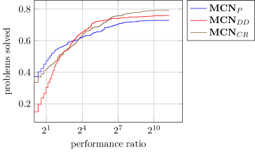
Figure 9: Performance Profile

In Table 3 and Table 4 the number of solved instance and the average runtimes, respectively, are given. The runtime differences of the different approaches depending on the setting of the instances are quite significant. E.g. for $|V|=40$ and budget setting 3-3-3 the MCN_P finishes an instance in about 12 seconds on average, while MCN_CR takes more than three-quarters of an hour. On the other hand, for $|V|=60$ and setting 3-1-3 this runtime observation is completely flipped around. On 72% of the instances with 20 to 40 nodes, the MCN_P was solved first. Interestingly, for the 3-1-3 and 3-3-1 setting MCN_CR seems to scale very well for increasing $|V|$, while both quantified programming approaches quickly fall behind. However, for the 1-3-3 setting both quantified programming approaches dominate MCN_CR, and in particular on the 2-2-2 instances the MCN_DD shows its potential. Generally speaking, the quantified programming approaches seem to be preferable on instances with small $\Omega$, i.e. a small number of vaccination options, while for large $\Omega$ the MCN_CR approach performs better. In Figure 9 we provide the performance profile [DM02]: for each solution approach the percentage of the $600$ instances is shown that are solved within a certain time relative to the fastest of the approaches. For example, on about 47% of the instances MCN_P spent at most twice as much time as the fastest approach.

Another benefit of the quantified programming approaches is the existence of an incumbent solution when the runtime is exceeded rather than only a bound obtained by MCN_CR: The incumbent solutions of MCN_DD (MCN_P) instances that hit the time limit but where solved to optimality with MCN_CR, where in 70% (65%) of the cases the optimal solution. And again we want to stress that our approach requires no domain knowledge, dualization or other preprocessing techniques, but only the ability to state the problem as QIP+.

For the multistage variants we only can compare our own methods, i.e. the two modeling formulations with and without the decision-dependent uncertainty set. For $|V|\in\{20,40,60\}$ and only using the budget settings with $\Phi\geq 2$ the same instances as used before are expanded to multistage instances as described in Section 5. Runtimes and the number of solved instances are shown in Table 5. For instances with $|V|\leq 40$ the MCN_P formulation is solved in all cases.

Table 5: Average runtime per instances (and number of solved instances) of the different multistage approaches

$|V|$		1-3-3		2-2-2		3-3-1		3-3-3
20	MCNP	3.5	(20)	2.0	(20)	16.0	(20)	14.4	(20)
	MCNDD	39.8	(20)	13.1	(20)	529.1	(20)	60.3	(20)
40	MCNP	193.6	(20)	18.8	(20)	2648.3	(20)	2645.4	(20)
	MCNDD	1489.1	(20)	273.6	(20)	7067.3	(1)	7200.0	(0)
60	MCNP	5916.0	(11)	1196.5	(20)	7200.0	(0)	7200.0	(0)
	MCNDD	7200.0	(0)	1634.1	(20)	7200.0	(0)	7200.0	(0)

In the case were all three budgets are set to $2$ all instances up to $|V|=60$ can be solved using either formulation. Similar to the observations obtained for the three stage case, the performance of the MCN_DD deteriorates with increasing $\Omega$. One reason is that an increased $\Omega$ results in a larger search space in the early decision stages, which is explored in a more clever fashion in the non-decision-dependent formulation, via the presented relaxation techniques, which is not applicable in the MCN_DD case.

7 Conclusion and Outlook

Quantified programs, which are linear programs with ordered variables that are either existentially or universally quantified, provide a convenient framework for multistage optimization under uncertainty. We presented QIP and the augmented version QIP+ that allows discrete uncertainty sets restricted by some polytope which manifestation even can be decision-dependent in an even more compact and straightforward manner. We presented a general, game-tree search based, solution approach and this way provide an easily accessible model-and-run approach for multistage robust discrete optimization with mixed-integer recourse variables in the final decision stage. In particular, there is no longer the need for tedious reformulation and dualization procedures that turn out to be in vain as soon as parts of the model change. Using the example of the multilevel critical node problem, we showcased that our solver provides a solid baseline while only having to state the problem in the most straightforward manner. Another major advantage of our search-based approach is the possibility to retrieve incumbent solutions, rather than bounds from a row-and-column generation approach. Furthermore, multistage extensions—that exceed the standard two-stage approach—are easily realizable in order to collect first insight into model structures while obtaining optimal solutions rather than approximations.

In particular for the novel QIP+ several challenges remain to be tackled by future research that will push the performance of the general search-based approach even further. To this end relaxation and branching techniques need to be developed that take the decision-dependent nature of the QIP+ into account. Furthermore, standard elimination techniques need to be reconsidered and the great potential of being able to learn universal constraints and propagate universal variables has to be exploited more effectively. Providing callbacks and allow the user to actively influence branching decisions can also be a successfully way to make use of our general framework while taking advantage of domain specific knowledge. Another important research direction is the availability of certificates that allow to better comprehend the solution or even its optimality.

8 Acknowledgments

This research was partially funded by the Deutsche Forschungsgemeinschaft (DFG, German Research Foundation) - 399489083.

Appendix A QLP File Format

For the QIP+ given by

$$\boldsymbol{c}^{\top}\boldsymbol{x}\,:\quad \min\ x_{1}+2x_{2}-5x_{3}+x_{4}$$

$$\boldsymbol{Q}\circ\mathcal{D}\,:\quad \exists\,x_{1}\in\{0,1,2\}\ \exists\,x_{2}\in\{0,1\}\ \forall\,x_{3}\in\{0,1\}\ \exists\,x_{4}\in[0,1]$$

$$A^{\exists}\boldsymbol{x}\leq\boldsymbol{b}^{\exists}\,:\quad \begin{pmatrix}1&-2&1&-1\\ -1&1&1&-1\end{pmatrix}\begin{pmatrix}x_{1}\\ x_{2}\\ x_{3}\\ x_{4}\end{pmatrix}\leq\begin{pmatrix}1\\ 1\end{pmatrix}\,$$

$$A^{\forall}\boldsymbol{x}\leq\boldsymbol{b}^{\forall}\,:\quad \begin{pmatrix}1&0&-1&0\end{pmatrix}\begin{pmatrix}x_{1}\\ x_{2}\\ x_{3}\\ x_{4}\end{pmatrix}\leq\begin{pmatrix}1\end{pmatrix}$$

the corresponding QLP file looks as follows:

MINIMIZE

x1 +2x2 -5x3 +x4

SUBJECT TO

x1 -2x2 +x3 -x4 <= 1

-x1 + x2 +x3 -x4 <= 1

UNCERTAINTY SUBJECT TO

x1 - x3 <= 1

BOUNDS

0 <= x1 <= 2

0 <= x2 <= 1

0 <= x3 <= 1

0 <= x4 <= 1

BINARIES

x2 x3

GENERAL

x1

EXISTS

x1 x2 x4

ALL

x3

ORDER

x1 x2 x3 x4

END

The corresponding solution file looks as follows:

⬇

<?xml version = ”1.0” encoding=”UTF-8” standalone=”yes”?>

<YasolSolution version=”1”>

<header

ProblemName=”Example.qlp”

SolutionName=”Example.qlp.sol”

ObjectiveValue=”-1.000000”

Runtime=”0.030seconds”

DecisionNodes=”8”

PropagationSteps=”11”

LearntConstraints=”5”/>

<quality

SolutionStatus=”OPTIMAL”

Gap=”0.000000”/>

<variables>

<variable name=”x1” index=”0-1” value=”2” block=”1”/>

<variable name=”x2” index=”2” value=”1” block=”1”/>

<variable name=”x3” index=”3” value=”1” block=”2”/>

<variable name=”x4” index=”4” value=”0.000000” block=”3”/>

</variables>

</YasolSolution>

References

- [Ach07] T. Achterberg. Conflict analysis in mixed integer programming. Discrete Optimization, 4(1):4–20, 2007.
- [Ach09a] T. Achterberg. Scip: solving constraint integer programs. Mathematical Programming Computation, 1(1):1–41, 2009.
- [Ach09b] Tobias Achterberg. Constraint Integer Programming. PhD thesis, TU Berlin, 2009.
- [AKM05] T. Achterberg, T. Koch, and A. Martin. Branching rules revisited. Operations Research Letters, 33(1):42–54, 2005.
- [AN77] S.G. Akl and M.M. Newborn. The principal continuation and the killer heuristic. In Proceedings of the 1977 annual conference, ACM ’77, Seattle, Washington, USA, pages 466–473, 1977.
- [BCLT21] A. Baggio, M. Carvalho, A. Lodi, and A. Tramontani. Multilevel approaches for the critical node problem. Operations Research, 69(2):486–508, 2021.
- [BD16] D. Bertsimas and I. Dunning. Multistage robust mixed-integer optimization with adaptive partitions. Operations Research, 64(4):980–998, 2016.
- [Ben62] J.F. Benders. Partitioning procedures for solving mixed-variables programming problems ‘. Numerische Mathematik, 4(1):238–252, 1962.
- [BG15] D. Bertsimas and A. Georghiou. Design of near optimal decision rules in multistage adaptive mixed-integer optimization. Operations Research, 63(3):610–627, 2015.
- [BIP10] D. Bertsimas, D.A. Iancu, and P.A. Parrilo. Optimality of affine policies in multistage robust optimization. Mathematics of Operations Research, 35(2):363–394, 2010.
- [BJLS21] O. Beyersdorff, M. Janota, F. Lonsing, and M. Seidl. Quantified boolean formulas. In Handbook of Satisfiability, pages 1177–1221. IOS Press, 2021.
- [BS04] D. Bertsimas and M. Sim. The price of robustness. Operations research, 52(1):35–53, 2004.
- [BTGGN04] A. Ben-Tal, A. Goryashko, E. Guslitzer, and A. Nemirovski. Adjustable robust solutions of uncertain linear programs. Mathematical Programming, 99(2):351–376, 2004.
- [BTGS09] A. Ben-Tal, B. Golany, and S. Shtern. Robust multi-echelon multi-period inventory control. European Journal of Operational Research, 199(3):922–935, 2009.
- [BTN02] A. Ben-Tal and A. Nemirovski. Robust optimization - methodology and applications. Mathematical Programming, 92(3):453–480, 2002.
- [CM83] M.S. Campbell and T.A. Marsland. A comparison of minimax tree search algorithms. Artificial Intelligence, 20(4):347 – 367, 1983.
- [CSGG02] M. Cadoli, M. Schaerf, A. Giovanardi, and M. Giovanardi. An algorithm to evaluate quantified boolean formulae and its experimental evaluation. Journal of Automated Reasoning, 28(2):101–142, 2002.
- [CSX20] Z. Chen, M. Sim, and P. Xiong. Robust stochastic optimization made easy with rsome. Management Science, 66(8):3329–3339, 2020.
- [CZ09] X. Chen and Y. Zhang. Uncertain linear programs: Extended affinely adjustable robust counterparts. Operations Research, 57(6):1469–1482, 2009.
- [DI15] E. Delage and D.A. Iancu. Robust multistage decision making. In The Operations Research Revolution, pages 20–46. INFORMS, 2015.
- [DM02] Elizabeth D Dolan and Jorge J Moré. Benchmarking optimization software with performance profiles. Mathematical programming, 91(2):201–213, 2002.
- [Dun16] I. Dunning. Advances in robust and adaptive optimization: algorithms, software, and insights. PhD thesis, Massachusetts Institute of Technology, 2016.
- [EHL+17] T. Ederer, M. Hartisch, U. Lorenz, T. Opfer, and J. Wolf. Yasol: An open source solver for quantified mixed integer programs. In Advances in Computer Games, pages 224–233. Springer, 2017.
- [FFZ21] W. Feng, Y. Feng, and Q. Zhang. Multistage robust mixed-integer optimization under endogenous uncertainty. European Journal of Operational Research, 294(2):460–475, 2021.
- [GH21] M. Goerigk and M. Hartisch. Multistage robust discrete optimization via quantified integer programming. Computers & Operations Research, 135(105434):1–13, 2021.
- [GKM+15] G. Gamrath, T. Koch, A. Martin, M. Miltenberger, and D. Weninger. Progress in presolving for mixed integer programming. Mathematical Programming Computation, 7(4):367–398, 2015.
- [GKW19] A. Georghiou, D. Kuhn, and W. Wiesemann. The decision rule approach to optimization under uncertainty: methodology and applications. Computational Management Science, 16(4):545–576, 2019.
- [GMT14] V. Gabrel, C. Murat, and A. Thiele. Recent advances in robust optimization: An overview. European Journal of Operational Research, 235(3):471–483, 2014.
- [GNRS08] I.P. Gent, P. Nightingale, A. Rowley, and K. Stergiou. Solving quantified constraint satisfaction problems. Artificial Intelligence, 172(6-7):738–771, 2008.
- [GNT03] E. Giunchiglia, M. Narizzano, and A. Tacchella. Backjumping for quantified boolean logic satisfiability. Artificial Intelligence, 145(1):99–120, 2003.
- [GPS95] R. Gerber, W. Pugh, and M. Saksena. Parametric dispatching of hard real-time tasks. IEEE transactions on computers, 44(3):471–479, 1995.
- [GS11] J. Goh and M. Sim. Robust optimization made easy with rome. Operations Research, 59(4):973–985, 2011.
- [GS16] M. Goerigk and A. Schöbel. Algorithm engineering in robust optimization. In Algorithm Engineering, pages 245–279. Springer International Publishing, Cham, 2016.
- [GYdH15] B.L. Gorissen, İ. Yanıkoğlu, and D. den Hertog. A practical guide to robust optimization. Omega, 53:124–137, 2015.
- [Har20] M. Hartisch. Quantified Integer Programming with Polyhedral and Decision-Dependent Uncertainty. PhD thesis, University of Siegen, Germany, 2020.
- [Har21] M. Hartisch. Adaptive relaxations for multistage robust optimization. In Pacific Rim International Conference on Artificial Intelligence, pages 485–499. Springer, 2021.
- [HELW16] M. Hartisch, T. Ederer, U. Lorenz, and J. Wolf. Quantified integer programs with polyhedral uncertainty set. In International Conference on Computers and Games, pages 156–166. Springer, 2016.
- [HJL+15] M. Heule, M. Järvisalo, F. Lonsing, M. Seidl, and A. Biere. Clause elimination for sat and qsat. Journal of Artificial Intelligence Research, 53:127–168, 2015.
- [HL19] M. Hartisch and U. Lorenz. Mastering uncertainty: towards robust multistage optimization with decision dependent uncertainty. In Pacific Rim International Conference on Artificial Intelligence, pages 446–458. Springer, 2019.
- [HL20] M. Hartisch and U. Lorenz. A novel application for game tree search - exploiting pruning mechanisms for quantified integer programs. In T. Cazenave, J. van den Herik, A. Saffidine, and I-C. Wu, editors, Advances in Computer Games, pages 66–78, Cham, 2020. Springer International Publishing.
- [HSB14] Marijn JH Heule, Martina Seidl, and Armin Biere. A unified proof system for qbf preprocessing. In International Joint Conference on Automated Reasoning, pages 91–106. Springer, 2014.
- [IJMS16] A. Ignatiev, M. Janota, and J. Marques-Silva. Quantified maximum satisfiability. Constraints, 21(2):277–302, 2016.
- [Jan18] M. Janota. Towards generalization in qbf solving via machine learning. In Proceedings of the AAAI Conference on Artificial Intelligence, 2018.
- [JKMSC16] M. Janota, W. Klieber, J. Marques-Silva, and E. Clarke. Solving qbf with counterexample guided refinement. Artif. Intell., 234:1 – 25, 2016.
- [JMS15a] M. Janota and J. Marques-Silva. Expansion-based qbf solving versus q-resolution. Theoretical Computer Science, 577:25–42, 2015.
- [JMS15b] M. Janota and J. Marques-Silva. Solving qbf by clause selection. In Proceedings of the 24th International Joint Conference on Artificial Intelligence, pages 325–331, 2015.
- [Kaw96] Y. Kawano. Using similar positions to search game trees. Games of No Chance, 29:193–202, 1996.
- [KM75] Donald E. Knuth and Ronald W. Moore. An analysis of alpha-beta pruning. Artificial Intelligence, 6(4):293–326, 1975.
- [KWG11] D. Kuhn, W. Wiesemann, and A. Georghiou. Primal and dual linear decision rules in stochastic and robust optimization. Mathematical Programming, 130(1):177–209, 2011.
- [LBB+15] F. Lonsing, F. Bacchus, A. Biere, U. Egly, and M. Seidl. Enhancing search-based qbf solving by dynamic blocked clause elimination. In Logic for Programming, Artificial Intelligence, and Reasoning, pages 418–433. Springer Heidelberg Berlin, 2015.
- [LE17] F. Lonsing and U. Egly. Depqbf 6.0: A search-based qbf solver beyond traditional qcdcl. In International Conference on Automated Deduction, pages 371–384. Springer International Publishing, Cham, 2017.
- [LE19] F. Lonsing and U. Egly. Qratpre+: Effective qbf preprocessing via strong redundancy properties. In International Conference on Theory and Applications of Satisfiability Testing, pages 203–210. Springer International Publishing, Cham, 2019.
- [LEvG13] F. Lonsing, U. Egly, and A. van Gelder. Efficient clause learning for quantified boolean formulas via qbf pseudo unit propagation. In International Conference on Theory and Applications of Satisfiability Testing, pages 100–115. Springer, 2013.
- [LG18] N.H. Lappas and C.E. Gounaris. Robust optimization for decision-making under endogenous uncertainty. Computers & Chemical Engineering, 111:252–266, 2018.
- [LLM+21] M. Leitner, I. Ljubić, M. Monaci, M. Sinnl, and K. Tanınmış. An exact method for fortification games. arXiv preprint arXiv:2111.13400, 2021.
- [LLMS09] C. Liebchen, M. Lübbecke, R. Möhring, and S. Stiller. The concept of recoverable robustness, linear programming recovery, and railway applications. In Robust and online large-scale optimization, pages 1–27. Springer Berlin Heidelberg, 2009.
- [LRSL19] G. Lederman, M. Rabe, S. Seshia, and E.A. Lee. Learning heuristics for quantified boolean formulas through reinforcement learning. In International Conference on Learning Representations, 2019.
- [LSvG16] F. Lonsing, M. Seidl, and A. van Gelder. The qbf gallery: Behind the scenes. Artificial Intelligence, 237:92–114, 2016.
- [LW15] U. Lorenz and J. Wolf. Solving multistage quantified linear optimization problems with the alpha–beta nested benders decomposition. EURO Journal on Computational Optimization, 3(4):349–370, 2015.
- [MMZ+01] M.W. Moskewicz, C.F. Madigan, Y. Zhao, L. Zhang, and S. Malik. Chaff: Engineering an efficient sat solver. In Proceedings of the 38th annual Design Automation Conference, pages 530–535, 2001.
- [NS18] O. Nohadani and K. Sharma. Optimization under decision-dependent uncertainty. SIAM Journal on Optimization, 28(2):1773–1795, 2018.
- [P.14] Michael P. Robust combinatorial optimization with variable cost uncertainty. European Journal of Operational Research, 237(3):836–845, 2014.
- [Pap85] C.H. Papadimitriou. Games against nature. Journal of Computer and System Sciences, 31(2):288–301, 1985.
- [PdB01] W. Pijls and A. de Bruin. Game tree algorithms and solution trees. Theoretical Computer Science, 252(1):197–215, 2001.
- [PdH16] K. Postek and D. den Hertog. Multistage adjustable robust mixed-integer optimization via iterative splitting of the uncertainty set. INFORMS Journal on Computing, 28(3):553–574, 2016.
- [Pea80] J. Pearl. Scout: A simple game-searching algorithm with proven optimal properties. In AAAI, pages 143–145, 1980.
- [Pos14] M. Poss. Robust combinatorial optimization with variable cost uncertainty. European Journal of Operational Research, 237(3):836–845, 2014.
- [PS19] L. Pulina and M. Seidl. The 2016 and 2017 qbf solvers evaluations (qbfeval’16 and qbfeval’17). Artificial Intelligence, 274:224–248, 2019.
- [PSPDB96a] A. Plaat, J. Schaeffer, W. Pijls, and A. De Bruin. Best-first fixed-depth minimax algorithms. Artificial Intelligence, 87(1-2):255–293, 1996.
- [PSPdB96b] A. Plaat, J. Schaeffer, W. Pijls, and A. de Bruin. Best-first fixed-depth minimax algorithms. Artificial Intelligence, 87(1):255 – 293, 1996.
- [PSS19a] T. Peitl, F. Slivovsky, and S. Szeider. Dependency learning for qbf. Journal of Artificial Intelligence Research, 65:180–208, 2019.
- [PSS19b] T. Peitl, F. Slivovsky, and S. Szeider. Long-distance q-resolution with dependency schemes. Journal of Automated Reasoning, 63(1):127–155, 2019.
- [Rei83a] A. Reinefeld. An improvement to the scout tree search algorithm. ICGA Journal, 6(4):4–14, 1983.
- [Rei83b] A. Reinefeld. An improvement to the scout tree search algorithm. ICGA Journal, 6(4):4–14, 1983.
- [RT15] M.N. Rabe and L. Tentrup. Caqe: a certifying qbf solver. In 2015 Formal Methods in Computer-Aided Design (FMCAD), pages 136–143. IEEE, 2015.
- [Sch89] J. Schaeffer. The history heuristic and alpha-beta search enhancements in practice. IEEE Trans. Pattern Anal. Mach. Intell., 11(11):1203–1212, 1989.
- [Sha11] A. Shapiro. A dynamic programming approach to adjustable robust optimization. Operations Research Letters, 39(2):83–87, 2011.
- [Sto79] G.C. Stockman. A minimax algorithm better than alpha-beta? Artificial Intelligence, 12(2):179 – 196, 1979.
- [Sub03] K. Subramani. An analysis of quantified linear programs. In International Conference on Discrete Mathematics and Theoretical Computer Science, pages 265–277. Springer, 2003.
- [Sub04] K. Subramani. Analyzing selected quantified integer programs. In International Joint Conference on Automated Reasoning, pages 342–356. Springer, 2004.
- [Ten19] L. Tentrup. Caqe and quabs: Abstraction based qbf solvers. Journal on Satisfiability, Boolean Modeling and Computation, 11(1):155–210, 2019.
- [TTE09] A. Thiele, T. Terry, and M. Epelman. Robust linear optimization with recourse. Rapport Technique, pages 4–37, 2009.
- [VJE20] P. Vayanos, Q. Jin, and G. Elissaios. Roc++: Robust optimization in c++. arXiv preprint arXiv:2006.08741, 2020.
- [WBH21] J. Witzig, T. Berthold, and S. Heinz. Computational aspects of infeasibility analysis in mixed integer programming. Mathematical Programming Computation, 13(4):753–785, 2021.
- [Wet74] R.J.-B. Wets. Stochastic programs with fixed recourse: The equivalent deterministic program. SIAM review, 16(3):309–339, 1974.
- [WM21] J. Wiebe and R. Misener. Romodel: Modeling robust optimization problems in pyomo. Optimization and Engineering, pages 1–22, 2021.
- [WRMB17] R. Wimmer, S. Reimer, P. Marin, and B. Becker. Hqspre–an effective preprocessor for qbf and dqbf. In International Conference on Tools and Algorithms for the Construction and Analysis of Systems, pages 373–390. Springer Berlin Heidelberg, 2017.
- [WvdWvdHU04] M.H.M. Winands, E.C.D. van der Werf, H.J. van den Herik, and J.W.H.M. Uiterwijk. The relative history heuristic. In Computers and Games, 4th International Conference, CG 2004, pages 262–272, 2004.
- [YGdH19] İ. Yanıkoğlu, B.L. Gorissen, and D. den Hertog. A survey of adjustable robust optimization. European Journal of Operational Research, 277(3):799–813, 2019.
- [ZDHS18] J. Zhen, D. Den Hertog, and M. Sim. Adjustable robust optimization via fourier–motzkin elimination. Operations Research, 66(4):1086–1100, 2018.
- [ZF20] Q. Zhang and W. Feng. A unified framework for adjustable robust optimization with endogenous uncertainty. AIChE Journal, 66(12):e17047, 2020.
- [ZKG+17] Xiaojing Zhang, Maryam Kamgarpour, Angelos Georghiou, P. Goulart, and J. Lygeros. Robust optimal control with adjustable uncertainty sets. Automatica, 75:249–259, 2017.
- [ZM02] L. Zhang and S. Malik. Conflict driven learning in a quantified boolean satisfiability solver. In Proceedings of the 2002 IEEE/ACM international conference on Computer-aided design, pages 442–449, 2002.