Lower-than-expected flare temperatures for TRAPPIST-1

Abstract

Aims. Stellar flares emit thermal and nonthermal radiation in the X-ray and ultraviolet (UV) regime. Although high energetic radiation from flares is a potential threat to exoplanet atmospheres and may lead to surface sterilization, it might also provide the extra energy for low-mass stars needed to trigger and sustain prebiotic chemistry. Despite the UV continuum emission being constrained partly by the flare temperature, few efforts have been made to determine the flare temperature for ultra-cool M-dwarfs. We investigate two flares on TRAPPIST-1, an ultra-cool dwarf star that hosts seven exoplanets of which three lie within its habitable zone. The flares are detected in all four passbands of the MuSCAT2 instrument allowing a determination of their temperatures and bolometric energies.

Methods. We analyzed the light curves of the MuSCAT1 (multicolor simultaneous camera for studying atmospheres of transiting exoplanets) and MuSCAT2 instruments obtained between 2016 and 2021 in $g,r,i,z_{\mathrm{s}}$-filters. We conducted an automated flare search and visually confirmed possible flare events. The black body temperatures were inferred directly from the spectral energy distribution (SED) by extrapolating the filter-specific flux. We studied the temperature evolution, the global temperature, and the peak temperature of both flares.

Results. White-light M-dwarf flares are frequently described in the literature by a black body with a temperature of 9000-10000 K. For the first time we infer effective black body temperatures of flares that occurred on TRAPPIST-1. The black body temperatures for the two TRAPPIST-1 flares derived from the SED are consistent with $T_{\mathrm{SED}}=7940_{-390}^{+430}$ K and $T_{\mathrm{SED}}=6030_{-270}^{+300}$ K. The flare black body temperatures at the peak are also calculated from the peak SED yielding $T_{\mathrm{SEDp}}=13620_{-1220}^{1520}$ K and $T_{\mathrm{SEDp}}=8290_{-550}^{+660}$ K. We update the flare frequency distribution of TRAPPIST-1 and discuss the impacts of lower black body temperatures on exoplanet habitability.

Conclusions. We show that for the ultra-cool M-dwarf TRAPPIST-1 the flare black body temperatures associated with the total continuum emission are lower and not consistent with the usually adopted assumption of 9000-10000 K in the context of exoplanet research. For the peak emission, both flares seem to be consistent with the typical range from 9000 to 14000 K, respectively. This could imply different and faster cooling mechanisms. Further multi-color observations are needed to investigate whether or not our observations are a general characteristic of ultra-cool M-dwarfs. This would have significant implications for the habitability of exoplanets around these stars because the UV surface flux is likely to be overestimated by the models with higher flare temperatures.

1 Introduction

M-dwarfs are prime targets for the search for habitable conditions, that is, rocky planets in the habitable zone of the stars. The small stellar radius and low effective temperatures of M-dwarfs permit not only the detection of habitable planets but also the atmospheric characterization of those in close-in orbits (e.g. Kaltenegger & Traub, 2009, and references therein). M-dwarfs represent roughly $\leavevmode\nobreak\ 73\%$ of all stars (Dole, 1964; Henry et al., 2006, 2018). Late M-dwarfs, including ultra-cool M-dwarfs, have masses $M_{*}\leq 0.2M_{\odot}$ and effective temperatures $T_{\mathrm{eff}}\leq 3000$ K (Gillon et al., 2017). Ultra-cool dwarfs are stellar and substellar objects with spectral type later than M7V (Kirkpatrick et al., 1995, 1997). Mid and early M-dwarfs are more massive, $0.2M_{\odot}<M_{*}\leq 0.4M_{\odot}$, $0.4M_{\odot}<M_{*}\leq 0.6M_{\odot}$ respectively, and thus have surface temperatures of up to 3900 K (Heath et al., 1999; Farihi et al., 2006). Ground-based targeted searches such as MEarth (Irwin et al., 2009), TRAPPIST (Gillon et al., 2013), ExTrA (Bonfils et al., 2015) and SPECULOOS (Sebastian et al., 2020), as well as the space missions Kepler (Koch et al., 2010), K2 (Howell et al., 2014), and TESS (Ricker et al., 2014), have boosted the discoveries of exoplanets around nearby M-dwarfs. Consequently, there is growing interest in putting constraints on the flare rates of the host stars and the respective flare energies, temperatures, and areas (e.g Fuhrmeister et al., 2008; Schmidt et al., 2016; Davenport, 2016; Vida et al., 2017; Günther et al., 2020; Howard et al., 2020; Johnson et al., 2021) in order to understand how these can affect planetary atmospheres and the prospects of searching for habitable conditions.

Stellar flares are explosive magnetic reconnection events (Pettersen, 1989) occurring in main sequence (MS) stars with convective envelopes. When opposing magnetic field lines approach each other, they are prone to reconnect and release the energy that was stored in the magnetic field in the form of accelerated particles and electromagnetic radiation. These stochastic events have a duration ranging from minutes to several hours (Benz, 2017)[e.g.][and references therein]. The flare occurrence frequency and the released energy are both dependent on the magnetic field of the stellar surface, which is known to decrease with stellar age for MS stars (Reiners et al., 2022). Due to the loss of angular momentum, the stellar dynamo quiets during the star’s lifetime (Skumanich, 1972). For low-mass stars, this process takes longer than for solar type stars and thus, in comparison, low-mass stars experience a prolonged active time (West et al., 2008), they produce high UV and X-ray flux over longer periods (Audard et al., 2000; Hawley et al., 2014), which can alter the atmospheres of close-by planets and might be a serious threat to surface life (Segura et al., 2010; Tilley et al., 2019). Other studies suggest that additional UV flux from stellar flares might trigger and drive prebiotic chemistry on planetary surfaces (Ranjan et al., 2017; Rimmer et al., 2018). Several recent studies of stellar flares on nearby M-dwarfs with planetary companions address surface habitability (Ribas et al., 2016; O’Malley-James & Kaltenegger, 2017; Meadows et al., 2018; Vida et al., 2019; Glazier et al., 2020) and use constant flare temperatures of $T_{\mathrm{eff}}=9000-10000$ K. However, a lower or higher flare temperature would impact the UV flux models for the star and therefore the flux incident on the planetary companions.

The primary output of flares are accelerated particles, which then precipitate back on the chromosphere of the star, emitting nonthermal radiation and subsequently heat the chromospheric plasma (Benz & Güdel, 2010; Aschwanden et al., 2017; Benz, 2017). The amount of heating differs locally and is strongest at the footpoints of the magnetic loop after reconnection. This local heating gives rise to thermal continuum emission and line emission in the optical, UV, and soft X-ray regime (Benz & Güdel, 2010; Kowalski et al., 2013; Aschwanden et al., 2017). One example is the H$\alpha$ line. At the footpoints of the magnetic fields, accelerated electrons and protons will recombine producing hydrogen emission lines, the so-called H$\alpha$ ribbons (Kowalski et al., 2013). The main contribution to the total energy budget of a flare comes from the white-light continuum emission (Benz & Güdel, 2010; Aschwanden et al., 2017). The total energy budget is frequently estimated by a black body of effective temperature $T_{\mathrm{eff}}=9000-10000$ K (Hawley & Pettersen, 1991; Kretzschmar, 2011; Kowalski et al., 2013; Shibayama et al., 2013; Davenport, 2016; Paudel et al., 2018; Howard et al., 2018; Jackman et al., 2018, 2019; Günther et al., 2020) . While this knowledge relies mainly on magnetically active M-dwarfs (dMe stars) with spectral types dM3e-dM4.5e from spectroscopic and photometric observations(e.g. Kowalski et al., 2013, and references therein), it is usually assumed that flares on ultra-cool M-dwarfs like TRAPPIST-1 with spectral type M7.5V behave similarly (Paudel et al., 2018; Günther et al., 2020; Glazier et al., 2020).

Multi-passband photometry is a useful tool for determining continuum black body temperatures of stellar flares (Hawley et al., 2003; Kowalski et al., 2013; Howard et al., 2020). The black body temperature of stellar flares is not constant and should be understood as an energy budget of the continuum emission. As flares are subject to different physical processes in different atmospheric layers, it is nontrivial to attribute a single temperature characterizing the flare. If flares are observed in several photometric filters, recent methods can be employed to retrieve black body temperatures (Howard et al., 2020). For typical active M-dwarf stars spectroscopic and photometric observations are consistent with a black body with temperatures of 9000-14000 K at the peak and 5500-7000 K in the gradual phase (Kowalski et al., 2013). Howard et al. (2020) investigated a large sample of stars with photometric flares and spectral types of M0-M7V. These authors found the total temperature averaged over their sample to be $T_{\mathrm{eff}}=11000\begin{subarray}{c}+3500\\ -2600\end{subarray}$ K and at peak $T_{\mathrm{eff}}=14000\begin{subarray}{c}+8300\\ -3400\end{subarray}$ K.

For studying flares on low-mass stars in the context of exoplanet research, the most promising target is TRAPPIST-1. This target is a well-studied late M-dwarf with spectral type M7.5V (Gizis et al., 2000) and is known to host seven rocky exoplanets of which three lie within the habitable zone, which is the zone where the surface flux is just right for water to be liquid (Gillon et al., 2016, 2017; Luger et al., 2017). Because TRAPPIST-1 flares frequently, with a flare with an energy above $10^{29}$ erg occurring every 1-2 days (Paudel et al., 2018), the impact of its flaring activity on the atmospheres of its orbiting exoplanets is being investigated (Vida et al., 2017; O’Malley-James & Kaltenegger, 2017; Paudel et al., 2018; Glazier et al., 2020; Estrela et al., 2020). Paudel et al. (2018) analysed K2 data for TRAPPIST-1 and detected 39 flares, and a superflare rate of $4.4\begin{subarray}{c}+2.0//-0.2\end{subarray}$ flares per year. A flare is considered a superflare if it reaches bolometric energies of $10^{33}-10^{38}$ erg (Shibayama et al., 2013). Glazier et al. (2020) did not detect flares in a two-year survey with Everyscope, an array of small telescopes imaging the entire accessible sky all at once (Law et al., 2016; Ratzloff et al., 2019). Glazier et al. (2020) and Paudel et al. (2018) argue that the possible atmospheres of the planets in the habitable zone of TRAPPIST-1 are, with the current flare rate, not in danger of complete ozone depletion, but also suggest that the UV flux from TRAPPIST-1 is not enough to trigger and sustain abiogenesis. Tilley et al. (2019) showed that UV radiation and proton fluxes from frequent flaring can deplete the ozone layer of an Earth-like planet almost entirely over timescales of several million years. Estrela et al. (2020) examined the impact of the UV radiation from flares on the potentially habitable planets of TRAPPIST-1. These authors argue that UV-sensitive organisms could survive if the planet has an ozone layer or if their natural living environment is at least 8m below surface ocean level. These studies highlight the importance of considering flares when assessing the habitability of a planet. Despite the growing interest in flaring processes of ultra-cool M-dwarfs and their subsequent UV radiation, the flare temperature of the continuum emission remain uncertain for late M-dwarfs. For a L-dwarf (L1V) flare, Gizis et al. (2013)found a black body spectrum consistent with an effective temperature of $T_{\mathrm{eff}}=8000\pm 2000$ K.

Here, we present an automated search for stellar flares on TRAPPIST-1 using MuSCAT1 (Multicolor simultaneous camera for studying atmospheres of transiting exoplanets) (Narita et al., 2015) and MuSCAT2 (Narita et al., 2019) data and the open source package AltaiPony (Ilin, 2021). For the first time using the simultaneous multi-color photometry of the MuSCAT instruments, we estimated effective black body temperatures of TRAPPIST-1 flares.

The paper is structured as follows: In Section 2, we present the instruments, observations and preparation of the photometric data. Section 3.1 describes the flare detection, and in Section 3, we describe the methods used to derive black body temperatures. The results are presented in Section 4 and discussed in Section 5. Finally, we summarize our findings in Section 6.

2 Observations

MuSCAT1 (M1) and MuSCAT2 (M2) (Multicolor Simultaneous Camera for studying Atmospheres of Transiting exoplanets) are part of the Global Multi-Color Photometric Monitoring Network for Exoplanetary Transits. M1 is mounted on the 1.88m telescope at the Okayama Astro-Complex in Japan and M2 is located at the Teide Observatory in Tenerife, Spain and mounted on the 1.52 m Telescopio Carlos Sánchez (TCS). While M1 permits the use of three photometric filters $g$, $r$, and $z_{\text{s}}$ at the same time, M2 observes in four band-passes simultaneously, namely $g$ (400-550 nm), $r$ (550-700 nm), $i$ (700-820 nm), and $z_{\text{s}}$ (820-920 nm) (Narita et al., 2015, 2019). M1 and M2 are equipped with 1024$\times$1024 pixel CCDs with a pixel scale of 0.36 and 0.44 arcsec/pixel, resulting in a field of view of 6.1$\times$6.1 arcmin and 7.4$\times$7.4 arcmin, respectively. Both instruments are used for follow-up observations of transiting exoplanets by for example TESS for confirmation and/or validation, and studies of exoplanet atmospheres. The data are reduced and optimized with the M2 transit pipeline (Parviainen et al., 2020). The pipeline covers the reduction of generic (nontransit) photometry, transit analysis, and more specific TESS follow-up analysis. Moreover, the pipeline tags exposures where any of the pixels inside a photometry aperture for a star are close to the linearity limit of the CCD. The exposures where either the target star or any of the comparison stars may be saturated are excluded from the analysis. The uncertainty on the data points is inferred using a rolling median with sigma clipping equivalent to the flux error determined by the PDCSAP pipeline for Kepler and TESS data. We estimate the average white noise scatter during the fitting in the pipeline, assuming the uncertainties do not change significantly during the night.

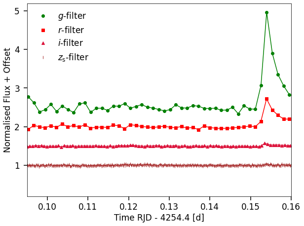
Figure 1: Light curve in all four filters of MuSCAT2 (M2) of Flare 1: The flare is visible in the $g$, $r$, and $i$ filter, whereas the S/N in the $z_{\mathrm{s}}$-filter is too low. To better distinguish between the four M2 channels, we add constant values to the flux. The time is given in days in reduced Julian date (RJD), RJD = BJD - 2454833 d where BJD is the barycentric Julian date.

For the analysis, we used 48 nights of M2 between 2018 and 2020, and 11 nights of M1 between 2016 and 2020, with an observation of 1-3 hours per night for both instruments. Thus, we had a total observation time of four days per filter for the M2 instrument; we refer to Table 3 for details.

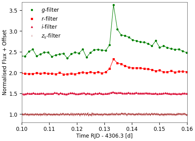
Figure 2: Light curve in all four filters of MuSCAT2 (M2) of Flare 2: The flare is visible in the $g$- and $r$-filter, whereas the S/N in the $i$- and $z_{\mathrm{s}}$-filter are too low. Time and flux are as indicated in Figure 1

We also consider the K2 data set of TRAPPIST-1 (Howell et al., 2014). Paudel et al. (2018) analyzed the short-cadence data of the K2 Campaign 12 (Gilliland et al., 2010) and report 39 flares. An overview of the data of TRAPPIST-1 for M1, M2 and K2 is given in the Appendix in Table 3. In Figure 1 and Figure 2 both flare light curves of M2 are shown in all four photometric bands.

3 Methods

3.1 Flare detection

For the flare detection we relied on the AltaiPony package (Ilin, 2021). The selection criteria were adopted from Chang et al. (2015), where every outlier with three subsequent data points exceeding the local $\sigma$-level by a factor of three, was considered a flare candidate. $\sigma$ represents the local standard deviation. To discriminate the real flares among the candidates found by the algorithm, the standard method is a flare injection recovery (hereafter FLIR), which constrains the probability of a given candidate being recovered in a given light curve. However, as the M2 data for TRAPPIST-1 suffer from strong variation in the photometric scatter due to weather, moon and telescope issues, we would have to perform the FLIR on every single observation night independently. For this reason, we first detected the flares with AltaiPony and afterwards, instead of performing FLIR on all light curves, we visually selected the flare candidates and adopted FLIR for M2 example light curves for each pass-band. The results of the FLIR of the M2 example light curves were used to explore the lower detection limit in bolometric energy. For M2 we obtained a detection limit of $E_{\mathrm{bol}}=0.74\times 10^{30}$ erg, see Appendix A.

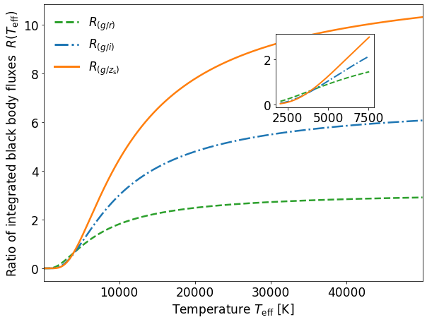
Figure 3: Ratio R of integrated fluxes observed in the MuSCAT band-passes uniquely determines the effective black body temperature of a flare. A black body of temperature $T_{\mathrm{eff}}$ is separately multiplied by the spectral response functions of the MuSCAT filters to produce the ratios $R_{j}$. We obtain different sensitivities for each filter pair: $R_{(g,r_{\mathrm{s}})}$ is theoretically more sensitive in temperatures below $5000$ K while $R_{(g,z_{\mathrm{s}})}$ may be sensitive to temperatures up to $50000$ K.

3.2 Flare temperatures

The color temperature of a stellar flare is defined as the effective continuum temperature associated with a black body inferred from its spectral properties (e.g. Howard et al., 2020, and references therein). To estimate the color temperatures for MuSCAT flares we applied two different methods. First, the MuSCAT instruments provide the opportunity with their different photometric filters to measure the spectral energy distribution (SED) of flare events, that is the energy emitted by the flare per unit area, time and wavelength. We attempted to extrapolate the SED leaving the effective temperature and the flaring area as free parameters. The flaring area parameter $a$ is given as a fraction of stellar radius and is the part of the stellar surface where the continuum emission of the flare is emitted. We assume it to be circular. The applied black body model can be found in the Appendix equation (20). To avoid confusion, we refer to the effective temperatures estimated from the SED as SED temperatures $T_{\mathrm{SED}}$. Second, we followed the methodology from Howard et al. (2020) c.f. Section 5, to infer the flare color temperature using only two different filters. The global flare temperature $T_{\mathrm{glob}}$ is defined as the black body effective temperature linked to the total amount of flux of the flare, whereas the peak temperature $T_{\mathrm{peak}}$ is the temperature associated with the average temperature inside the FWHM of the flare (Howard et al., 2020). The temperatures can be estimated for each multi-color data point yielding a time evolution in flare temperatures.

As we did not have any simultaneous flare observed with K2 at different bands, this analysis was done only for the MuSCAT instruments.

SED temperature method:

• We computed the flux of TRAPPIST-1 in each MuSCAT filter using the corresponding segments of the mega-MUSCLES semi-empirical model (Wilson et al., 2021) and calibrated the data to absolute fluxes using the Gaia DR2 catalog (Evans et al., 2018). For the calibration we followed Ilin et al. (2021), (c.f. Section 2.4.3). First, we integrated the mega-MUSCLES spectra over the Gaia G-band response function, and normalized the SED to the Gaia G-band flux for TRAPPIST-1. Integrating over the MuSCAT-band response curves, we obtained the fluxes in the MuSCAT2-bands.

• We then fit the relative flare light curve with the flare template aflare1 (Davenport et al., 2014). From the best-fit flare profile (cf. Section 3.3), we calculated the percentage flux change of TRAPPIST-1 during the flare.

• The flare SED was then obtained by multiplying the percentage flux change of the flare with the quiescent flux for any MuSCAT filter.

• We fit the flare SED with a black body model leaving the effective temperature and the flaring area as free parameters, c.f. Appendix Section C.1.

This task can be performed for both the total flare flux, that is, the flux arising from the combined rise, peak and decay phase, and the peak flare flux, which is the flux emitted at the peak of the flare.

Two-filter temperature method from Howard et al. (2020):

• We computed the radiation spectrum of a black body with temperature $T_{\mathrm{eff}}$ as a function of wavelength $\lambda$. We multiplied all filters separately with the black body spectrum and integrated them over the M1/M2 wavelength range to obtain the passband-specific flux. To account for the filter sensitivity we normalized the fluxes by dividing each calculated passband-specific flux by the total filter throughput.

• We took the ratios $R_{j}$ between the flux observed in all different filters, namely M2 $g$, $r$, $i$ and $z_{\mathrm{s}}$ where
  $j\in[(g/r),(g/i),(g/z_{\mathrm{s}})]$. By convention, we took every single ratio such that the flux of the filter with a higher central wavelength was in the denominator and the flux of the filter with a lower central wavelength is in the numerator. In total we had three ratio functions to probe the color temperatures $[R_{(g/r)},R_{(g/i)},R_{(g/z_{\mathrm{s}})}]$.

• This process was repeated for effective black body temperatures $T_{\mathrm{eff}}=[50,50000]$ K with $5$ K steps.

• To compute the effective black body temperatures of the observed flares, we inverted the different ratio functions such that we had the temperature as a function of the respective filter ratio $T_{\mathrm{eff}}(R_{j})$.

In Figure, 3 the ratio functions $R_{j}$ are plotted for all different filter combinations for the MuSCAT filters as a function of effective black body temperature $T_{\mathrm{eff}}$. The $R_{j}({T_{\mathrm{eff}}})$ functions indicate that the retrievable color temperature information is limited. Where $R_{j}({T_{\mathrm{eff}}})$ is getting asymptotic, we reach the $R_{j}$ specific sensitivity limit; see Table 7. Beyond these limits, we cannot give reasonable estimates of the color temperature. In comparison, the ratio functions approach the asymptote faster if the total covered wavelength range between the two filters is smaller.

Following, Hawley et al. (2003); Howard et al. (2020); Castellanos Durán & Kleint (2020) we calculated the wavelength-specific flux $F_{\lambda}$,

$$F_{\lambda}=\frac{A_{\mathrm{flare}}B_{\lambda}(T_{\mathrm{flare}})}{d^{2}}$$ (1)

where $A_{\mathrm{flare}}$ is the area of the flare, $B_{\lambda}(T_{\mathrm{flare}})$ is the black body spectrum of the flare with color temperature $T_{\mathrm{flare}}$, and $d$ is the distance of the star. $A_{\mathrm{flare}}$ does not depend on $\lambda$ (Günther et al., 2020; Howard et al., 2020), taking the ratios between two passband fluxes yields:

$$\centering\frac{F_{\lambda_{1}}}{F_{\lambda_{2}}}\approx\frac{B_{\lambda_{1}}(T_{\mathrm{flare}})}{B_{\lambda_{2}}(T_{\mathrm{flare}})}=R_{j}\@add@centering$$ (2)

With equation (2) we used the ratio functions to infer the temperatures for the observed flares. Following Howard et al. (2020), this could be done in three different ways. We first investigated the flare temperature epoch by epoch, and then the global flare temperature. Finally, and importantly, we examined the flare peak temperature. We employ the calculation of all three measures and probe their consistency with the SED temperatures from the total flux and the peak flux.

3.3 Equivalent duration

The equivalent duration ($ED$) is defined as the amount of time it would take the star in its quiescent state to produce the same amount of energy that is released in a flare event (Gershberg, 1972; Hunt-Walker et al., 2012). Thus, it is the time integral of the dimensionless flux,

$$ED=\int{\frac{F_{\text{flare}}-F_{\mathrm{q}}}{F_{\text{q}}}dt},$$ (3)

where $F_{\mathrm{q}}$ is the quiescent flux of the star and $F_{\mathrm{flare}}$ is the flux observed during the flare. To estimate the equivalent duration, we fit the flare template aflare1 (Davenport et al., 2014) to each selected flare and thus acquire a best-fit approximation using an MCMC approach (Foreman-Mackey et al., 2013). The analytic expressions for the flare template are given in Section B.1 in the Appendix. We used 5000 steps in the MCMC chain with 40 walkers, and discard the first 1000 steps as the burn-in phase. To put constraints on the parameters for the flare template (amplitude, peak time and full width at half maximum (FWHM)) we define Gaussian prior probability distributions, see appendix B.2. After the fitting process, we integrate the flare template with the best-fit parameters for each flare event over time and thus obtain the ED, making use of the trapezoidal sum for integration. In Figure 4 a flare profile fit is shown for the $r$-band.

Stellar flares are often multi-peaked (Günther et al., 2020) or show quasi-periodic pulsations (QPP) (Mathioudakis et al., 2003; Mitra-Kraev et al., 2005). We focused in this work on modeling classical single-peaked flare events and disregard periodic oscillations in the decay phase in our analysis because both would not affect our temperature estimation; c.f. Section 5.5.

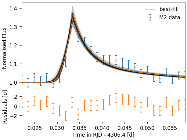
Figure 4: Flux profile fit of Flare 2 with M2 $r$-filter data: The orange curve indicates the best-fit using the flare template aflare1. The black lines show 100 random samples from the Markov chain. The lower panel shows the residuals between the observation and the model. The corresponding posterior probability distribution of the MCMC-fit is shown in Figure 13 of the Appendix. The lower panel reveals systematic errors in the residuals which might be due to superimposed flares or oscillations. This is further discussed in Section 5.

4 Results

We found no flares in the M1 data and two flares were observed in all four filters in the M2 data. Flare 1 had a bolometric energy of $E_{\mathrm{bol}}=2.99\times 10^{31}$ erg and occurred on August $25$ 2020 and Flare 2 had a bolometric energy of $E_{\mathrm{bol}}=1.51\times 10^{31}$ erg and occurred on October $15$ 2020. Both flares are shown in all passbands in Figure 1 and Figure 2, respectively.

4.1 SED temperatures

To infer the SED for our M2 flares, we used the methods described in Section 3.2.

The inferred SEDs for both flares are shown in Figure 5. The uncertainties were propagated from the best-fit of the flare flux profiles and the uncertainties of the mega-MUSCLES spectrum, as well as the uncertainties on the Gaia flux. To find a black body temperature consistent with the empirically measured filter fluxes, we used our black body model (c.f. equation (20) of the Appendix) and employed a fit to the data using emcee (Foreman-Mackey et al., 2013). We used 40 walkers and 25000 steps in the chain and discarded the first 5000 steps as the burn-in phase. The convergence was checked visually by plotting the chains against step number and by computing the integrated autocorrelation time (Sokal, 1996; Goodman & Weare, 2010; Foreman-Mackey et al., 2013). We report autocorrelation times of roughly 35 steps for each trial. The used prior probability distributions can be found in 5. In Figure 6 the combined posterior probability distributions for both flare samples are shown and reveal a satisfactory resolution of the expected degeneracy between the area parameter and the flare temperature. The posterior distributions overlap marginally for the flare area parameter but indicate that the flare temperatures are indeed different between the two flares. The best-fit temperatures are $T_{\mathrm{SED}}=7940\begin{subarray}{c}+430\\ -390\end{subarray}$ K for Flare 1 and $T_{\mathrm{SED}}=6030\begin{subarray}{c}+300\\ -270\end{subarray}$ K for Flare 2. The same task is performed for the peak temperatures yielding $T_{\mathrm{SEDp}}=13650\begin{subarray}{c}+1550\\ -1250\end{subarray}$ K for Flare 1 and $T_{\mathrm{SEDp}}=8300\begin{subarray}{c}+700\\ -550\end{subarray}$ for Flare 2. The best-fit area parameters to the SEDs are $a=0.266\begin{subarray}{c}+0.023\\ -0.021\end{subarray}$ for Flare 1 and $a=0.171\begin{subarray}{c}+0.019\\ -0.017\end{subarray}$ for Flare 2. And for the peak SED $a_{\mathrm{p}}=0.536\begin{subarray}{c}+0.062\\ -0.070\end{subarray}$ for Flare 1 and $a_{\mathrm{p}}=0.213\begin{subarray}{c}+0.027\\ 0.031\end{subarray}$ for Flare 2. The coverage of the stellar surface is represented in Table 1 and indicates that the flares cover up to $28\%$ of the surface of TRAPPIST-1 at the peak and in the combined rise, peak and gradual phases up to $8\%$.

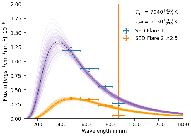
Figure 5: SED for the two observed flares in M2. The SEDs are fit with a model where the temperature $T_{\mathrm{eff}}$ and the area parameter $a$ are left as free parameters using emcee again. The flux in $z_{\mathrm{s}}$-filter is slightly inconsistent with the best-fit black bodies for both flares. The uncertainties of the model are indicated with shaded areas. The uncertainty bars in wavelength should be understood as the respective filter widths. The SED for Flare 2 is multiplied by a constant factor of 2.5 for a better visual comparison between the two SEDs. The purple and orange lines indicate 100 randomly drawn samples from the Markov chain and mark the uncertainty of the fitted dashed best-fit curves.

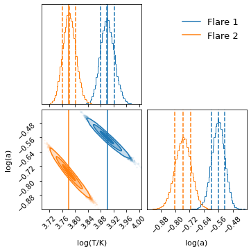
Figure 6: Posterior probability distribution for both flare samples: The sample of Flare 1 is represented in blue and the samples of Flare 2 are in orange. The sampling is done in logarithmic parameter space such that both the temperature $T$ and the area parameter $a$ are given here in logarithmic scale.

4.2 Flare temperature by epoch

The flare temperature was calculated epoch-by-epoch to acquire the time evolution of the color temperature, see Figure 7. Thus, fluxes were computed for every time step and compared with each other as presented in Section 3.2.

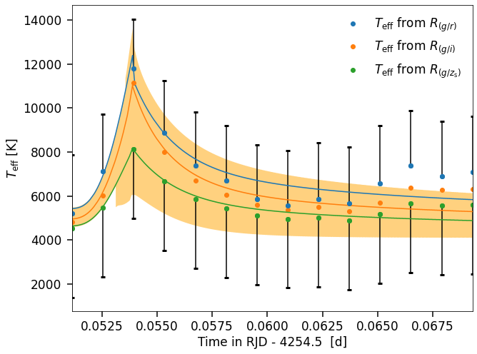
Figure 7: Temperature evolution of Flare 1: Using the ratio functions $R_{j}$, we infer for each time step a flare color temperature by comparing the observed flux ratios with the theoretical black body flux ratios in between two MuSCAT filters using the $\chi^{2}$ method. Different ratio functions $R_{j}$ yield different temperature evolutions. The uncertainty range is indicated by black markers and is valid for all three temperature evolutions. The lines represent the smoothly varying model for the flare color temperature which is derived from the best-fit parameters of the MCMC fitting to the flare light curve using the flare template aflare1. The orange shaded area gives the overlaid uncertainty of all three models.

Because the observations in different passbands yield different cadences, we had to bin the observed flux to compare the theoretical black body fluxes between two filters. The uncertainty in each time step was propagated from the uncertainty of the filter-specific fluxes to the ratio functions.

To obtain a smoothly varying model for our epoch-by-epoch color temperature, we made use of our best-fit flare flux profile model. We fit the flare template aflare1 to the flare flux profile for each flare and MuSCAT passband, obtaining a smooth flux model for the flare event. Subsequently, we performed the same steps as before to retrieve the color temperatures from these flux profiles, cf. Section 3.2. We used our color temperature model to compute the global flare temperature, cf. Section 4.3.

4.3 Global vs peak flare temperature

If signal-to-noise ratio (S/N) is low, the temperature evolution is not a precise measure for the color temperature of the flare and other measures should be used (Namekata et al., 2020). A more sophisticated approach to determining the temperature of a given flare makes use of the total instead of the epoch-by-epoch flux. Using our best-fit approximation for the flare flux profile (see Section 3.3), we calculated the total flux in each filter by integrating the flare template aflare1 with our best-fit parameters obtained for each flare. We compared the acquired flux ratios for each filter pair and applied the ratio functions $R_{j}$ to yield an estimate of the ratio-specific global flare temperature. The same can be done for the peak fluxes that is, the flux within the FWHM of the flare. Table 2 shows the global and the peak flare temperatures, respectively, for every possible filter combination in comparison to the derived SED temperatures. Also, we combined our results for all filters by weighting the temperatures by their uncertainties.

Table 1: Flaring area parameter and respective flaring areas for both flares shown in fractional units of the stellar radius.

Global	Fraction of $R_{\mathrm{star}}$
	$\text{a}\times R_{\mathrm{star}}$	$\text{A}\times\pi R_{\mathrm{star}}^{2}$
Flare 1	$0.266\begin{subarray}{c}+0.023\\ -0.021\end{subarray}$	$0.071\begin{subarray}{c}+0.001\\ -0.001\end{subarray}$
Flare 2	$0.171\begin{subarray}{c}+0.019\\ -0.017\end{subarray}$	$0.029\begin{subarray}{c}+0.001\\ -0.001\end{subarray}$
Peak	Fraction of $R_{\mathrm{star}}$
	$\text{a}\times R_{\mathrm{star}}$	$\text{A}\times\pi R_{\mathrm{star}}^{2}$
Flare 1	$0.536\begin{subarray}{c}+0.062\\ -0.070\end{subarray}$	$0.288\begin{subarray}{c}+0.004\\ -0.005\end{subarray}$
Flare 2	$0.213\begin{subarray}{c}+0.027\\ -0.031\end{subarray}$	$0.045\begin{subarray}{c}+0.001\\ -0.001\end{subarray}$

Table 2: Global and peak flare temperatures retrieved from the observation of the two TRAPPIST-1 flares.

	Global $T_{\mathrm{glob}}$ [K]
Ratio	Flare 1	Flare 2
$R_{(g,r)}$	$7000\pm 2500$	$6200\pm 2100$
$R_{(g,i)}$	$6300\pm 3100$	$5700\pm 2600$
$R_{(g,z_{\mathrm{s}})}$	$5600\pm 3300$	$5100\pm 2800$
Weighted Sum	$6450\pm 650$	$5800\pm 500$
From SED	$7940\begin{subarray}{c}+430\\ -390\end{subarray}$	$6030\begin{subarray}{c}+300\\ -270\end{subarray}$
	Peak $T_{\mathrm{peak}}$ [K]
Ratio	Flare 1	Flare 2
$R_{(g,r)}$	$11800\pm 2300$	$8420\pm 1880$
$R_{(g,i)}$	$11200\pm 3100$	$7350\pm 2600$
$R_{(g,z_{\mathrm{s}})}$	$8200\pm 3250$	$6300\pm 2600$
Weighted Sum	$10800\pm 1550$	$7650\pm 900$
From SED	$13620\begin{subarray}{c}+1520\\ -1220\end{subarray}$	$8290\begin{subarray}{c}+660\\ -550\end{subarray}$

The global flare temperatures take the total flux into account, whereas the peak flare temperatures are calculated using the flux within the FWHM. For comparison, the temperatures inferred from the SED of the individual flares are also shown.

5 Discussion

Flare temperatures on active M-dwarf stars (dM3e-dM4.5e) were previously derived from spectroscopic and photometric observations (Kowalski et al., 2013; Johnson et al., 2021) - $T_{\mathrm{glob}}=9000-10000$ K and $T_{\mathrm{peak}}=9000-14000$ K. It is usually assumed that flares on ultra-cool dwarfs have similar temperatures (e.g. Kowalski et al., 2013; Paudel et al., 2018; Günther et al., 2020; Glazier et al., 2020, and references therein). In this work, we showed with real photometric data that this assumption cannot be transferred to TRAPPIST-1, an ultra-cool M-dwarf with spectral type M7.5V. Thus raises the question of whether or not flares on late M-dwarfs should in general be modeled with cooler temperatures than early M-dwarfs.

5.1 SED versus two-filter method

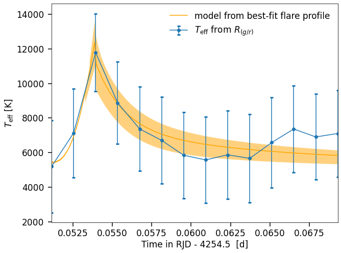
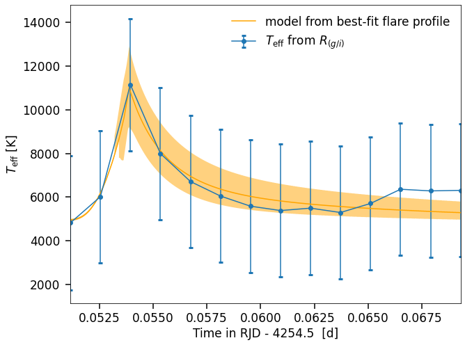
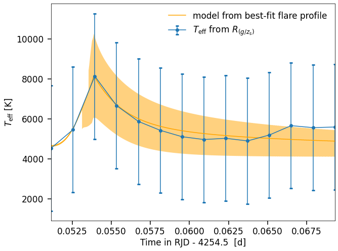
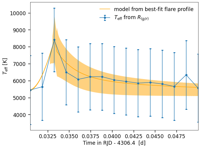
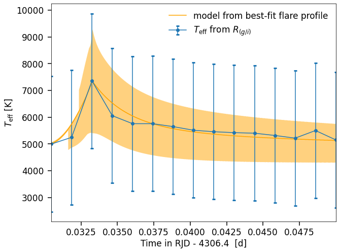
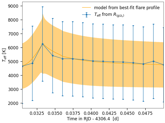
Figure 17: Color-temperature evolution for both observed TRAPPIST-1 flare with MuSCAT 2. In the left column, all temperature evolutions for the different filter ratio functions $R_{j}(T_{\mathrm{eff}})$ are shown, and in the right column, the same is done for flare 2. The orange line indicates the model drawn from the best-fit to the flare flux profile, with respective model uncertainties represented by the orange shaded areas.

The results from both the SED and the two-filter method imply that the global and peak temperature for the observed TRAPPIST-1 flares are lower than expected from the empirical flare temperatures used in modeling the energy budget of a flare (e.g. Segura et al., 2010; Kowalski et al., 2013; Tilley et al., 2019; Howard et al., 2020, and references therein), except for the peak temperature of Flare 1, where the temperature from both applied methods is consistent with the literature. The two methods are consistent within a $2-\sigma-$confidence interval; see Table 2 for Details. The color temperature evolutions are shown in Figure 7 and Figure 17. For both flares, the different ratio functions are consistent within the uncertainties. Comparing both methods, the clear advantage of the SED method is the simultaneous use of all filter fluxes and the simultaneous fit of the area parameter. As a consequence, the SED method is not affected by the disadvantage that we do not have a blue filter in our data set. The uncertainties on the two-filter methods could be improved by MCMC sampling of the theoretical black body flux values rather than using a simple $\chi^{2}$ reduction. However, this is beyond the scope of this paper as the two-filter method was only meant to prove the temperature consistency of our SED method.

For Flare 1, the peak temperature for both applied methods is between 9000 and 14000 K and is therefore consistent with the literature. For Flare 2, the peak temperature lies within 2-$\sigma$ from the literature value for both methods. The reason for these consistent peak temperatures could be twofold. The fitting of the temperatures becomes more difficult toward higher temperatures because of the lack of a bluer photometric filter. This is partly monitored by the larger uncertainties that we obtain for the peak SED temperatures in comparison to the global SED temperatures. On the other hand, if the flare has high peak SED temperatures but lower global SED temperatures, this could imply that the cooling mechanisms are different in the atmosphere TRAPPIST-1 in comparison to earlier M-dwarfs.

5.2 SED temperature uncertainties

For the SED method, the estimated uncertainties were inferred by Gaussian uncertainty propagation taking the uncertainty from the flare flux profile and the uncertainty on the mega-MUSCLES spectrum. The marginalized uncertainties on the temperature were estimated directly by taking the $84^{\mathrm{th}}$ and 16^th percentiles of the MCMC samples. Observing Figure 5 closely, the uncertainties on the $z_{\mathrm{s}}$-flux are the largest, extending over the whole SED flux regime for Flare 2. The $z_{\mathrm{s}}$-flux is more sensitive to the flux-profile-fitting component, because of the low flare S/N in the $z_{\mathrm{s}}$-band. For Flare 2 the low S/N prevented an accurate fit to the flare flux profile in the $z_{\mathrm{s}}$-band and therefore we obtain large uncertainties.

Strong emission lines can also contribute to uncertainties. For instance, the peak flare flux could be contaminated by H$\alpha$ and H$\beta$ emission by up to 10$\%$ and 8.8$\%$ of the total flux (Kowalski et al., 2013), respectively. Taking the maximum of the H$\alpha$ contribution into account, the $r$-filter flux was reduced for the global calculation and for the peak calculation by roughly $30\%$ and $26\%$, respectively. Indeed, this correction for the H$\alpha$ contribution results in higher flare temperatures because the $r$-filter flux is corrected toward lower flux values, meaning that the SED is more likely to be fit with higher temperatures, unless another line contamination is considered. This could be compensated by the H$\beta$ emission in the $g$-filter. We reduced the flux in $g$-filter by approximatly $50\%$ and $20\%$ for the total and peak calculations, respectively. As a consequence of the flux reduction in the $g$-filter the overall shape of the SED is shallower for both cases such that it is more likely to fit with lower temperatures than that of the reported black body. Contamination from both lines is probably is present in our data and therefore they will cancel each other out to a certain degree. However, it is impossible to correct the SED for the real H$\alpha$ and H$\beta$ contributions. By omitting line emission in our calculations our uncertainties on the inferred black body temperatures are increased, but also it does not indicate a clear bias since the strongest line emission are prone to cancel each other out to a certain degree in the fitting procedure

5.3 Flare location

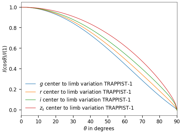
Figure 18: Center-to-limb variation for the MuSCAT filters. The limb darkening is modeled with quadratic law (Claret 2000).

The position of the flare on the stellar surface has an impact on the received flux and therefore might alter the SED. Because of the rotation of TRAPPIST-1 with period $P\in[1.4,3.295]$ days (Gillon et al., 2016; Vida et al., 2017; Luger et al., 2017), the flare might move over the stellar surface during its emission. The observed flares have durations of less than 30 minutes and therefore their angular movement on the surface is $\Delta\alpha\in[4.5,1.9]^{\circ}$. The projected angles are even smaller, such that the time was not sufficient for the observed flares to move from the limb to the center or vice versa. Thus, we assumed that the projected surface area of TRAPPIST-1 is constant. Applying simple laws of limb darkening (Claret, 2000), it was evident that the flux at the limbs reduced already at a line-of-sight angle of roughly 60 degrees to half its value at the center. Because the M2 data are given in relative units we used the mega-MUSCLES Spectra for TRAPPIST-1 to derive the SED of the flare. Bluer colors are more affected by limb darkening; see Figure (18) of the Appendix. As discussed in Section 5.4, the flare temperature determines the slope of the SED and therefore the reduction of the flux close to the limb can be neglected. If we assume that the flares occurred close to the limb, the shape of the SED would result in a higher temperature than if they occurred in the vicinity of the center; see Figure 18. Therefore, we assumed that our best-fit temperatures are consistent with lower temperatures and independent of the exact position on the stellar surface.

5.4 Black body model

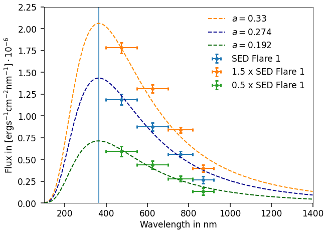
Figure 19: Model sensitivity test for the flare area parameter: three SEDs are shown for Flare 1. The blue SED indicates the SED with absolute calibration to Gaia and the orange and green curves represent fluxes with altered SEDs.

Our model relies on two main characterizing parameters, the flare temperature $T_{\mathrm{eff}}$ and the flare area parameter $a$; see Section C.1 in the Appendix. The black body distribution determines the shape and slope of the model. Here, $a$ is the constant of proportionality between the observed flux and our model. Using the MuSCAT data directly, the flare area parameter would not be a measure for the real covered radius fraction, because the MuSCAT data are given in relative units. We therefore calibrated our observation to the Gaia absolute fluxes. Qualitatively, the flare area parameter shows the expected behavior. Flare 1 emits more flux and therefore has also a larger flare area parameter than Flare 2. Because the flare temperature is the parameter that determines the shape of the SED, our model can still determine $T_{\mathrm{eff}}$ satisfactorily even if no absolute calibration is done but only the relative MuSCAT calibration. We tested this behavior for both flares obtaining the same temperatures but different flaring area parameters. Also, we performed a model sensitivity test for Flare 1 by multiplying the flare flux by arbitrary constant factors; see Figure 19. Multiplying the SED with constant factors resulted in a change in the flare area parameter but left the temperatures unchanged.

5.5 Residuals in flare profiles

In Figure 4 the fit shows residual systematic errors. This could be due to complex flare events with multiple peaks or QPPs. Any superimposed flare would increase flux. As discussed in the previous section, the amount of flux is regulated by the flare area parameter and therefore a superimposed flare would not contaminate our flare temperatures, unless it changes the shape of the SED. Additionally, we employed a sinusoidal fit to the residuals with period $P=29.02\pm 6.53$ min. Typical durations for QPPs range from several seconds to tens of minutes for M-dwarf flares (e.g Van Doorsselaere et al., 2016; Million et al., 2021). Because our period is consistent with the typical QPP periods we considered our systematic errors to be explained by a QPP. The flux oscillations do not imply the flare temperatures and therefore the main result of our paper remains valid. For this reason, we neglected the observed QPP for our calculations.

5.6 Flare temperatures per spectral type

Figure 8 shows the flare continuum temperatures for TRAPPIST-1 and other M- and L-dwarfs from different photometric and spectroscopic studies (Mochnacki & Zirin, 1980; Hawley & Pettersen, 1991; Kowalski et al., 2013; Gizis et al., 2013; Howard et al., 2020). The upper panel reveals a possible trend for low-mass stars. The hottest flares seem to get cooler toward lower masses, such that the higher right corner is not populated by flares. This could be explained by a selection bias. As Howard et al. (2020) pointed out in their energy-temperature relation, more energetic flares seem to be hotter; see Figure 9. These higher energetic flares are more likely for earlier type M-dwarfs (Howard et al., 2019; Günther et al., 2020) and therefore hotter flare temperatures $T_{\mathrm{eff}}>10000$ K could be caught more frequently for early M-dwarfs than for later types like TRAPPIST-1.

Toward the tail of the low-mass-stars, there are only three flare temperatures measured. All three of them have bolometric flare energies between $10^{31}$ and $10^{32}$ and are in the lower energy tail of the energy-temperature relation. Therefore, it is difficult to verify the trend with spectral type, as there are not yet enough measurements of ultra-cool dwarf flares. Later type stars turn fully convective at roughly spectral type M4V and have cooler atmospheres, i.e. surface temperatures of below $T_{\mathrm{eff}}=3200$ K (Chabrier & Baraffe, 1997; Reid & Hawley, 2013). If the trend with spectral type is physical it might be due to a different flare generation process for fully convective stars in comparison to stars with radiative cores. Also, the heating mechanisms of the lower chromosphere driven by the accelerated particles could be different in late M-dwarfs. Without further observation and modeling of ultra-cool M-dwarf chromospheres, this discussion remains speculative.

Figure 9 shows the energy-temperature relation including the two TRAPPIST-1 flares for bolometric energies. We fit a power law of the form $\log_{10}(T_{\mathrm{eff}})=\alpha\cdot E_{bol}+\beta$ with two coefficients $\alpha$ and $\beta$ to the Howard et al. (2020) sample, including the two TRAPPIST-1 flares, and obtain for the total temperatures $\alpha_{tot}=(6.98\pm 0.03)\cdot 10^{-2},\beta_{tot}=1.5\pm 0.4$ and for the peak temperatures $\alpha_{peak}=(9.67\pm 6)\cdot 10^{-2},\beta_{peak}=0.8\pm 0.7$ . Both peak and global temperatures of the TRAPPIST-1 flares are consistent with the uncertainty of the relation. However, we argue that the correlation is complete only if the flaring area is included in the relation because we expect that the heating process is affected not only by the energy released from the magnetic field but also by the size of the area that is heated. This could explain the large observed scatter especially for the peak temperatures. To obtain a correlation between energy-temperature and area, we propose to measure area and temperature simultaneously and dependent on each other in future similar studies; for example, by taking the dominant cooling mechanism in the chromosphere we could model how the temperature is distributed at the flare footpoints and how the area evolves then with time in dependence of the temperature. However, this is beyond the scope of the present work.

From the density map in the lower panel of Figure 8, it follows that cool flares $T_{\mathrm{eff}}<8000$ K are also present in early spectral types and are not exclusively occurring on late M-dwarfs. Nevertheless, it appears that they are less frequent than flare temperatures around $T_{\mathrm{eff}}=10000$ K. Following the energy-temperature relation, surprisingly, lower flare temperatures are not denser on the map, as they should occur more frequently. This could be explained by selection effects due to observational limitation for example.

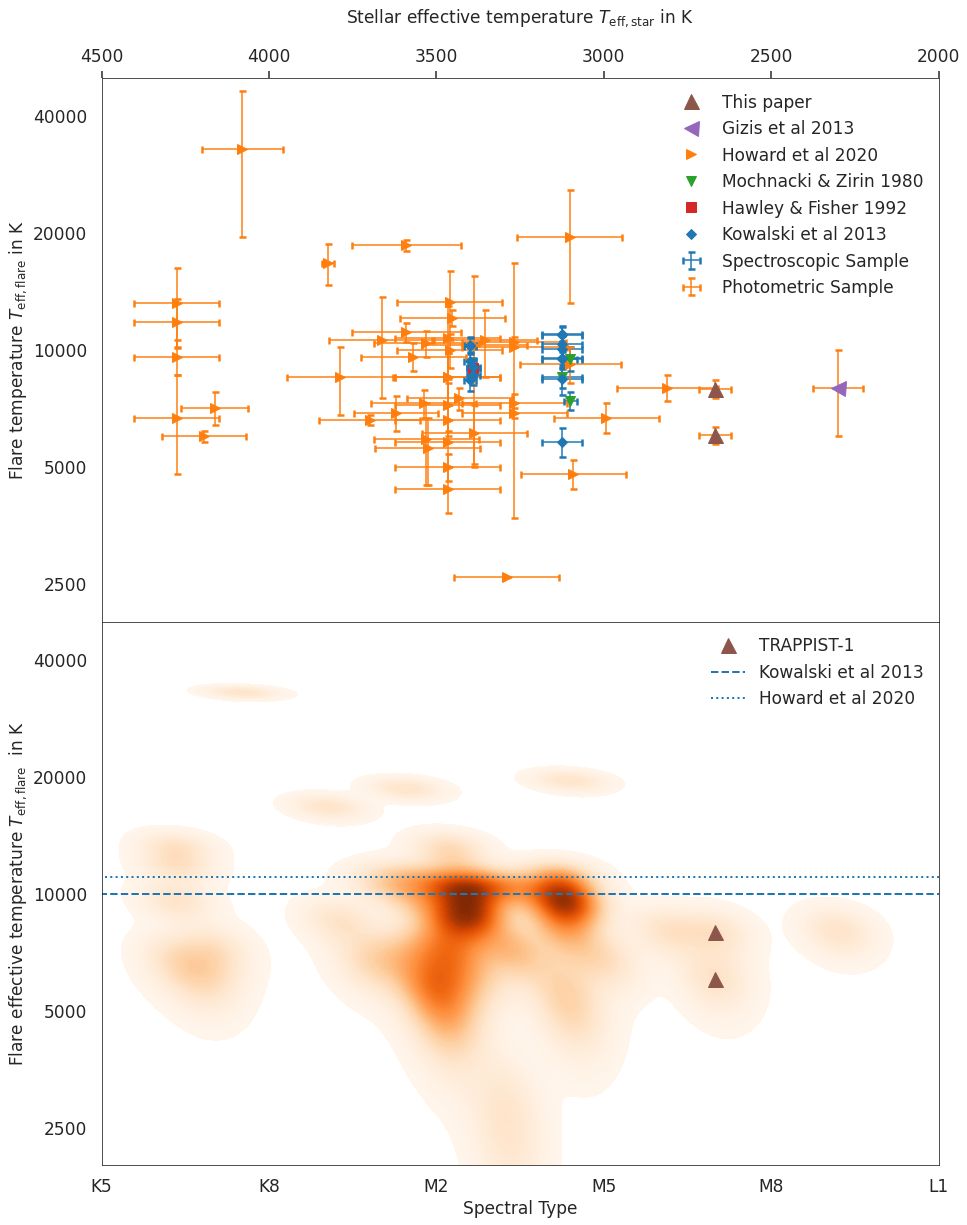
Figure 8: Spectral type and stellar effective temperature versus total flare temperature for different photometric and spectroscopic studies: The upper panel uses the stellar effective temperature if available from the TESS input catalogue (Stassun et al., 2019). For the Kowalski sample, we use conservative uncertainties of $\pm 500$K. The lower panel shows a density map of flare temperatures per spectral type that is consistent with the upper stellar effective temperatures. The flare temperature axis is represented in log-scale. The two TRAPPIST-1 flares are overplotted and the blue horizontal lines represent the average temperatures from the two biggest temperature samples.

Figure 9: Energy-temperature relation in log-log representation: In the upper panel the global flare temperatures are plotted versus the bolometric energy, whereas in the lower panel the peak temperatures are used. The flares from Howard et al. (2020) are indicated in blue and our two TRAPPIST-1 flares are shown in orange. The blue dashed line indicates a power-law fit to the data.

Figure 10 a histogram of measured total temperatures from the same sample as in Figure 8. The distribution reveals the peak at 10000 K as expected. Our TRAPPIST-1 flares with 6030 and 7940 K, respectively, seem less likely but not at all unlikely. The histogram shows that the numbers of flares in a given temperature range increase, until 11000 K is reached. Afterwards, there appears to be a cut. Between 11000 and 12000 K the observed numbers decrease strongly. It appears that flares with $T_{\mathrm{eff}}=10000-11000$ K are the most likely observed ones and flares with temperatures below 10000 K appear to be more likely than flares with $T_{\mathrm{eff}}>11000$ K. This could be explained by the empirical energy-temperature relation mentioned above. Flares with higher energy are less likely to occur and therefore also flares with higher temperatures are less frequent.

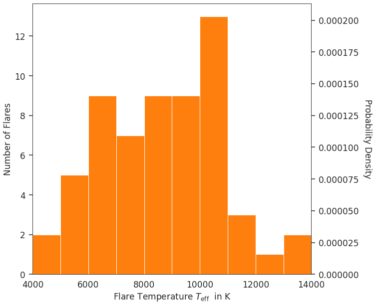
Figure 10: Histogram of total flare temperatures from the spectroscopic and photometric observations shown in Figure 8 with the peak of the distribution close to 10000 K.

Taking the energy-temperature relation and the flare frequency distribution (FFD; see following Section), we predict that we would have to observe TRAPPIST-1 for at least 15 days to find a flare with temperatures above 10000 K. Taking this into account, we conclude that the flares observed on TRAPPIST-1 show lower temperatures than expected when compared to the average temperatures from previous studies (Hawley et al., 2003; Shibayama et al., 2013; Kowalski et al., 2013; Howard et al., 2020). However, if the flare frequency distribution and the energy-temperature relation are considered it is not surprising that we observed lower flare temperatures for TRAPPIST-1.

5.7 Flare frequency distribution and habitability

One goal of our analysis was to update the FFD of TRAPPIST-1 (Paudel et al., 2018; Glazier et al., 2020) and show the implications of a different flare temperature. The FFD is the cumulative rate of flares per time unit (Gershberg, 1972) and is frequently described by a power law (Davenport, 2016; Paudel et al., 2018; Günther et al., 2020; Glazier et al., 2020). In log-log space, this power law has a linear appearance,

$$\log_{10}{\nu}=\alpha\log_{10}{E_{\mathrm{bol}}}+\beta,$$ (4)

where $\nu$ is the occurrence rate of the flares in a given time unit, $E_{\mathrm{bol}}$ is the bolometric energy $\alpha$ indicates the slope and $\beta$ is the y-intercept in log-log space. The bolometric energies were calculated as presented in Section B.3 of the Appendix and we adopted a value of 7000 $\pm 500$ K for the flare temperature, which is consistent with the results of this paper.

First, we took the flares found by Paudel et al. (2018) in the K2 light curve and computed the bolometric energies by adopting their $ED$s following Section B.3.

The updated FFD for the combined information of M1, M2 and K2 is shown in Figure 11. We observe a truncated power law with a turnoff at roughly $10^{30}\mathrm{erg}$. This is a result of flares with lower energies close to the K2 detection limit as discussed for Kepler by Hawley et al. (2014). The theoretical detection limit for M2, shown by the vertical dashed line, is given by the $g$-band; see Section 3.1. The orange squares indicate the two M2 flares, while the black points represent the K2 flares (Paudel et al., 2018).

Using the power law ansatz for the flare frequency equation (4), we fit the flare frequency with the MCMC approach of Wheatland (2005) implemented in AltaiPony. The best-fit to the data is indicated by the red solid line, as well as 100 samples of the 2500 MC trials. By extrapolating the FFD to larger bolometric energies, we explored the FFD into the regime of low flare occurrence, that is higher energies. We analyzed potential danger to the atmospheres of the TRAPPIST-1-companions and possible abiogenesis. The blue dash-dotted line indicates the best-fit if the bolometric energies were calculated with a black body temperature of 10000 K. Comparing the two best-fit solutions with the different adopted temperatures, we obtained $\alpha_{7000\mathrm{K}}1.45\pm 0.20$ , $\alpha_{10000\mathrm{K}}=1.46\pm 0.24$. The higher temperature led to a slightly steeper slope. However, the impact is not significant because both slopes are consistent with each other. In the abiogenesis zone of an MS star, specific prebiotic chemical reactions are possible that enable the synthesis of ribonucleic acid (RNA) (Rimmer et al., 2018; Günther et al., 2020). The flare frequency $\nu$ needed to trigger and sustain prebiotic chemistry is given by Günther et al. (2020);

$$\nu\geq 25.5\hskip 2.84544pt\mathrm{days}^{-1}\left(\frac{10^{34}\mathrm{erg}}{{E_{\mathrm{U}}}}\right)\left(\frac{R_{\mathrm{star}}}{R_{\odot}}\right)^{2}\left(\frac{T_{\mathrm{star}}}{T_{\odot}}\right)^{4}$$ (5)

where $E_{\mathrm{U}}$ is the U-band energy, $R_{\mathrm{star}}$ the stellar radius and $T_{\mathrm{star}}$ the stellar surface temperature. In Figure 11, the abiogenesis zone is plotted in green, adopting the surface temperature and radius of TRAPPIST-1 of $T=2648\pm 26$ K (Wilson et al., 2021) and $R=0.1192\pm 0.0013$ $R_{\odot}$ (Agol et al., 2021). Both the red and blue lines do not intersect with the abiogenesis zone, indicating, that the high energetic flux from TRAPPIST-1 flares is likely to be insufficient to trigger and sustain prebiotic chemistry. Glazier et al. (2020) came to the same conclusion.

The yellow shaded area in Figure 11 marks the ozone depletion zone around TRAPPIST-1, where frequent high-energy flares may erode exoplanet atmospheres and lead to subsequent surface sterilization. Tilley et al. (2019) modeled the impact of M-dwarf flares on the atmosphere of an Earth analog planet. These authors argued that Earth’s ozone layer should erode if flares with bolometric energies $\geq 10^{34}$ erg hit the atmosphere at a frequency of $\nu_{34}\geq 0.4\hskip 2.84526pt\text{day}^{-1}$. Günther et al. (2020) gave a lower limit for the frequency $\nu_{34}\geq 0.1\hskip 2.84526pt\text{day}^{-1}$. We adopted the more conservative approach of Günther et al. (2020), which also allowed us to remain consistent with the analysis of Glazier et al. (2020). As the best-fit did not intersect with the ozone-depletion zone, we conclude that the UV flux is insufficient to deplete a complete Earth-like ozone layer.

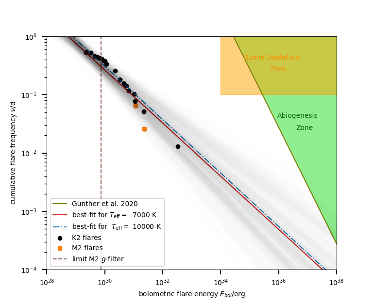
Figure 11: Flare frequency distribution for K2 and M2 data. The FFD for TRAPPIST-1 is updated by our flares indicated in orange. The black points are adopted from (Paudel et al., 2018). The best fit to the power law is chosen from 2500 MC trials, here only 100 random samples are shown to mark the uncertainty of the model. Also overplotted are the abiogenesis zone in green (Rimmer et al., 2018; Günther et al., 2020) and the ozone-depletion zone in yellow (Tilley et al., 2019; Günther et al., 2020) for TRAPPIST-1.

6 Conclusion

We used 59 nights of multi-color photometric observations of MuSCAT1 and MuSCAT2 to search for flares on TRAPPIST-1. We found two flares in the MuSCAT2 light curves. Moreover, we discovered that the black body temperatures associated with the total emitted flux are likely to be cooler than previously suggested for ultra-cool M-dwarfs. We inferred temperatures of $T_{\mathrm{SED}}=7940\begin{subarray}{c}+430\\ -390\end{subarray}$ K for Flare 1 and $T_{\mathrm{SED}}=6030\begin{subarray}{c}+300\\ -270\end{subarray}$ K for Flare 2. We obtained peak temperatures $T_{\mathrm{SEDp}}=13620\begin{subarray}{c}+1520\\ -1220\end{subarray}$ K for Flare 1 and $T_{\mathrm{SEDp}}=8300\begin{subarray}{c}+660\\ -550\end{subarray}$ for Flare 2. The observed peak black body temperatures for TRAPPIST-1 also show marginally cooler temperatures for Flare 2, while they are consistent with the literature for Flare 1. It could be that different cooling mechanisms in the stellar atmosphere are responsible for this behavior and that cooling is more efficient toward later spectral types. This remains speculative without further spectroscopic measurements and modeling. Lower black body temperatures for flares lead to different UV surface fluxes and therefore have an impact on the habitability estimation on exoplanets around ultra-cool M-dwarfs, even though we showed the bolometric energies remain marginally affected. While using the 9000-10000 K assumption one has to keep in mind, that flares with lower temperatures are more likely to occur and thus, we suggest using a flare frequency temperature distribution to account for the different flare temperatures in the future.

Furthermore, we conclude that, based on our data, it is not possible to verify whether the lower observed temperatures on TRAPPIST-1 are intrinsic to ultra-cool dwarfs or are the result of lower energies generated for these late-type stars, making it more likely to observe lower flare temperatures as suggested by the energy-temperature relation. Our prediction of roughly 15 days of observation to observe a flare with $T_{\mathrm{eff}}>10000$ K is a considerable task for future work and would also show whether or not the energy-temperature relation can be expanded to the low-mass end of M-dwarfs.

Our SED method proves to be suitable for estimating flare temperatures and areas. It is a good trade-off between previous multi-color photometric- and spectroscopic approaches because of its efficiency and low cost. Even though spectroscopic methods enable the resolution of the specific line emission, we show that our model allows us to infer precise temperatures and areas associated with stellar flares.

Further multi-color observations are needed to put constraints on other M-dwarf flares in order to verify whether or not the observed behavior is indeed a general characteristic of ultra-cool M-dwarfs. The reported trend of lower flare temperatures toward later spectral types could be investigated by a thorough observation campaign of several late M-dwarfs and early L-dwarfs to populate the low-mass tail in Figure 8. M-dwarfs with a surface temperature of $\sim 3000$ K are particularly suitable targets as they show enhanced activity in comparison to other M-dwarfs and earlier type stars (Günther et al., 2020). We recommend temperature measurements of similar stellar types to TRAPPIST-1 with bluer filters. Also, we encourage the spectroscopic observation of ultra-cool M-dwarf flares in order to infer H$\alpha$ and H$\beta$ contributions, for example, to improve the results.

Appendix A Flare detection limits of the MuSCAT 2 instrument

Table 3: Observation of TRAPPIST-1 for the different instruments.

Instrument	Total Time [d]	Cadence [s]
M1	(1.2, 0.8, 0.2)	(85, 64, 68) $z_{\mathrm{s}}$,$r$,$g$
M2	(4.2, 3.4, 4.5, 4.2)	(39, 60, 63, 61) $z_{\mathrm{s}}$,$i$,$r$,$g$
K2	75	60

Shown are the total observation time and the cadence for each instrument. The cadence is averaged over the whole observation period of the respective instrument. We note that for the MuSCAT instruments the cadence varies strongly in each observation year such that the average should be understood as a rough estimation. We have an observation in 2016 for K2, 2016, 2017 and 2020 for M1 and 2017, 2018, 2019 and 2020 M2.

To infer the detection limits, we generated a mock light curve, for each M2 filter by adopting normalized flux and adding Gaussian noise with a mean equal to the median of the respective noise level of all M2 observations for TRAPPIST-1. The typical observation time is calculated from Table 3 by adapting the total observation time per filter and their averaged cadences. The results from FLIR are shown in Figure 12, where the injection of 20000 classical single-peaked events with the Davenport et al. (2014) template aflare1 were visualized for each filter. The FLIR was executed iteratively, i.e. only one flare was injected per iteration in the light curve to avoid overlapping of injected flares. In Figure 12, the dark regions mark low recovery probability, while the yellow areas indicate high recovery probability .

We defined the detection limit as the region where the FLIR delivers $100\%$ recovery probability, for the first time, because there we were certain that any flare event with these properties would be detected. This approach may seem too conservative but as the light curve is artificial, it seems appropriate to remain as conservative as possible. The detection limits in terms of bolometric energy, FWHM, and amplitude of the flare are listed in Table 4. The ranges for FWHM and amplitude implied that the recovery probability was calculated in FWHM and amplitude bins, such that in the given bin with the border of the given ranges, we have $100\%$ recovery probability. The bolometric energy was then calculated using the central value of these ranges by adopting the equations presented in Section B.3, where the uncertainty was computed by Gaussian error propagation and is constrained by the width of the FWHM and the amplitude for a given filter.

Table 4: The lower detection limits for MuSCAT.

Filter	FWHM [$\mathrm{min}$]	Amplitude	$E_{\mathrm{bol}}$ [$10^{30}\mathrm{erg}$]
$g$	$[5.4,5.76]$	$[0.059,0.075]$	$0.74\pm 0.05$
$r$	$[4.32,4.68]$	$[0.03,0.04]$	$3.12\pm 0.18$
$i$	$[3.96,4.32]$	$[0.035,0.053]$	$8.13\pm 0.45$
$z_{\mathrm{s}}$	$[2.02,2.16]$	$[0.04,0.05]$	$8.48\pm 0.81$

The lower detection limits in FWHM and amplitude for all filters associated with the bolometric energy adopting a blackbody temperature of 7000 K. Even though the adopted photometric scatter is lower in $z_{s}$ and $i$, the detection limits in $g$ and $r$ are lower in terms of energy, because the flare flux from a 7000 K is peaked closer to the blue than the red light.

We also had a limit for the detection of long-duration and hence high-energy flares. If the FWHM of the flare exceeds the duration of the observation (1.5-2 hours), the flare was not completely resolvable and the fitting process might not converge as described in Section 3.3. However, this limit was difficult to quantify because of its multidimensionality. It depends not only on the FWHM of the flare but also on its peak time and was therefore not quantified in this work. Moreover, the detection of such highly energetic flares was unlikely in our data set. By looking at the FFD of TRAPPIST-1 we identify that flares with bolometric energy of $E_{\mathrm{bol}}>10^{34}$ occur only once in 100 days. As our total observation time is roughly 5 days with the combined MuSCAT observation we neglected the detection limit of long-duration flares.

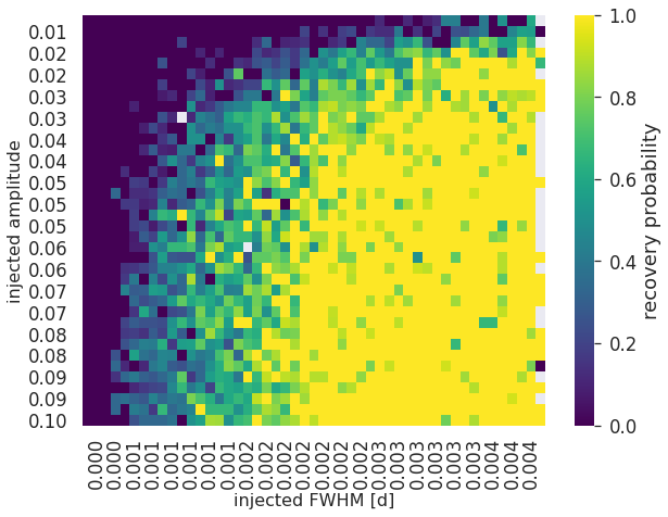
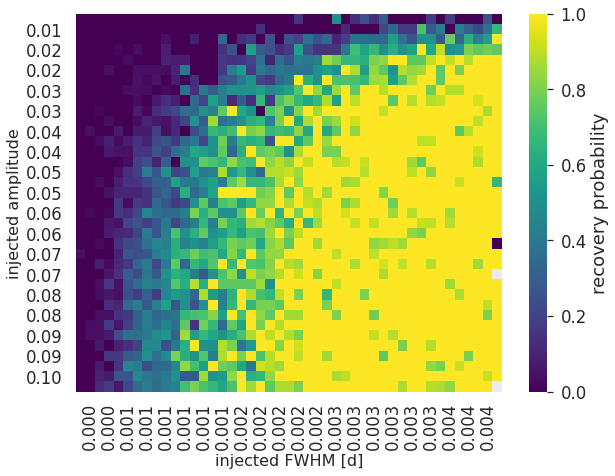
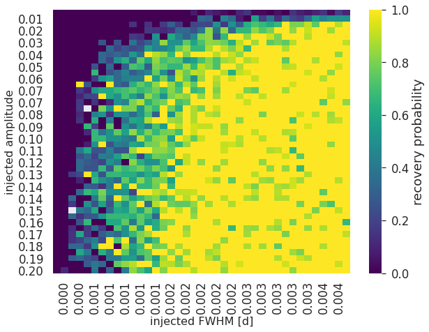
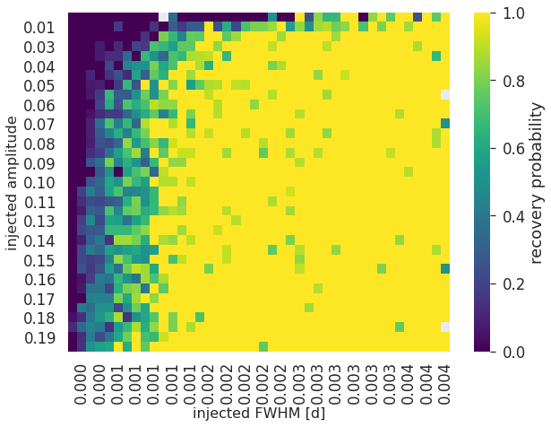
Figure 12: Flare injection recovery via heat maps for each MuSCAT 2 (M2) filter, Panels (a),(b),(c), and (d) correspond to the M2 $g$, $r$, $i$ and $z_{s}$ photometric filters. The detection limits in amplitude and FWHM of the flares are for all bands visible and marked by the dark regions where the recovery probability is low.

Appendix B Flare energetics

B.1 Analytic flare template

Davenport et al. (2014) used for the generation of their flare template aflare1 flares that occurred on GJ1243 (M4.0Ve). The duration of used flares for the generation of the template was in the range of 20-75 minutes. Therefore, both of our observed flares with durations of over $t>30$ min fit well in the selected flare range. The analytic formula for the flare flux profiles relies on a combination of polynomial and exponential fits. The rise phase, i.e., $-1t_{1/2}\leq t\leq 0$, is described by a polynomial function (Davenport et al. 2014):

$$F_{\mathrm{rise}}=1+1.941(\pm 0.008)t_{1/2}-0.175(\pm 0.032)t^{2}_{1/2}$$ (6)

$$-2.246(\pm 0.039)t^{3}_{1/2}-1.125(\pm 0.016)t^{4}_{1/2}$$

with $t_{1/2}=x-t_{\mathrm{peak}}/FWHM$ being the full width in time at the maximum of the flare and $x$ the observational time (Kowalski et al. 2013). The decay phase, i.e., $t>0$, is described by (Davenport et al. 2014):

$$F_{\mathrm{decay}}=0.6890(\pm 0.0008)e^{-1.600(\pm 0.003)t_{1/2}}+$$ (7)

$$0.3030(\pm 0.0009)e^{-0.2783(\pm 0.0007)t_{1/2}}$$

Therefore the full template reads:

$$F_{\mathrm{flare}}=(F_{\mathrm{rise}}+F_{\mathrm{decay}})\cdot|ampl|$$ (8)

where $ampl$ is the amplitude in the flux of the flare.

B.2 Gaussian prior probability

For the MCMC fitting of the flare flux profiles, we needed to define prior probability distributions for the three parameters of the flare template aflare1. The estimate of the amplitude $am_{\mathrm{rec}}$ from AltaiPony was taken as the mean of the respective Gaussian prior and $0.05$ in terms of normalized flux as a conservative standard deviation. The peak time $t_{\mathrm{peak}}$ was calculated as the argmax of the normalized flux for a given flare event. We therefore chose the standard deviation of the peak time to be one data point in each observation. The $FWHM_{\mathrm{est}}$ was only approximated very roughly by dividing the duration of the flare by the arbitrary value of four. For this reason the standard deviation for the FWHM was chosen to be $1/24$ days and the prior was therefore rather uninformative. For an overview of the adapted Gaussian priors see Table 5.

Table 5: Gaussian prior for the MCMC-approach for the MuSCAT instruments.

Parameter	M1 and M2
$t_{\mathrm{peak}}$	$\mathcal{N}(t_{\mathrm{peak}},\frac{0.2}{60\cdot 24}\text{d})$
$am_{\mathrm{flare}}$	$\mathcal{N}$($am_{\mathrm{rec}},0.05$)
$FWHM_{\mathrm{flare}}$	$\mathcal{N}$($FWHM_{\mathrm{est}}$,$\frac{1}{24}\text{d})$
$T_{\mathrm{eff}}$	$\mathcal{U}(log(T_{\mathrm{eff}}),3.3,4.4\text{K})$
$a$	$\mathcal{U}(log(a),-10,0)$

$am_{\mathrm{rec}}$ refers here to the recorded amplitude given by Altaipony and is given in terms of normalized flux. We use all filters with the same standard deviations. For the MCMC-fits of the SEDs, we use uniform priors for the effective temperature $T_{\mathrm{eff}}$ and the fraction of flaring area $a$ in logarithmic space.

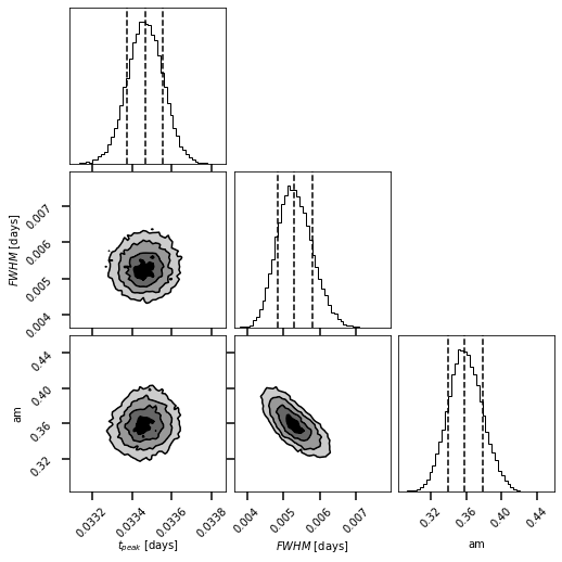
Figure 13: Corner plot of MCMC flare profile fit of Flare 2 in the $r$ passband. Shown are the correlations between the three parameters of aflare1 - peak time, full width at half maximum and amplitude. The dashed lines indicate $15^{\text{th}}$, $50^{\text{th}}$ $84^{\text{th}}$ quantiles.

B.3 Bolometric flare energies

In this chapter, we present how the flare energies were calculated. We followed the bolometric flare energy calculation of (Shibayama et al. 2013; Günther et al. 2020), where the stellar luminosity and the best-fit flare flux profile are used.

First, we calculated the bandpass independent area $A_{\mathrm{flare}}(t)$ of the flare assuming the flare luminosity can be modeled as a black body with constant effective temperature of $T_{\mathrm{flare}}=9000\pm 500$ K ,

$$A_{\mathrm{flare}}(t)=\frac{F_{\mathrm{flare}}(t)-F_{\mathrm{q}}}{F_{\mathrm{q}}}\pi R_{\mathrm{star}}^{2}\frac{\int R_{\lambda}B_{\lambda}(T_{\mathrm{eff}})d\lambda}{\int R_{\lambda}B_{\lambda}(T_{\mathrm{flare}})d\lambda}$$ (9)

where $R_{\lambda}$ denotes the instrument response function, $B_{\lambda}$ the black body radiation, $T_{\mathrm{eff}}$ the effective temperature of the star in its quiescent state, and $R_{\mathrm{star}}$ refers to the stellar radius. The effective flare temperature $T_{\mathrm{flare}}$ was chosen as a lower conservative limit in order to remain consistent with previous studies (Davenport 2016; Paudel et al. 2018; Günther et al. 2020) and references therein, but it was not a correct assumption, because the flare temperature not only changes with time but also depends on the flare phase. Also, we show in this work that the temperature associated with the whole flare event is lower than frequently adopted for ultra-cool M-dwarfs.

Having $A_{\mathrm{flare}}(t)$, we can compute the bolometric flare energy $E_{\mathrm{flare}}$ of the flare, using its corresponding luminosity,

$$E_{\mathrm{flare}}=\int L_{\mathrm{flare}}(t)dt=\sigma_{\mathrm{sb}}T_{\mathrm{flare}}^{4}\int A_{\mathrm{flare}}(t)dt$$ (10)

We calculate the uncertainties of the calculation using Gauss uncertainty propagation. Integrations of this section were performed via the trapezoidal sum rule.

B.4 Filter-specific flare energies

We calculated not only the bolometric but also the filter-specific energy, in order to infer the detection limits. We obtained the filter-specific energies by adopting a conversion constant from the bolometric energies. Assuming the flare has a bolometric luminosity $L_{\mathrm{flare}}(t)$ and filter specific luminosity $L_{\lambda,\mathrm{flare}}(t)$, then:

$$L_{\mathrm{flare}}(t)=\sigma_{\mathrm{sb}}T_{\mathrm{flare}}^{4}A_{\mathrm{flare}}(t)$$ (11)

$$L_{\lambda,\mathrm{flare}}(t)=L_{\mathrm{flare}}(t)\cdot c$$ (12)

where the flaring area $A_{\mathrm{flare}}(t)$ is not passband-specific, $T_{\mathrm{flare}}$ is the effective blackbody temperature from the flare and $c$ denotes the dimensionless conversion constant. By using $L=F\pi d^{2}$, we obtain:

$$c=\frac{L_{\lambda,\mathrm{flare}}}{L_{\mathrm{flare}}}=\frac{F_{\lambda,\mathrm{flare}}}{F_{\mathrm{flare}}}$$ (13)

with $F_{flare}$ denoting the flux from the flare event. Because the bolometric energy associated with the flares was defined as in equation (10), we derived the passband-specific energy using equation (13):

$$E_{\mathrm{flare},{\lambda}}=\int L_{\lambda,\mathrm{flare}}dt=c\int L_{\mathrm{flare}}dt$$ (14)

The calculated conversion constants for M1/M2 filters are given in Table 6.

Table 6: Conversion constants for the MuSCAT filters.

Filter	Conversion constant
$g$	0.412
$r$	0.203
$i$	0.100
$z_{\mathrm{s}}$	0.058

The constants are used to transform bolometric flare energies to passband-specific energies. We assumed here that the flare temperature is 7000 K.

Appendix C Flare temperatures

Table 7: Ratio function for different MuSCAT filters and their asymptotic limits.

Ratio	Asymptotic limit
$R_{(g,r)}$	3.18
$R_{(g,i)}$	6.94
$R_{(g,z_{\mathrm{s}})}$	12.11

Table 8: Peak S/N for both observed MuSCAT 2 flares.

	S/N
Filter	flare 1	flare 2
$g$	17.5	4.3
$r$	11.6	4.8
$i$	5.4	3.76
$z_{\mathrm{s}}$	3.4	1.6

There is a clear trend visible from higher S/N towards the bluer light for both flares.

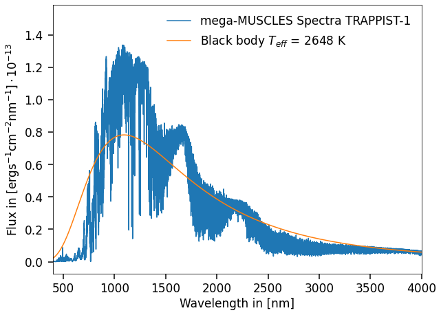
Figure 14: The semi-empirical mega-MUSCLES spectra for TRAPPIST-1 include emission and absorption lines. In comparison the black body temperature model for TRAPPIST-1 $T_{\mathrm{eff}}=2648$ K is shown.

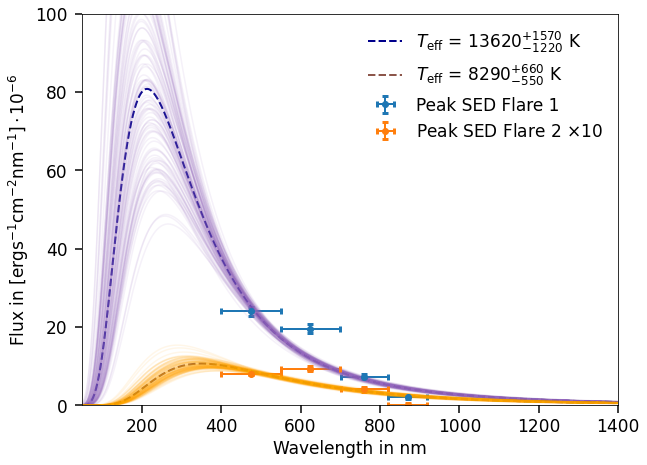
Figure 15: The SED of the peak fluxes for the two observed M2 flares. The SEDs fit with a model where the temperature $T_{\mathrm{eff}}$ was left as a free parameter using again emcee. The uncertainties of the model are indicated with 100 random samples from the chain.

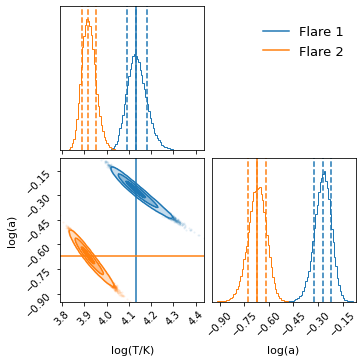
Figure 16: Posterior probability distribution for both peak flare samples: The sample of flare 1 is represented in blue and the samples of flare 2 are in orange. The sampling is done in logarithmic parameter space such that both the temperature $T$ and the area parameter $a$ are given on logarithmic scale.

C.1 Flare black body model

In this section, we show our used black body model for the fitting process described in section 3.2. We start at the apparent brightness of the observer,

$$l_{\lambda}=\frac{L_{\lambda}}{4\pi d^{2}},$$ (15)

with $L_{\lambda}$ the luminosity and $d$ the distance of the source. As the flare occurs on the visible side of the star, we integrate only the visible area from the star. Thus, we obtain

$$L_{\lambda}=4\pi^{2}R_{*}^{2}B_{\lambda}(T_{*}),$$ (16)

with $R_{*}$ the radius of the star and $B_{\lambda}(T_{*})$ the black body spectrum of temperature $T_{*}$. Substituting back in to the apparent brightness,

$$l_{\lambda}=\frac{R_{*}^{2}}{d^{2}}\cdot\frac{1}{\exp{\frac{hc}{k_{b}T_{*}\lambda}}-1}\cdot\frac{2hc^{2}}{\lambda^{5}}\cdot\pi.$$ (17)

Under the assumption that a flare with an effective temperature of $T_{\mathrm{flare}}$ covers a circle with radius $R_{\mathrm{flare}}$ on the surface of the star, we can perform the same calculation.

$$l_{flare}=\frac{R_{\mathrm{flare}}^{2}}{d^{2}}\cdot B_{\lambda}(T_{\mathrm{flare}})\cdot\pi=\frac{(a\cdot R_{*})^{2}}{d^{2}}\cdot B_{\lambda}(T_{\mathrm{flare}})\cdot\pi$$ (18)

$$=\tilde{a}\cdot l_{\lambda}(T_{\mathrm{flare}}),$$

with $\tilde{a}=a^{2}$ and $a$ being the fraction of covered surface radius by the flare. In the optically thick case, we obtain the total apparent brightness,

$$l_{\mathrm{total}}=\tilde{a}l_{\lambda}(T_{\mathrm{flare}})+(1-\tilde{a})\cdot l_{\lambda}(T_{*}).$$ (19)

As we obtain the apparent flare brightness directly as a result of our fitting pipeline, we fit the obtained brightness independent of the stellar brightness. Thus, we obtain the black body model for a flare with effective temperature $T_{\mathrm{flare}}$ and fractional area parameter $\tilde{a}$,

$$l_{\mathrm{flare}}=\tilde{a}\cdot(l_{\lambda}(T_{\mathrm{flare}})-l_{\lambda}(T_{*})).$$ (20)