Piecewise linear interpolation of noise in finite element approximations of parabolic SPDEs

Abstract.

Efficient simulation of stochastic partial differential equations (SPDE) on general domains requires noise discretization. This paper employs piecewise linear interpolation of noise in a fully discrete finite element approximation of a semilinear stochastic reaction-advection-diffusion equation on a convex polyhedral domain. The Gaussian noise is white in time, spatially correlated, and modeled as a standard cylindrical Wiener process on a reproducing kernel Hilbert space. This paper provides the first rigorous analysis of the resulting noise discretization error for a general spatial covariance kernel. The kernel is assumed to be defined on a larger regular domain, allowing for sampling by the circulant embedding method. The error bound under mild kernel assumptions requires non-trivial techniques like Hilbert–Schmidt bounds on products of finite element interpolants, entropy numbers of fractional Sobolev space embeddings and an error bound for interpolants in fractional Sobolev norms. Examples with kernels encountered in applications are illustrated in numerical simulations using the FEniCS finite element software. Key findings include: noise interpolation does not introduce additional errors for Matérn kernels in $d\geq 2$; there exist kernels that yield dominant interpolation errors; and generating noise on a coarser mesh does not always compromise accuracy.

1. Introduction

Finite element approximation excels at handling complex geometries. We unlock its potential for stochastic partial differential equations (SPDEs) by interpolating the driving noise on a convex polyhedron $\mathcal{D}\subset\amsmathbb{R}^{d},d\leq 3,$ and analyzing the induced error. This applies to stochastic advection-reaction-diffusion equations

$$\frac{\partial X}{\partial t}(t,x)-\sum_{i,j=1}^{d}\frac{\partial}{\partial x_{j}}\left(a_{i,j}\frac{\partial X}{\partial x_{i}}\right)(t,x)+c(x)X(t,x)=F(X(t))(x)+G(X(t))\frac{\partial W(t,x)}{\partial t}$$

for $(t,x)\in(0,T]\times\mathcal{D}$ with initial value $X(0,x):=X_{0}(x),x\in\mathcal{D}$. The functions $(a_{i,j})_{i,j=1}^{d},c$ satisfy an ellipticity condition, and homogeneous Dirichlet or Neumann boundary conditions are considered. The nonlinearities are given by $(G(u)v)(x):=g(u(x),x)\cdot v(x)$ and $F(u)(x):=b(x)\cdot(\nabla u)(x)+f(u(x),x)$ for functions $u,v$ on $\mathcal{D}$, a vector field $b$ and Lipschitz functions $f,g$ on $\amsmathbb{R}\times\mathcal{D}$. The noise $W$ is Gaussian, white in time with spatial covariance kernel $q$. These equations have numerous applications in fields like hydrodynamics, geophysics and chemistry and are treated as Itô stochastic differential equations in the Hilbert space $H=L^{2}(\mathcal{D})$ of square integrable functions:

(1) $$\begin{split}\,\mathrm{d}X(t)+AX(t)&=F(X(t))\,\mathrm{d}t+G(X(t))\,\mathrm{d}W(t),\quad t\in(0,T],\\ X(0)&=X_{0},\end{split}$$

see [11]. Here $W$ is a standard cylindrical Wiener process on the reproducing kernel Hilbert space (RKHS) $H_{q}(\mathcal{D})$ (equivalently a $Q$-Wiener process for the associated integral operator $Q$, see Remark 3.5) and $-A$ generates an analytical semigroup.

We discretize (1) using a semi-implicit Euler method combined with piecewise linear finite elements for a triangle mesh $\mathcal{T}_{h}$ on $\mathcal{D}$ with maximal mesh size $h\in(0,1]$. Such approximations are well-studied [1, 12, 32, 35, 20, 2, 23, 10], but rigorous analyses of noise discretizations are rare. This refers to the approximation of

(2) $$\mathcal{W}_{k}:=\langle G(X_{h,\Delta t}^{j})\Delta W^{j},\varphi^{h}_{k}\rangle_{H}=\int_{\mathcal{D}}g(X_{h,\Delta t}^{j}(x),x)\Delta W^{j}(x)\varphi^{h}_{k}(x)\,\mathrm{d}x$$

for each time $t_{j}$ and nodal basis function $\varphi^{h}_{k}$. Here $\Delta W^{j}:=W(t_{j+1})-W(t_{j})$ and $X_{h,\Delta t}^{j}$ approximates $X(t_{j})$ with constant time step $\Delta t:=t_{j+1}-t_{j}$. Conditioned on $X_{h,\Delta t}^{j}$, the vector $(\mathcal{W}_{k})_{k=1}^{N_{h}}$ (with $N_{h}$ the number of nodes in $\mathcal{T}_{h}$) is Gaussian with

$$\operatorname{\mathsf{Cov}}(\mathcal{W}_{k},\mathcal{W}_{\ell})=\Delta t\int_{\mathcal{D}}\int_{\mathcal{D}}g(X_{h,\Delta t}^{j}(x),x)g(X_{h,\Delta t}^{j}(y),y)\varphi^{h}_{k}(x)\varphi^{h}_{\ell}(y)q(x,y)\,\mathrm{d}x\,\mathrm{d}y.$$

Recomputing the covariance matrix and sampling from it at each time $t_{j}$ by, e.g., Cholesky decompositions becomes costly. To remedy this, $\Delta W^{j}$ in (2) is discretized. In this paper we interpolate $\Delta W^{j}$ between meshes and derive a strong error bound:

(3) $$\sup_{j}\operatorname{\amsmathbb{E}}\left[\|X_{h,\Delta t}^{j}-X(t_{j})\|_{H}^{p}\right]^{1/p}\leq C\big{(}h^{1+r_{1}}+\Delta t^{1/2}+(h^{\prime})^{r_{2}}\big{)},\quad\Delta t,h,h^{\prime}\in(0,1]$$

for $p\in[2,\infty)$, rates $r_{1},r_{2}\geq 0$, mesh sizes $h,h^{\prime}$ and some $C<\infty$. Here $h^{1+r_{1}}+\Delta t^{1/2}$ is the standard SPDE approximation error and $(h^{\prime})^{r_{2}}$ the noise discretization error.

Literature on noise discretization for parabolic SPDEs mainly focus on truncation of an eigenbasis of $Q$ [2]. Explicit bases are only available for special kernels $q$ and domains $\mathcal{D}$, like cubes, which partly defeats the purpose of using finite elements. Numerical approximation of the basis is an alternative, analyzed in [20] for $F=0,G=I$. The requirements on $q$ therein are hard to verify, but $q$ has to be piecewise analytic (a strong condition) for the cost of $(\mathcal{W}_{k})_{k=1}^{N_{h}}$ to be $\mathcal{O}(\log(N_{h})N_{h})$ [20, Corollary 3.5]. In [21], a related approach of expanding the noise on wavelets is used, also for $F=0,G=I$. Conditions are derived for which a severe truncation of the expansion does not affect the strong error in a semidiscretization. However, constructing the wavelet basis is challenging for general $\mathcal{D}$ and needs strong assumptions on $q$ (see [21, Section 7.2, Theorem 7.1] but note that a Dirichlet condition on $q$ is missing).

In this paper, noise discretization is handled by first assuming $q$ to be positive semidefinite on another polyhedron $\mathcal{S}\supseteq\mathcal{D}$, typically a cube. Given $\mathcal{T}_{h}$, we interpolate the noise onto another triangulation $\mathcal{T}_{h^{\prime}}$ on $\mathcal{S}$, replacing $\Delta W^{j}$ in (2) with $I_{h}R_{\mathcal{S}\to\mathcal{D}}I_{h^{\prime}}\Delta\tilde{W}^{j}$. Here $I_{h}$ and $I_{h^{\prime}}$ are the piecewise linear interpolants with respect to $\mathcal{T}_{h}$ and $\mathcal{T}_{h^{\prime}}$, $R_{\mathcal{S}\to\mathcal{D}}$ restricts functions on $\mathcal{S}$ to $\mathcal{D}$ and $\tilde{W}$ is an extension of $W$ with the same covariance. In terms of the basis functions $\varphi^{h^{\prime}}_{k}$ for the $N_{h^{\prime}}$ nodes $x^{\prime}_{k}$ of $\mathcal{T}_{h^{\prime}}$,

(4) $$I_{h^{\prime}}\Delta\tilde{W}^{j}=\sum_{k=1}^{N_{h^{\prime}}}\Delta\tilde{W}^{j}(x^{\prime}_{k})\varphi^{h^{\prime}}_{k}\text{ with }\operatorname{\mathsf{Cov}}(\Delta\tilde{W}^{j}(x^{\prime}_{k}),\Delta\tilde{W}^{j}(x^{\prime}_{\ell}))=\Delta tq(x^{\prime}_{k},x^{\prime}_{\ell}).$$

We thus only need to sample $N_{h^{\prime}}$ values from $q$ to approximate (2), avoiding integrals involving $q$. This strategy is easily implemented in modern finite element software and, for $q$ stationary and $\mathcal{T}_{h^{\prime}}$ uniform, fast and exact FFT-based algorithms can be used to sample from $q$. This includes the circulant embedding method applied to a Matérn kernel, where the sampling cost of $(\mathcal{W}_{k})_{k=1}^{N_{h}}$ is $\mathcal{O}(\log(N_{h^{\prime}})N_{h^{\prime}})$[17]. Figure 1 illustrates this for a dodecagon $\mathcal{D}$ inside a square $\mathcal{S}$, including a realization of $X_{h,\Delta t}$ computed with this method with parameters as in Example 5.6. For non-stationary $q$, one can instead combine our results with truncation of an eigenexpansion of $I_{h^{\prime}}\Delta\tilde{W}^{j}$.

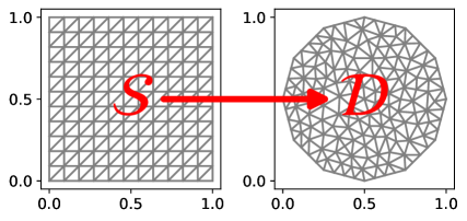
(a) Noise is sampled on $\mathcal{S}\supset\mathcal{D}$ and interpolated onto $\mathcal{D}$.

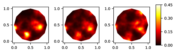
(b) A realization of $X_{h,\Delta t}$ at (left to right) $t_{j}=0.9,0.95$ and $1.0$.

Figure 1. Noise discretization idea as in Example 5.6 for multiplicative noise, with $\mathcal{D}$ a dodecagon.

We derive (3) under mild conditions on $q$, Assumption 3.4. To use the results of [23] for the SPDE approximation error bound, we construct $\tilde{W}$ as a standard cylindrical Wiener process on the RKHS $H_{q}(\mathcal{S})$ and derive new Hilbert–Schmidt bounds on multiplication operators and finite element interpolant products. Non-trivial techniques are needed for the noise discretization error, like entropy numbers of Sobolev space embeddings and generalized error bounds for interpolants. The analysis shows that the noise discretization error is non-dominant for most kernels in $d\geq 2$, (including the Matérn class), but dominant for some factorizable kernels in $d\geq 2$ and rough Matérn kernels in $d=1$. Moreover, there are settings where $r_{2}>1+r_{1}$, so that we may take $N_{h^{\prime}}\ll N_{h}$, increasing computational savings with retained accuracy.

Interpolation of noise in finite element approximations of (1) with $\mathcal{S}=\mathcal{D}$ was considered in [7], but without analyzing how the strong error is affected. Lemma 6.1 in [23] contains the only such analysis we are aware of. The author considers modified interpolants and spatial semidiscretization only, for $F=0,G=I,\mathcal{D}=(0,1),A=-\Delta$ with Dirichlet boundary conditions and $q$ given by a sine expansion. Then the convergence of the strong error is unaffected, but the author notes that

it is only barely analyzed in the literature, how [the replacement of $\Delta W^{j}$ with $I_{h}\Delta W^{j}$] affects the order of convergence. …We leave a rigorous justification in a more general situation as a subject to future research. [23, p. 139]

We give this justification in Section 4 and demonstrate it by numerical simulations in Section 5 for concrete example kernels. Sections 2-3 contain prerequisite material.

2. Notation and mathematical background

This paper employs generic constants $C$. These vary between occurrences and are independent of discretization parameters. We write $a\lesssim b$ for $a,b\in\amsmathbb{R}$ to signify $a\leq Cb$ for such a constant $C$.

2.1. Operator theory

For Banach spaces $U$ and $V$ (all over $\amsmathbb{R}$ unless otherwise stated), we denote by $\mathcal{L}(U,V)$ the linear and bounded operators from $U$ to $V$ and set $\mathcal{L}(U):=\mathcal{L}(U,U)$. We write $U\hookrightarrow V$ if $U\subset V$ and $\|I_{U\hookrightarrow V}\|_{\mathcal{L}}:=\|I_{U\hookrightarrow V}\|_{\mathcal{L}(U,V)}<\infty$.

For separable Hilbert spaces $U$ and $H$, $\mathcal{L}_{2}(U,H)$ is the space of Hilbert–Schmidt operators. It is an operator ideal and a separable Hilbert space with inner product

$$\langle\Gamma_{1},\Gamma_{2}\rangle_{\mathcal{L}_{2}(U,H)}:=\sum_{j=1}^{\infty}\langle\Gamma_{1}e_{j},\Gamma_{2}e_{j}\rangle_{H},\quad\Gamma_{1},\Gamma_{2}\in\mathcal{L}_{2}(U,H),$$

where $(e_{j})_{j=1}^{\infty}$ is an arbitrary orthonormal basis (ONB) of $U$. For $\Gamma\in\mathcal{L}(U,H)$, the range $\Gamma(U)$ is a Hilbert space with $\langle\cdot,\cdot\rangle_{\Gamma(U)}:=\langle\Gamma^{-1}\cdot,\Gamma^{-1}\cdot\rangle_{U}$, where $\Gamma^{-1}=(\Gamma|_{\ker(\Gamma)^{\perp}})^{-1}\colon\Gamma(U)\to\ker(\Gamma)^{\perp}\subset U$ is the pseudoinverse and $\ker(\Gamma)^{\perp}$ the orthogonal complement of the kernel of $\Gamma$. The norm on $\Gamma(U)$ is given by $\|u\|_{\Gamma(U)}:=\min_{v\in U,\Gamma v=u}\|v\|_{U}$. Note that $\Gamma^{-1}\Gamma$ coincides with the orthogonal projection $P_{\ker(\Gamma)^{\perp}}$, whereas $\Gamma\Gamma^{-1}=I$. We write $\Sigma^{+}(H)\subset\mathcal{L}(H)$ for the subspace of positive semidefinite operators on $H$ and refer to [29, Appendix C] for more details on these concepts.

2.2. Reproducing kernel Hilbert spaces

Let $q\colon\mathcal{D}\times\mathcal{D}\to\amsmathbb{R}$ be a positive semidefinite kernel on a non-empty connected subset $\mathcal{D}\subset\amsmathbb{R}^{d}$, $d\in\amsmathbb{N}$. The RKHS $H_{q}(\mathcal{D})$ of $q$ on $\mathcal{D}$ is the Hilbert space of functions on $\mathcal{D}$ such that

1. $q(x,\cdot)\in H_{q}(\mathcal{D})$ for all $x\in\mathcal{D}$ and

2. for all $f\in H_{q}(\mathcal{D}),x\in\mathcal{D}$, $f(x)=\langle f,q(x,\cdot)\rangle_{H_{q}(\mathcal{D})}$ (the reproducing property).

Each $q$ has a unique RKHS $(H_{q}(\mathcal{D}),\langle\cdot,\cdot\rangle_{H_{q}(\mathcal{D})})$, but $H_{q}(\mathcal{D})$ may have multiple equivalent norms for different kernels. A Hilbert space $H$ of functions on $\mathcal{D}$ is an RKHS if and only if the evaluation functional $\delta_{x}\colon H\to\amsmathbb{R}$, $\delta_{x}f:=f(x)$, is bounded for all $x\in\mathcal{D}$ [33, Theorem 10.2]. We write $H_{q}:=H_{q}(\mathcal{D})$ if $\mathcal{D}$ need not be emphasized. If $q$ is positive semidefinite on $\mathcal{S}\supset\mathcal{D}$, then the restriction $R_{\mathcal{S}\to\mathcal{D}}f$ of $f\in H_{q}(\mathcal{S})$ to a function on $\mathcal{D}$ belongs to $H_{q}(\mathcal{D})$ and $H_{q}(\mathcal{D})=R_{\mathcal{S}\to\mathcal{D}}(H_{q}(\mathcal{S}))$ with equal norms [6, Theorem 6]. Thus the pseudoinverse $R^{-1}_{\mathcal{S}\to\mathcal{D}}$ is an extension operator with $\|R^{-1}_{\mathcal{S}\to\mathcal{D}}\|_{\mathcal{L}(H_{q}(\mathcal{D}),H_{q}(\mathcal{S}))}=1$.

For continuous and bounded $q$, $H_{q}$ is separable [6, Corollary 4]. This yields

(5) $$q(x,\cdot)=\sum^{\infty}_{j=1}e_{j}(x)e_{j}(\cdot),\quad q(x,y)=\sum^{\infty}_{j=1}e_{j}(x)e_{j}(y),\quad x,y\in\mathcal{D},$$

for any ONB $(e_{j})_{j=1}^{\infty}$ with convergence in $H_{q}$ respectively $\amsmathbb{R}$. When $\mathcal{D}=\amsmathbb{R}^{d}$ and $q$ is of the form $q(x,y)=q(x-y)$, it is called stationary. If it also is continuous, bounded and integrable, it has a positive and integrable Fourier transform $\hat{q}\colon\amsmathbb{R}^{d}\to\amsmathbb{R}^{+}$ (the spectral density) [33, Chapter 6]. We refer to [6, 33] for more details on RKHSs.

2.3. Fractional Sobolev spaces

Let $\mathcal{D}\subset\amsmathbb{R}^{d}$, $d=1,2,3$ be a bounded Lipschitz domain. We let $H:=L^{2}(\mathcal{D})$ with inner product $\langle\cdot,\cdot\rangle$ and norm $\|\cdot\|$. We let $W^{r,p}(\mathcal{D})$, $r\in[0,\infty),p\in(1,\infty),$ denote the Sobolev space equipped with the norm

(6) $$\|u\|_{W^{r,p}(\mathcal{D})}:=\Big{(}\|u\|_{W^{m,p}(\mathcal{D})}^{p}+\sum_{|\alpha|=m}\int_{\mathcal{D}\times\mathcal{D}}\frac{|D^{\alpha}u(x)-D^{\alpha}u(y)|^{p}}{|x-y|^{d+p\sigma}}\,\mathrm{d}x\,\mathrm{d}y\Big{)}^{1/p},$$

for non-integer $r=m+\sigma$, $m\in\amsmathbb{N}_{0},\sigma\in(0,1)$, where $\|\cdot\|_{W^{m,p}(\mathcal{D})}$ is the integer order Sobolev norm and $|\cdot|$ the Euclidean norm on $\amsmathbb{R}^{d}$, see also [18, Definition 1.3.2.1]. The space $H^{r}(\mathcal{D}):=W^{r,2}(\mathcal{D})$ is a Hilbert space. We write $H^{r}:=H^{r}(\mathcal{D})$ and $W^{r,p}:=W^{r,p}(\mathcal{D})$ when $\mathcal{D}$ is not emphasized. The properties here and below, typically given for Sobolev spaces over $\amsmathbb{C}$, readily transfer to our setting in $\amsmathbb{R}$, cf. [22, Section 2.2].

For $r>d/2$, $\delta_{x}$ is bounded by the Sobolev embedding theorem, making $H^{r}$ an RKHS [18, Theorem 1.4.4.1]. The stationary kernel $q_{r}$ of the Bessel potential space $H^{r}(\amsmathbb{R}^{d})$ is given by the continuous and bounded function $q_{r}(x,y):=q_{r}(|x-y|):=2^{1-r}|x-y|^{r-d/2}K_{r-d/2}(|x-y|)/\Gamma(s)$ for $x,y\in\amsmathbb{R}^{d}$, where $K$ is the modified Bessel function of the second kind [33, p. 133]. Since $\mathcal{D}$ is Lipschitz, $H^{r}(\mathcal{D})=H_{q_{r}}(\mathcal{D})$ with equivalent norms, see [18, p. 25] and [33, Corollary 10.48]. The expressions (17) and (18) in [31, Section 2.7] yield for all $r\in(d/2,d/2+1)$,

(7) $$q_{r}(x,x)-2q_{r}(x,y)+q_{r}(y,y)=2(q_{r}(0)-q_{r}(|x-y|))\leq C|x-y|^{2r-d},\quad x,y\in\bar{\mathcal{D}},$$

for some constant $C<\infty$. When $r=d/2+1$, the exponent is replaced by $2r-d-\epsilon$ for arbitrary $\epsilon>0$. When $r>d/2+1$, it is replaced by $2$.

2.4. Fractional powers of elliptic operators

From here on, we let $\mathcal{D}$ be convex and define $A$ as the part in $H$ of the operator $A\colon V\mapsto V^{*}$ defined by ${}_{V^{*}}\langle Au,v\rangle_{V}:=a(u,v)$ for a Gelfand triple $V\hookrightarrow H\hookrightarrow V^{*}$ and bilinear form $a\colon V\times V\to\amsmathbb{R}$. We consider either Neumann-type homogeneous zero boundary conditions ($V:=H^{1}$) or Dirichlet-type ($V:=H^{1}_{0}(\mathcal{D})=\{v\in H^{1}:\mathrm{tr}(v)=0\}$ with $\mathrm{tr}$ the trace operator), with

$$a(u,v):=\sum_{i,j=1}^{d}\int_{\mathcal{D}}a_{i,j}D^{i}uD^{j}v\,\mathrm{d}x+\int_{\mathcal{D}}cuv\,\mathrm{d}x,\,u,v\in V.$$

The derivative $D^{j}$ is with respect to $x_{j}$, $a_{i,j}\in\mathcal{C}^{1}(\bar{\mathcal{D}})$ fulfill $a_{i,j}=a_{j,i}$ and for some $\lambda_{0}>0$ and all $y\in\amsmathbb{R}^{d},x\in\mathcal{D}$, $\sum^{d}_{i,j=1}a_{i,j}(x)y_{i}y_{j}\geq\lambda_{0}|y|^{2}$. The function $c\in L^{\infty}(\mathcal{D})$ is non-negative a.e. on $\mathcal{D}$. Without loss of generality, let $c\geq c_{0}$ for some $c_{0}>0$, a.e. on $\mathcal{D}$, in the Neumann case. Then $a$ is continuous, symmetric and coercive, and $A$ densely defined, closed and positive definite.

Since $V\hookrightarrow H$ is compact, $A$ has a compact inverse, enabling fractional powers by spectral decomposition. We write $\dot{H}^{r}:=\mathrm{dom}(A^{r/2})$ for $r\geq 0$ and let, for $r<0$, $\dot{H}^{r}$ be the completion of $H$ under $\|A^{r/2}\cdot\|$. Since $\mathcal{D}$ is convex, the functions of $\dot{H}^{2}$ are the elements of $H^{2}$ that satisfy the boundary conditions of $A$ while

(8) $$\dot{H}^{r}=H^{r},\,r\in[0,\theta)\text{ with }\theta:=\begin{cases}1/2&\text{ for Dirichlet boundary conditions and}\\ 3/2&\text{ for Neumann boundary conditions,}\end{cases}$$

with norm equivalence [34, Theorems 16.9, 16.13]. Moreover, $\dot{H}^{r}\hookrightarrow H^{r},r\in[0,2],$ by complex interpolation [3, Theorem 3.2, Remark 3.3]. We refer to [23, Appendix B] and [34, Chapter 2] for more on this setting.

3. Parabolic SPDEs driven by cylindrical Wiener processes in RKHSs

Here, mild solutions to (1) and cylindrical Wiener processes $W$ in $H_{q}(\mathcal{D})$ are introduced. We extend $W$ to $\mathcal{S}$, state our assumptions on $q$ and derive regularity in the setting of stochastic reaction-diffusion-advection equations.

3.1. Mild solutions of SPDEs

For $T<\infty$, let $(\Omega,\mathcal{F},(\mathcal{F}_{t})_{t\in[0,T]},\amsmathbb{P})$ be a filtered probability space under the usual conditions. The process on $[0,T]$ given by

(9) $$X(t):={S}(t)X(0)+\int_{0}^{t}{S}(t-s)F(X(s))\,\mathrm{d}s+\int_{0}^{t}{S}(t-s)G(X(s))\,\mathrm{d}W(s),$$

is called mild if also $X\in\mathcal{C}([0,T],L^{p}(\Omega,H))$, $p\geq 2$, where $S=(S(t))_{t\geq 0}$ is the analytic semigroup generated by $-A$. The stochastic integral is of Itô type [11, Chapter 4] and $W$ a standard cylindrical Wiener process in $H_{q}(\mathcal{D})$. In [23], the existence of a unique solution (9) is derived with the regularity estimate $\sup_{t\in[0,T]}\|X(t)\|_{L^{p}(\Omega,\dot{H}^{r+1})}<\infty.$ This is shown in [23, Theorem 2.27] under the following assumption.

Assumption 3.1.

For some $r\in[0,1)$, $p\geq 2$, there is a $C<\infty$ such that:

1. The initial value $X_{0}$ is $\mathcal{F}_{0}$-measurable and $\|X_{0}\|_{L^{p}(\Omega,\dot{H}^{r+1})}\leq C$.

2. The non-linear reaction-advection term $F\colon H\to\dot{H}^{r-1}$ satisfies

   1. $\|F(u)-F(v)\|_{\dot{H}^{-1}}\leq C\|u-v\|_{H}$ for all $u,v\in H$

   2. $\|F(u)-F(v)\|_{\dot{H}^{r-1}}\leq C\|u-v\|_{\dot{H}^{r}}$ for all $u,v\in\dot{H}^{r}$.

3. The non-linear multiplicative noise operator $G\colon H_{q}\to\dot{H}^{r}$ satisfies

   1. $\|G(u)\|_{\mathcal{L}_{2}(H_{q},\dot{H}^{r})}\leq C(1+\|u\|_{\dot{H}^{r}})$ for all $u\in\dot{H}^{r}$ and

   2. $\|G(u)-G(v)\|_{\mathcal{L}_{2}(H_{q},H)}\leq C\|u-v\|$ for all $u,v\in H$.

Assumption 3.1(a) depends on Sobolev regularity of $X_{0}$ and whether it satisfies the boundary conditions associated with $A$. Assumption 3.1(b) is with

(10) $$F(u):=F_{1}(u)+F_{2}(u):=b(\cdot)\cdot\nabla u+f(u(\cdot),\cdot)$$

satisfied for regular $b=(b_{1},\ldots,b_{d})\colon\mathcal{D}\to\amsmathbb{R}^{d}$, $f\colon\amsmathbb{R}\times\mathcal{D}\to\amsmathbb{R}$ and functions $u$ on $\mathcal{D}$. The next proposition gives sufficient conditions on $f$ and $b$ for this to hold true.

Proposition 3.2.

Let $F$ be given by (10), where for some constant $C<\infty$,

1. $\int_{\mathcal{D}}|f(0,x)|^{2}\,\mathrm{d}x\leq C$

2. $\operatorname*{ess\,sup}_{y\in\mathcal{D}}|f(x_{1},y)-f(x_{2},y)|\leq C|x_{1}-x_{2}|$, $x_{1},x_{2}\in\amsmathbb{R}$, and

3. $\operatorname*{ess\,sup}_{x\in\mathcal{D}}\sum_{j=1}^{2}\left(|b_{j}(x)|+\left|\frac{\partial b_{j}}{\partial x_{j}}(x)\right|\right)\leq C$.

Then $F$ extends to an operator on $H$ and fulfills Assumption 3.1(b) for all $r\in[0,1]$

1. under Dirichlet boundary conditions on $A$ and

2. under Neumann boundary conditions if also $b(x)=0$ for a.e. $x\in\partial\mathcal{D}$.

This result is derived for $F=F_{2}$ in [19, p. 120], recalling that $\dot{H}^{r}\hookrightarrow H$ for $r\geq 0$. The term $F_{1}$ is treated in [23, Example 2.22] in the Dirichlet case. The Neumann case follows analogously to this from Green’s formula, since $b$ vanishes on $\partial\mathcal{D}$.

For which $r$ Assumption 3.1(c) is satisfied when $G$ is a multiplication operator

(11) $$(G(u)v)(x):=g(u(x),x)v(x),\quad u\in H,v\in H_{q},x\in\mathcal{D},$$

depends largely on the covariance kernel $q$. In the next section, we specify our assumptions on $q$ and formally introduce the mathematical model of the noise $W$.

3.2. Cylindrical Wiener processes in RKHSs

A family, indexed by $t\in[0,T]$, of linear maps from a Hilbert space $U$ to the space of real-valued random variables is called a cylindrical stochastic process in $U$. Such a process $W$ is a (strongly) cylindrical Wiener process with covariance operator $Q\in\Sigma^{+}(U)$ if $t\mapsto(W(t)u_{1},\ldots,W(t)u_{n})$ is a Wiener process in $\amsmathbb{R}^{n}$ for $u_{1},\ldots,u_{n}\in U,n\in\amsmathbb{N},$ and $\operatorname{\amsmathbb{E}}[(W(t)u)(W(t)v)]=t\langle Qu,v\rangle_{U}$ for all $t\in[0,T],u,v\in U$. It is called standard if $Q=I$. For such $W$ in $U$, another Hilbert space $\tilde{U}$ and $\Gamma\in\mathcal{L}(U,\tilde{U})$ the process $\Gamma W$ defined by $t\mapsto W(t)(\Gamma^{*}v)$, $v\in\tilde{U}$, is a cylindrical Wiener process in $\tilde{U}$ with covariance $\Gamma Q\Gamma^{*}\in\Sigma^{+}(\tilde{U})$. Here $\Gamma^{*}\in\mathcal{L}(\tilde{U},U)$ is the adjoint of $\Gamma$. We have here followed the setting of [30] and [11, Section 4.1.2], identifying Hilbert spaces with their duals.

We now specify $W$ to be a standard cylindrical Wiener process in $H_{q}(\mathcal{D})$. With $W(t,x):=\delta_{x}W(t)$, one obtains by the reproducing property of $H_{q}$ a Gaussian random field with covariance $\operatorname{\amsmathbb{E}}[W(t,x)W(s,y)]=\min(t,s)q(x,y),s,t\in[0,T],x,y\in\mathcal{D}$. This yields that the interpolation (4), used for simulation of $W$ by sampling on $\mathcal{S}\supseteq\mathcal{D}$, is well-defined. However, we also need to confirm that an extension $\tilde{W}$ of $W$ to a standard cylindrical Wiener process in $H_{q}(\mathcal{S})$ exists, with $W=R_{\mathcal{S}\to\mathcal{D}}\tilde{W}$.

Lemma 3.3.

If $q$ is positive semidefinite on $\mathcal{S}$ there is a standard cylindrical Wiener process $\tilde{W}$ on $H_{q}(\mathcal{S})$ such that $R_{\mathcal{S}\to\mathcal{D}}\tilde{W}=W$.

Proof.

Recall that $\ker(R_{\mathcal{S}\to\mathcal{D}})$ is a Hilbert subspace of $H_{q}(\mathcal{S})=\ker(R_{\mathcal{S}\to\mathcal{D}})\oplus\ker(R_{\mathcal{S}\to\mathcal{D}})^{\perp}$. Let $\hat{W}$ be a cylindrical Wiener process on $H_{q}(\mathcal{S})$, independent of $W$, with covariance operator $P_{\ker(R_{\mathcal{S}\to\mathcal{D}})}$. Set $\tilde{W}:=R_{\mathcal{S}\to\mathcal{D}}^{-1}W+\hat{W}$. By independence, $t\mapsto(\tilde{W}(t)u_{1},\ldots,\tilde{W}(t)u_{n})$ is an $\amsmathbb{R}^{n}$-valued Wiener process for all $u_{1},\ldots,u_{n}\in H_{q}(\mathcal{S}),n\in\amsmathbb{N}$ and for all $u,v\in H_{q}(\mathcal{S})$, $\operatorname{\amsmathbb{E}}[(\tilde{W}(t)u)(\tilde{W}(t)v)]$ is given by

(12) $$\begin{split}&\operatorname{\amsmathbb{E}}[(W(t)(R_{\mathcal{S}\to\mathcal{D}}^{-1})^{*}u)(W(t)(R_{\mathcal{S}\to\mathcal{D}}^{-1})^{*}v)]+\operatorname{\amsmathbb{E}}[(\hat{W}(t)u)(\hat{W}(t)v)]\\ &\quad=t\langle R_{\mathcal{S}\to\mathcal{D}}^{-1}(R_{\mathcal{S}\to\mathcal{D}}^{-1})^{*}u,v\rangle_{H_{q}(\mathcal{S})}+t\langle P_{\ker(R_{\mathcal{S}\to\mathcal{D}})}u,v\rangle_{H_{q}(\mathcal{S})}.\end{split}$$

Since $v\in\ker(R_{\mathcal{S}\to\mathcal{D}})^{\perp}$ yields $v=R_{\mathcal{S}\to\mathcal{D}}^{-1}R_{\mathcal{S}\to\mathcal{D}}v$, and since $H_{q}(\mathcal{D})=R_{\mathcal{S}\to\mathcal{D}}(H_{q}(\mathcal{S}))$,

(13) $$\begin{split}\langle R_{\mathcal{S}\to\mathcal{D}}^{-1}(R_{\mathcal{S}\to\mathcal{D}}^{-1})^{*}u,v\rangle_{H_{q}(\mathcal{S})}&=\langle R_{\mathcal{S}\to\mathcal{D}}^{-1}(R_{\mathcal{S}\to\mathcal{D}}^{-1})^{*}u,R_{\mathcal{S}\to\mathcal{D}}^{-1}R_{\mathcal{S}\to\mathcal{D}}v\rangle_{H_{q}(\mathcal{S})}\\ &=\langle(R_{\mathcal{S}\to\mathcal{D}}^{-1})^{*}u,R_{\mathcal{S}\to\mathcal{D}}v\rangle_{H_{q}(\mathcal{D})}\\ &=\langle u,P_{\ker(R_{\mathcal{S}\to\mathcal{D}})^{\perp}}v\rangle_{H_{q}(\mathcal{S})},\quad v\in\ker(R_{\mathcal{S}\to\mathcal{D}})^{\perp}.\end{split}$$

Note now that for $x\in\mathcal{D}$ and $v\in H_{q}(\mathcal{S})$, $q(x,\cdot)=P_{\ker(R_{\mathcal{S}\to\mathcal{D}})^{\perp}}q(x,\cdot)$ as a result of

$$\langle(I-P_{\ker(R_{\mathcal{S}\to\mathcal{D}})^{\perp}})q(x,\cdot),v\rangle_{H_{q}(\mathcal{S})}=\langle q(x,\cdot),P_{\ker(R_{\mathcal{S}\to\mathcal{D}})}v\rangle_{H_{q}(\mathcal{S})}=(P_{\ker(R_{\mathcal{S}\to\mathcal{D}})}v)(x).$$

Since also $P_{\ker(R_{\mathcal{S}\to\mathcal{D}})^{\perp}}=R_{\mathcal{S}\to\mathcal{D}}^{-1}R_{\mathcal{S}\to\mathcal{D}}$ we find that $q(x,\cdot)=R_{\mathcal{S}\to\mathcal{D}}^{-1}q(x,\cdot)|_{\mathcal{D}}$ for $x\in\mathcal{D}$. Combining this with the reproducing property, we find that for $x\in\mathcal{D}$, $v\in\ker(R_{\mathcal{S}\to\mathcal{D}})$, $\langle R_{\mathcal{S}\to\mathcal{D}}^{-1}q(x,\cdot)|_{\mathcal{D}},v\rangle_{H_{q}(\mathcal{S})}=\langle q(x,\cdot),v\rangle_{H_{q}(\mathcal{S})}$. By approximating $(R_{\mathcal{S}\to\mathcal{D}}^{-1})^{*}u$ with linear combinations of $(q(x,\cdot))_{x\in\mathcal{D}}$ in $H_{q}(\mathcal{D})$ (see [6, Theorem 3]), we then obtain

(14) $$\langle R_{\mathcal{S}\to\mathcal{D}}^{-1}(R_{\mathcal{S}\to\mathcal{D}}^{-1})^{*}u,v\rangle_{H_{q}(\mathcal{S})}=0=\langle u,P_{\ker(R_{\mathcal{S}\to\mathcal{D}})^{\perp}}v\rangle_{H_{q}(\mathcal{S})},\quad v\in\ker(R_{\mathcal{S}\to\mathcal{D}}).$$

Combining (13) and (14) in (12) with the identity $P_{\ker(R_{\mathcal{S}\to\mathcal{D}})^{\perp}}+P_{\ker(R_{\mathcal{S}\to\mathcal{D}})}=I$ yields $\operatorname{\amsmathbb{E}}[(\tilde{W}(t)u)(\tilde{W}(t)v)]=t\langle u,v\rangle_{H_{q}(\mathcal{S})}$ which shows that $\tilde{W}$ is a standard cylindrical Wiener process on $H_{q}(\mathcal{S})$. The fact that $R_{\mathcal{S}\to\mathcal{D}}\tilde{W}=W$ now follows from the identities $R_{\mathcal{S}\to\mathcal{D}}P_{\ker(R_{\mathcal{S}\to\mathcal{D}})}=0$ and $R_{\mathcal{S}\to\mathcal{D}}R^{-1}_{\mathcal{S}\to\mathcal{D}}=I$ on $R_{\mathcal{S}\to\mathcal{D}}(H_{q}(\mathcal{S}))=H_{q}(\mathcal{D})$. ∎

We now state our main assumption for $q$ on $\mathcal{S}\supseteq\mathcal{D}$. Note that if $q$ satisfies this on $\mathcal{S}$, the corresponding assumption is also fulfilled for $\mathcal{D}$. The first part is used to verify Assumption 3.1(c), the second for the numerical analysis of Section 4.

Assumption 3.4.

The positive semidefinite kernel $q$ is bounded on $\mathcal{S}$ and satisfies

1. for some $\gamma\in(0,1]$ and $C<\infty$ the Hölder-type regularity condition

   $$q(x,x)-2q(x,y)+q(y,y)\leq C|x-y|^{2\gamma},\quad x,y\in\mathcal{S},$$

2. and for some $\mu>0$ and $\psi>d/\mu$ the embedding property $H_{q}(\mathcal{S})\hookrightarrow W^{\mu,\psi}(\mathcal{S})$.

Remark 3.5.

Since $q$ is bounded, $H_{q}(\mathcal{D})\hookrightarrow H=L^{2}(\mathcal{D})$. The embedding is Hilbert–Schmidt, since continuity of $q$ yields an ONB $(e_{j})_{j=1}^{\infty}$ of $H_{q}$ such that

$$\|I_{H_{q}\hookrightarrow H}\|_{\mathcal{L}_{2}}^{2}:=\|I_{H_{q}\hookrightarrow H}\|_{\mathcal{L}_{2}(H_{q},H)}^{2}=\sum_{j=1}^{\infty}\int_{\mathcal{D}}e_{j}(x)^{2}\,\mathrm{d}x=\int_{\mathcal{D}}q(x,x)\,\mathrm{d}x<\infty,$$

see (5). Therefore, $W$, viewed as cylindrical in $H$, is under Assumption 3.4 induced by a so called $Q$-Wiener process with covariance $Q:=I_{H_{q}\hookrightarrow H}I^{*}_{H_{q}\hookrightarrow H}\in\Sigma^{+}(H)$ [30, Theorem 8.1]. The relation to the original process is given by $W(t)(I^{*}_{H_{q}\hookrightarrow H}u)=\langle W_{Q}(t),u\rangle$ for $u\in H$. The operator $Q$ is of integral type with kernel $q$. We could equivalently work with $W_{Q}$ instead of $W$ in (1), but the frequent use of the RKHS properties in Section 2.2 would make the notation and analysis cumbersome.

3.3. Non-linear multiplicative noise operator

We prove a result relating the Hölder-type regularity of $q$ in Assumption 3.4(a) to Assumption 3.1(c) on $G$ when $g\colon\amsmathbb{R}\times\mathcal{D}\to\amsmathbb{R}$ in (11) satisfies, for some constant $C<\infty$,

(15) $$|g(x_{1},y_{1})-g(x_{2},y_{2})|\leq C(|x_{1}-x_{2}|+|y_{1}-y_{2}|),\quad x_{1},x_{2}\in\amsmathbb{R},y_{1},y_{2}\in\mathcal{D}.$$

In the special case where $q$ has a known expansion (Example 5.5 below), $A$ has Dirichlet boundary conditions and $\mathcal{D}=[0,1]^{d},d\in\amsmathbb{N}$, it was derived in [19, Section 4]. We extend this setting to more general kernels, domains and boundary conditions.

Proposition 3.6.

Let $G$ be given by (11) where $g$ satisfies (15). Under Assumption 3.4(a), there is for all $r\in[0,\gamma)$ a constant $C<\infty$ such that

1. $\|G(u)-G(v)\|_{\mathcal{L}_{2}(H_{q}(\mathcal{D}),H)}\leq C\|u-v\|$ for all $u,v\in H$ and

2. $\|G(u)\|_{\mathcal{L}_{2}(H_{q}(\mathcal{D}),H^{r})}\leq C(1+\|u\|_{H^{r}})$ for all $u\in H^{r}$.

Therefore, Assumption 3.1(c) is satisfied for all $r<\min(\gamma,\theta)$, with $\theta$ as in (8).

Proof.

Note first that Assumption 3.4(a) along with the reproducing property of $H_{q}$ yields that all $v\in H_{q}$ are bounded. Moreover, (15) ensures that $\|g(u(\cdot),\cdot)\|^{2}\lesssim 1+\|u\|^{2}$ for $u\in H$ so that $G(u)(v)$ indeed takes values in $H$ for $v\in H_{q}$.

By Assumption 3.4(a), $H_{q}$ is separable with an ONB $(e_{j})_{j=1}^{\infty}$. By Tonelli’s theorem and the decomposition (5) for the bounded kernel $q$, $G$ maps into $\mathcal{L}_{2}(H_{q}(\mathcal{D}),H)$ since

$$\|G(u)\|_{\mathcal{L}_{2}(H_{q},H)}^{2} =\sum_{j=1}^{\infty}\int_{\mathcal{D}}g(u(x),x)^{2}e_{j}(x)^{2}\,\mathrm{d}x$$

$$\leq\left(\sup_{x\in\mathcal{D}}q(x,x)\right)\int_{\mathcal{D}}g(u(x),x)^{2}\,\mathrm{d}x\lesssim\int_{\mathcal{D}}x^{2}+|u(x)|^{2}\,\mathrm{d}x.$$

Similarly, the claim (i) is obtained from the Lipschitz regularity of $g$, as

$$\|G(u)-G(v)\|_{\mathcal{L}_{2}(H_{q},H)}^{2}\leq\left(\sup_{x\in\mathcal{D}}q(x,x)\right)\int_{\mathcal{D}}\left(g(u(x),x)-g(v(x),x)\right)^{2}q(x,x)\,\mathrm{d}x.$$

can be bounded by $C\|u(x)-v(x)\|^{2}$ for some $C<\infty$. To prove (ii), we note that the definition of $\|\cdot\|_{H^{r}}=\|\cdot\|_{W^{r,2}}$ yields that $\|G(u)\|_{\mathcal{L}_{2}(H_{q},H^{r})}^{2}$ is given by

$$\sum_{j=1}^{\infty}\int_{\mathcal{D}}|(G(u)e_{j})(x)|^{2}\,\mathrm{d}x+\sum_{j=1}^{\infty}\int_{\mathcal{D}\times\mathcal{D}}\frac{|(G(u)e_{j})(x)-(G(u)e_{j})(y)|^{2}}{|x-y|^{d+2r}}\,\mathrm{d}x\,\mathrm{d}y.$$

The first of these terms, $\|G(u)\|_{\mathcal{L}_{2}(H_{q},H)}^{2}$, was bounded above. For the second,

(16) $$\begin{split}&\sum_{j=1}^{\infty}\int_{\mathcal{D}\times\mathcal{D}}\frac{|(G(u)e_{j})(x)-(G(u)e_{j})(y)|^{2}}{|x-y|^{d+2r}}\,\mathrm{d}x\,\mathrm{d}y\\ &\quad=\int_{\mathcal{D}\times\mathcal{D}}\frac{\sum_{j=1}^{\infty}|g(u(x),x)e_{j}(x)-g(u(y),y)e_{j}(y)|^{2}}{|x-y|^{d+2r}}\,\mathrm{d}x\,\mathrm{d}y\\ &\quad\leq 2\int_{\mathcal{D}\times\mathcal{D}}\frac{\big{(}\sum_{j=1}^{\infty}(e_{j}(y))^{2}\big{)}|g(u(x),x)-g(u(y),y)|^{2}}{|x-y|^{d+2r}}\,\mathrm{d}x\,\mathrm{d}y\\ &\qquad+2\int_{\mathcal{D}\times\mathcal{D}}\frac{\big{(}\sum_{j=1}^{\infty}(e_{j}(x)-e_{j}(y))^{2}\big{)}|g(u(x),x)|^{2}}{|x-y|^{d+2r}}\,\mathrm{d}x\,\mathrm{d}y.\end{split}$$

In the first integral, we use (5), (15) and Assumption 3.4(a) to see that

$$\int_{\mathcal{D}\times\mathcal{D}}q(y,y)\frac{|g(u(x),x)-g(u(y),y)|^{2}}{|x-y|^{d+2r}}\,\mathrm{d}x\,\mathrm{d}y$$

$$\quad\leq\left(\sup_{x\in\mathcal{D}}q(x,x)\right)\int_{\mathcal{D}\times\mathcal{D}}\frac{|g(u(x),x)-g(u(y),y)|^{2}}{|x-y|^{d+2r}}\,\mathrm{d}x\,\mathrm{d}y$$

$$\quad\lesssim\int_{\mathcal{D}\times\mathcal{D}}\frac{|u(x)-u(y)|^{2}}{|x-y|^{d+2r}}\,\mathrm{d}x\,\mathrm{d}y+\int_{\mathcal{D}\times\mathcal{D}}|x-y|^{-2r}\,\mathrm{d}x\,\mathrm{d}y\lesssim\|u\|_{H^{r}}^{2}+1,$$

since $r<\gamma\leq 1$. The second integral in (LABEL:eq:prop:G-reg:2) is bounded by

$$\int_{\mathcal{D}\times\mathcal{D}}\frac{g(u(x),x)^{2}\big{(}q(x,x)-2q(x,y)+q(y,y)\big{)}}{|x-y|^{d+2r}}\,\mathrm{d}x\,\mathrm{d}y$$

$$\quad\leq\Big{(}\sup_{x\neq y\in\mathcal{D}}\frac{q(x,x)-2q(x,y)+q(y,y)}{|x-y|^{2\gamma}}\Big{)}$$

$$\hskip 30.00005pt\times\left(\sup_{x\in\mathcal{D}}\int_{\mathcal{D}}|x-y|^{2(\gamma-r)-d}\,\mathrm{d}y\right)\int_{\mathcal{D}}|g(u(x),x)|^{2}\,\mathrm{d}x\lesssim 1+\|u\|^{2}.$$

Assumption 3.1(c) follows directly from the fact that $\dot{H}^{r}=H^{r}$ for $r<\theta$ in (8). ∎

Since $\gamma\leq 1$, the bound by $\theta$ on $r$ in Proposition 3.6 only applies in the Dirichlet case. It can be dropped if $q(x,\cdot)=0$ or if $g(0,x)=0$ for all $x\in\partial\mathcal{D}$ [34, Theorem 16.13]. Moreover, the result is sharp. Too see this, consider Neumann boundary conditions and $H_{q}(\mathcal{D}):=H^{s}$ for $s\in(d/2,d/2+1)$, so that $\gamma=s-d/2$ in Assumption 3.4(a) by (7). If we let $g(x,y):=1$ for $x\in\amsmathbb{R},y\in\mathcal{D}$, we have $\|G(u)\|_{\mathcal{L}_{2}(H_{q},H^{r})}=\|I_{H^{s}\hookrightarrow H^{r}}\|_{\mathcal{L}_{2}}$ for $u\in H^{r}$. Proposition 3.6 shows that $\|I_{H^{s}\hookrightarrow H^{r}}\|_{\mathcal{L}_{2}}<\infty$ for $r<s-d/2$ whereas $\|I_{H^{s}\hookrightarrow H^{r}}\|_{\mathcal{L}_{2}}=\infty$ if $r=s-d/2$, see, e.g., [22, Lemma 2.3].

4. Piecewise linear interpolation of noise in SPDE approximations

By Lemma 3.3 we write without loss of regularity the mild solution $X$ of (9) as

$$X(t)={S}(t)X(0)+\int_{0}^{t}{S}(t-s)F(X(s))\,\mathrm{d}s+\int_{0}^{t}{S}(t-s)G(X(s))R_{\mathcal{S}\to\mathcal{D}}\,\mathrm{d}\tilde{W}(s),$$

for $t\in(0,T]$ and a standard cylindrical Wiener process $\tilde{W}$ on $H_{q}(\mathcal{S})$. We approximate $X$ by $X_{h,\Delta t}$ through the semi-implicit Euler scheme and piecewise linear finite elements. This was analyzed in [23], here we consider the additional noise discretization error coming from sampling $\tilde{W}$ pointwise on $\mathcal{S}$ and interpolating onto $\mathcal{D}$.

4.1. Discretization setting

From here on, we let $\mathcal{D}$ and $\mathcal{S}$ be polyhedral, as is common for finite element methods to avoid dealing with curved boundaries [8]. Consider two triangulations $\mathcal{T}_{h},\mathcal{T}_{h^{\prime}}$ on $\mathcal{D}$ and $\mathcal{S}$ with maximal mesh sizes $h,h^{\prime}\in(0,1]$, and let $V_{h}\subset H^{1}(\mathcal{D})$ and $V_{h^{\prime}}\subset H^{1}(\mathcal{S})$ be the spaces of piecewise linear functions on these. By $I_{h}$ and $I_{h^{\prime}}$ we denote the piecewise linear interpolants with respect to $\mathcal{T}_{h}$ and $\mathcal{T}_{h^{\prime}}$. For a function $v$ on $\mathcal{D}$, $v_{h}=:I_{h}v$ is the unique function $v_{h}\in V_{h}$ such that $v_{h}(x_{j})=v(x_{j})$ for all nodes $x_{j}$ of $\mathcal{T}_{h}$. In terms of the nodal basis functions $\varphi^{h}_{j}$,

$$I_{h}v=\Big{(}\sum_{j=1}^{N_{h}}\delta_{x_{j}}\varphi^{h}_{j}\Big{)}v=\sum_{j=1}^{N_{h}}v(x_{j})\varphi^{h}_{j},$$

where $N_{h}=\dim(V_{h})$ is the number of nodes. We need two results on these interpolants. The first generalizes the results in [4] to $p\neq 2$, with a proof in Appendix A.

Proposition 4.1.

Let $\mathcal{D}\subset\amsmathbb{R}^{d},d\leq 3$, be polyhedral with regular triangulation $\mathcal{T}_{h}$. Let $1<p<\infty$, $sp>d$ and $r\in[0,s]\cap[0,1+1/p)$. Assume also that $\mathcal{T}_{h}$ is quasiuniform for $s<1$ and $r>0$. Then, there is a $C<\infty$ such that

$$\|(I-I_{h})v\|_{W^{r}_{p}}\leq Ch^{\min(s-r,2)}\|v\|_{W^{s}_{p}}\text{ for all }h\in(0,1],v\in W^{s}_{p}(\mathcal{D}).$$

Lemma 4.2.

Let $\mathcal{D}\subset\mathcal{S}\subset\amsmathbb{R}^{d},d\leq 3,$ be polyhedral domains with triangulations $\mathcal{T}_{h}$ and $\mathcal{T}_{h^{\prime}}$. Let $q$ be a bounded and continuous positive semidefinite kernel on $\mathcal{S}$. Let $B\in\mathcal{L}(L^{\infty}(\mathcal{D}),L^{2}(\mathcal{D}))$ be given by $(Bv)(x):=b(x)v(x)$ for a.e. $x\in\mathcal{D}$. Then

$$\|BI_{h}R_{\mathcal{S}\to\mathcal{D}}I_{h^{\prime}}\|_{\mathcal{L}_{2}(H_{q}(\mathcal{S}),L^{2}(\mathcal{D}))}\leq 2\sup_{x,y\in\mathcal{S}}\sqrt{|q(x,y)|}\|b\|_{L^{2}(\mathcal{D})}\text{ for all }b\in L^{2}(\mathcal{D}).$$

Proof.

Let us write $\varphi^{h}$ and $\varphi^{h^{\prime}}$ for the nodal bases on $V_{h}$ and $V_{h^{\prime}}$. Then

$$\|BI_{h}R_{\mathcal{S}\to\mathcal{D}}I_{h^{\prime}}\|_{\mathcal{L}_{2}(H_{q}(\mathcal{S}),L^{2}(\mathcal{D}))}^{2}=\sum_{j=1}^{\infty}\int_{\mathcal{D}}\Big{|}b(x)\sum_{k=1}^{N_{h^{\prime}}}\sum_{\ell=1}^{N_{h}}\varphi^{h^{\prime}}_{k}(x_{\ell})\varphi^{h}_{\ell}(x)e_{j}(x_{k})\Big{|}^{2}\,\mathrm{d}x.$$

Using (5), this can be written as

$$\int_{\mathcal{D}}b(x)^{2}\sum_{k,m=1}^{N_{h^{\prime}}}\sum_{\ell,n=1}^{N_{h}}\varphi^{h^{\prime}}_{k}(x_{\ell})\varphi^{h^{\prime}}_{m}(x_{n})\varphi^{h}_{\ell}(x)\varphi^{h}_{\ell}(x)\varphi^{h}_{n}(x)q(x_{k},x_{m})\,\mathrm{d}x$$

$$\quad=\sum_{m=1}^{N_{h^{\prime}}}\sum_{n=1}^{N_{h}}\int_{\mathcal{D}}b(x)^{2}\left(I_{h}R_{\mathcal{S}\to\mathcal{D}}I_{h^{\prime}}q(\cdot,x_{m})\right)(x)\varphi^{h}_{n}(x)\varphi^{h^{\prime}}_{m}(x_{n})\,\mathrm{d}x.$$

By stability of $I_{h}$ and $I_{h^{\prime}}$ in $L^{\infty}$, $|I_{h}R_{\mathcal{S}\to\mathcal{D}}I_{h^{\prime}}q(\cdot,x_{m})|\leq\sup_{x,y\in\mathcal{S}}|q(x,y)|$. Moreover, $\varphi^{h},\varphi^{h^{\prime}}$ are non-negative, sum to $1$ and $\varphi^{h^{\prime}}_{m}(x_{n})\neq 0$ for at most $4$ indices $m$. Thus,

$$\|BI_{h}R_{\mathcal{S}\to\mathcal{D}}I_{h^{\prime}}\|_{\mathcal{L}_{2}(H_{q}(\mathcal{S}),L^{2}(\mathcal{D}))}^{2} \leq 4\sup_{x,y\in\mathcal{S}}|q(x,y)|\int_{\mathcal{D}}b(x)^{2}\sum_{n=1}^{N_{h}}\varphi^{h}_{n}(x)\,\mathrm{d}x$$

$$=4\sup_{x,y\in\mathcal{S}}|q(x,y)|\int_{\mathcal{D}}b(x)^{2}\,\mathrm{d}x$$

$$=4\sup_{x,y\in\mathcal{S}}|q(x,y)|\|b\|_{L^{2}(\mathcal{D})}^{2}.$$

∎

We next set $\dot{V}_{h}:=V_{h}\cap\dot{H}^{1}$ and denote by $\dot{P}_{h}\colon H\to\dot{V}_{h}$ and $\dot{R}_{h}\colon\dot{H}^{1}\to\dot{V}_{h}$ the orthogonal projections under the topologies of $H$ and $\dot{H}^{1}$, respectively. Let $A_{h}\in\Sigma^{+}(V_{h})$ be defined by $\langle A_{h}u_{h},v_{h}\rangle:=a(u_{h},v_{h})$ for $u_{h},v_{h}\in\dot{V}_{h}$ so that $\|A_{h}^{1/2}v_{h}\|=\|v_{h}\|_{\dot{H}^{1}}$. Combining this equality with [23, (3.15)], we find $C_{1},C_{2}\in(0,\infty)$ such that

(17) $$C_{1}\|v_{h}\|_{\dot{H}^{r}}\leq\|A_{h}^{\frac{r}{2}}v_{h}\|_{H}\leq C_{2}\|v_{h}\|_{\dot{H}^{r}},\quad v_{h}\in\dot{V}_{h},h\in(0,1],r\in[-1,1],$$

using also an interpolation argument. With this, we can introduce $X_{h,\Delta t}$. For a time step ${\Delta t}\in(0,1]$, let $(t_{j})_{j=0}^{\infty}$ be given by $t_{j}={\Delta t}j$ and $N_{\Delta t}+1=\inf\{j\in\amsmathbb{N}:t_{j}\notin[0,T]\}$. Set $X_{h,\Delta t}^{0}:=\dot{P}_{h}X_{0}$ and let $X_{h,\Delta t}^{j}$ solve

(18) $$X_{h,\Delta t}^{j}-X_{h,\Delta t}^{j-1}+\Delta t(A_{h}X_{h,\Delta t}^{j}+\dot{P}_{h}F(X_{h,\Delta t}^{j-1}))=\dot{P}_{h}G(X_{h,\Delta t}^{j-1})I_{h}R_{\mathcal{S}\to\mathcal{D}}I_{h^{\prime}}\Delta\tilde{W}^{j}$$

for $j=1,\ldots,N_{\Delta t}$. Here $\Delta\tilde{W}^{j}:=\tilde{W}(t_{j})-\tilde{W}(t_{j-1})$. This is the same approximation as that of [23, Section 3.6], but with $\Delta W^{j}:=R_{\mathcal{S}\to\mathcal{D}}\Delta\tilde{W}^{j}$ replaced by $I_{h}R_{\mathcal{S}\to\mathcal{D}}I_{h^{\prime}}\Delta\tilde{W}^{j}$.

Let us write $S_{h,{\Delta t}}:=(I+{\Delta t}A_{h})^{-1}\dot{P}_{h}$. As in [23, (3.38)], for some $C<\infty$,

(19) $$\|A_{h}^{\frac{r}{2}}S_{h,{\Delta t}}^{j}\|_{\mathcal{L}(H)}\leq Ct_{j}^{-r/2},\quad h\in(0,1],r\in[0,2],j=1,\ldots N_{\Delta t}+1.$$

For all $n=0,\ldots,N_{\Delta t}$, we can write $X^{n}_{h,\Delta t}$ in closed form as

$$X^{n}_{h,\Delta t}=S^{n}_{h,\Delta t}X_{0}+\Delta t\sum^{n-1}_{j=0}S^{n-j}_{h,\Delta t}F(X^{j}_{h,\Delta t})+\sum^{n-1}_{j=0}S^{n-j}_{h,\Delta t}G(X_{h,\Delta t}^{j})I_{h}R_{\mathcal{S}\to\mathcal{D}}I_{h^{\prime}}\Delta\tilde{W}^{j}.$$

4.2. The main result

In this section, we derive an error bound on $X-X_{h,\Delta t}$ under noise interpolation. First, we need a regularity estimate for $X_{h,\Delta t}$.

Lemma 4.3.

Suppose $X_{0}$ and $F$ satisfy Assumption 3.1(a)-(b) for some $p\geq 2,r\in[0,1)$. Suppose also that $q$ satisfies Assumption 3.4(a) and let $G$ in (11) satisfy (15). Then, there is for all $s\in[0,1)$ a constant $C<\infty$ such that

$$\sup_{n\in\{1,\ldots,N_{\Delta t}\}}\|X_{h,\Delta t}^{n}\|_{L^{p}(\Omega,\dot{H}^{s})}\leq C\text{ for all }\Delta t,h,h^{\prime}\in(0,1].$$

Proof.

By the Burkholder–Davis–Gundy (BDG) inequality [11, Theorem 4.36]:

(20) $$\begin{split}\|X_{h,\Delta t}^{n}\|_{L^{p}(\Omega,\dot{H}^{s})}^{2}&\lesssim\|S^{n}_{h,\Delta t}X_{0}\|_{L^{p}(\Omega,\dot{H}^{s})}^{2}+\Big{\|}\Delta t\sum^{n-1}_{j=0}S^{n-j}_{h,\Delta t}F(X^{j}_{h,\Delta t})\Big{\|}_{L^{p}(\Omega,\dot{H}^{s})}^{2}\\ &\quad+\Delta t\sum^{n-1}_{j=0}\|S^{n-j}_{h,\Delta t}G(X_{h,\Delta t}^{j})I_{h}R_{\mathcal{S}\to\mathcal{D}}I_{h^{\prime}}\|_{L^{p}(\Omega,\mathcal{L}_{2}(H_{q}(\mathcal{S}),\dot{H}^{s}))}^{2}.\end{split}$$

For the last of these terms, we use (17), (19), Lemma 4.2 and (15) to bound it by

$$\Delta t\sum^{n-1}_{j=0}\|A_{h}^{\frac{s}{2}}S^{n-j}_{h,\Delta t}G(X_{h,\Delta t}^{j})I_{h}R_{\mathcal{S}\to\mathcal{D}}I_{h^{\prime}}\|_{L^{p}(\Omega,\mathcal{L}_{2}(H_{q}(\mathcal{S}),H))}^{2}$$

$$\quad\lesssim\Delta t\sum^{n-1}_{j=0}t_{n-j}^{-s}\|G(X_{h,\Delta t}^{j})I_{h}R_{\mathcal{S}\to\mathcal{D}}I_{h^{\prime}}\|_{L^{p}(\Omega,\mathcal{L}_{2}(H_{q}(\mathcal{S}),H))}^{2}$$

$$\quad\lesssim\Delta t\sum^{n-1}_{j=0}t_{n-j}^{-s}\|g(X_{h,\Delta t}^{j})\|_{L^{p}(\Omega,H)}^{2}\lesssim\Delta t\sum^{n-1}_{j=0}t_{n-j}^{-s}(1+\|X_{h,\Delta t}^{j}\|_{L^{p}(\Omega,H)}^{2}).$$

The first two terms of (20) are similarly bounded using (17), (19) and Assumption 3.1(a)-(b). A discrete Gronwall lemma, [23, Lemma A.4], completes the proof. ∎

In our main result, we show that noise interpolation results in an additional error $(h^{\prime})^{r_{2}}$, with a rate that depends on Assumption 3.4 as well as the dimension $d$. We assume the triangulations $\mathcal{T}_{h}$ and $\mathcal{T}_{h^{\prime}}$ to be quasiuniform, but see Remark 4.5.

Theorem 4.4.

Let $q$ satisfy Assumption 3.4 for some $\gamma>0,\mu>0,\psi>d/\mu$ and

$$\mu_{d}:=\mu-\max(d/2-1,d/\psi-1,0).$$

Let $X_{0}$ and $F$ satisfy Assumption 3.1(a)-(b) for $p\geq 2,r=r_{1}\in[0,\min(\gamma,\theta))$ with $\theta$ as in (8), and let $G$ in (11) satisfy (15). Suppose $\mathcal{T}_{h}$ and $\mathcal{T}_{h^{\prime}}$ are quasiuniform and let $h\leq Ch^{\prime}$ with $C<\infty$. For all $r_{2}\in[0,2]\cap[0,\mu_{d})$, there is a $C<\infty$ such that

$$\sup_{n\in\{1,\ldots,N_{\Delta t}\}}\|X(t_{n})-X_{h,\Delta t}^{n}\|_{L^{p}(\Omega,H)}\leq C(h^{1+r_{1}}+\Delta t^{1/2}+(h^{\prime})^{r_{2}})\quad\Delta t,h,h^{\prime}\in(0,1].$$

Proof of Theorem 4.4.

Note, that if $\mu_{d}\leq 0$, which can only occur in $d=3$, the error is simply bounded by regularity of (9) and Lemma 4.3. Below, we let $\mu_{d}>0$.

If we make the split $X(t_{n})-X_{h,\Delta t}^{n}=(X(t_{n})-X_{h,\Delta t}^{n}+\mathrm{I}^{n})-\mathrm{I}^{n}$ for

$$\mathrm{I}^{n}:=\sum^{n-1}_{j=0}S^{n-j}_{h,\Delta t}G(X_{h,\Delta t}^{j})(R_{\mathcal{S}\to\mathcal{D}}-I_{h}R_{\mathcal{S}\to\mathcal{D}}I_{h^{\prime}})\Delta\tilde{W}^{j},$$

the error $X(t_{n})-X_{h,\Delta t}^{n}+\mathrm{I}^{n}$ is of the same form as the error without noise interpolation in [23, Theorem 3.14]. Since $\mathcal{D}$ is convex, elliptic regularity yields $\sup_{h\in(0,1]}h^{-r}\|I-\dot{R}_{h}\|_{\mathcal{L}(\dot{H}^{r},H)}\lesssim 1$ for $r\in\{1,2\}$ (see [15, p. 799]) so that [23, Assumption 3.3] is satisfied. Moreover, [23, Assumption 3.5] is satisfied by quasiuniformity, all assumptions of [23, Section 2.3] are satisfied by Assumption 3.1 (through Proposition 3.6) and $X_{h,\Delta t}^{n}$ is bounded by Lemma 4.3. Thus, it suffices to bound $\mathrm{I}^{n}$, since by [23, Theorem 3.14],

$$\sup_{n\in\{1,\ldots,N_{\Delta t}\}}\|X(t_{n})-X_{h,\Delta t}^{n}+\mathrm{I}^{n}\|_{L^{p}(\Omega,H)}\lesssim h^{1+r_{1}}+\Delta t^{1/2}.$$

For the bound on $\mathrm{I}^{n}$, we use entropy numbers $(\epsilon_{j}(\Gamma))_{j=1}^{\infty}$ for operators $\Gamma\in\mathcal{L}(U,V)$ on Banach spaces $U,V$, see [28, Definition 12.1.2]. If we write $\|\Gamma\|_{\mathcal{E}^{\infty}(U,V)}:=\|\Gamma\|_{\mathcal{L}(U,V)}$ and $\|\Gamma\|_{\mathcal{E}^{\rho}(U,V)}:=\|(\epsilon_{j}(\Gamma))_{j=1}^{\infty}\|_{\ell^{\rho}},\rho\in(1,\infty),$ then a Hölder-type property holds for a further Banach space $E$ and operator $\Lambda\in\mathcal{L}(V,E)$:

(21) $$\|\Lambda\Gamma\|_{\mathcal{E}^{\rho}(U,E)}\leq 2\|\Lambda\|_{\mathcal{E}^{\rho_{1}}(V,E)}\|\Gamma\|_{\mathcal{E}^{\rho_{2}}(U,V)},\quad\rho_{1},\rho_{2}\in(1,\infty],1/{\rho}=1/{\rho_{1}}+1/{\rho_{2}}.$$

This follows from Theorems 12.1.3-5 and 14.2.3 in [28]. By [14, Theorem 3.5] and an equivalence of Sobolev and Besov spaces (see [3, Section 2]), we have

(22) $$\|I_{W^{s,\rho_{1}}(\mathcal{U})\hookrightarrow W^{r,\rho_{2}}(\mathcal{U})}\|_{\mathcal{E}^{\rho}}:=\|I_{W^{s,\rho_{1}}(\mathcal{U})\hookrightarrow W^{r,\rho_{2}}(\mathcal{U})}\|_{\mathcal{E}^{\rho}(W^{s,\rho_{1}}(\mathcal{U}),W^{r,\rho_{2}}(\mathcal{U}))}<\infty$$

for Lipschitz domains $\mathcal{U}$, $s,r\in\amsmathbb{R}^{+}\setminus\amsmathbb{N}$, $s-r>\max(d/\rho_{1}-d/\rho_{2},0)$ and $\rho>d/(s-r)$.

For Hilbert spaces $U,V$ and $\Gamma\in\mathcal{L}(U,V)$, Theorems 11.3.4, 11.4.2, 12.3.1 and 15.5.5 in [28] yield that $\|\Gamma\|_{\mathcal{L}_{2}(U,V)}\lesssim\|\Gamma\|_{\mathcal{E}^{2}(U,V)}$. Using also the BDG inequality,

$$\|\mathrm{I}^{n}\|_{L^{p}(\Omega,H)}^{2}\lesssim\Delta t\sum^{n-1}_{j=0}\operatorname{\amsmathbb{E}}\Big{[}\|S^{n-j}_{h,\Delta t}G(X_{h,\Delta t}^{j})\big{(}R_{\mathcal{S}\to\mathcal{D}}-I_{h}R_{\mathcal{S}\to\mathcal{D}}I_{h^{\prime}}\big{)}\|_{\mathcal{E}^{2}(H_{q}(\mathcal{S}),H)}^{p}\Big{]}^{\frac{2}{p}}.$$

This splits into $\|\mathrm{I}^{n}\|_{L^{p}(\Omega,H)}^{2}\lesssim\|\mathrm{II}^{n}\|_{L^{p}(\Omega,H)}^{2}+\|\mathrm{III}^{n}\|_{L^{p}(\Omega,H)}^{2}+\|\mathrm{IV}^{n}\|_{L^{p}(\Omega,H)}^{2}$ by

$$R_{\mathcal{S}\to\mathcal{D}}-I_{h}R_{\mathcal{S}\to\mathcal{D}}I_{h^{\prime}}=R_{\mathcal{S}\to\mathcal{D}}(I-I_{h^{\prime}})+(I-I_{h})R_{\mathcal{S}\to\mathcal{D}}-(I-I_{h})R_{\mathcal{S}\to\mathcal{D}}(I-I_{h^{\prime}}).$$

The three terms are treated similarly. We only consider the most complex case,

$$\|\mathrm{IV}^{n}\|_{L^{p}(\Omega,H)}^{2}:=\Delta t\sum^{n-1}_{j=0}\operatorname{\amsmathbb{E}}\Big{[}\|S^{n-j}_{h,\Delta t}G(X_{h,\Delta t}^{j})\big{(}(I-I_{h})R_{\mathcal{S}\to\mathcal{D}}(I-I_{h^{\prime}})\big{)}\|_{\mathcal{E}^{2}(H_{q}(\mathcal{S}),H)}^{p}\Big{]}^{\frac{2}{p}}.$$

We start by assuming $d>1$, and derive three preliminary bounds.

First, commutativity of $S^{n-j}_{h,\Delta t}$ and $A_{h}$, (21), (17) and (22) yield

$$\Delta t\sum^{n-1}_{j=0}\|S^{n-j}_{h,\Delta t}\|_{\mathcal{E}^{\alpha}(H,H)}^{2} =\Delta t\sum^{n-1}_{j=0}\|A_{h}^{\frac{r}{2}}S^{n-j}_{h,\Delta t}A_{h}^{-\frac{r}{2}}\|_{\mathcal{E}^{\alpha}(H,H)}^{2}$$

(23) $$\leq\Delta t\sum^{n-1}_{j=0}t_{n-j}^{-r}\|I_{H^{r-r^{\prime}}\hookrightarrow H}\|_{\mathcal{L}}^{2}\|I_{H^{r}\hookrightarrow H^{r-r^{\prime}}}\|_{\mathcal{E}^{\alpha}}^{2}\|I_{\dot{H}^{r}\hookrightarrow H^{r}}\|_{\mathcal{L}}^{2}$$

$$\hskip 40.00006pt\times\|A_{h}^{-\frac{r}{2}}\dot{P}_{h}\|_{\mathcal{L}(H,\dot{H}^{r})}^{2}\lesssim\|I_{H^{r}\hookrightarrow H^{r-r^{\prime}}}\|_{\mathcal{E}^{\alpha}}^{2}\leq C,\quad\alpha>d,$$

for a constant $C<\infty$ independent of $h,\Delta t$, by choosing $r^{\prime}<r$ sufficiently close to $1$. Second, by applying the Hölder inequality, a Sobolev embedding [3, Theorem 3.8] and the Lipschitz continuity (15) in the norm (6) for $u\in\dot{H}^{r},v\in L^{\beta}(\mathcal{D})$,

$$\|G(u)v\|_{H}\lesssim\|G(u)\|_{L^{\rho}(\mathcal{D})}\|v\|_{L^{\beta}(\mathcal{D})}\lesssim\|G(u)\|_{H^{r}}\|v\|_{L^{\beta}(\mathcal{D})}\lesssim\|u\|_{\dot{H}^{r}}\|v\|_{L^{\beta}(\mathcal{D})},$$

for $r\to 1$, with $\rho<\infty$ in $d=2$ and $\rho<6$ in $d=3$, hence $\beta>d$. Thus, by Lemma 4.3,

(24) $$\sup_{j,\Delta t,h,h^{\prime}}\|G(X_{h,\Delta t}^{j})\|_{L^{p}(\Omega,\mathcal{L}(L^{\beta},H))}\lesssim\sup_{j,\Delta t,h,h^{\prime}}\|X_{h,\Delta t}^{j}\|_{L^{p}(\Omega,\dot{H}^{r})}\lesssim 1,\quad\beta>d.$$

Third, if $r_{2}\in[1+1/\delta,2]$, Proposition 4.1 and $h\leq Ch^{\prime}$ yields for small $\epsilon>0$

(25) $$\begin{split}&\|(I-I_{h})R_{\mathcal{S}\to\mathcal{D}}(I-I_{h^{\prime}})\|_{\mathcal{L}(W^{r_{2},\delta}(\mathcal{S}),L^{\beta}(\mathcal{D}))}\\ &\quad\leq\|I_{L^{\delta}\hookrightarrow L^{\beta}}\|_{\mathcal{L}}\|I-I_{h}\|_{\mathcal{L}(W^{1+1/\delta-\epsilon,\delta},L^{\delta})}\\ &\hskip 20.00003pt\times\|R_{\mathcal{S}\to\mathcal{D}}\|_{\mathcal{L}(W^{1+1/\delta-\epsilon,\delta}(\mathcal{S}),W^{1+1/\delta-\epsilon,\delta}(\mathcal{D}))}\|I-I_{h^{\prime}}\|_{\mathcal{L}(W^{r_{2},\delta},W^{1+1/\delta-\epsilon,\delta})}\\ &\quad\lesssim h^{1+1/\delta-\epsilon}(h^{\prime})^{r_{2}-1+1/\delta+\epsilon}\lesssim(h^{\prime})^{r_{2}},\quad\delta\geq\beta>d.\end{split}$$

This is also obtained for $r_{2}\in(d/\delta,1+1/\delta)$ by instead using $\|I-I_{h^{\prime}}\|_{\mathcal{L}(W^{r_{2},\delta})}\lesssim 1$.

We now use (21), (23), (24) and (25) to bound $\|\mathrm{IV}^{n}\|_{L^{p}(\Omega,H)}^{2}$ by

$$\Delta t\sum^{n-1}_{j=0}\|S^{n-j}_{h,\Delta t}\|_{\mathcal{E}^{\alpha}(H,H)}^{2}\|G(X_{h,\Delta t}^{j})\|_{L^{p}(\Omega,\mathcal{L}(L^{\beta},H))}\|(I-I_{h})R_{\mathcal{S}\to\mathcal{D}}(I-I_{h^{\prime}})\|_{\mathcal{L}(W^{r_{2},\delta},L^{\beta})}$$

$$\hskip 30.00005pt\times\|I_{W^{\mu,\psi}\hookrightarrow W^{r_{2},\delta}}\|_{\mathcal{E}^{\frac{2\alpha}{\alpha-2}}}\|I_{H_{q}\hookrightarrow W^{\mu,\psi}}\|_{\mathcal{L}}\lesssim\|I_{W^{\mu,\psi}\hookrightarrow W^{r_{2},\delta}}\|_{\mathcal{E}^{\frac{2\alpha}{\alpha-2}}}(h^{\prime})^{r_{2}}.$$

Without loss of generality, let $\mu,r_{2}\notin\amsmathbb{N}$. Then we can apply (22) if $r_{2}<\mu-\max(d/\psi-d/\delta,0)$, which is true by assumption for sufficiently small $\delta\geq\beta>d$. Moreover, $\|I_{W^{\mu,\psi}\hookrightarrow W^{r_{2},\delta}}\|_{\mathcal{E}^{\frac{2\alpha}{\alpha-2}}}<\infty$ if $r_{2}<\mu-d(\alpha-2)/2\alpha$, which holds if we let $\alpha\to d$. This completes the proof for $d>1$. The case $d=1$ follows by similar arguments, except we need, for small $\epsilon>0$, use the fact that $L^{1}(\mathcal{D})\hookrightarrow\dot{H}^{-1/2-\epsilon}$ when deriving (24) and replace (23) with a bound on $\|S^{n-j}_{h,\Delta t}\|_{\mathcal{E}^{\alpha}(\dot{H}^{-1/2-\epsilon},H)}$ with $\alpha>2$. ∎

Remark 4.5.

By Proposition 4.1, quasiuniformity on $\mathcal{T}_{h}^{\prime}$ can be replaced by regularity for $\mu_{d}>1$. The same holds for $\mathcal{T}_{h}$ if we also replace $r_{1}$ by $r_{1}-\epsilon$, $\epsilon>0$, using [23, Lemma 3.12(ii)] in place of [23, Lemma 3.13(i)] in [23, Theorem 3.14].

5. Example kernels and numerical simulation

In this section we explore the implications of Theorem 4.4 for several common covariance kernels. We illustrate our discussion with numerical simulations in FEniCS.

5.1. Example kernels

We first examine for which $\gamma\in(0,1]$, $\mu>0$ and $\psi>d/\mu$ Assumption 3.4 is satisfied for a given kernel $q$.

Example 5.1 (Matérn kernel).

The stationary Matérn kernel is defined as

$$q(x):=\sigma^{2}2^{1-\nu}/\Gamma(\nu)({\sqrt{2\nu}|x|}/{\rho})^{\nu}K_{\nu}((\sqrt{2\nu}|x|)/\rho),\quad x\in\amsmathbb{R}^{d}.$$

Here $K_{\nu}$ is the modified Bessel function of the second kind with smoothness parameter $\nu>0$ and $\Gamma$ is the Gamma function. It generalizes the kernel $q_{r}$ of Section 2.3 by scaling with $\sigma,\rho>0$. There, we had $H_{q}=H^{r}$ where now $r=\nu+d/2$ in terms of $\nu$, with equivalent norms. This relies on $\hat{q}$ being bounded from above and below by $\xi\mapsto C(1+|\xi|^{2})^{-r}$ for some $C\in(0,\infty)$. It is the upper bound that yields $H_{q}\hookrightarrow H^{r}$. This does not change by scaling $\sigma$ and $\rho$, and neither does the Hölder property (7). Therefore Assumption 3.4 is satisfied with $\psi=2,\mu=\nu+d/2$ and $\gamma=\nu$ for $\nu\in(0,1)$, $\gamma<1$ for $\nu=1$ and $\gamma=1$ for $\nu>1$. The special case $\nu=1/2$ results in the exponential kernel $q(x)=\sigma^{2}\exp(-|x|/\rho),x\in\amsmathbb{R}^{d}$, see [25, Example 7.17].

Example 5.2 (Gaussian kernel).

The stationary kernel $q(x):=\sigma^{2}\exp(-(|x|/\rho)^{2})$, for $x\in\amsmathbb{R}^{d},\sigma,\rho>0,$ fulfills Assumption 3.4 with $\gamma=2$ ,$\psi=2$ and any $\mu>d/2$. The latter follows from $\hat{q}(\xi)=\sigma^{2}(2\rho)^{-2}\exp(-\rho^{2}|\xi|^{2}/4),\xi\in\amsmathbb{R}^{d}$, cf. Example 5.1.

Example 5.3 (Polynomial kernels with compact support).

Let $p\colon\amsmathbb{R}\to\amsmathbb{R}$ be a polynomial and let the stationary kernel $q$ be of the form

$$q(x):=\begin{cases}p(|x|)\text{ if }|x|\in[0,c],\\ 0\text{ otherwise,}\end{cases}\quad x\in\amsmathbb{R}^{d}.$$

Not all $p$ yield positive semidefinite $q$. We consider two admissible examples for which one can use Proposition 5.5 and Theorem 5.26 in [33] (to which we refer for more examples) to compute and then bound $\hat{q}$ by a constant in a neighbourhood of $0$. Without loss of generality we let $c=1$.

First, [33, Theorem 6.20] shows that $p(x):=(1-x)^{2}$ yields a positive definite $q$ . Assumption 3.4(a) holds with $\gamma=1/2$ as $p(0)-p(x)=2x-x^{2}$ in $[0,1]$. Moreover, by [33, Lemmas 10.31, 10.34], $\hat{q}$ is bounded by $\xi\mapsto C|\xi|^{-(d+1)}$ for some $C<\infty$. Thus, Assumption 3.4(b) holds for $\psi=2$ and $\mu=1/2+d/2$.

Second, letting $p(x):=(1-x)^{4}(4x+1)$ yields a positive definite $q$ by [33, Theorem 9.13]. Assumption 3.4(a) holds with $\gamma=1$ due to the derivative properties $p^{\prime}(0)=0$ and $p^{\prime\prime}$ bounded in $[0,1]$. Moreover, [33, Theorem 10.35] for $d\geq 2$ and a direct calculation for $d=1$ bounds $\hat{q}$ by $\xi\mapsto C|\xi|^{-(d+3)}$, so Assumption 3.4(b) holds with $\psi=2,\mu=3/2+d/2$.

The next example shows why we cannot always have $\psi=2$ in Assumption 3.4.

Example 5.4 (Factorizable kernels).

A kernel $q$ is called factorizable if it is a product $q(x,y):=\prod_{j=1}^{d}q_{j}(x_{j},y_{j})$, $x=(x_{1},\ldots,x_{d}),y=(y_{1},\ldots,y_{d})\in\amsmathbb{R}^{d},d\geq 2$, of univariate kernels. Let $q_{1}:=\cdots=q_{d}:=\tilde{q}$ be Matérn kernels, all with $\nu>0$, so that $q$ is stationary. From equivalence of norms in $\amsmathbb{R}^{d}$ and the equality

$$q(0)-q(x-y)=\tilde{q}(0)^{d}-\prod_{j=1}^{d}\tilde{q}(x_{j}-y_{j})=\sum_{j=1}^{d}\Big{(}\tilde{q}(0)^{d-j}\prod_{i=1}^{j-1}\tilde{q}(x_{i}-y_{i})\Big{)}(\tilde{q}(0)-\tilde{q}(x_{j}-y_{j}))$$

it follows that $\gamma=\nu$ in Assumption 3.4(a). From [25, Example 7.12], $\hat{q}$ is given by

$$\hat{q}(\xi)=C\prod_{j=1}^{d}(1+|\xi_{j}|^{2})\lesssim(1+|\xi|^{2})^{-\nu-1/2},\quad\xi=(\xi_{1},\ldots,\xi_{d})\in\amsmathbb{R}^{d},C\in(0,\infty).$$

Using this result in [33, Theorem 10.12], it can be seen that $H_{q}\hookrightarrow H^{1/2+\nu}$. If $\nu\leq 1/2$, this embedding does not satisfy Assumption 3.4(b) with $\psi=2$ since $1+2\nu\leq d$. However, we can find $\mu<\nu+1/2$ and $\psi>2$ such that $\mu\psi>d$. We let the factorizable exponential kernel $q(x,y)=\sigma^{2}\exp(-(|x_{1}-y_{1}|+|x_{2}-y_{2}|)/\rho)$ in $d=2$ illustrate this. Here, $\nu=1/2$ so $H_{q}\hookrightarrow H^{1}$. By the reproducing property, we find that for $x,y\in\mathcal{S}$,

$$|v(x)-v(y)|^{2}=|\langle v,q(x,\cdot)-q(y,\cdot)\rangle_{H_{q}}|^{2}\leq\|v\|_{H_{q}}^{2}2(q(0)-q(x-y))\lesssim\|v\|_{H_{q}}^{2}|x-y|.$$

This implies that $H_{q}\hookrightarrow W^{(1-\epsilon)/2,p^{\prime}}$ for all $p^{\prime}>1$ and $\epsilon>0$ by definition of $\|\cdot\|_{W^{(1-\epsilon)/2,p^{\prime}}}$. Combining these two embeddings, there is for all $\mu\in(1/2,1)$ a $\psi>2$ such that $\mu\psi>2$ and $H_{q}\hookrightarrow W^{\mu,\psi}$, satisfying Assumption 3.4(b). To see this, let $p^{\prime}>4$ and pick $\epsilon>0$ so small that $\mu\in((1-\epsilon)/2,1-\epsilon)$. Then $W^{\mu,\psi}=[W^{(1-\epsilon)/2,p^{\prime}},W^{1-\epsilon,2}]_{\theta}\hookleftarrow H_{q}$ in terms of complex interpolation with $\psi=2p^{\prime}/(2(1-\theta)+p^{\prime}\theta)$ and $\theta=2\mu/(1-\epsilon)-1\in(0,1)$, so that $\mu\psi>2$ if we let $\epsilon<(p^{\prime}-4)(1-\mu)/(p^{\prime}(\mu+1)-4)$.

Lastly, we show how the classical setting of [19, Section 4] fits in Assumption 3.4.

Example 5.5 (Kernel with known Mercer expansion).

Suppose there is an ONB $(f_{j})_{j=1}^{\infty}$ of $L^{2}(\mathcal{S})$ of uniformly bounded continuous functions, with, for some $r\in(0,1]$,

$$\sum_{j=1}^{\infty}\mu_{j}\sup_{x\neq y\in\mathcal{S}}\frac{(f_{j}(x)-f_{j}(y))^{2}}{|x-y|^{2r}}<\infty\quad\text{ with }\mu_{j}\geq 0,j\in\amsmathbb{N},\text{ and }(\mu_{j})_{j=1}^{\infty}\in\ell^{1}.$$

Here $\ell^{p}$, $p\in(1,\infty)$, is the space of $p$-summable sequences. Let the kernel $q$ be given by $q(x,y):=\sum_{j=1}^{\infty}\mu_{j}f_{j}(x)f_{j}(y)$ for $x,y\in\mathcal{S}$ and define a Hilbert space $H_{q}$ by

$$H_{q}:=\Big{\{}v\in L^{2}(\mathcal{S}):\sum_{j=1}^{\infty}\mu_{j}^{-1}|\langle v,f_{j}\rangle_{L^{2}}|^{2}<\infty\Big{\}},\quad\langle u,v\rangle_{H_{q}}:=\sum^{\infty}_{j=1}\mu_{j}^{-1}\langle v,f_{j}\rangle_{L^{2}}\langle u,f_{j}\rangle_{L^{2}}$$

for $u,v\in H_{q}$, under the notational convention $0/0=0$. Since $q(x,\cdot)\in H_{q}$ and $v(x)=\langle v,q(x,\cdot)\rangle_{H_{q}}$ for $v\in H_{q},x\in\mathcal{D}$, $H_{q}$ must be the RKHS for $q$ on $\mathcal{S}$. We have

$$\frac{q(x,x)-2q(x,y)+q(y,y)}{|x-y|^{2r}}=\sum_{j=1}^{\infty}\mu_{j}\frac{(f_{j}(x)-f_{j}(y))^{2}}{|x-y|^{2r}}\leq\sum_{j=1}^{\infty}\mu_{j}\sup_{x\neq y\in\mathcal{S}}\frac{(f_{j}(x)-f_{j}(y))^{2}}{|x-y|^{2r}},$$

meaning that Assumption 3.4(a) holds for $r=\gamma$. As in Example 5.4, the reproducing property yields that $\mu\in(0,r]\cap(0,1)$ and $\psi>d/\mu$ in Assumption 3.4(b).

5.2. Numerical simulations

We approximate the strong error (3) with $T=1$, $p=2$, $\mathcal{D}$ a regular dodecagon centered at $(0.5,0.5)$ with radius $0.5$ and $\mathcal{S}$ the unit square. We let $A:=10^{-2}(-\Delta+1)$ with either Dirichlet or Neumann zero boundary conditions. We set $G$ and $F$ according to (11) and (10), picking different functions $b,f$, and $g$. We fix a small $\Delta t=10^{-3}$ and let $h=2^{-1},\ldots,2^{-5}$ with $h^{\prime}=h$ (except in Example 5.8). When plotting the error versus $h$, we see either the SPDE approximation error or the noise discretization error dominate, depending on whether $r_{1}+1\leq r_{2}$ or not. We write $r\stackrel{{\scriptstyle\epsilon}}{{=}}s$, $r,s\in\amsmathbb{R}$, to denote $r=s-\epsilon$ for arbitrary $\epsilon>0$.

We use a Monte Carlo method and a reference solution $X_{h,\Delta t}$ with $h=2^{-7}$. With sample size $M=80$, the Monte Carlo errors are negligible, using the same $M$ samples of $\tilde{W}$ across all $h$. The simulations are performed with the FEniCS software package (see [24]) on a laptop with an Intel^® Core^™ i7-10510U processor, with $\tilde{W}$ sampled by circulant embedding [17]. The code accompanies the arXiv version of the paper.

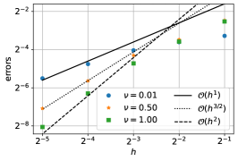
(a) Example 5.6, Matérn kernel.

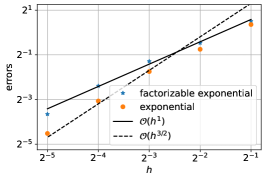
(b) Example 5.7, two exponential type covariances.

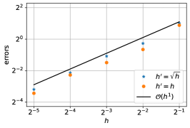
(c) Example 5.8, polynomial kernel with different resolutions of $\mathcal{T}_{h^{\prime}}$.

Figure 2. Strong error approximations for $X_{h,\Delta t}$.

Example 5.6 (Non-dominance of noise discretization errors).

In the case that $q$ is a Matérn kernel as in Example 5.1, we have $r_{1}+1\leq r_{2}\stackrel{{\scriptstyle\epsilon}}{{=}}\min(2,1+\nu)$ for $d\in\{2,3\}$, i.e., the noise discretization error does not dominate. This is true also for the Gaussian kernel of Example 5.2 and any $d$. It is also true for the first polynomial kernel of Example 5.3 when $d\in\{2,3\}$ (since then $r_{1}+1=r_{2}\stackrel{{\scriptstyle\epsilon}}{{=}}3/2$) and the second for any $d$ (since then $r_{1}+1\leq r_{2}\stackrel{{\scriptstyle\epsilon}}{{=}}2$).

We illustrate this in the simulation setting outlined above with $q$ of Matérn type with parameters $\rho=0.25,\sigma^{2}=10$ and $\nu\in\{0.01,0.5,1.0\}$. We let $X_{0}=b(x)=0$, pick Lipschitz functions $f(u,x)=f(u)=10^{-1}+u/(|u|+1)$, $g(u,x)=g(u)=u/(|u|+1)$ for $u\in\amsmathbb{R},x\in\mathcal{D}$, set $h^{\prime}=h$ and apply Neumann boundary conditions. The errors of Figure 2(a) are in line with the results of Theorem 4.4. See Figure 1(b) for a realization of $X_{h,\Delta t}$ with $\nu=0.5,h=2^{-7}$ and $\Delta t=10^{-3}$.

Example 5.7 (Dominance of noise discretization errors).

In $d=1$, the Matérn kernels yield $r_{1}+1\stackrel{{\scriptstyle\epsilon}}{{=}}\min(\nu,\theta,1)+1$ and $r_{2}\stackrel{{\scriptstyle\epsilon}}{{=}}\min(\nu+1/2,2)$, with dominant noise discretization error if $\nu\leq 1$ for Dirichlet and $\nu\leq 3/2$ for Neumann conditions. Similar conclusions hold for the first polynomial kernel of Example 5.3. This was demonstrated in a linear setting in [5], with different rates owing to errors being measured pointwise in space. Numerical experiments (not included in [5]) suggest this applies in our $L^{2}$ setting as well.

Factorizable kernels (Example 5.4) may exhibit dominant noise discretization errors even when $d>1$. We illustrate this with a numerical simulation comparing the exponential and the factorizable exponential kernel, both with $\rho=0.25$ and $\sigma^{2}=10$. We set $f(u)=10^{-1}$, $g(u)=1$ for $u\in\amsmathbb{R}$, $b(x)=10^{-1}(1,1)$ for $x\in\mathcal{D}$, equip $A$ with Dirichlet boundary conditions and otherwise follow the setting of Example 5.6. From Examples 5.1 and 5.4 we see that $r_{1}+1\stackrel{{\scriptstyle\epsilon}}{{=}}3/2$ for both the exponential and the factorizable exponential kernel, whereas $r_{2}\stackrel{{\scriptstyle\epsilon}}{{=}}3/2$ in the former case and $r_{2}\stackrel{{\scriptstyle\epsilon}}{{=}}1$ in the latter. The results (Figure 2(b)) align with Theorem 4.4.

One can potentially mitigate these issues by computing $I_{h}R_{\mathcal{S}\to\mathcal{D}}I_{h^{\prime}}\Delta\tilde{W}^{j}$ using finer meshes on $\mathcal{S}$ and $\mathcal{D}$ than the mesh used in (18). Efficient sampling methods could still maintain competitiveness of the approximation schemes. However, as FEniCS does not appear to support this, we do not explore this further.

Example 5.8 (Dominance of SPDE approximation error and noise sampling on a coarse mesh).

In our last example, we consider a non-smooth initial condition, namely $X_{0}(x)=3(-\log((x_{1}-0.5)^{2}+(x_{2}-0.5)^{2}))^{1/3}$, $x=(x_{1},x_{2})\in\mathcal{D}$. This function, while in $H^{1}(\mathcal{D})$, is not in $H^{1+\epsilon}(\mathcal{D})$ due to its discontinuity (cf. [18, page 1]). With $q$ as the second polynomial kernel of Example 5.3, $\sigma^{2}=10$, $f(u)=10^{-1}$, $g(u)=1$, $b(x)=0$, and Neumann boundary conditions for $A$, we find $r_{1}+1\stackrel{{\scriptstyle\epsilon}}{{=}}1$ and $r_{2}\stackrel{{\scriptstyle\epsilon}}{{=}}2$. Hence, the error stemming from the initial condition dominates the noise discretization error. We can therefore set $h^{\prime}=h^{1/2}$ and retain the same convergence rate as $h^{\prime}=h$, which is seen in Figure 2(c). Thus, for rough initial conditions, the computational effort can be further decreased without any essential loss of accuracy. Similarly, if we had a smooth initial condition with Dirichlet boundary conditions for $A$, we could set $h^{\prime}=h^{3/4}$ for analogous, albeit smaller, computational savings. This underscores the importance of noise discretization error analysis for efficient algorithm design.

Appendix A A fractional Sobolev norm error bound for piecewise linear finite element interpolants

Here we derive the bound $\|(I-I_{h})v\|_{W^{r}_{p}}\lesssim h^{\min(s-r,2)}\|v\|_{W^{s}_{p}}$ of Proposition 4.1, generalizing the results of [4] to $p\neq 2$ and $s<1$. For the Scott–Zhang interpolant, [9] treats this case, but as far as we know Proposition 4.1 cannot be inferred from this.

Proof of Proposition 4.1.

In this proof, we use for general $\mathcal{D}$ the notation

$$|u|_{W^{r,p}(\mathcal{D})}^{p}:=\sum_{|\alpha|=m}\int_{\mathcal{D}\times\mathcal{D}}\frac{|D^{\alpha}u(x)-D^{\alpha}u(y)|^{p}}{|x-y|^{d+p\sigma}}\,\mathrm{d}x\,\mathrm{d}y\quad r=m+\sigma,m\in\amsmathbb{N}_{0},\sigma\in(0,1).$$

Here $|\cdot|_{W^{r,p}(\mathcal{D})}^{p}$, $r\in\amsmathbb{N}$, is the usual Sobolev seminorm and the $L^{p}(\mathcal{D})$-norm for $r=0$.

Without loss of generality, let $s\leq 2$. We start with the cases $s\in(1,2]$ and $r=0$ or $r\in(1,1+1/p)\cap(1,s]$. The claim for $s\in(1,2]$, $r\in[0,1]$ then follows from real interpolation, see, e.g., [3, Theorem 3.1, Remark 3.3]. First note that for all $k\in\amsmathbb{N}_{0},\lambda\in(0,1)$, there is a $C<\infty$ such that for all $w\in W^{k+\lambda}_{p}$,

(26) $$|w|_{W^{k+\lambda}_{p}(\mathcal{D})}^{p}\leq C\sum_{|\alpha|=k}\sum_{T\in\mathcal{T}_{h}}\left(|D^{\alpha}w|^{p}_{W^{\lambda}_{p}(T)}+\int_{T}\frac{|D^{\alpha}w(x)|^{p}}{(\inf_{y\in\partial T}|x-y|)^{p\lambda}}\,\mathrm{d}x\right).$$

This is [4, Lemma 2.1] for $p=2$, the proof is analogous for $p\neq 2$. We also need an estimate on the reference simplex $\hat{T}$ with vertices $\hat{x}_{0}=(0,0,\ldots,0),\hat{x}_{1}=(1,\ldots,0)$, …$\hat{x}_{d}=(0,\ldots,d)$. For $\lambda\in[0,1/p)$, [18, Theorem 1.4.4.3] yields a $C<\infty$ such that

(27) $$\int_{\hat{T}}\frac{|w(x)|^{p}}{(\inf_{y\in\partial\hat{T}}|x-y|)^{p\lambda}}\,\mathrm{d}x\leq C\|w\|_{W^{\lambda}_{p}(\hat{T})}^{p},\qquad w\in W^{\lambda}_{p}(\hat{T}).$$

For each $T\in\mathcal{T}_{h}$, there is an affine transformation $\hat{T}\ni\hat{x}\mapsto B_{T}x+b_{T}\in T$. By regularity, there are $C_{1},C_{2}\in(0,\infty)$, that only depend on $\mathcal{D}$ (see [4, 8, 13]), such that

(28) $$C_{1}\mathrm{diam}(T)|\hat{x}|\leq|B_{T}\hat{x}|\leq C_{2}\mathrm{diam}(T)|\hat{x}|\leq C_{2}h|\hat{x}|,\quad\hat{x}\in\hat{T},T\in\mathcal{T}_{h}\text{ and }$$

(29) $$C_{1}\mathrm{diam}(T)^{d}\leq|\det B_{T}|\leq C_{2}\mathrm{diam}(T)^{d}\leq C_{2}h^{d},\quad T\in\mathcal{T}_{h}.$$

For quasiuniform $\mathcal{T}_{h}$, we also have corresponding lower bounds in terms of $h$.

Writing $v_{h}:=I_{h}v$, $\eqref{eq:thm:interpolation:1}$ yields $|v-v_{h}|_{W^{r}_{p}(\mathcal{D})}^{p}\lesssim\sum_{T\in\mathcal{T}_{h}}\mathrm{I}_{T}+\mathrm{II}_{T}$ for $r>1$, with

$$\mathrm{I}_{T}:=|v-v_{h}|^{p}_{W^{r}_{p}(T)}\text{ and }\mathrm{II}_{T}:=\sum_{|\alpha|=1}\int_{T}\frac{|D^{\alpha}v(x)-D^{\alpha}v_{h}(x)|^{p}}{(\inf_{y\in\partial T}|x-y|)^{p(r-1)}}\,\mathrm{d}x.$$

In the case that $r=0$, $\mathrm{II}_{T}:=0$. Let us write $e_{h}:=v-v_{h}$, $\hat{v}:=v(B_{T}\cdot+b_{T})$ and note that $\nabla\hat{v}_{h}=B_{T}^{*}\nabla v_{h}$, cf. [13, page 461]. Combining this, (28), (29) and equivalence of norms in $\amsmathbb{R}^{d}$, it follows by a scaling argument that for $r>1$

$$\mathrm{I}_{T} =|\det B_{T}|^{2}\int_{\hat{T}}\int_{\hat{T}}\frac{\sum_{|\alpha|=1}\left|D^{\alpha}e_{h}(B_{T}\hat{x}+b_{T})-D^{\alpha}e_{h}(B_{T}\hat{y}+b_{T})\right|^{p}}{|B_{T}(\hat{x}-\hat{y})|^{d+(r-1)p}}\,\mathrm{d}\hat{x}\,\mathrm{d}\hat{y}$$

$$\lesssim|\det B_{T}|^{2}\int_{\hat{T}}\int_{\hat{T}}\frac{\left|(B_{T}^{*})^{-1}\left(\nabla\hat{e}_{h}(\hat{x})-\nabla\hat{e}_{h}(\hat{y})\right)\right|^{p}}{|B_{T}(\hat{x}-\hat{y})|^{d+(r-1)p}}\,\mathrm{d}\hat{x}\,\mathrm{d}\hat{y}\lesssim\mathrm{diam}(T)^{d-rp}|\hat{e}_{h}|^{p}_{W^{r}_{p}(\hat{T})}.$$

For $r=0$, $\mathrm{I}_{T}$ is instead bounded by $|\det B_{T}|\|\hat{e}_{h}\|_{L^{p}(\hat{T})}^{p}\lesssim\mathrm{diam}(T)^{d}\|\hat{e}_{h}\|_{L^{p}(\hat{T})}^{p}$. In case $r>1$, we also use (27) with $\lambda=r-1<1/p$ to similarly deduce the estimate

$$\mathrm{II}_{T}\lesssim\mathrm{diam}(T)^{d-rp}\Big{(}|\hat{e}_{h}|^{p}_{W^{1}_{p}(\hat{T})}+|\hat{e}_{h}|^{p}_{W^{r}_{p}(\hat{T})}\Big{)}\lesssim\mathrm{diam}(T)^{d-rp}\|\hat{e}_{h}\|_{W^{r}_{p}(\hat{T})}^{p}.$$

Let $I_{h}^{\hat{T}}$ denote interpolation onto the set $\mathcal{P}_{1}(\hat{T})$ of linear polynomials on $\hat{T}$ and note that $\hat{v}_{h}=I_{h}^{\hat{T}}\hat{v}$. The Sobolev embedding $W^{s}_{p}(\hat{T})\hookrightarrow L^{\infty}(\hat{T})$ (see [18, Theorem 1.4.4.1]) yields $|\hat{v}_{h}|^{p}_{W^{1}_{p}(\hat{T})}\lesssim\|\hat{v}\|_{W^{s}_{p}(\hat{T})}^{p}$ after using equivalence of norms in $\amsmathbb{R}^{d}$ to see that

(30) $$|\hat{v}_{h}|^{p}_{W^{1}_{p}(\hat{T})}\lesssim\|\nabla\hat{v}_{h}\|_{L^{p}(\hat{T})}^{p}=(d!)^{-1}\Big{(}\sum_{j=1}^{d}|\hat{v}(\hat{x}_{0})-\hat{v}(\hat{x}_{j})|^{2}\Big{)}^{p/2}.$$

Similarly, $\|\hat{v}_{h}\|_{L^{p}(\hat{T})}\lesssim\|\hat{v}\|_{W^{s}_{p}(\hat{T})}$. Since $|f|_{W^{r}_{p}(\hat{T})}=0$ for $r>1$ and $f\in\mathcal{P}_{1}(\hat{T})$, this gives $I_{h}^{\hat{T}}\in\mathcal{L}(W^{s}_{p}(\hat{T}),W^{r}_{p}(\hat{T}))$ by real interpolation. These observations, the invariance of $I_{h}^{\hat{T}}$ on $\mathcal{P}_{1}(\hat{T})$ and the Bramble–Hilbert Lemma [13, Theorem 6.1] imply that

$$\|v-v_{h}\|_{W^{r}_{p}(\mathcal{D})}^{p}\lesssim\sum_{T\in\mathcal{T}_{h}}\mathrm{diam}(T)^{d-rp}\inf_{f\in\mathcal{P}_{1}}\|\hat{v}-f\|_{W^{s}_{p}(\hat{T})}^{p}\lesssim\sum_{T\in\mathcal{T}_{h}}\mathrm{diam}(T)^{d-rp}|\hat{v}|_{W^{s}_{p}(\hat{T})}^{p}.$$

This sum is bounded by $h^{(s-r)p}|v|^{p}_{W^{s}_{p}(\mathcal{D})}$ after applying this estimate to the summand:

$$|\det B_{T}^{-1}|^{2}\int_{T}\int_{T}\frac{\sum_{|\alpha|=1}\left|D^{\alpha}\hat{v}(B_{T}^{-1}(x-b_{T}))-D^{\alpha}\hat{v}(B_{T}^{-1}(y-b_{T}))\right|^{p}}{|B_{T}^{-1}(x-y)|^{d+(s-1)p}}\,\mathrm{d}x\,\mathrm{d}y$$

$$\quad\lesssim|\det B_{T}^{-1}|^{2}\int_{T}\int_{T}\frac{\left|B_{T}^{*}(\nabla v(x)-\nabla v(y))\right|^{p}}{|B_{T}^{-1}(x-y)|^{d+(s-1)p}}\,\mathrm{d}x\,\mathrm{d}y\lesssim\mathrm{diam}(T)^{sp-d}|v|^{p}_{W^{s}_{p}(T)}.$$

The proof for $s=1$ follows from interpolation of classical estimates, see [8, Remark 4.4.27]. The proof for $s<1$ and $r=0$ is similar to the case $r=0$ and $s>1$, except we apply (26) with $k=0$ and bound the infimum over $\mathcal{P}_{1}(\hat{T})$ when applying [13, Theorem 6.1] with the infimum over $\mathcal{P}_{0}(\hat{T})$, the space of constants on $\hat{T}$.

For $0<r=s<1$, we cannot invoke (27). Instead, scaling and (30) imply that

$$|v_{h}|_{W^{1}_{p}(\mathcal{D})}^{p} \lesssim\sum_{T\in\mathcal{T}_{h}}|\det B_{T}||(B_{T}^{*})^{-1}|^{p}|\nabla\hat{v}_{h}|_{L_{p}(\hat{T})}^{p}$$

$$\lesssim\sum_{T\in\mathcal{T}_{h}}|\det B_{T}||(B_{T}^{*})^{-1}|^{p}|\hat{v}|_{W^{s}_{p}(\hat{T})}^{p}$$

$$\lesssim\sum_{T\in\mathcal{T}_{h}}|\det B_{T}|^{-1}|(B_{T}^{*})^{-1}|^{p}|B_{T}^{-1}|^{-d-sp}|v|_{W^{s}_{p}(T)}^{p}\lesssim h^{(s-1)p}|v|_{W^{s}_{p}(\mathcal{D})},$$

using quasiuniformity in the last step. From this we obtain $\|e_{h}\|_{W^{1}_{p}}\lesssim h^{(s-1)}\|v\|_{W^{s}_{p}}$. Interpolating between this estimate and $\|e_{h}\|_{L^{p}}\lesssim h^{s}\|v\|_{W^{s}_{p}}$ completes the proof. ∎

References

- [1] E. J. Allen, S. J. Novosel, and Z. Zhang. Finite element and difference approximation of some linear stochastic partial differential equations. Stochastics Stochastics Rep., 64(1-2):117–142, 1998.
- [2] A. Barth and A. Lang. Simulation of stochastic partial differential equations using finite element methods. Stochastics, 84(2-3):217–231, 2012.
- [3] A. Behzadan and M. Holst. Multiplication in Sobolev spaces, revisited. Ark. Mat., 59(2):275–306, 2021.
- [4] F. Ben Belgacem and S. C. Brenner. Some nonstandard finite element estimates with applications to Poisson and Signorini problems. ETNA, Electron. Trans. Numer. Anal., 12:134–148, 2001.
- [5] F. E. Benth, G. Di Nunno, G. Lord, and A. Petersson. The heat modulated infinite dimensional heston model and its numerical approximation. Preprint at arXiv:2206.10166, June 2022.
- [6] A. Berlinet and C. Thomas-Agnan. Reproducing kernel Hilbert spaces in probability and statistics. Kluwer Academic Publishers, Boston, MA, 2004.
- [7] M. Boulakia, A. Genadot, and M. Thieullen. Simulation of SPDEs for excitable media using finite elements. J. Sci. Comput., 65(1):171–195, 2015.
- [8] S. C. Brenner and L. R. Scott. The mathematical theory of finite element methods, volume 15 of Texts in Applied Mathematics. Springer, New York, third edition, 2008.
- [9] P. j. Ciarlet. Analysis of the Scott-Zhang interpolation in the fractional order Sobolev spaces. J. Numer. Math., 21(3):173–180, 2013.
- [10] J. Cui and J. Hong. Strong and weak convergence rates of a spatial approximation for stochastic partial differential equation with one-sided Lipschitz coefficient. SIAM J. Numer. Anal., 57(4):1815–1841, 2019.
- [11] G. Da Prato and J. Zabczyk. Stochastic equations in infinite dimensions, volume 152 of Encyclopedia of mathematics and its applications. Cambridge University Press, Cambridge, second edition, 2014.
- [12] Q. Du and T. Zhang. Numerical approximation of some linear stochastic partial differential equations driven by special additive noises. SIAM J. Numer. Anal., 40(4):1421–1445, 2002.
- [13] T. Dupont and R. Scott. Polynomial approximation of functions in Sobolev spaces. Math. Comp., 34(150):441–463, 1980.
- [14] D. E. Edmunds and H. Triebel. Function spaces, entropy numbers, differential operators, volume 120 of Camb. Tracts Math. Cambridge: Cambridge Univ. Press, 1996.
- [15] H. Fujita and T. Suzuki. Evolution problems. Handbook of numerical analysis, II, pages 789 – 928. North-Holland, Amsterdam, 1991. Finite element methods. Part 1.
- [16] S. Geiger, G. Lord, and A. Tambue. Exponential time integrators for stochastic partial differential equations in 3d reservoir simulation. Comput. Geosci., 16(2):323–334, 2012.
- [17] I. G. Graham, F. Y. Kuo, D. Nuyens, R. Scheichl, and I. H. Sloan. Analysis of circulant embedding methods for sampling stationary random fields. SIAM J. Numer. Anal., 56(3):1871–1895, 2018.
- [18] P. Grisvard. Elliptic problems in nonsmooth domains, volume 24 of Monographs and studies in mathematics. Pitman (Advanced Publishing Program), Boston, MA, 1985.
- [19] A. Jentzen and M. Röckner. Regularity analysis for stochastic partial differential equations with nonlinear multiplicative trace class noise. Journal of Differential Equations, 252(1):114–136, 2012.
- [20] M. Kovács, S. Larsson, and F. Lindgren. Strong convergence of the finite element method with truncated noise for semilinear parabolic stochastic equations with additive noise. Numerical Algorithms, 53(2):309–320, Mar 2010.
- [21] M. Kovács, F. Lindgren, and S. Larsson. Spatial approximation of stochastic convolutions. J. Comput. Appl. Math., 235(12):3554–3570, 2011.
- [22] M. Kovács, A. Lang, and A. Petersson. Hilbert–Schmidt regularity of symmetric integral operators on bounded domains with applications to SPDE approximations. Stochastic Analysis and Applications, 2022. Published online.
- [23] R. Kruse. Strong and weak approximation of semilinear stochastic evolution equations, volume 2093 of Lecture notes in mathematics. Springer, Cham, 2014.
- [24] H. P. Langtangen and A. Logg. Solving PDEs in Python. The FEniCS tutorial I, volume 3 of Simula SpringerBriefs Comput. Cham: Springer Open, 2016.
- [25] G. J. Lord, C. E. Powell, and T. Shardlow. An introduction to computational stochastic PDEs. Cambridge Texts in Applied Mathematics. Cambridge University Press, 2014.
- [26] G. J. Lord and A. Tambue. A modified semi-implicit Euler-Maruyama scheme for finite element discretization of SPDEs with additive noise. Appl. Math. Comput., 332:105–122, 2018.
- [27] S. V. Lototsky and B. L. Rozovsky. Stochastic partial differential equations. Universitext. Springer, Cham, 2017.
- [28] A. Pietsch. Operator ideals. Licenced ed, volume 20. Elsevier (North-Holland), Amsterdam, 1980.
- [29] C. Prévôt and M. Röckner. A Concise Course on Stochastic Partial Differential Equations, volume 1905 of Lecture notes in mathematics. Springer, Berlin, 2007.
- [30] M. Riedle. Cylindrical Wiener processes. In Séminaire de Probabilités XLIII, Poitiers, France, Juin 2009., pages 191–214. Berlin: Springer, 2011.
- [31] M. L. Stein. Interpolation of spatial data. Springer Series in Statistics. Springer-Verlag, New York, 1999. Some theory for Kriging.
- [32] J. B. Walsh. Finite element methods for parabolic stochastic PDE’s. Potential Anal., 23(1):1–43, 2005.
- [33] H. Wendland. Scattered data approximation, volume 17 of Cambridge Monographs on Applied and Computational Mathematics. Cambridge University Press, Cambridge, 2005.
- [34] A. Yagi. Abstract parabolic evolution equations and their applications. Springer Monographs in Mathematics. Springer-Verlag, Berlin, 2010.
- [35] Y. Yan. Galerkin finite element methods for stochastic parabolic partial differential equations. SIAM J. Numer. Anal., 43(4):1363–1384, 2005.