The integrated perturbation theory for cosmological tensor fields II: Loop corrections

Abstract

In the previous paper [1], the nonlinear perturbation theory of cosmological density field is generalized to include the tensor-valued bias of astronomical objects, such as spins and shapes of galaxies and any other tensors of arbitrary ranks which are associated with objects that we can observe. We apply this newly developed method to explicitly calculate nonlinear power spectra and correlation functions both in real space and in redshift space. Multi-dimensional integrals that appear in loop corrections are reduced to combinations of one-dimensional Hankel transforms, thanks to the spherical basis of the formalism, and the final expressions are numerically evaluated in a very short time using an algorithm of the fast Fourier transforms such as FFTLog. As an illustrative example, numerical evaluations of loop corrections of the power spectrum and correlation function of the rank-2 tensor field are demonstrated with a simple model of tensor bias.

I Introduction

The large-scale structure (LSS) of the Universe, probed by galaxies and other astronomical observables such as weak lensing, 21cm emission and absorption lines and so forth, plays an essential role in cosmology. The LSS is complementary to the cosmic microwave background (CMB) radiation, which mainly probes the early stages of the Universe around the time of decoupling. The information contained in the temperature fluctuations in the CMB have been extracted in exquisite details, and the temperature and polarization maps obtained by Planck satellite determined the precise values of the cosmological parameters [2]. Beyond the cosmological information extracted from the CMB, the LSS offers a lot of opportunities to obtain further information of the Universe which is contained mainly in lower-redshift Universe. In addition, the representative values of the cosmological parameters determined by the Planck are obtained by combining the observational data of LSS, such as the scale of baryon acoustic oscillations (BAO) and weak lensing, as the CMB data alone has degeneracies among cosmological parameters. The acceleration of the universe due to dark energy is also an effect that can only be probed in the lower-redshift Universe.

While most of the physics in CMB is captured by the linear perturbation theory of fluctuations, the properties of LSS are more affected by nonlinear evolutions, as the scales of interest becomes smaller. On one hand, the physics of long-wavelength modes in the density fluctuations in the LSS can still be captured by the linear perturbation theory, and the amplitude of density fluctuations simply grows according to the linear growth factor. However, the number of independent modes of density fluctuations included in a survey is limited by the finiteness of the survey volume $V$, i.e., the number of independent Fourier modes with a wavenumber magnitude $k$ roughly scales as $\sim k^{3}V$ in three-dimensional surveys. On the other hand, short-wavelength modes are affected by nonlinear evolutions of density field, which mix up different scales of Fourier modes, and thus their analysis becomes much more difficult. The fully nonlinear evolutions can not be analytically solved because of the extreme mixture of modes, and extraction of the cosmological information from the fully nonlinear density field is difficult. While one can resort to the numerical simulations to solve the nonlinear evolutions, the information contents of initial condition and cosmology are largely lost in the nonlinearly evolved field [3], compared to the linearly evolved field.

The transition scales of the linear and nonlinear fields are roughly around $10$–$20\,h^{-1}\mathrm{Mpc}$ at the present time of $z=0$, and the transition scales become smaller at an earlier time of higher redshift. On the transition scales, although the linear theory does not quantitatively apply, the nonlinearity is still weak and the mixing of Fourier modes is not complicated enough. Only a countable number of modes are effectively mixed, and the nonlinear perturbation theory is applicable in such a situation. Therefore, the theory of nonlinear perturbation theory of density field [4] is expected to play an important role in the analysis of the LSS, in the era of large surveys in the near future when the sufficiently large number of Fourier modes on the transition scales are expected to be available. In addition, the density fluctuations even on large scales, which have been traditionally considered as the linear regime, are more or less affected by weak nonlinearity, and it is critically important to estimate such subtle effects in the era of precision cosmology. A representative example of the last case is the nonlinear smearing effects of the BAO in correlation functions of galaxies around $\sim 100\,h^{-1}\mathrm{Mpc}$ [5], which is used as a powerful standard ruler to probe the expansion history of the Universe and the nature of dark energy.

The higher-order perturbation theory beyond the linear theory have been extensively developed for matter distributions in past several decades [6, 7, 8, 9, 10, 11, 12, 13]. However, the distribution of matter is not the same as those of objects that we can observe, and the mass density field is dominated by the dark matter in the Universe. The bias between distributions of matter and observable objects is one of the most important concepts in understanding the large-scale structure of the Universe. In order that the nonlinear perturbation theory can be compared with observations, the effect of bias is an indispensable element that should be included in the theories with predictability of the observable Universe. There are many attempts to include the effect of bias in the nonlinear perturbation theory (for a recent review, see Ref. [14]). Understanding the bias from the first principle is extremely difficult because of the full nonlinearity of the problem and extremely complicated astrophysical processes in the galaxy formation, and so forth.

The concept of bias has usually been discussed in the context of number density fields of astronomical objects such as galaxies, as probes of the underlying matter density field. In this case, the bias corresponds to a function, or more properly a functional, of the underlying mass density field to give a number density field of the biased objects. Thus the function(al) of the bias has a scalar value in accordance with that the density of biased objects is a scalar field. In the previous work of Paper I [1], the concept of bias in the nonlinear perturbation theory is generalized to the case that the bias is given by a tensor field. The number densities of objects are not the only probes of the density fields in the LSS. For example, galaxy spins and shapes are in principle determined by the mass density fields through, e.g., tidal gravitational forces, and other physical quantities. Recently interests in statistics of the galaxy sizes and shapes, or intrinsic alignments, are growing as probes of the LSS of the Universe [15, 16, 17, 18, 19], and analytical modelings of galaxy shape statistics by the nonlinear perturbation theory have also been introduced [20, 21, 22, 23, 24].

Motivated by these recent developments, we generalize the nonlinear perturbation theory to predict statistics of biased fields with an arbitrary rank of tensor in Paper I [1]. We adopt the spherical decomposition of the tensor field, which plays an important role in the formalism. This method of decomposition has been already adopted in the perturbation theory in literature to investigate the clustering of density peaks [25] and galaxy shapes [23]. In the last two references, the coordinates system of the spherical basis is chosen so that the third axis is aligned with a radial direction of the correlation function, or a direction of wavevector of perturbations in Fourier space. In contrast, we do not fix the coordinates system in the spherical basis, and explicitly keep the rotational covariance apparent throughout the formulation. The basic formalism to calculate the power spectrum and higher-order spectra of tensor fields of arbitrary ranks by the nonlinear perturbation theory to arbitrary orders is described in Paper I.

Many different methods have been considered in the literature to include the bias in the nonlinear perturbation theory [14]. Most methods rely on a local or semi-local ansatz of the bias function which relates the mass density field and the biased density field. The locality or semi-locality of the relation is given by either Eulerian or Lagrangian space of the density field. However, (semi-)local biases in Eulerian and Lagrangian spaces are not compatible with each other in general, because the dynamically nonlinear evolution by gravity is essentially nonlocal. Therefore, the bias relation should be given by a nonlocal functional, in either Eulerian or Lagrangian space, and the (semi-)local ansatz are approximations to the reality. A general formulation to systematically incorporate the nonlocal bias into the nonlinear perturbation theory is provided by the integrated perturbation theory (iPT) [26, 27]. The local and semi-local ansatz of the bias can also be derived from this formulation by restricting the form of bias functional in the class of local or semi-local function. Moreover, the iPT also provides a natural way of including the effect of redshift space distortions, which should be taken into account for predicting observable statistics in redshift surveys. Our formulation of Paper I is built upon and generalizes the method of iPT and establishes a nonlinear perturbation theory of tensor fields in general. Paper I describes the basic formulation of the theory and gives some results of lowest-order approximations of the perturbation theory.

In this second paper of the series, we apply the formulation of Paper I to concretely calculate the one-loop corrections of the perturbation theory. The strategy of the calculation is fairly straightforward according to Paper I. Some techniques are introduced to reduce the higher-dimensional integrals to the lower ones, which are generalizations of an existing method using a fast Fourier transform applied to the nonlinear perturbation theory [28]. In particular, all the necessary integrations to evaluate the one-loop corrections in the perturbation theory with the (semi-)local models of tensor bias reduce to essentially one-dimensional Hankel transforms. As an illustrative example, we calculate the power spectrum and correlation function with one-loop corrections for a simple model of a rank-2 tensor which is biased from spatially second derivatives of the gravitational potential in Lagrangian space.

This paper is organized as follows. In Sec. II, the propagators, elements of the nonlinear perturbation theory, in the spherical basis of our formalism are calculated, up to necessary orders for evaluating one-loop corrections of the power spectrum and correlation function. In Sec. III, our main result, the one-loop approximations of the power spectra of the tensor field are explicitly derived in analytic forms, both in real space and in redshift space. In Sec. IV, a simple example of the tensor bias with a semi-local model is explicitly calculated and numerically evaluated. Conclusions are given in Sec. V. In Appendix A, a formal expression of the all-order power spectrum of the tensor field is derived beyond the one-loop approximation.

II Propagators of tensor fields and loop corrections

The fundamental formulation of the iPT of tensor fields is described in Paper I [1]. One of the essential ingredients of the theory is the evaluation of propagators, with which statistics of tensor fields, such as the power spectrum, bispectrum, correlation functions, etc. are represented. Several examples in relatively simple cases with lowest-order approximation are explicitly derived in Paper I. In this section, we further derive the propagators which is required to evaluate next-order approximation with loop corrections. We cite many equations from Paper I, which readers are assumed to have in hand.

II.1 Invariant propagators

The propagators of tensor fields can be represented by rotationally invariant functions as well as the renormalized bias functions as extensively explained in Paper I. First we summarize the essential equations and introduce various quantities and functions which are used in later sections. The concepts of propagators and renormalized bias functions are explained in detail in Paper I. The details of the definitions are not explained here. In short, they are response functions of the nonlinear evolutions from the initial density field. We summarize their properties below which are essential to derive main equations in later sections of this paper.

II.1.1 Real space

The propagators up to the second order are represented by invariant functions as

$$\hat{\Gamma}^{(1)}_{Xlm}(\bm{k})=\frac{(-1)^{l}}{\sqrt{2l+1}}\,\hat{\Gamma}^{(1)}_{Xl}(k)C_{lm}(\hat{\bm{k}}),$$ (1)

for the first order, and

$$\hat{\Gamma}^{(2)}_{Xlm}(\bm{k}_{1},\bm{k}_{2})=\sum_{l_{1},l_{2}}\hat{\Gamma}^{(2)\,l}_{Xl_{1}l_{2}}(k_{1},k_{2})X^{l_{1}l_{2}}_{lm}(\hat{\bm{k}}_{1},\hat{\bm{k}}_{2}),$$ (2)

for the second order. In the above equations, the index $X$ specifies the class of tensor-valued objects in general, such as the density (scalar), angular momentum (vector) or shape (tensors) of certain type of galaxies etc. The functions $\hat{\Gamma}^{(1)}_{Xl}(k)$ and $\hat{\Gamma}^{(2)\,l}_{Xl_{1}l_{2}}(k_{1},k_{2})$ are the invariant propagators which are invariant under the coordinates rotations. We use the spherical harmonics with Racah’s normalization,

$$C_{lm}(\theta,\phi)\equiv\sqrt{\frac{4\pi}{2l+1}}Y_{lm}(\theta,\phi)=\sqrt{\frac{(l-m)!}{(l+m)!}}P_{l}^{m}(\cos\theta)\,e^{im\phi},$$ (3)

instead of standard normalization of spherical harmonics $Y_{lm}$. The argument of the spherical harmonics is alternatively represented by a unit vector $\bm{n}$, instead of the corresponding angular coordinates $(\theta,\phi)$ of $\bm{n}$. In the above notation, the Condon-Shortley phase is included in the associated Legendre polynomials $P_{l}^{m}$ as

$$P_{l}^{m}(x)=\frac{(-1)^{m}}{2^{l}\,l!}\left(1-x^{2}\right)^{m/2}\frac{d^{l+m}}{dx^{l+m}}\left(1-x^{2}\right)^{l}.$$ (4)

The function of the last factor in Eq. (2) is the bipolar spherical harmonics with an appropriate normalization,

$$X^{l_{1}l_{2}}_{lm}(\bm{n}_{1},\bm{n}_{2})=\left(l\,l_{1}\,l_{2}\right)_{m}^{\phantom{m}m_{1}m_{2}}C_{l_{1}m_{1}}(\bm{n}_{1})C_{l_{2}m_{2}}(\bm{n}_{2}),$$ (5)

where azimuthal indices $m_{1}$ and $m_{2}$ are summed over from $-l_{1}$ to $+l_{1}$ and from $-l_{2}$ to $+l_{2}$, respectively, without summation symbols following the Einstein convention, and

$$\left(l\,l_{1}\,l_{2}\right)_{m}^{\phantom{m}m_{1}m_{2}}=(-1)^{m_{1}+m_{2}}\begin{pmatrix}l&l_{1}&l_{2}\\ m&-m_{1}&-m_{2}\end{pmatrix}.$$ (6)

is a Wigner’s $3j$-symbol.

It is convenient to use the metric tensor of spherical basis, defined by

$$g_{(l)}^{mm^{\prime}}=g^{(l)}_{mm^{\prime}}=(-1)^{m}\delta_{m,-m^{\prime}},$$ (7)

where $\delta_{m,-m^{\prime}}$ is the Kronecker’s symbol which is unity when $m+m^{\prime}=0$ and is zero otherwise. With this notation, Eq. (6) is represented by

$$\left(l\,l_{1}\,l_{2}\right)_{m}^{\phantom{m}m_{1}m_{2}}=g_{(l)}^{m_{1}m_{1}^{\prime}}g_{(l)}^{m_{2}m_{2}^{\prime}}\left(l\,l_{2}\,l_{3}\right)_{mm_{1}^{\prime}m_{2}^{\prime}},$$ (8)

where

$$\left(l_{1}\,l_{2}\,l_{3}\right)_{m_{1}m_{2}m_{3}}=\begin{pmatrix}l_{1}&l_{2}&l_{3}\\ m_{1}&m_{2}&m_{3}\end{pmatrix}$$ (9)

is the usual $3j$-symbol, and Einstein’s summation convention for the azimuthal indices $m$, $m_{1}$, etc. are assumed throughout this paper, unless otherwise stated. The two spherical metric tensors satisfy $g_{(l)}^{mm^{\prime\prime}}g^{(l)}_{m^{\prime\prime}m^{\prime}}=\delta^{m}_{m^{\prime}}$. Similarly to Eq. (8), we understand that the azimuthal indices can be raised or lowered by the spherical metric tensor, for example,

$$\left(l_{1}\,l_{2}\,l_{3}\right)_{m_{1}m_{2}}^{\phantom{m_{1}m_{2}}m_{3}}=g_{(l)}^{m_{3}m_{3}^{\prime}}\left(l_{1}\,l_{2}\,l_{3}\right)_{m_{1}m_{2}m_{3}^{\prime}},$$ (10)

and so forth.

With the above notation, the complex conjugate of the spherical harmonics is represented by

$$C^{*}_{lm}(\bm{n})=g_{(l)}^{mm^{\prime}}C_{lm^{\prime}}(\bm{n}),$$ (11)

and similarly that of the bipolar spherical harmonics is represented by

$$X^{l_{1}l_{2}*}_{lm}(\hat{\bm{k}}_{1},\hat{\bm{k}}_{2})=(-1)^{l_{1}+l_{2}+l}g_{(l)}^{mm^{\prime}}X^{l_{1}l_{2}}_{lm^{\prime}}(\hat{\bm{k}}_{1},\hat{\bm{k}}_{2}).$$ (12)

The orthonormality relation of spherical harmonics is given by

$$\int\frac{d^{2}n}{4\pi}\,C_{lm}^{*}(\bm{n})C_{l^{\prime}m^{\prime}}(\bm{n})=\frac{\delta_{ll^{\prime}}}{2l+1}\delta^{m}_{m^{\prime}},$$ (13)

and those of bipolar spherical harmonics is given by

$$\int\frac{d^{2}\hat{k}_{1}}{4\pi}\frac{d^{2}\hat{k}_{2}}{4\pi}X^{l_{1}l_{2}*}_{lm}(\hat{\bm{k}}_{1},\hat{\bm{k}}_{2})X^{l_{1}^{\prime}l_{2}^{\prime}}_{l^{\prime}m^{\prime}}(\hat{\bm{k}}_{1},\hat{\bm{k}}_{2})\\ =\frac{\delta_{ll^{\prime}}\delta_{l_{1}l_{1}^{\prime}}\delta_{l_{2}l_{2}^{\prime}}\delta^{\triangle}_{l_{1}l_{2}l}}{(2l+1)(2l_{1}+1)(2l_{2}+1)}\delta^{m}_{m^{\prime}},$$ (14)

where $\delta^{\triangle}_{l_{1}l_{2}l}$ is unity when the set of integers $(l_{1},l_{2},l)$ satisfies triangle inequality $|l_{1}-l_{2}|\leq l\leq l_{1}+l_{2}$, and is zero otherwise.

The invariant propagator of the second order satisfies an interchange symmetry,

$$\hat{\Gamma}^{(2)\,l}_{Xl_{2}l_{1}}(k_{2},k_{1})=(-1)^{l_{1}+l_{2}+l}\,\hat{\Gamma}^{(2)\,l}_{Xl_{1}l_{2}}(k_{1},k_{2}).$$ (15)

The above expansions of Eqs. (1) and (2) are inverted by the above orthonormality relations, and we have

$$\hat{\Gamma}^{(1)}_{Xl}(k)=(-1)^{l}\sqrt{2l+1}\,g_{(l)}^{mm^{\prime}}\int\frac{d^{2}\hat{k}}{4\pi}\,\hat{\Gamma}^{(1)}_{Xlm}(\bm{k})C_{lm^{\prime}}(\hat{\bm{k}})$$ (16)

for the first-order propagator, and

$$\hat{\Gamma}^{(2)\,l}_{Xl_{1}l_{2}}(k_{1},k_{2})=(2l_{1}+1)(2l_{2}+1)\,g_{(l)}^{mm^{\prime}}\\ \times\int\frac{d^{2}\hat{k}_{1}}{4\pi}\frac{d^{2}\hat{k}_{2}}{4\pi}\,\hat{\Gamma}^{(2)}_{Xlm}(\bm{k}_{1},\bm{k}_{2})X^{l_{1}l_{2}}_{lm^{\prime}}(\hat{\bm{k}}_{1},\hat{\bm{k}}_{2})$$ (17)

for the second-order propagator. In practice, one can always represent the propagators with polypolar spherical harmonics in the form of Eqs. (1) and (2), and can readily read off the expression of the invariant functions from the results.

II.1.2 Redshift space

In redshift space, the propagators also depend on the direction of line of sight. We can decompose the dependence on the line of sight in spherical harmonics, together with the dependencies on the directions of wavevectors. For the first-order propagator in redshift space, we have

$$\hat{\Gamma}^{(1)}_{Xlm}(\bm{k};\hat{\bm{z}};k,\mu)=\sum_{l_{z},l_{1}}\hat{\Gamma}^{(1)\,l\,l_{z}}_{Xl_{1}}(k,\mu)X^{l_{z}l_{1}}_{lm}(\hat{\bm{z}},\hat{\bm{k}}),$$ (18)

where $\hat{\bm{z}}$ is the direction to the line of sight. We assume the distant-observer approximation, and the direction to the line of sight is fixed in space. Unlike the common practice, we do not fix the line of sight in the third direction of the coordinates, but allow to point in any direction. In the above expression, the direction cosine to the line of sight, $\mu\equiv\hat{\bm{z}}\cdot\hat{\bm{k}}$, is included. This dependence is not necessarily included there, because the angular dependence on the left-hand side (lhs) of the equation can be completely expanded into spherical harmonics (Paper I). However, it is sometimes convenient to leave some part of the dependence in the form of the direction cosine $\mu$ between the line of sight and the direction of wavevector. Which part of the dependence is kept unexpanded is arbitrary. Even though the arguments $k$ and $\mu$ of the propagator on the lhs of Eq. (18) is a function of $\bm{k}$ and $\hat{\bm{z}}$, the explicit arguments of $k$ and $\mu$ specify which parts of the angular dependence in these parameters are unexpanded in the spherical harmonics on the right-hand side (rhs).

For the second-order propagator in redshift space, we have

$$\hat{\Gamma}^{(2)}_{Xlm}(\bm{k}_{1},\bm{k}_{2};\hat{\bm{z}};k,\mu)\\ =\sum_{l_{z},l_{1},l_{2},L}\hat{\Gamma}^{(2)\,l\,l_{z};L}_{Xl_{1}l_{2}}(k_{1},k_{2};k,\mu)X^{l_{z}l_{1}l_{2}}_{L;lm}(\hat{\bm{z}},\hat{\bm{k}}_{1},\hat{\bm{k}}_{2}),$$ (19)

where

$$X^{l_{1}l_{2}l_{3}}_{L;lm}(\bm{n}_{1},\bm{n}_{2},\bm{n}_{3})=(-1)^{L}\sqrt{2L+1}\left(l\,l_{1}\,L\right)_{m}^{\phantom{m}m_{1}M}\left(L\,l_{2}\,l_{3}\right)_{M}^{\phantom{M}m_{2}m_{3}}\\ \times C_{l_{1}m_{1}}(\bm{n}_{1})C_{l_{2}m_{2}}(\bm{n}_{2})C_{l_{3}m_{3}}(\bm{n}_{3})$$ (20)

is the tripolar spherical harmonics with an appropriate normalization. In the argument of propagators, the variables $k=|\bm{k}|$ and $\mu=\hat{\bm{z}}\cdot\hat{\bm{k}}$ are given by the total wavevector $\bm{k}=\bm{k}_{1}+\bm{k}_{2}$, which is optionally allowed to be included, because keeping the angular dependencies in these variables significantly simplify the analytic calculations. The invariant propagator of the second order satisfies an interchange symmetry,

$$\hat{\Gamma}^{(2)\,l\,l_{z};L}_{Xl_{2}l_{1}}(k_{2},k_{1};k,\mu)=(-1)^{l_{1}+l_{2}+L}\hat{\Gamma}^{(2)\,l\,l_{z};L}_{Xl_{1}l_{2}}(k_{1},k_{2};k,\mu).$$ (21)

The complex conjugate of the tripolar spherical harmonics is given by

$$X^{l_{1}l_{2}l_{3}*}_{lm}(\bm{n}_{1},\bm{n}_{2},\bm{n}_{3})=(-1)^{l+l_{1}+l_{2}+l_{3}}g_{(l)}^{mm^{\prime}}X^{l_{1}l_{2}l_{3}}_{lm^{\prime}}(\bm{n}_{1},\bm{n}_{2},\bm{n}_{3}),$$ (22)

and the orthonormality relation is given by

$$\int\frac{d^{2}n_{1}}{4\pi}\frac{d^{2}n_{2}}{4\pi}\frac{d^{2}n_{3}}{4\pi}X^{l_{1}l_{2}l_{3}}_{L;lm}(\bm{n}_{1},\bm{n}_{2},\bm{n}_{3})X^{l_{1}^{\prime}l_{2}^{\prime}l_{3}^{\prime}}_{L^{\prime};l^{\prime}m^{\prime}}(\bm{n}_{1},\bm{n}_{2},\bm{n}_{3})\\ =\frac{(-1)^{l+l_{1}+l_{2}+l_{3}}\delta_{ll^{\prime}}\delta_{l_{1}l_{1}^{\prime}}\delta_{l_{2}l_{2}^{\prime}}\delta_{l_{3}l_{3}^{\prime}}\delta_{LL^{\prime}}\delta^{\triangle}_{l\,l_{1}L}\delta^{\triangle}_{Ll_{2}l_{3}}}{(2l+1)(2l_{1}+1)(2l_{2}+1)(2l_{3}+1)}g^{(l)}_{mm^{\prime}}.$$ (23)

Applying the above orthonormality relations for bipolar and tripolar spherical harmonics, Eqs. (14) and (23), the first- and second-order propagators in redshift space of Eqs. (18) and (19) are inverted as

$$\hat{\Gamma}^{(1)\,l\,l_{z}}_{Xl_{1}}(k,\mu)=(2l_{z}+1)(2l_{1}+1)\,g_{(l)}^{mm^{\prime}}\\ \times\int\frac{d^{2}\hat{z}}{4\pi}\frac{d^{2}\hat{k}}{4\pi}\,\hat{\Gamma}^{(1)}_{Xlm}(\bm{k};\hat{\bm{z}};k,\mu)X^{l_{z}l_{1}}_{lm^{\prime}}(\hat{\bm{z}},\hat{\bm{k}})$$ (24)

for the first-order propagator, and

$$\hat{\Gamma}^{(2)\,l\,l_{z};L}_{Xl_{1}l_{2}}(k_{1},k_{2};k,\mu)=(2l_{z}+1)(2l_{1}+1)(2l_{2}+1)\,g_{(l)}^{mm^{\prime}}\\ \times\int\frac{d^{2}\hat{z}}{4\pi}\frac{d^{2}\hat{k}_{1}}{4\pi}\frac{d^{2}\hat{k}_{2}}{4\pi}\,\hat{\Gamma}^{(2)}_{Xlm}(\bm{k}_{1},\bm{k}_{2};\hat{\bm{z}};k,\mu)X^{l_{z}l_{1}l_{2}}_{L;lm^{\prime}}(\hat{\bm{z}},\hat{\bm{k}}_{1},\hat{\bm{k}}_{2})$$ (25)

for the second-order propagator. In the above equations, the angular integrations on the rhs in variables $k$ and $\mu$ are formally fixed, as if they do not depends on $\hat{\bm{k}}$, $\hat{\bm{k}}_{1}$, $\hat{\bm{k}}_{2}$ and $\hat{\bm{z}}$. The expressions of Eqs. (24) and (25) should be considered as formal, and should only be used in order to invert the expansions of Eqs. (18) and (19), formally fixing the variables $k$ and $\mu$ on both sides of the equations.

In practice, one can always represent the propagators with polypolar spherical harmonics in the form of Eqs. (18) and (19), and can readily read off the expression of the invariant functions from the results. The invariant propagators in real space, Eqs. (16) and (17), correspond to $\hat{\Gamma}^{(1)}_{Xl}(k)=\hat{\Gamma}^{(1)\,l0}_{Xl}(k)$, $\hat{\Gamma}^{(2)\,l}_{Xl_{1}l_{2}}(k_{1},k_{2})=\hat{\Gamma}^{(2)\,l\,0;l}_{Xl_{1}l_{2}}(k_{1},k_{2})$ when the propagators do not contain redshift-space distortions.

II.2 First-order propagators with loop corrections

II.2.1 The propagators of integrated perturbation theory

The first-order and second-order propagators, $\hat{\Gamma}^{(1)}_{Xlm}(\bm{k})$ and $\hat{\Gamma}^{(2)}_{Xlm}(\bm{k}_{1},\bm{k}_{2})$ are evaluated by the iPT. The results are given by (Paper I)

$$\hat{\Gamma}_{Xlm}^{(1)}(\bm{k})=c_{Xlm}^{(1)}(\bm{k})+\left[\bm{k}\cdot\bm{L}_{1}(\bm{k})\right]c_{Xlm}^{(0)}\\ +\int\frac{d^{3}p}{(2\pi)^{3}}P_{\mathrm{L}}(p)\biggl{\{}\left[\bm{k}\cdot\bm{L}_{1}(-\bm{p})\right]c_{Xlm}^{(2)}(\bm{k},\bm{p})\\ +\left[\bm{k}\cdot\bm{L}_{1}(-\bm{p})\right]\left[\bm{k}\cdot\bm{L}_{1}(\bm{k})\right]c_{Xlm}^{(1)}(\bm{p})\\ +\left[\bm{k}\cdot\bm{L}_{2}(\bm{k},-\bm{p})\right]c_{Xlm}^{(1)}(\bm{p})\\ +\frac{1}{2}\left[\bm{k}\cdot\bm{L}_{3}(\bm{k},\bm{p},-\bm{p})\right]c_{Xlm}^{(0)}\\ +\left[\bm{k}\cdot\bm{L}_{1}(\bm{p})\right]\left[\bm{k}\cdot\bm{L}_{2}(\bm{k},-\bm{p})\right]c_{Xlm}^{(0)}\biggr{\}}$$ (26)

for the first-order propagator, and

$$\hat{\Gamma}^{(2)}_{Xlm}(\bm{k}_{1},\bm{k}_{2})=c^{(2)}_{Xlm}(\bm{k}_{1},\bm{k}_{2})\\ +\left[\bm{k}_{12}\cdot\bm{L}_{1}(\bm{k}_{1})\right]c^{(1)}_{Xlm}(\bm{k}_{2})+\left[\bm{k}_{12}\cdot\bm{L}_{1}(\bm{k}_{2})\right]c^{(1)}_{Xlm}(\bm{k}_{1})\\ +\left\{\left[\bm{k}_{12}\cdot\bm{L}_{1}(\bm{k}_{1})\right]\left[\bm{k}_{12}\cdot\bm{L}_{1}(\bm{k}_{2})\right]+\bm{k}_{12}\cdot\bm{L}_{2}(\bm{k}_{1},\bm{k}_{2})\right\}c^{(0)}_{Xlm}.$$ (27)

for the second-order propagator. It is sufficient to include one-loop corrections only in the first-order propagator $\hat{\Gamma}^{(1)}_{Xlm}$ and not in the second-order propagator $\hat{\Gamma}^{(2)}_{Xlm}$, because the second-order propagator always appear with loop integrals in evaluating the nonlinear power spectrum [26, 27].

In the above equations, $c^{(0)}_{X}$, $c^{(1)}_{Xlm}(\bm{k})$, $c^{(2)}_{Xlm}(\bm{k}_{1},\bm{k}_{2})$ are the renormalized bias functions, which are determined from complicated physics involving nonlinear dynamics of galaxy formation, etc., and the definitions of these functions are given in Paper I. The vector functions $\bm{L}_{n}(\bm{k}_{1},\ldots,\bm{k}_{n})$ are the kernel functions of the Lagrangian perturbation theory. In real space, they are explicitly given by [29, 30]

$$\bm{L}_{1}(\bm{k})=\frac{\bm{k}}{k^{2}},$$ (28)

$$\bm{L}_{2}(\bm{k}_{1},\bm{k}_{2})=\frac{3}{7}\frac{\bm{k}_{12}}{{k_{12}}^{2}}\left[1-\left(\frac{\bm{k}_{1}\cdot\bm{k}_{2}}{k_{1}k_{2}}\right)^{2}\right],$$ (29)

$$\bm{L}_{3}(\bm{k}_{1},\bm{k}_{2},\bm{k}_{3})=\frac{1}{3}\left[\tilde{\bm{L}}_{3}(\bm{k}_{1},\bm{k}_{2},\bm{k}_{3})+\mathrm{cyc.}\right],$$ (30)

$$\tilde{\bm{L}}_{3}(\bm{k}_{1},\bm{k}_{2},\bm{k}_{3})$$

$$\quad=\frac{\bm{k}_{123}}{{k_{123}}^{2}}\left\{\frac{5}{7}\left[1-\left(\frac{\bm{k}_{1}\cdot\bm{k}_{2}}{k_{1}k_{2}}\right)^{2}\right]\left[1-\left(\frac{\bm{k}_{12}\cdot\bm{k}_{3}}{{k}_{12}k_{3}}\right)^{2}\right]\right.$$

$$\qquad\quad\left.-\frac{1}{3}\left[1-3\left(\frac{\bm{k}_{1}\cdot\bm{k}_{2}}{k_{1}k_{2}}\right)^{2}+\,2\frac{(\bm{k}_{1}\cdot\bm{k}_{2})(\bm{k}_{2}\cdot\bm{k}_{3})(\bm{k}_{3}\cdot\bm{k}_{1})}{{k_{1}}^{2}{k_{2}}^{2}{k_{3}}^{2}}\right]\right\}$$

$$\qquad+\frac{3}{7}\frac{\bm{k}_{123}}{{k_{123}}^{2}}\times\frac{(\bm{k}_{1}\times\bm{k}_{23})(\bm{k}_{1}\cdot\bm{k}_{23})}{{k_{1}}^{2}{k_{23}}^{2}}\left[1-\left(\frac{\bm{k}_{2}\cdot\bm{k}_{3}}{k_{2}k_{3}}\right)^{2}\right],$$ (31)

where $\bm{k}_{12}=\bm{k}_{1}+\bm{k}_{2}$, $\bm{k}_{123}=\bm{k}_{1}+\bm{k}_{2}+\bm{k}_{3}$, and $+\,\mathrm{cyc.}$ corresponds to the two terms which are added with cyclic permutations of each previous term. Weak dependencies on the time in the kernels are neglected [32, 31]. In Ref. [31], complete expressions of the displacement kernels of LPT up to the seventh order including the transverse parts are explicitly given, together with a general way of recursively deriving the kernels including weak dependencies on the time in general cosmology and subleading growing modes. The redshift-space distortions can be simply taken into account as well in the Lagrangian perturbation theory, just replacing the displacement kernel in real space given above with the linearly mapped kernels [33]

$$\bm{L}_{n}\rightarrow\bm{L}^{\mathrm{s}}_{n}=\bm{L}_{n}+nf\left(\hat{\bm{z}}\cdot\bm{L}_{n}\right)\hat{\bm{z}},$$ (32)

where $f=d\ln D/d\ln a=\dot{D}/HD$ is the linear growth rate, $D(t)$ is the linear growth factor, $a(t)$ is the scale factor, and $H(t)=\dot{a}/a$ is the time-dependent Hubble parameter. The distant-observer approximation is assumed in redshift space and the unit vector $\hat{\bm{z}}$ denotes the line-of-sight direction, as already mentioned above.

The first-order propagators $\Gamma^{(1)}_{Xlm}$ in the lowest order approximation, i.e., without loop corrections, are explicitly derived in Paper I. The results are given by

$$\hat{\Gamma}^{(1)}_{Xl}(k)=c^{(1)}_{Xl}(k)+\delta_{l0}c^{(0)}_{X}$$ (33)

in real space, and

$$\hat{\Gamma}^{(1)l\,l_{z}}_{Xl_{1}}(k,\mu)=\delta_{l_{z}0}\delta_{l_{1}l}\left[c^{(1)}_{Xl}(k)+\delta_{l0}(1+f\mu^{2})c^{(0)}_{X}\right].$$ (34)

in redshift space. In the last expression in redshift space, the dependence on the direction cosine $\mu$ is kept unexpanded into spherical harmonics. An another expression with complete expansion is given in Paper I. Below we consider the generalization of the lowest-order results, and derive necessary propagators for evaluating one-loop corrections in the nonlinear power spectrum.

II.2.2 Real space

In the expression of propagators, Eqs. (26)–(31), many scalar products between pairs of wavevectors appear, and they can always be represented by the spherical harmonics by applying the addition theorem of the spherical harmonics,

$$P_{l}(\bm{n}\cdot\bm{n}^{\prime})=C_{lm}^{*}(\bm{n})C_{lm}(\bm{n}^{\prime}),$$ (35)

where $\bm{n}$, $\bm{n}^{\prime}$ are normal vectors, and $P_{l}(x)$ is the Legendre polynomial. Einstein’s summation convention for the index $m$ is applied as before. For example, we have

$$\bm{k}\cdot\bm{L}_{1}(\pm\bm{p})=\pm\frac{\bm{k}\cdot\bm{p}}{p^{2}}=\pm\frac{k}{p}C_{1m}^{*}(\hat{\bm{k}})C_{1m}(\hat{\bm{p}}).$$ (36)

Similarly the all the directional dependencies on the wavevectors are expanded into the spherical harmonics. In the such reductions, representing simple polynomials by Legendre polynomials, such as

$$1=P_{0}(x),\ \ x=P_{1}(x),\ \ x^{2}=\frac{1}{3}P_{0}(x)+\frac{2}{3}P_{2}(x),$$

$$x^{3}=\frac{3}{5}P_{1}(x)+\frac{2}{5}P_{3}(x),\ \ x^{4}=\frac{1}{5}P_{0}(x)+\frac{4}{7}P_{2}(x)+\frac{8}{35}P_{4}(x),$$ (37)

are useful.

A non-polynomial factor $|\bm{k}\pm\bm{p}|^{-2}$ appears in the one-loop integrations in Eq. (26) through the factors

$$\bm{k}\cdot\bm{L}_{2}(\bm{k},-\bm{p}) =\frac{3}{7}\frac{k^{2}-\bm{k}\cdot\bm{p}}{|\bm{k}-\bm{p}|^{2}}\left[1-(\hat{\bm{k}}\cdot\hat{\bm{p}})^{2}\right],$$ (38)

$$\bm{k}\cdot\bm{L}_{3}(\bm{k},\bm{p},-\bm{p}) =\frac{5}{21}\left(\frac{k^{2}}{|\bm{k}-\bm{p}|^{2}}+\frac{k^{2}}{|\bm{k}+\bm{p}|^{2}}\right)\left[1-(\hat{\bm{k}}\cdot\hat{\bm{p}})^{2}\right]^{2}.$$ (39)

The directional dependence of this non-polynomial factor can also be expanded by the spherical harmonics, as we have a formula,

$$\frac{1}{|\bm{k}\mp\bm{p}|^{2}}=\sum_{l=0}^{\infty}(\pm 1)^{l}(2l+1)C_{lm}^{*}(\hat{\bm{k}})C_{lm}(\hat{\bm{p}})\\ \times\int_{0}^{\infty}\!r\,dr\,j_{l}(kr)j_{l}(pr),$$ (40)

where $j_{l}(x)$ is the spherical Bessel function. The above equation can be derived by simply rewriting the lhs as

$$\frac{1}{|\bm{k}\mp\bm{p}|^{2}} =\int d^{3}q\,\frac{1}{q^{2}}\delta_{\mathrm{D}}^{3}(\bm{k}\mp\bm{p}-\bm{q})$$

$$=\int d^{3}r\,e^{-i(\bm{k}\mp\bm{p})\cdot\bm{r}}\int\frac{d^{3}q}{(2\pi)^{3}}\,\frac{e^{i\bm{q}\cdot\bm{r}}}{q^{2}}.$$ (41)

The last integral over $\bm{q}$ is the Green’s function of the Laplacian and equals to $(4\pi r)^{-1}$, and the exponential factor is expanded into plane-wave expansion,

$$e^{\pm i\bm{k}\cdot\bm{r}}=\sum_{l=0}^{\infty}(\pm i)^{l}(2l+1)j_{l}(kr)C_{lm}^{*}(\hat{\bm{k}})C_{lm^{\prime}}(\hat{\bm{r}}).$$ (42)

Integrating over the angular part of $\bm{r}$, and applying the orthonormality relation of spherical harmonics, Eq. (13), it is straightforward to derive Eq. (40).

Substituting Eq. (40) into Eqs. (38) and (39), representing the polynomials of scalar products by Legendre polynomials, and applying the addition theorem, Eq. (35), all the angular dependencies in Eqs. (38) and (39) on wavevectors $\bm{k}$ and $\bm{p}$ are represented by spherical harmonics, $C_{lm}(\hat{\bm{k}})$ and $C_{lm}(\hat{\bm{p}})$. The angular dependencies of renormalized bias functions are also represented by spherical harmonics just in similar way of Eqs. (1) and (2),

$$c^{(1)}_{Xlm}(\bm{k}) =\frac{(-1)^{l}}{\sqrt{2l+1}}\,c^{(1)}_{Xl}(k)C_{lm}(\hat{\bm{k}}),$$ (43)

$$c^{(2)}_{Xlm}(\bm{k}_{1},\bm{k}_{2}) =\sum_{l_{1},l_{2}}c^{(2)\,l}_{Xl_{1}l_{2}}(k_{1},k_{2})X^{l_{1}l_{2}}_{lm}(\hat{\bm{k}}_{1},\hat{\bm{k}}_{2}).$$ (44)

Thus the angular integration over $\bm{p}$ in the loop integral of Eq. (26) is analytically evaluated, where a formula of the product of spherical harmonics,

$$C_{l_{1}m_{1}}(\bm{n})C_{l_{2}m_{2}}(\bm{n})=\sum_{l}(2l+1)\begin{pmatrix}l_{1}&l_{2}&l\\ 0&0&0\end{pmatrix}\\ \times\left(l_{1}\,l_{2}\,l\right)_{m_{1}m_{2}}^{\phantom{m_{1}m_{2}}m}C_{lm}(\bm{n}),$$ (45)

is employed when necessary. The $3j$-symbol with vanishing azimuthal indices $(l_{1}\,l_{2}\,l_{3})_{000}$ is non-zero only when $l_{1}+l_{2}+l_{3}=\mathrm{even}$. Thus we have an identity,

$$(-1)^{l_{1}+l_{2}+l_{3}}\begin{pmatrix}l_{1}&l_{2}&l_{3}\\ 0&0&0\end{pmatrix}=\begin{pmatrix}l_{1}&l_{2}&l_{3}\\ 0&0&0\end{pmatrix},$$ (46)

which we frequently use in the following calculations.

After straightforward calculations described above, all the angular integrations over $\hat{\bm{p}}$ in the loop integral of Eq. (26) are analytically performed. After lengthy but straightforward calculations, the corresponding result of the invariant propagator is obtained, and the result is given by

$$\hat{\Gamma}^{(1)}_{Xl}(k)=c^{(1)}_{Xl}(k)+\delta_{l0}c^{(0)}_{X}-\frac{\delta_{l1}}{3}Q^{(1)}_{1}(k)-\frac{(-1)^{l}}{3}\sqrt{2l+1}\sum_{l^{\prime}}\begin{pmatrix}1&l&l^{\prime}\\ 0&0&0\end{pmatrix}Q^{(2)}_{ll^{\prime}}(k)+\frac{1}{7}\delta_{l0}c^{(0)}_{X}\left[\frac{5}{3}R_{1}(k)+3R_{2}(k)\right]\\ +\frac{2}{7}\sum_{l^{\prime}}(2l^{\prime}+1)\left\{\left[\frac{\delta_{l^{\prime}l}}{2l+1}-\begin{pmatrix}2&l&l^{\prime}\\ 0&0&0\end{pmatrix}^{2}\right]R^{(0)}_{ll^{\prime}}(k)+\frac{3}{5}\left[\begin{pmatrix}3&l&l^{\prime}\\ 0&0&0\end{pmatrix}^{2}-\begin{pmatrix}1&l&l^{\prime}\\ 0&0&0\end{pmatrix}^{2}\right]R^{(1)}_{ll^{\prime}}(k)\right\},$$ (47)

where

$$Q^{(1)}_{l}(k) \equiv\int\frac{p^{2}dp}{2\pi^{2}}P_{\mathrm{L}}(p)\frac{k}{p}c^{(1)}_{Xl}(p),\qquad Q^{(2)}_{ll^{\prime}}(k)\equiv\int\frac{p^{2}dp}{2\pi^{2}}P_{\mathrm{L}}(p)\frac{k}{p}c^{(2)\,l}_{Xl^{\prime}1}(k,p),$$ (48)

$$R^{(n)}_{ll^{\prime}}(k) \equiv k^{2}\int r\,dr\,j_{l^{\prime}}(kr)\int\frac{p^{2}dp}{2\pi^{2}}P_{\mathrm{L}}(p)\left(\frac{p}{k}\right)^{n}j_{l^{\prime}}(pr)c^{(1)}_{Xl}(p),$$ (49)

$$R_{1}(k) \equiv k^{2}\int r\,dr\,\left[\frac{8}{15}j_{0}(kr)\xi^{(0)}_{0}(r)-\frac{16}{21}j_{2}(kr)\xi^{(0)}_{2}(r)+\frac{8}{35}j_{4}(kr)\xi^{(0)}_{4}(r)\right],$$ (50)

$$R_{2}(k) \equiv k^{2}\int r\,dr\,\left\{-\frac{2}{15}j_{0}(kr)\xi^{(0)}_{0}(r)-\frac{2}{21}j_{2}(kr)\xi^{(0)}_{2}(r)+\frac{8}{35}j_{4}(kr)\xi^{(0)}_{4}(r)+\frac{2k}{5}\left[j_{1}(kr)\xi^{(-1)}_{1}(r)-j_{3}(kr)\xi^{(-1)}_{3}(r)\right]\right\},$$ (51)

and

$$\xi^{(n)}_{l}(r)\equiv\int\frac{k^{2}dk}{2\pi^{2}}P_{\mathrm{L}}(k)\,k^{n}j_{l}(kr).$$ (52)

The integrals that appear in the above expressions are essentially one-dimensional Hankel transforms, which can be numerically evaluated with a one-dimensional fast Fourier transform (FFT) with a famous code FFTLog developed by A. J. S. Hamilton [34]. In the scalar case $l=0$ without bias, only the last term of the first line in Eq. (47) is present in one-loop corrections, and the relevant functions $R_{1}(k)$ and $R_{2}(k)$ represented in the form of Hankel transforms are essentially the same as those previously derived in the FFT-PT formalism [28, 35]. Thus the method to calculate loop corrections in the present formalism can be seen as a natural generalization of the FFT-PT formalism (or its variant, FAST-PT formalism [36, 37]) to the case of tensor-valued biased fields.

II.2.3 Redshift space

The first-order propagator in redshift space in the lowest-order approximation is given by Eq. (34). In redshift space, however, the angular dependence of the total wavevector $\bm{k}=\bm{k}_{1}+\cdots+\bm{k}_{n}$ with respect to the line of sight $\hat{\bm{z}}$ does not have to be expanded with the spherical harmonics in evaluating the power spectrum and higher-order polyspectra, because the dependence is always factored out in the expressions as we will explicitly see below. Thus, we keep the directional cosine of the total wavevector, $\mu=\hat{\bm{z}}\cdot\hat{\bm{k}}$ in the expression, without expanding into spherical tensors. For example, the angular dependence in the second term on the rhs of Eq. (34) is not expanded into spherical harmonics. Although it is always possible to expand the directional dependencies in $k$ and $\mu$ into spherical harmonics, the expressions become much more cumbersome. Below we keep the variables $k$ and $\mu$ unexpanded as much as possible.

The calculation of the first-order propagator with one-loop corrections in redshift space is also straightforward, with almost the same techniques employed above in the calculations in real space. One can just replace the perturbation kernels in Eq. (26) with Eq. (32). As naturally expected, the resulting expressions becomes lengthier. After some lengthy but straightforward calculations, the result is given by

$$\hat{\Gamma}^{(1)\,l\,l_{z}}_{Xl_{1}}(k,\mu)=\delta_{l_{z}0}\delta_{l_{1}l}\left[c^{(1)}_{Xl}(k)+\delta_{l0}(1+f\mu^{2})c^{(0)}_{X}\right]-\frac{\delta_{l1}}{3}(1+f\mu^{2})\left(\delta_{l_{z}0}\delta_{l_{1}1}+f\mu\,\delta_{l_{z}1}\delta_{l_{1}0}\right)Q^{(1)}_{1}(k)\\ -\frac{(-1)^{l}}{3}\sqrt{2l+1}\delta_{l_{z}0}\delta_{l_{1}l}\sum_{l^{\prime}}\begin{pmatrix}1&l&l^{\prime}\\ 0&0&0\end{pmatrix}Q^{(2)}_{ll^{\prime}}(k)+\frac{1}{3}f\mu(-1)^{l+l_{1}}\delta_{l_{z}1}Q^{(2)}_{ll_{1}}(k)\\ +\frac{1}{7}\delta_{l0}\delta_{l_{z}0}\delta_{l_{1}0}c^{(0)}_{X}\left\{\left[\frac{5}{3}+(5-3f)f\mu^{2}+3f^{2}\mu^{4}\right]R_{1}(k)+3(1+f\mu^{2})(1+2f\mu^{2})R_{2}(k)\right\}\\ +\frac{2}{7}\delta_{l_{z}0}\delta_{l_{1}l}\sum_{l^{\prime}}(2l^{\prime}+1)\left\{(1+2f\mu^{2})\left[\frac{\delta_{l^{\prime}l}}{2l+1}-\begin{pmatrix}2&l&l^{\prime}\\ 0&0&0\end{pmatrix}^{2}\right]R^{(0)}_{ll^{\prime}}(k)+\frac{3}{5}\left[\begin{pmatrix}3&l&l^{\prime}\\ 0&0&0\end{pmatrix}^{2}-\begin{pmatrix}1&l&l^{\prime}\\ 0&0&0\end{pmatrix}^{2}\right]R^{(1)}_{ll^{\prime}}(k)\right\}\\ -\frac{4}{7}f\mu\,\delta_{l_{z}1}(-1)^{l}\frac{2l_{1}+1}{\sqrt{2l+1}}\begin{pmatrix}1&l&l_{1}\\ 0&0&0\end{pmatrix}\sum_{l^{\prime}}(2l^{\prime}+1)\left[\frac{\delta_{l^{\prime}l_{1}}}{2l_{1}+1}-\begin{pmatrix}2&l_{1}&l^{\prime}\\ 0&0&0\end{pmatrix}^{2}\right]R^{(1)}_{ll^{\prime}}(k).$$ (53)

Substituting $l_{1}=l$, $l_{z}=0$ and $f=0$, the above result for the first-order propagator in redshift space reduces to that in real space, Eq. (47): $\hat{\Gamma}^{(1)}_{Xl}(k)=\left.\hat{\Gamma}^{(1)\,l\,0}_{Xl}(k,\mu)\right|_{f=0}$.

II.3 Second-order propagators

To evaluate the one-loop corrections in the power spectrum, it is not necessary to evaluate the loop corrections to second-order propagators, because the second-order propagators appear only with second-order terms in the linear power spectrum (see Refs. [26, 27] for a relevant diagram). The calculations of the second-order propagators are straightforward as in the first-order case. The propagator in real space is given by Eq. (27), and that in redshift space is given by the same equation with substitutions of Eq. (32). The procedure to obtain analytic expressions of the invariant propagators of the first order employed above can be almost equally applied to obtain the expressions of the invariant propagators of second order, and the calculations are fairly straightforward even if they are lengthy. We thus just summarize the results below.

In real space, the invariant propagator of the second order is given by

$$\hat{\Gamma}^{(2)\,l}_{Xl_{1}l_{2}}(k_{1},k_{2})=c^{(2)\,l}_{Xl_{1}l_{2}}(k_{1},k_{2})+\left[\delta_{l_{1}l}\delta_{l_{2}0}+(-1)^{l}\delta_{l_{2}1}\frac{k_{1}}{k_{2}}\frac{2l_{1}+1}{\sqrt{2l+1}}\begin{pmatrix}1&l&l_{1}\\ 0&0&0\end{pmatrix}\right]c^{(1)}_{Xl}(k_{1})+(1\leftrightarrow 2)\\ +\delta_{l0}\left[\frac{34}{21}\delta_{l_{1}0}\delta_{l_{2}0}+\frac{8\sqrt{5}}{21}\delta_{l_{1}2}\delta_{l_{2}2}-\sqrt{3}\left(\frac{k_{2}}{k_{1}}+\frac{k_{1}}{k_{2}}\right)\delta_{l_{1}1}\delta_{l_{2}1}\right]c^{(0)}_{X},$$ (54)

where $+\,(1\leftrightarrow 2)$ represents a term with interchanged subscripts of the previous term. The above result apparently satisfies interchange symmetry of Eq. (15).

In redshift space, the invariant propagator of second order is given by

$$\hat{\Gamma}^{(2)\,l\,l_{z};L}_{Xl_{1}l_{2}}(k_{1},k_{2};k,\mu)=\delta_{Ll}\delta_{l_{z}0}c^{(2)\,l}_{Xl_{1}l_{2}}(k_{1},k_{2})\\ +\left\{\delta_{Ll}\delta_{l_{z}0}\left[\delta_{l_{1}l}\delta_{l_{2}0}+(-1)^{l}\delta_{l_{2}1}\frac{k_{1}}{k_{2}}\frac{2l_{1}+1}{\sqrt{2l+1}}\begin{pmatrix}1&l&l_{1}\\ 0&0&0\end{pmatrix}\right]+(-1)^{l+L}\delta_{l_{z}1}\delta_{l_{1}l}\delta_{l_{2}1}\delta^{\triangle}_{1lL}\frac{f\mu k}{k_{2}}\sqrt{\frac{2L+1}{2l+1}}\right\}c^{(1)}_{Xl}(k_{1})\\ +\left\{\delta_{Ll}\delta_{l_{z}0}\left[\delta_{l_{1}0}\delta_{l_{2}l}+(-1)^{l}\delta_{l_{1}1}\frac{k_{2}}{k_{1}}\frac{2l_{2}+1}{\sqrt{2l+1}}\begin{pmatrix}1&l&l_{2}\\ 0&0&0\end{pmatrix}\right]-\delta_{l_{z}1}\delta_{l_{1}1}\delta_{l_{2}l}\delta^{\triangle}_{1lL}\frac{f\mu k}{k_{1}}\sqrt{\frac{2L+1}{2l+1}}\right\}c^{(1)}_{Xl}(k_{2})\\ +\delta_{l0}\left\{\delta_{L0}\delta_{l_{z}0}\left[\left(\frac{34}{21}+\frac{4}{7}f\mu^{2}\right)\delta_{l_{1}0}\delta_{l_{2}0}+\frac{8\sqrt{5}}{21}\left(1-\frac{3}{2}f\mu^{2}\right)\delta_{l_{1}2}\delta_{l_{2}2}-\sqrt{3}\left(\frac{k_{2}}{k_{1}}+\frac{k_{1}}{k_{2}}\right)\delta_{l_{1}1}\delta_{l_{2}1}\right]\right.\\ \left.-\frac{f\mu k}{k_{1}}\delta_{L1}\delta_{l_{z}1}\delta_{l_{1}1}\left[\sqrt{3}\,\delta_{l_{2}0}-(2l_{2}+1)\begin{pmatrix}1&1&l_{2}\\ 0&0&0\end{pmatrix}\right]+(1\leftrightarrow 2)+\frac{f^{2}\mu^{2}k^{2}}{k_{1}k_{2}}\delta_{Ll_{z}}\delta_{l_{1}1}\delta_{l_{2}1}(2l_{z}+1)\begin{pmatrix}1&1&l_{z}\\ 0&0&0\end{pmatrix}\right\}c^{(0)}_{X}.$$ (55)

This result apparently satisfies the interchange symmetry of Eq. (21). Substituting $l_{z}=0$, $L=l$ and $f=0$, the above result for the second-order propagator in redshift space, Eq. (55), reduces to that in real space, Eq. (54): $\hat{\Gamma}^{(2)\,l}_{Xl_{1}l_{2}}(k_{1},k_{2})=\left.\hat{\Gamma}^{(2)\,l\,0;l}_{Xl_{1}l_{2}}(k_{1},k_{2};k,\mu)\right|_{f=0}$.

III Loop corrections to the nonlinear power spectrum of tensor fields

III.1 The power spectrum of tensor fields

In Paper I, the definition of cosmological tensor fields $F_{Xi_{1}i_{2}\cdots i_{l}}(\bm{x})$ is given, where the index $X$ specifies the kind of objects such as galaxies we observe, and $i_{1},\ldots,i_{l}$ are Cartesian indices of the rank-$l$ tensor which is attributed to the objects. The tensor fields are decomposed into irreducible tensors $F_{Xlm}(\bm{x})$ on the spherical basis in general. The power spectrum $P^{(l_{1}l_{2})}_{X_{1}X_{2}m_{1}m_{2}}(\bm{k})$ of irreducible tensor fields is defined by (Paper I)

$$\left\langle F_{X_{1}l_{1}m_{1}}(\bm{k}_{1})F_{X_{2}l_{2}m_{2}}(\bm{k}_{2})\right\rangle_{\mathrm{c}}\\ =(2\pi)^{3}\delta_{\mathrm{D}}^{3}(\bm{k}_{1}+\bm{k}_{2})pP^{(l_{1}l_{2})}_{X_{1}X_{2}m_{1}m_{2}}(\bm{k}_{1}),$$ (56)

where $\langle\cdots\rangle_{\mathrm{c}}$ indicates the connected part of the two-point function, and the appearance of the delta function is due to translational symmetry. The above power spectrum depends on the coordinates system, and represented by rotationally invariant power spectra. Below we first summarize the essential equations for the power spectrum, which are mainly derived in Paper I.

III.1.1 Real space

In real space, the rotational symmetry requires that the power spectrum should have a particular form,

$$P^{(l_{1}l_{2})}_{X_{1}X_{2}m_{1}m_{2}}(\bm{k})=\sum_{l}\left(l_{1}\,l_{2}\,l\right)_{m_{1}m_{2}}^{\phantom{m_{1}m_{2}}m}C_{lm}(\hat{\bm{k}})P^{l_{1}l_{2};l}_{X_{1}X_{2}}(k).$$ (57)

and the function $P^{l_{1}l_{2};l}_{X_{1}X_{2}}(k,\mu)$ is the invariant power spectrum. The invariant power spectrum defined above is shown to be a real function. Noting an orthonormality relation of the spherical harmonics, Eq. (13) and that of $3j$-symbol,

$$\left(l_{1}\,l_{2}\,l\right)_{m_{1}m_{2}}^{\phantom{m_{1}m_{2}}m}\left(l_{1}\,l_{2},l^{\prime}\right)^{m_{1}m_{2}}_{\phantom{m_{1}m_{2}}m^{\prime}}=\frac{(-1)^{l+l_{1}+l_{2}}\delta_{ll^{\prime}}}{2l+1}\delta^{m}_{m^{\prime}}\delta^{\triangle}_{l\,l_{1}l_{2}},$$ (58)

the inverse relation of Eq. (57) is given by

$$P^{l_{1}l_{2};l}_{X_{1}X_{2}}(k)=(-1)^{l_{1}+l_{2}+l}(2l+1)\\ \times\left(l_{1}\,l_{2}\,l\right)^{m_{1}m_{2}}_{\phantom{m_{1}m_{2}}m}\int\frac{d^{2}\hat{k}}{4\pi}\,P^{(l_{1}l_{2})}_{X_{1}X_{2}m_{1}m_{2}}(\bm{k})C_{lm}^{*}(\hat{\bm{k}}).$$ (59)

The power spectrum in real space has an interchange symmetry,

$$P^{(l_{2}l_{1})}_{X_{2}X_{1}m_{2}m_{1}}(\bm{k})=P^{(l_{1}l_{2})}_{X_{1}X_{2}m_{1}m_{2}}(-\bm{k}),$$ (60)

and the corresponding symmetry for the invariant spectrum is given by

$$P^{l_{2}l_{1};l}_{X_{2}X_{1}}(k)=(-1)^{l_{1}+l_{2}}P^{l_{1}l_{2};l}_{X_{1}X_{2}}(k).$$ (61)

III.1.2 Redshift space

In redshift space, the power spectrum should have a particular form,

$$P^{(l_{1}l_{2})}_{X_{1}X_{2}m_{1}m_{2}}(\bm{k};\hat{\bm{z}})=\sum_{l,l_{z},L}(-1)^{L}\sqrt{\{L\}}\,\left(l_{1}\,l_{2}\,L\right)_{m_{1}m_{2}}^{\phantom{m_{1}m_{2}}M}\\ \times X^{l_{z}l}_{LM}(\hat{\bm{z}},\hat{\bm{k}})P^{l_{1}l_{2};l\,l_{z};L}_{X_{1}X_{2}}(k,\mu),$$ (62)

due to rotational symmetry, and the function $P^{l_{1}l_{2};l}_{X_{1}X_{2}}(k,\mu)$ is the invariant power spectrum. If the directional dependencies are completely expanded into spherical harmonics, the invariant spectrum does not depend on the directional cosine, $\mu=\hat{\bm{z}}\cdot\hat{\bm{k}}$, while it is frequently convenient to explicitly keep some part of the dependence on $\mu$ unexpanded into spherical harmonics, just as in the case for the invariant propagator in redshift space.

One one hand, when the invariant spectrum does not depend on the direction cosine $\mu$, one can uniquely obtain the inverse relation of the above equation. Using an orthonormality relations of bipolar spherical harmonics and $3j$-symbol, Eq. (14) and Eq. (58), we derive

$$P^{l_{1}l_{2};l\,l_{z};L}_{X_{1}X_{2}}(k)=(-1)^{l_{1}+l_{2}}(2l+1)(2l_{z}+1)\sqrt{(2L+1)}\\ \times\left(l_{1}\,l_{2}\,L\right)^{m_{1}m_{2}M}\int\frac{d^{2}\hat{z}}{4\pi}\frac{d^{2}\hat{k}}{4\pi}\,P^{(l_{1}l_{2})}_{X_{1}X_{2}m_{1}m_{2}}(\bm{k};\hat{\bm{z}})X^{l_{z}l}_{LM}(\hat{\bm{z}},\hat{\bm{k}}).$$ (63)

On the other hand, when the invariant spectrum depend on the direction cosine, the expansion of Eq. (62) is not unique, as which part of the direction cosine is expanded into spherical harmonics and which part is not are arbitrary chosen. However, if one fixes which part, the expansion is formally inverted by a similar equation of Eq. (63), in which both the original power spectrum $P^{(l_{1}l_{2}}_{X_{1}X_{2}m_{1}m_{2}}$ and the invariant power spectrum $P^{l_{1}l_{2};l\,l_{z};L}_{X_{1}X_{2}}$ explicitly depend on variables $k$ and $\mu$ and the latter dependencies are formally fixed as if they do not depend on the directions of $\hat{\bm{k}}$ and $\hat{\bm{z}}$ in the integral on the lhs.

The power spectrum in redshift space has an interchange symmetry,

$$P^{(l_{2}l_{1})}_{X_{2}X_{1}m_{2}m_{1}}(\bm{k};\hat{\bm{z}})=P^{(l_{1}l_{2})}_{X_{1}X_{2}m_{1}m_{2}}(-\bm{k};\hat{\bm{z}}),$$ (64)

and the corresponding symmetry for the invariant spectrum is given by

$$P^{l_{2}l_{1};l\,l_{z};L}_{X_{2}X_{1}}(k)=(-1)^{l_{1}+l_{2}+l+L}P^{l_{1}l_{2};l\,l_{z};L}_{X_{1}X_{2}}(k).$$ (65)

III.1.3 Correlation functions

While the power spectrum is defined in Fourier space, the counterpart in configuration space is the correlation function, $\xi^{(l_{1}l_{2})}_{X_{1}X_{2}m_{1}m_{2}}(\bm{x})$, which is defined by

$$\left\langle F_{X_{1}l_{1}m_{1}}(\bm{x}_{1})F_{X_{2}l_{2}m_{2}}(\bm{x}_{2})\right\rangle_{\mathrm{c}}=\xi^{(l_{1}l_{2})}_{X_{1}X_{2}m_{1}m_{2}}(\bm{x}_{1}-\bm{x}_{2}),$$ (66)

where the tensor field $F_{Xlm}(\bm{x})$ on the lhs corresponds to a variable in configuration space. On the rhs, the correlation function is a function of the relative position vector between the two positions. Even for tensor fields, the correlation function and the power spectrum are related by a three-dimensional Fourier transform as

$$\xi^{(l_{1}l_{2})}_{X_{1}X_{2}m_{1}m_{2}}(\bm{x})=\int\frac{d^{3}k}{(2\pi)^{3}}e^{i\bm{k}\cdot\bm{x}}P^{(l_{1}l_{2})}_{X_{1}X_{2}m_{1}m_{2}}(\bm{k}).$$ (67)

First, we consider the correlation function in real space. Due to the rotational symmetry, the correlation function should have a form,

$$\xi^{(l_{1}l_{2})}_{X_{1}X_{2}m_{1}m_{2}}(\bm{x})=\sum_{l}i^{l}\left(l_{1}\,l_{2}\,l\right)_{m_{1}m_{2}}^{\phantom{m_{1}m_{2}}m}C_{lm}(\hat{\bm{x}})\,\xi^{l_{1}l_{2};l}_{X_{1}X_{2}}(x),$$ (68)

and the last factor $\xi^{l_{1}l_{2};l}_{X_{1}X_{2}}(r)$ corresponds to the invariant correlation function. The factor $i^{l}$ is additionally present compared to the corresponding Eq. (57) of the power spectrum, and the invariant correlation function with the above definition is a real function.

Substituting Eq. (57) into Eq. (67), and using the formulas of spherical harmonics, Eqs. (13) and (42), we derive

$$\xi^{l_{1}l_{2};l}_{X_{1}X_{2}}(x)=\int\frac{k^{2}dk}{2\pi^{2}}j_{l}(kx)P^{l_{1}l_{2};l}_{X_{1}X_{2}}(k),$$ (69)

i.e., the invariant correlation function is given by a Hankel transform of the invariant power spectrum. The inverse relation of the above transform is given by

$$P^{l_{1}l_{2};l}_{X_{1}X_{2}}(x)=4\pi\int r^{2}drj_{l}(kx)\xi^{l_{1}l_{2};l}_{X_{1}X_{2}}(x).$$ (70)

Similarly, the correlation function in redshift space is also considered. The relation between the correlation function and the power spectrum is just given by Eq. (67) as well, and in this case both explicitly depend on the direction of the line of sight, $\hat{\bm{z}}$:

$$\xi^{(l_{1}l_{2})}_{X_{1}X_{2}m_{1}m_{2}}(\bm{x};\hat{\bm{z}})=\int\frac{d^{3}k}{(2\pi)^{3}}e^{i\bm{k}\cdot\bm{x}}P^{(l_{1}l_{2})}_{X_{1}X_{2}m_{1}m_{2}}(\bm{k};\hat{\bm{z}}).$$ (71)

Due to the rotational symmetry, we have

$$\xi^{(l_{1}l_{2})}_{X_{1}X_{2}m_{1}m_{2}}(\bm{x};\hat{\bm{z}})=\sum_{L}(-1)^{L}\sqrt{2L+1}\left(l_{1}\,l_{2}\,L\right)_{m_{1}m_{2}}^{\phantom{m_{1}m_{2}}M}\\ \times\sum_{l,l_{z}}i^{l}X^{l_{z}l}_{LM}(\hat{\bm{z}},\hat{\bm{x}})\xi^{l_{1}l_{2};l\,l_{z};L}_{X_{1}X_{2}}(x),$$ (72)

just as in the case of the power spectrum of Eq. (62), and the last factor $\xi^{l_{1}l_{2};l\,l_{z};L}_{X_{1}X_{2}}(r)$ corresponds to the invariant correlation function.

When the invariant spectrum does not depend on the direction cosine $\mu$, following the same procedure to derive Eqs. (69) and (70) in real space, we similarly derive

$$\xi^{l_{1}l_{2};l\,l_{z};L}_{X_{1}X_{2}}(r) =\int\frac{k^{2}dk}{2\pi^{2}}j_{l}(kr)P^{l_{1}l_{2};l\,l_{z};L}_{X_{1}X_{2}}(k),$$ (73)

$$P^{l_{1}l_{2};l\,l_{z};L}_{X_{1}X_{2}}(k) =4\pi\int r^{2}drj_{l}(kr)\xi^{l_{1}l_{2};l\,l_{z};L}_{X_{1}X_{2}}(r).$$ (74)

However, when the invariant spectrum depends on the direction cosine $\mu$, the above equations do not hold anymore. The treatment of the latter case is described in Paper I.

III.2 The one-loop power spectra

Straightforwardly generalizing the original formalism of iPT [26, 27], the nonlinear power spectrum of tensor fields up to the one-loop approximation is given by

$$P^{(l_{1}l_{2})}_{X_{1}X_{2}m_{1}m_{2}}(\bm{k})=\Pi^{2}(\bm{k})\Biggl{[}\hat{\Gamma}^{(1)}_{X_{1}l_{1}m_{1}}(\bm{k})\hat{\Gamma}^{(1)}_{X_{2}l_{2}m_{2}}(-\bm{k})P_{\mathrm{L}}(k)\\ +\frac{1}{2}\int\frac{d^{3}k^{\prime}}{(2\pi)^{3}}\frac{d^{3}k^{\prime\prime}}{(2\pi)^{3}}(2\pi)^{3}\delta_{\mathrm{D}}^{3}(\bm{k}^{\prime}+\bm{k}^{\prime\prime}-\bm{k})\\ \times\hat{\Gamma}^{(2)}_{X_{1}l_{1}m_{1}}(\bm{k}^{\prime},\bm{k}^{\prime\prime})\hat{\Gamma}^{(2)}_{X_{2}l_{2}m_{2}}(-\bm{k}^{\prime},-\bm{k}^{\prime\prime})P_{\mathrm{L}}(k^{\prime})P_{\mathrm{L}}(k^{\prime})\Biggr{]}.$$ (75)

In this paper, we assume the initial distributions of density fluctuations are Gaussian, and primordial non-Gaussianity in the initial condition is absent (the leading-order power spectrum in the presence of primordial non-Gaussianity is already given in Paper I). The first term in the square bracket on the rhs of Eq. (75) is already given in Paper I. Denoting the corresponding invariant spectrum as $P^{l_{1}l_{2};l}_{X_{1}X_{2}\,[1]}(k)$ in real space, the result is given by

$$P^{l_{1}l_{2};l}_{X_{1}X_{2}\,[1]}(k)=\frac{(-1)^{l_{1}}\{l\}}{\sqrt{(2l_{1}+1)(2l_{2}+1)}}\begin{pmatrix}l_{1}&l_{2}&l\\ 0&0&0\end{pmatrix}\\ \times\Pi^{2}(k)\hat{\Gamma}^{(1)}_{X_{1}l_{1}}(k)\hat{\Gamma}^{(1)}_{X_{2}l_{2}}(k)P_{\mathrm{L}}(k).$$ (76)

In redshift space, the corresponding invariant spectrum is denoted as $P^{l_{1}l_{2};l\,l_{z};L}_{X_{1}X_{2}\,[1]}(k,\mu)$ and is given by

$$P^{l_{1}l_{2};l\,l_{z};L}_{X_{1}X_{2}\,[1]}(k,\mu)=(-1)^{l+l_{z}}\Pi^{2}(k,\mu)P_{\mathrm{L}}(k)\{l\}\{l_{z}\}\sqrt{\{L\}}\\ \times\sum_{l_{z1},l_{z2},l_{1}^{\prime},l_{2}^{\prime}}(-1)^{l_{2}^{\prime}}\begin{pmatrix}l_{z1}&l_{z2}&l_{z}\\ 0&0&0\end{pmatrix}\begin{pmatrix}l_{1}^{\prime}&l_{2}^{\prime}&l\\ 0&0&0\end{pmatrix}\begin{Bmatrix}l_{z1}&l_{z2}&l_{z}\\ l_{1}^{\prime}&l_{2}^{\prime}&l\\ l_{1}&l_{2}&L\end{Bmatrix}\\ \times\hat{\Gamma}^{(1)l_{1}l_{z1}}_{X_{1}l_{1}^{\prime}}(k,\mu)\hat{\Gamma}^{(1)l_{2}l_{z2}}_{X_{2}l_{2}^{\prime}}(k,-\mu),$$ (77)

where the factor in front of the product of propagators is Wigner’s $9j$-symbol. The factors such as $2l+1$, $2l_{1}+1$, $2L+1$ etc. quite frequently appear throughout this paper, and we employ simplified notations,

$$\{l\}\equiv 2l+1,\ \{l_{1}\}\equiv 2l_{1}+1,\ \{L\}\equiv 2L+1,\ \mathrm{etc.}$$ (78)

from here onward. Due to an identity for a special case of $9j$-symbol [38],

$$\begin{Bmatrix}0&0&0\\ l_{1}^{\prime}&l_{2}^{\prime}&l_{3}^{\prime}\\ l_{1}&l_{2}&l_{3}\end{Bmatrix}=\frac{\delta_{l_{1}l_{1}^{\prime}}\delta_{l_{2}l_{2}^{\prime}}\delta_{l_{3}l_{3}^{\prime}}}{\sqrt{\{l_{1}\}\{l_{2}\}\{l_{3}\}}},$$ (79)

we readily see that the power spectrum in redshift space, Eq. (77), reduces to that in real space, Eq. (76), when we substitute $l_{z}=l_{z1}=l_{z2}=0$.

III.2.1 Real space

In order to evaluate the loop integral of the second term in the square bracket on the rhs of Eq. (75), we represent the integrals with the delta function as

$$\int\frac{d^{3}k^{\prime}}{(2\pi)^{3}}\frac{d^{3}k^{\prime\prime}}{(2\pi)^{3}}(2\pi)^{3}\delta_{\mathrm{D}}^{3}(\bm{k}^{\prime}+\bm{k}^{\prime\prime}-\bm{k})\times\cdots\\ =\int d^{3}r\,e^{-i\bm{k}\cdot\bm{r}}\int\frac{d^{3}k^{\prime}}{(2\pi)^{3}}\frac{d^{3}k^{\prime\prime}}{(2\pi)^{3}}e^{i(\bm{k}^{\prime}+\bm{k}^{\prime\prime})\cdot\bm{r}}\times\cdots,$$ (80)

and apply plane-wave expansion of the exponential function, Eq. (42). Substituting Eq. (2), the product of second-order propagators in Eq. (75) is given by a product of invariant propagators and a product of bipolar spherical harmonics. The product of bipolar spherical harmonics reduces to a single bipolar spherical harmonics according to a formula [38, 1]

$$X^{l_{1}^{\prime}l_{1}^{\prime\prime}}_{l_{1}m_{1}}(\hat{\bm{k}}^{\prime},\hat{\bm{k}}^{\prime\prime})X^{l_{2}^{\prime}l_{2}^{\prime\prime}}_{l_{2}m_{2}}(\hat{\bm{k}}^{\prime},\hat{\bm{k}}^{\prime\prime})=\sum_{l}(-1)^{l}\{l\}\left(l\,l_{1}\,l_{2}\right)^{m}_{\phantom{m}m_{1}m_{2}}\\ \times\sum_{l^{\prime},l^{\prime\prime}}(-1)^{l^{\prime}+l^{\prime\prime}}\{l^{\prime}\}\{l^{\prime\prime}\}\begin{pmatrix}l_{1}^{\prime}&l_{2}^{\prime}&l^{\prime}\\ 0&0&0\end{pmatrix}\begin{pmatrix}l_{1}^{\prime\prime}&l_{2}^{\prime\prime}&l^{\prime\prime}\\ 0&0&0\end{pmatrix}\\ \times\begin{Bmatrix}l_{1}&l_{2}&l\\ l_{1}^{\prime}&l_{2}^{\prime}&l^{\prime}\\ l_{1}^{\prime\prime}&l_{2}^{\prime\prime}&l^{\prime\prime}\end{Bmatrix}X^{l^{\prime}l^{\prime\prime}}_{lm}(\hat{\bm{k}}^{\prime},\hat{\bm{k}}^{\prime\prime}).$$ (81)

For angular integrations over $\bm{k}^{\prime}$ and $\bm{k}^{\prime\prime}$, we only need the following equation,

$$\int\frac{d^{2}\hat{k}^{\prime}}{4\pi}\frac{d^{2}\hat{k}^{\prime\prime}}{4\pi}e^{i(\bm{k}^{\prime}+\bm{k}^{\prime\prime})\cdot\bm{r}}\,X^{l^{\prime}l^{\prime\prime}}_{lm}(\hat{\bm{k}}^{\prime},\hat{\bm{k}}^{\prime\prime})\\ =i^{l^{\prime}+l^{\prime\prime}}\begin{pmatrix}l^{\prime}&l^{\prime\prime}&l\\ 0&0&0\end{pmatrix}j_{l^{\prime}}(k^{\prime}r)j_{l^{\prime\prime}}(k^{\prime\prime}r)C_{lm}(\hat{\bm{r}}),$$ (82)

which can be derived from Eqs. (5), (13), (42), (45) and (58). Finally, for the angular integration over $\bm{r}$, we only need Eqs. (13) and (42).

Combining all the equations above, all the angular integrations in the loop integral of Eq. (75) are analytically evaluated. Comparing the resulting expression with Eq. (57), one can read off the corresponding component of the invariant power spectrum. After the straightforward calculations, the result is given by

$$P^{l_{1}l_{2};l}_{X_{1}X_{2}\,[2]}(k)=\frac{(-1)^{l}\{l\}}{2}\Pi^{2}(k)\,4\pi\int r^{2}dr\,j_{l}(kr)\\ \times\sum_{\begin{subarray}{c}l^{\prime},l^{\prime\prime}\\ l_{1}^{\prime},l_{1}^{\prime\prime},l_{2}^{\prime},l_{2}^{\prime\prime}\end{subarray}}i^{l+l^{\prime}+l^{\prime\prime}}(-1)^{l_{2}^{\prime}+l_{2}^{\prime\prime}}\{l^{\prime}\}\{l^{\prime\prime}\}\begin{pmatrix}l_{1}^{\prime}&l_{2}^{\prime}&l^{\prime}\\ 0&0&0\end{pmatrix}\begin{pmatrix}l_{1}^{\prime\prime}&l_{2}^{\prime\prime}&l^{\prime\prime}\\ 0&0&0\end{pmatrix}\\ \times\begin{pmatrix}l&l^{\prime}&l^{\prime\prime}\\ 0&0&0\end{pmatrix}\begin{Bmatrix}l_{1}&l_{2}&l\\ l_{1}^{\prime}&l_{2}^{\prime}&l^{\prime}\\ l_{1}^{\prime\prime}&l_{2}^{\prime\prime}&l^{\prime\prime}\end{Bmatrix}\int\frac{k^{\prime 2}dk^{\prime}}{2\pi^{2}}\frac{k^{\prime\prime 2}dk^{\prime\prime}}{2\pi^{2}}P_{\mathrm{L}}(k^{\prime})P_{\mathrm{L}}(k^{\prime\prime})\\ \times j_{l^{\prime}}(k^{\prime}r)j_{l^{\prime\prime}}(k^{\prime\prime}r)\hat{\Gamma}^{(2)\,l_{1}}_{X_{1}l_{1}^{\prime}l_{1}^{\prime\prime}}(k^{\prime},k^{\prime\prime})\hat{\Gamma}^{(2)\,l_{2}}_{X_{2}l_{2}^{\prime}l_{2}^{\prime\prime}}(k^{\prime},k^{\prime\prime}),$$ (83)

where the second-order invariant propagator is given by Eq. (54). The phase factor $i^{l+l^{\prime}+l^{\prime\prime}}$ in the above expression is real, because $l+l^{\prime}+l^{\prime\prime}=\mathrm{even}$ due to the special form of $3j$-symbol in front of the $6j$-symbol.

Besides the second-order renormalized bias function $c^{(2)\,l}_{Xl_{1}l_{2}}(k_{1},k_{2})$, the two-dimensional integral of the last term in Eq. (83) is in fact given by a sum of products of one-dimensional integrals, because the second-order propagator of Eq. (54) is given by a sum of terms in which the dependencies on $k_{1}$ and $k_{2}$ are separated into factors in this case. After numerically calculating the last integral as a function of $r$ and storing the function as an interpolation table, the integral over $r$ is obtained by numerical integration. All the numerical integrations we need are in a form of one-dimensional Hankel transform, which are evaluated by FFTLog. If the second-order renormalized bias function is also given by a sum of terms in which the dependencies on $k_{1}$ and $k_{2}$ are separated into factors, whole the one-loop power spectrum, Eq. (83), can be numerically evaluated by a series of one-dimensional Hankel transforms with FFTLog. This situation happens in the case of semi-local models of bias, which concept is explained in detail in Paper I. More details of the situation is explained in the next subsection III.3, and the next Sec. IV.

The result of Eq. (83) for the one-loop corrections can be formally generalized to the cases of an arbitrary number of loop corrections, provided that the higher-order propagators are given. The details of the derivation and resulting expressions are given in Appendix A.

III.2.2 Redshift space

The loop integral of Eq. (75) can be similarly evaluated even in redshift space. The difference between real space and redshift space is that the second-order propagator is given by Eq. (19) in the latter, instead of Eq. (2) in the former. The product of tripolar spherical harmonics reduces to a single tripolar spherical harmonics according to a formula [38, 1]

$$X^{l_{z1}l_{1}^{\prime}l_{1}^{\prime\prime}}_{L_{1};l_{1}m_{1}}(\hat{\bm{z}},\hat{\bm{k}}^{\prime},\hat{\bm{k}}^{\prime\prime})X^{l_{z2}l_{2}^{\prime}l_{2}^{\prime\prime}}_{L_{2};l_{2}m_{2}}(\hat{\bm{z}},\hat{\bm{k}}^{\prime},\hat{\bm{k}}^{\prime\prime})=\sqrt{\{L_{1}\}\{L_{2}\}}\\ \times\sum_{l}(-1)^{l}\{l\}\left(l_{1}\,l_{2}\,l\right)_{m_{1}m_{2}}^{\phantom{m_{1}m_{2}}m}\sum_{l_{z},l^{\prime},l^{\prime\prime}}(-1)^{l_{z}+l^{\prime}+l^{\prime\prime}}\{l_{z}\}\{l^{\prime}\}\{l^{\prime\prime}\}\\ \times\begin{pmatrix}l_{z1}&l_{z2}&l_{z}\\ 0&0&0\end{pmatrix}\begin{pmatrix}l_{1}^{\prime}&l_{2}^{\prime}&l^{\prime}\\ 0&0&0\end{pmatrix}\begin{pmatrix}l_{1}^{\prime\prime}&l_{2}^{\prime\prime}&l^{\prime\prime}\\ 0&0&0\end{pmatrix}\sum_{L}\sqrt{\{L\}}\\ \times\begin{Bmatrix}l_{1}&l_{2}&l\\ l_{z1}&l_{z2}&l_{z}\\ L_{1}&L_{2}&L\end{Bmatrix}\begin{Bmatrix}L_{1}&L_{2}&L\\ l_{1}^{\prime}&l_{2}^{\prime}&l^{\prime}\\ l_{1}^{\prime\prime}&l_{2}^{\prime\prime}&l^{\prime\prime}\end{Bmatrix}X^{l_{z}l^{\prime}l^{\prime\prime}}_{L;lm}(\hat{\bm{z}},\hat{\bm{k}}^{\prime},\hat{\bm{k}}^{\prime\prime}).$$ (84)

The rest of the calculations follows along the same line as in the case of real space. The result for the invariant power spectrum is given by

$$P^{l_{1}l_{2};l\,l_{z};L}_{X_{1}X_{2}\,[2]}(k)=\frac{(-1)^{l+l_{z}}\{l\}\{l_{z}\}\sqrt{\{L\}}}{2}\Pi^{2}(k)4\pi\int r^{2}dr\,j_{l}(kr)\\ \times\sum_{\begin{subarray}{c}l^{\prime},l^{\prime\prime}\\ l_{1}^{\prime},l_{1}^{\prime\prime},l_{2}^{\prime},l_{2}^{\prime\prime}\end{subarray}}i^{l+l^{\prime}+l^{\prime\prime}}(-1)^{l_{2}^{\prime}+l_{2}^{\prime\prime}}\{l^{\prime}\}\{l^{\prime\prime}\}\begin{pmatrix}l_{1}^{\prime}&l_{2}^{\prime}&l^{\prime}\\ 0&0&0\end{pmatrix}\begin{pmatrix}l_{1}^{\prime\prime}&l_{2}^{\prime\prime}&l^{\prime\prime}\\ 0&0&0\end{pmatrix}\\ \times\begin{pmatrix}l&l^{\prime}&l^{\prime\prime}\\ 0&0&0\end{pmatrix}\sum_{l_{z1},l_{z2},L_{1},L_{2}}\sqrt{\{L_{1}\}\{L_{2}\}}\begin{pmatrix}l_{z1}&l_{z2}&l_{z}\\ 0&0&0\end{pmatrix}\\ \times\begin{Bmatrix}l_{1}&l_{2}&L\\ l_{z1}&l_{z2}&l_{z}\\ L_{1}&L_{2}&l\end{Bmatrix}\begin{Bmatrix}L_{1}&L_{2}&l\\ l_{1}^{\prime}&l_{2}^{\prime}&l^{\prime}\\ l_{1}^{\prime\prime}&l_{2}^{\prime\prime}&l^{\prime\prime}\end{Bmatrix}\int\frac{k^{\prime 2}dk^{\prime}}{2\pi^{2}}\frac{k^{\prime\prime 2}dk^{\prime\prime}}{2\pi^{2}}\\ \times P_{\mathrm{L}}(k^{\prime})P_{\mathrm{L}}(k^{\prime\prime})j_{l^{\prime}}(k^{\prime}r)j_{l^{\prime\prime}}(k^{\prime\prime}r)\\ \times\hat{\Gamma}^{(2)\,l_{1}l_{z1};L_{1}}_{X_{1}l_{1}^{\prime}l_{1}^{\prime\prime}}(k^{\prime},k^{\prime\prime};k,\mu)\hat{\Gamma}^{(2)\,l_{2}l_{z2};L_{2}}_{X_{2}l_{2}^{\prime}l_{2}^{\prime\prime}}(k^{\prime},k^{\prime\prime};k,\mu),$$ (85)

where the second-order invariant propagator is given by Eq. (55). Due to an identity of Eq. (79) for the $9j$-symbol, we readily see that Eq. (85) in redshift space reduces to Eq. (83) in real space, when $l_{z}=l_{z1}=l_{z2}=0$.

The two-dimensional integral of the last factor in Eq. (85) has the same structure as that in real space. Besides the second-order renormalized bias function, the integrals reduce to a sum of one-dimensional Hankel transforms which can be evaluated by FFTLog. In semi-local models of bias, all the integrals reduce to essentially a series of one-dimensional Hankel transforms, just as in the case of real space.

Also as in the case of real space, the result of Eq. (85) for the one-loop corrections can be formally generalized to the cases of an arbitrary number of loop corrections, provided that the higher-order propagators are given. The details of the derivation and resulting expressions are also given in Appendix A.

III.3 Evaluations of one-loop integral in semi-local models of bias

Besides the terms involving the second-order renormalized bias function, all the one-loop integrals appeared in the nonlinear corrections of the power spectrum above reduce to a series of one-dimensional Hankel transforms, as we see in the previous subsection. In the case of semi-local models of bias, the second-order renormalized bias function is also decomposed into a sum of products of one-dimensional integrals. We see the situation more concretely below.

III.3.1 General considerations

The class of semi-local models of bias is defined in Paper I. In this class of models, the tensor field $F^{\mathrm{L}}_{i_{1}i_{2}\cdots}(\bm{q})$ at an arbitrary position $\bm{q}$ in Lagrangian space is modeled by a (multivariate) function of spatial derivatives of linear fields at the same position,

$$\chi^{(a)}_{i_{1}i_{2}\cdots i_{L_{a}}}(\bm{q})=\partial_{i_{1}}\partial_{i_{2}}\cdots\partial_{i_{L_{a}}}\psi^{(a)}(\bm{q}),$$ (86)

where

$$\psi^{(a)}(\bm{q})=\int\frac{d^{3}k}{(2\pi)^{3}}e^{i\bm{k}\cdot\bm{q}}\delta_{\mathrm{L}}(\bm{k})k^{-L_{a}}W^{(a)}(k)$$ (87)

is the smoothed linear density field with an isotropic window function $W^{(a)}(k)$ and $L_{a}$ is the rank of the linear tensor field of Eq. (86). The label “$a$” distinguishes different kinds of the tensor field of a particular rank and window function, which causally affect the tensor field $F_{Xlm}$.

In the semi-local models of bias, the biased tensor field $F^{\mathrm{L}}_{i_{1}i_{2}\cdots}(\bm{q})$ at a given position in Lagrangian space $\bm{q}$ is determined by a (multivariate) function of $\chi^{(a)}_{i_{1}\cdots i_{L_{a}}}(\bm{q})$ at the same position. Since the functional dependence should not explicitly depend on the position $\bm{q}$ in the relation, one can specify the relation at the position of coordinates origin, $\bm{q}=\bm{0}$, without loss of generality. At this representative point, the linear tensor field of Eq. (86) is given by

$$\chi^{(a)}_{i_{1}\cdots i_{L_{a}}}=i^{l}\int\frac{d^{3}k}{(2\pi)^{3}}\,\hat{k}_{i_{1}}\cdots\hat{k}_{i_{L_{a}}}\delta_{\mathrm{L}}(\bm{k})W^{(a)}(k).$$ (88)

The linear tensor fields are symmetric tensors by construction, and can be decomposed into irreducible tensors $\chi^{(a)}_{lm}$ according to the procedure explained in Paper I. The resulting irreducible tensor of the linear field is given by

$$\chi^{(a)}_{lm}=(-i)^{l}\int\frac{d^{3}k}{(2\pi)^{3}}\,\delta_{\mathrm{L}}(\bm{k})C_{lm}(\hat{\bm{k}})W^{(a)}(k).$$ (89)

In the semi-local models, the first-order and second-order renormalized bias functions are given by (Paper I)

$$c^{(1)}_{Xl}(k) =\sum_{a}b^{(1:a)}_{Xl}W^{(a)}(k),$$ (90)

$$c^{(2)\,l}_{Xl_{1}l_{2}}(k_{1},k_{2}) =\sum_{a_{1},a_{2}}b^{(2:a_{1}a_{2})}_{Xl;l_{1}l_{2}}W^{(a_{1})}(k_{1})W^{(a_{2})}(k_{2}),$$ (91)

where the scalar coefficients are defined by

$$\left\langle\frac{\partial F^{\mathrm{L}}_{Xlm}}{\partial\chi^{(a_{1})}_{l_{1}m_{1}}}\right\rangle =\frac{(-1)^{l}}{\sqrt{2l+1}}\delta_{ll_{1}}\delta_{m}^{m_{1}}b^{(1:a_{1})}_{Xl},$$ (92)

$$\left\langle\frac{\partial^{2}F^{\mathrm{L}}_{Xlm}}{\partial\chi^{(a_{1})}_{l_{1}m_{1}}\partial\chi^{(a_{2})}_{l_{2}m_{2}}}\right\rangle =\left(l\,l_{1}\,l_{2}\right)_{m}^{\phantom{m}m_{1}m_{2}}b^{(2:a_{1}a_{2})}_{Xl;l_{1}l_{2}},$$ (93)

The bias parameters $b^{(1:a)}_{Xl}$ and $b^{(2:a_{1}a_{2})}_{Xl;l_{1}l_{2}}$ are scalar constants, which are uniquely determined and calculated when the model of the biased tensor field $F^{\mathrm{L}}_{Xlm}$ is given by an explicit function of the linear tensor fields $\chi^{(a)}_{lm}$’s. When the model of the biased tensor field is not specified, the bias parameters can be considered free parameters which are not determined only from rotational symmetry. Due to Eq. (93) and the symmetry of $3j$-symbols, the second-order bias parameter satisfies an interchange symmetry,

$$b^{(2:a_{2}a_{1})}_{Xl;l_{2}l_{1}}=(-1)^{l+l_{1}+l_{2}}b^{(2:a_{1}a_{2})}_{Xl;l_{1}l_{2}}.$$ (94)

Both in real space and redshift space, the two-dimensional integrals of the last terms in Eqs. (83) and (85) with second-order propagators of Eq. (54) and (55) involving the second-order renormalized bias function is given by the following three types of integrals:

$$\mathcal{A}^{l_{1}l_{2}}_{l^{\prime}l^{\prime\prime};l_{1}^{\prime}l_{1}^{\prime\prime};l_{2}^{\prime}l_{2}^{\prime\prime}}(r)\equiv\int\frac{k^{\prime 2}dk^{\prime}}{2\pi^{2}}\frac{k^{\prime\prime 2}dk^{\prime\prime}}{2\pi^{2}}P_{\mathrm{L}}(k^{\prime})P_{\mathrm{L}}(k^{\prime\prime})\\ \times j_{l^{\prime}}(k^{\prime}r)j_{l^{\prime\prime}}(k^{\prime\prime}r)c^{(2)\,l_{1}}_{X_{1}l_{1}^{\prime}l_{1}^{\prime\prime}}(k^{\prime},k^{\prime\prime})c^{(2)\,l_{2}}_{X_{2}l_{2}^{\prime}l_{2}^{\prime\prime}}(k^{\prime},k^{\prime\prime}),$$ (95)

$$\mathcal{B}^{(n^{\prime}n^{\prime\prime})\,l_{1}l_{2}}_{l^{\prime}l^{\prime\prime};l_{1}^{\prime}l_{1}^{\prime\prime}}(r)\equiv\int\frac{k^{\prime 2}dk^{\prime}}{2\pi^{2}}\frac{k^{\prime\prime 2}dk^{\prime\prime}}{2\pi^{2}}P_{\mathrm{L}}(k^{\prime})P_{\mathrm{L}}(k^{\prime\prime})\,(k^{\prime})^{n^{\prime}}(k^{\prime\prime})^{n^{\prime\prime}}\\ \times j_{l^{\prime}}(k^{\prime}r)j_{l^{\prime\prime}}(k^{\prime\prime}r)c^{(2)\,l_{1}}_{X_{1}l_{1}^{\prime}l_{1}^{\prime\prime}}(k^{\prime},k^{\prime\prime})c^{(1)}_{X_{2}l_{2}}(k^{\prime}),$$ (96)

and

$$\mathcal{C}^{(n^{\prime}n^{\prime\prime})\,l_{1}}_{l^{\prime}l^{\prime\prime};l_{1}^{\prime}l_{1}^{\prime\prime}}(r)\equiv\int\frac{k^{\prime 2}dk^{\prime}}{2\pi^{2}}\frac{k^{\prime\prime 2}dk^{\prime\prime}}{2\pi^{2}}P_{\mathrm{L}}(k^{\prime})P_{\mathrm{L}}(k^{\prime\prime})\,(k^{\prime})^{n^{\prime}}(k^{\prime\prime})^{n^{\prime\prime}}\\ \times j_{l^{\prime}}(k^{\prime}r)j_{l^{\prime\prime}}(k^{\prime\prime}r)c^{(2)\,l_{1}}_{X_{1}l_{1}^{\prime}l_{1}^{\prime\prime}}(k^{\prime},k^{\prime\prime}),$$ (97)

where integers $n^{\prime},n^{\prime\prime}$ are one of $-1,0,1$. Substituting Eqs. (90) and (91) into Eqs. (95)–(97), we straightforwardly have

$$\mathcal{A}^{l_{1}l_{2}}_{l^{\prime}l^{\prime\prime};l_{1}^{\prime}l_{1}^{\prime\prime};l_{2}^{\prime}l_{2}^{\prime\prime}}(r) =\sum_{\begin{subarray}{c}a_{1}^{\prime},a_{1}^{\prime\prime}\\ a_{2}^{\prime},a_{2}^{\prime\prime}\end{subarray}}b^{(2:a_{1}^{\prime}a_{1}^{\prime\prime})}_{X_{1}l_{1};l_{1}^{\prime}l_{1}^{\prime\prime}}b^{(2:a_{2}^{\prime}a_{2}^{\prime\prime})}_{X_{2}l_{2};l_{2}^{\prime}l_{2}^{\prime\prime}}\bar{\bar{\xi}}^{(a_{1}^{\prime}a_{2}^{\prime};0)}_{l^{\prime}}(r)\,\bar{\bar{\xi}}^{(a_{1}^{\prime\prime}a_{2}^{\prime\prime};0)}_{l^{\prime\prime}}(r),$$ (98)

$$\mathcal{B}^{(n^{\prime}n^{\prime\prime})\,l_{1}l_{2}}_{l^{\prime}l^{\prime\prime};l_{1}^{\prime}l_{1}^{\prime\prime}}(r) =\sum_{a_{1}^{\prime},a_{1}^{\prime\prime},a_{2}}b^{(2:a_{1}^{\prime}a_{1}^{\prime\prime})}_{X_{1}l_{1};l_{1}^{\prime}l_{1}^{\prime\prime}}b^{(1:a_{2})}_{X_{2}l_{2}}\bar{\bar{\xi}}^{(a_{1}^{\prime}a_{2};n^{\prime})}_{l^{\prime}}(r)\,\bar{\xi}^{(a_{1}^{\prime\prime};n^{\prime\prime})}_{l^{\prime\prime}}(r),$$ (99)

$$\mathcal{C}^{(n^{\prime}n^{\prime\prime})\,l_{1}}_{l^{\prime}l^{\prime\prime};l_{1}^{\prime}l_{1}^{\prime\prime}}(r) =\sum_{a_{1}^{\prime},a_{1}^{\prime\prime}}b^{(2:a_{1}^{\prime}a_{1}^{\prime\prime})}_{X_{1}l_{1};l_{1}^{\prime}l_{1}^{\prime\prime}}\bar{\xi}^{(a_{1}^{\prime};n^{\prime})}_{l^{\prime}}(r)\,\bar{\xi}^{(a_{1}^{\prime\prime};n^{\prime\prime})}_{l^{\prime\prime}}(r),$$ (100)

where

$$\bar{\bar{\xi}}^{(ab;n)}_{l}(r) =\int\frac{k^{2}dk}{2\pi^{2}}P_{\mathrm{L}}(k)\,k^{n}j_{l}(kr)W^{(a)}(k)W^{(b)}(k),$$ (101)

$$\bar{\xi}^{(a;n)}_{l}(r) =\int\frac{k^{2}dk}{2\pi^{2}}P_{\mathrm{L}}(k)\,k^{n}j_{l}(kr)W^{(a)}(k).$$ (102)

The functions of Eqs. (101) and (102) reduce to the function of Eq. (52) in the limit of $R\rightarrow 0$, and therefore essentially the same functions for large values of $r$. These functions are cast into the Hankel transforms in the loop corrections of the power spectrum, Eqs. (83) and (85), and thus the presence of the window function in the integrand may not be important on large scales, $kR\ll 1$. Other terms which do not involve second-order renormalized bias function in the two-dimensional integrals of Eqs. (83) and (85) are similarly represented by the one-dimensional integrals defined by Eqs. (101), (102) and (52). These integrals are all one-dimensional Hankel transforms.

Similarly, the functions $Q^{(1)}_{1}(k)$, $Q^{(2)}_{ll^{\prime}}(k)$ and $R^{(n)}_{ll^{\prime}}(k)$ of Eqs. (48)–(49), which appear in the loop corrections of the first-order propagators in Eqs. (47) and (53), also represented by the same types of integrals. Therefore, every integral in the one-loop corrections of the power spectrum are represented by the integrals Eqs. (101), (102) and (52), following the procedure described above. In practice, these functions, $\xi^{(n)}_{l}(r)$, $\bar{\xi}^{(a;n)}_{l}(r)$ and $\bar{\bar{\xi}}^{(a_{1}a_{2};n)}_{l}(r)$, are numerically calculated and stored in interpolation tables for possible indices and we can evaluate the one-loop corrections of the power spectra, Eqs. (83) and (85), applying another Hankel transform over the variable $r$. While the number of terms to evaluate in this procedure can be large, all the numerical integrations are one-dimensional which can be calculated by FFTLog in a very short time.

IV Calculations with a simple example of tensor field

IV.1 A simple example of bias through second-order derivatives of gravitational potential

As a specific example of semi-local models of bias, we consider below a simple class of bias models in which the biased tensor field $F^{\mathrm{L}}_{Xlm}$ is a local function of only the second-order derivatives of the linear potential field. The second-order derivatives of the smoothed potential, with an appropriate normalization, are given by

$$\varphi_{ij}=\partial_{i}\partial_{j}\mathop{}\!\mathbin{\bigtriangleup}^{-1}\delta_{R},$$ (103)

where $\mathop{}\!\mathbin{\bigtriangleup}^{-1}$ is the inverse Laplacian, $\delta_{R}(\bm{q})$ is a smoothed linear density contrast. At the representative point, $\bm{q}=\bm{0}$, we have

$$\delta_{R}=\int\frac{d^{3}k}{(2\pi)^{3}}\,\delta_{\mathrm{L}}(\bm{k})W(kR),$$ (104)

and $W(kR)$ is the window function in Fourier space with smoothing radius $R$. In this case, the second derivatives of the potential field with negative sign, $-\varphi_{ij}$, correspond to a rank-2 linear tensor field $\chi^{(a)}_{ij}$ above with the window function, $W^{(a)}(k)=W(kR)$, with an index $a$ fixed, as only a single kind of linear field contributes to the biased field in this example. The irreducible components of the potential derivatives are given by

$$\varphi_{2m} =\int\frac{d^{3}k}{(2\pi)^{3}}\delta_{\mathrm{L}}(\bm{k})C_{2m}(\hat{\bm{k}})\,W(kR).$$ (105)

$$\varphi_{00} =-\int\frac{d^{3}k}{(2\pi)^{3}}\delta_{\mathrm{L}}(\bm{k})C_{00}(\hat{\bm{k}})\,W(kR),$$ (106)

The scalar component just corresponds to $\varphi_{00}=-\delta_{R}$. Eqs. (105) and (106) are simple examples of Eq. (89) in general situations.

The corresponding expressions of Eqs. (90) and (91) for the renormalized bias functions are given by

$$c^{(1)}_{Xl}(k) =b^{(1)}_{Xl}W(kR),\quad$$ (107)

$$c^{(2)\,l}_{Xl_{1}l_{2}}(k_{1},k_{2}) =b^{(2)}_{Xl;l_{1}l_{2}}W(k_{1}R)W(k_{2}R).$$ (108)

In the above, the integer $l$ of Eq. (107) only takes values of $0,2$, and the integers $l_{1},l_{2}$ of Eq. (108) only takes values of $0,2$, and should satisfy a triangle inequality $|l_{1}-l_{2}|\leq l\leq l_{1}+l_{2}$, as the $3j$-symbol in Eq. (93) indicates. Thus the number of possible parameters $b^{(1)}_{Xl}$ and $b^{(2)}_{Xl;l_{1}l_{2}}$ is finite.

For the integrals of Eqs. (101) and (102) in this case, the field indices $a,b$ can be omitted, and we have

$$\bar{\bar{\xi}}^{(ab;n)}_{l}(r) =\bar{\bar{\xi}}^{(n)}_{l}(r)\equiv\int\frac{k^{2}dk}{2\pi^{2}}P_{\mathrm{L}}(k)\,k^{n}j_{l}(kr)W^{2}(kR),$$ (109)

$$\bar{\xi}^{(a;n)}_{l}(r) =\bar{\xi}^{(n)}_{l}(r)\equiv\int\frac{k^{2}dk}{2\pi^{2}}P_{\mathrm{L}}(k)\,k^{n}j_{l}(kr)W(kR).$$ (110)

The functions of Eqs. (109) and (110) reduce to the function of Eq. (52) in the limit of $R\rightarrow 0$, and therefore essentially the same functions for large values of $r$.

Substituting Eqs. (109) and (110) into Eqs. (98)–(100), we have

$$\mathcal{A}^{l_{1}l_{2}}_{l^{\prime}l^{\prime\prime};l_{1}^{\prime}l_{1}^{\prime\prime};l_{2}^{\prime}l_{2}^{\prime\prime}}(r) =b^{(2)}_{X_{1}l_{1};l_{1}^{\prime}l_{1}^{\prime\prime}}b^{(2)}_{X_{2}l_{2};l_{2}^{\prime}l_{2}^{\prime\prime}}\bar{\bar{\xi}}^{(0)}_{l^{\prime}}(r)\,\bar{\bar{\xi}}^{(0)}_{l^{\prime\prime}}(r),$$ (111)

$$\mathcal{B}^{(n^{\prime}n^{\prime\prime})\,l_{1}l_{2}}_{l^{\prime}l^{\prime\prime};l_{1}^{\prime}l_{1}^{\prime\prime}}(r) =b^{(2)}_{X_{1}l_{1};l_{1}^{\prime}l_{1}^{\prime\prime}}b^{(1)}_{X_{2}l_{2}}\bar{\bar{\xi}}^{(n^{\prime})}_{l^{\prime}}(r)\,\bar{\xi}^{(n^{\prime\prime})}_{l^{\prime\prime}}(r),$$ (112)

$$\mathcal{C}^{(n^{\prime}n^{\prime\prime})\,l_{1}}_{l^{\prime}l^{\prime\prime};l_{1}^{\prime}l_{1}^{\prime\prime}}(r) =b^{(2)}_{X_{1}l_{1};l_{1}^{\prime}l_{1}^{\prime\prime}}\bar{\xi}^{(n^{\prime})}_{l^{\prime}}(r)\bar{\xi}^{(n^{\prime\prime})}_{l^{\prime\prime}}(r).$$ (113)

In the model we are considering here, the indices $l_{1}^{\prime}$, $l_{1}^{\prime\prime}$, $l_{2}^{\prime}$, $l_{2}^{\prime\prime}$ only take values of $0,2$. Because the coefficients in Eqs. (83) and (85), the indices $l^{\prime}$ and $l^{\prime\prime}$ satisfy triangle inequalities $|l_{1}^{\prime}-l_{2}^{\prime}|\leq l^{\prime}\leq l_{1}^{\prime}+l_{2}^{\prime}$ and $|l_{1}^{\prime\prime}-l_{2}^{\prime\prime}|\leq l^{\prime\prime}\leq l_{1}^{\prime\prime}+l_{2}^{\prime\prime}$, and also $l^{\prime}$ and $l^{\prime\prime}$ are both even numbers. Therefore, $l^{\prime}$ and $l^{\prime\prime}$ take only values of 0, 2, 4. In addition, the indices $l_{1}$ and $l_{2}$ satisfy triangle inequalities $|l_{1}^{\prime}-l_{1}^{\prime\prime}|\leq l_{1}\leq l_{1}^{\prime}+l_{1}^{\prime\prime}$ and $|l_{2}^{\prime}-l_{2}^{\prime\prime}|\leq l_{2}\leq l_{2}^{\prime}+l_{2}^{\prime\prime}$ because of Eq. (93). As noted in Paper I, depending on the parity of the biased tensor $F_{Xlm}$, the integers $l_{1}+l_{1}^{\prime}+l_{1}^{\prime\prime}$ and $l_{2}+l_{2}^{\prime}+l_{2}^{\prime\prime}$ should be even numbers if the biased tensor is a normal tensor, and should be odd numbers if the biased tensor is a pseudo tensor. Therefore, $l_{1}$ and $l_{2}$ take only values of 0, 2, 4 for normal tensors and 1, 3 for pseudo tensors in the one-loop power spectra, otherwise the one-loop spectra are zero. The higher-rank biased tensor fields are not generated only by the rank-2 linear tensor fields in the one-loop order. Due to the above constraints, the number of functions of Eqs. (111)–(113) are finite and not too many.

We also need to evaluate one-loop integrals in the first-order propagators $\hat{\Gamma}^{(1)}_{X}$ of Eqs. (47) and (53), which are needed to calculate Eqs. (76) and (77). The integrals involving the renormalized bias functions are given by Eqs. (48) and (49). In the model we are considering here, substituting Eqs. (107) and (108) into Eqs. (48) and (49), we have

$$Q^{(1)}_{1}(k)=Q^{(2)}_{ll^{\prime}}(k)=0,\quad R^{(n)}_{ll^{\prime}}(k)=b^{(1)}_{Xl}\,\hat{R}^{(n)}_{l^{\prime}}(k),$$ (114)

where

$$\hat{R}^{(n)}_{l}(k)\equiv k^{2-n}\int r\,dr\,j_{l}(kr)\,\bar{\xi}^{(n)}_{l}(r),$$ (115)

and Eq. (110) is used. The first two functions are non-zero only when the linear tensor field of rank 1, $\chi^{(a)}_{1m}$, contributes, and thus vanish in the model we are considering here. Therefore, all the necessary loop integrals to evaluate the one-loop power spectrum are given by a series of one-dimensional Hankel transforms of Eqs. (111)–(114), which can be calculated with the FFTLog in a very short time.

IV.2 Calculation of the one-loop power spectrum and correlation function of rank-2 tensor fields in a simple example

We finally consider an example of numerical calculations of the one-loop corrections to the power spectrum of a rank-2 tensor field, which is related to the intrinsic alignment of the galaxy shapes. We employ the simple model introduced in the previous subsection that the rank-2 tensor field is locally determined by the second-order derivatives of the gravitational potential in Lagrangian space, Eq. (103), and consider the auto-power spectrum in real space.

Up to the one-loop approximation, the power spectrum of the rank-2 tensor field in real space is given by

$$P^{22;l}_{X}(k)=P^{22;l}_{X\,[1]}(k)+P^{22;l}_{X\,[2]}(k),$$ (116)

where

$$P^{22;l}_{X\,[1]}(k)=\frac{(-1)^{l}\{l\}}{5}\begin{pmatrix}2&2&l\\ 0&0&0\end{pmatrix}\left[\hat{\Gamma}^{(1)}_{X2}(k)\right]^{2}\Pi^{2}(k)P_{\mathrm{L}}(k),$$ (117)

and

$$P^{22;l}_{X\,[2]}(k)=\frac{(-1)^{l}\{l\}}{2}\Pi^{2}(k)\,4\pi\int r^{2}dr\,j_{l}(kr)\\ \times\sum_{\begin{subarray}{c}l^{\prime},l^{\prime\prime}\\ l_{1}^{\prime},l_{1}^{\prime\prime},l_{2}^{\prime},l_{2}^{\prime\prime}\end{subarray}}i^{l+l^{\prime}+l^{\prime\prime}}(-1)^{l_{2}^{\prime}+l_{2}^{\prime\prime}}\{l^{\prime}\}\{l^{\prime\prime}\}\begin{pmatrix}l_{1}^{\prime}&l_{2}^{\prime}&l^{\prime}\\ 0&0&0\end{pmatrix}\begin{pmatrix}l_{1}^{\prime\prime}&l_{2}^{\prime\prime}&l^{\prime\prime}\\ 0&0&0\end{pmatrix}\\ \times\begin{pmatrix}l&l^{\prime}&l^{\prime\prime}\\ 0&0&0\end{pmatrix}\begin{Bmatrix}2&2&l\\ l_{1}^{\prime}&l_{2}^{\prime}&l^{\prime}\\ l_{1}^{\prime\prime}&l_{2}^{\prime\prime}&l^{\prime\prime}\end{Bmatrix}\int\frac{k^{\prime 2}dk^{\prime}}{2\pi^{2}}\frac{k^{\prime\prime 2}dk^{\prime\prime}}{2\pi^{2}}P_{\mathrm{L}}(k^{\prime})P_{\mathrm{L}}(k^{\prime\prime})\\ \times j_{l^{\prime}}(k^{\prime}r)j_{l^{\prime\prime}}(k^{\prime\prime}r)\hat{\Gamma}^{(2)\,2}_{X_{1}l_{1}^{\prime}l_{1}^{\prime\prime}}(k^{\prime},k^{\prime\prime})\hat{\Gamma}^{(2)\,2}_{X_{2}l_{2}^{\prime}l_{2}^{\prime\prime}}(k^{\prime},k^{\prime\prime}),$$ (118)

as straightforwardly derived from Eqs. (76) an (83). The first-order propagator of rank-2 tensor, $\hat{\Gamma}^{(1)}_{X2}(k)$, is given by Eq. (47) with a substitution of $l=2$. The number of summations over $l^{\prime}$ in the equation is finite because of the triangular inequality in the $3j$-symbols. Substituting Eqs. (114) and (115) into the equation, expanding the summation over $l^{\prime}$, and substituting numerical values of the $9j$-symbols, we explicitly derive

$$\hat{\Gamma}^{(1)}_{X2}(k)=b^{(1)}_{X2}\Biggl{\{}W(kR)-\frac{2}{7}\left[\frac{1}{5}\hat{R}^{(0)}_{0}(k)-\frac{5}{7}\hat{R}^{(0)}_{2}(k)\right.\\ \left.+\frac{18}{35}\hat{R}^{(0)}_{4}(k)+\frac{3}{35}\hat{R}^{(1)}_{1}(k)+\frac{1}{5}\hat{R}^{(1)}_{3}(k)-\frac{2}{7}\hat{R}^{(1)}_{5}(k)\right]\Biggr{\}},$$ (119)

where $\hat{R}^{(n)}_{l}(k)$ is given by Eq. (115). The last integral is readily calculated by FFTLog, and the function $P^{22;l}_{X\,[1]}(k)$ of Eq. (117) is numerically obtained.

The second-order propagator of rank-2 tensor, $\hat{\Gamma}^{(2)\,2}_{Xl^{\prime}l^{\prime\prime}}(k^{\prime},k^{\prime\prime})$, is given by Eq. (54) with substitution of $l=2$. All the non-zero components are given by

$$\hat{\Gamma}^{(2)2}_{X00}(k_{1},k_{2}) =b^{(2)}_{X2;00}W(k_{1}R)W(k_{2}R),$$ (120)

$$\hat{\Gamma}^{(2)2}_{X02}(k_{1},k_{2}) =b^{(2)}_{X2;02}W(k_{1}R)W(k_{2}R)+b^{(1)}_{X2}W(k_{2}R),$$ (121)

$$\hat{\Gamma}^{(2)2}_{X20}(k_{1},k_{2}) =b^{(2)}_{X2;20}W(k_{1}R)W(k_{2}R)+b^{(1)}_{X2}W(k_{1}R),$$ (122)

$$\hat{\Gamma}^{(2)2}_{X11}(k_{1},k_{2}) =\frac{\sqrt{6}}{5}b^{(1)}_{X2}\left[\frac{k_{1}}{k_{2}}W(k_{1}R)+\frac{k_{2}}{k_{1}}W(k_{2}R)\right],$$ (123)

$$\hat{\Gamma}^{(2)2}_{X13}(k_{1},k_{2}) =-\frac{\sqrt{21}}{5}\,\frac{k_{2}}{k_{1}}b^{(1)}_{X2}W(k_{2}R),$$ (124)

$$\hat{\Gamma}^{(2)2}_{X31}(k_{1},k_{2}) =-\frac{\sqrt{21}}{5}\,\frac{k_{1}}{k_{2}}b^{(1)}_{X2}W(k_{1}R),$$ (125)

$$\hat{\Gamma}^{(2)2}_{X22}(k_{1},k_{2}) =b^{(2)}_{X2;22}W(k_{1}R)W(k_{2}R).$$ (126)

Substituting the above equations into Eq. (118), the last integral over $k^{\prime}$ and $k^{\prime\prime}$ reduces to products of functions, $\bar{\bar{\xi}}^{(n)}_{l}(r)$, $\bar{\xi}^{(n)}_{l}(r)$ and $\xi^{(n)}_{l}(r)$. The integration over $r$ of these products is again readily calculated by FFTLog. After summing over all the possible integers $l^{\prime}$, $l^{\prime\prime}$, $l_{1}^{\prime}$, $l_{1}^{\prime\prime}$, $l_{2}^{\prime}$, $l_{2}^{\prime\prime}$, the number of which are finite, we numerically obtain the function $P^{22;l}_{X\,[2]}(k)$ of Eq. (118). Thus all the terms on the lhs of Eq. (116) are numerically evaluated by a series of one-dimensional Hankel transforms in a very short time, thanks to the FFTLog.

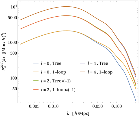
Figure 1: The invariant power spectra $P^{22;l}_{X}(k)$ of a rank-2 tensor field in a simple model. The predictions of the tree (lowest-order) approximation and those of one-loop approximation are plotted, while they are almost overlapped with each other. From bottom to top, the power spectra with $l=0,2,4$ are shown respectively. The power spectrum with $l=2$ is negative and is multiplied by $-1$ in the plot. The absolute values of spectra with one-loop approximations are slightly larger than those of tree approximations, depending on scales.

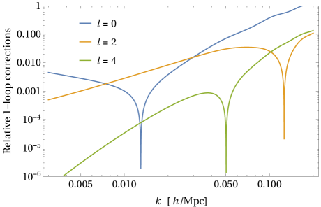
Figure 2: Absolute values of contributions to the power spectra of one-loop corrections relative to those of lowest-order approximations, $|P^{22;l}_{X}(k)/P^{22;l}_{X,\mathrm{L}}(k)-1|$.

In the following, we show the results of numerical calculations of the equations described above. The linear power spectrum $P_{\mathrm{L}}(k)$ of the mass density is calculated by a Boltzmann code CLASS [39, 40] with a flat $\Lambda$CDM model and cosmological parameters $h=0.6732$, $\Omega_{\mathrm{b}0}h^{2}=0.02238$, $\Omega_{\mathrm{cdm}}h^{2}=0.1201$, $n_{\mathrm{s}}=0.9660$, $\sigma_{8}=0.8120$ (Planck 2018 [2]). We apply a smoothing radius of $R=5\,h^{-1}\mathrm{Mpc}$ in the smoothing function of the biasing model. All the bias parameters are simply substituted by unity, $b^{(1)}_{X2}=b^{(2)}_{X2.00}=b^{(2)}_{X2;02}=b^{(2)}_{X2;20}=b^{(2)}_{X2;22}=1$, just for an illustrative purpose. The interchange symmetry of Eq. (94) requires an identity, $b^{(2)}_{X2;02}=b^{(2)}_{X2;20}$. For the fast Hankel transforms, we use a Mathematica version of the numerical code FFTLog [34]. One should note that the adopted values of the bias parameters in this example, especially higher-order ones, might be too large to be realistic in possible tensor fields, and nonlinear effects presented below could be larger than those in realistic situations.

The results of the power spectra of the rank-2 tensor field, $P^{22;l}_{X}(k)$, are shown in Fig. 1. The sign of the spectrum $P^{22;2}_{X}(k)$ is negative. The predictions of the lowest-order approximation, $P^{22;l}_{X\,[1]}(k)$ are simultaneously shown in the plot as indicated by “Tree” in the legends, together with the result including one-loop corrections as indicated by “1-loop” in the legends. One immediately notices that the effects of 1-loop corrections are small on large scales for all cases. In the case of $l=0$, the one-loop corrections significantly appear on smaller scales. However, this significance is partly due to our choice of relatively large values of higher-order bias parameters.

In Fig. 2, absolute values of relative fractions of the one-loop corrections to the lowest-order approximations, $|P^{22;l}_{X}(k)/P^{22;l}_{X,\mathrm{L}}(k)-1|$, are plotted, where $P^{22;l}_{X,\mathrm{L}}(k)$ is the lowest-order prediction without loop corrections. Overall, the larger the scales are (the smaller the wavenumbers are), the smaller the effects of one-loop corrections are. In the case of $l=0$, however, there remains a constant contribution of the one-loop correction in the power spectrum, which is manifested in Fig. 2 that the difference from the linear theory is increasing toward $k\rightarrow 0$ limit. In other cases of $l=2,4$, this kind of shot noise-like contribution does not exist, because of the asymptotic behavior of the spherical Bessel function $j_{l}(z)\rightarrow 0$ when $z\rightarrow 0$ for $l\geq 1$. The shot noise-like contribution in the one-loop power spectrum is already known to exist also in the scalar perturbation theory, and a hint of this effect is really seen in $N$-body simulations [26, 41]. However, as shown below, this constant contribution of the one-loop contributions does not contribute to the correlation function at a finite separation, because a constant in the power spectrum corresponds to the delta function at the origin in the correlation function. One should note that the small scales of $k\gtrsim 0.1\,h\,\mathrm{Mpc}^{-1}$ do not have physical significance in the current situation, because they are smaller than the smoothing radius $R=5\,h^{-1}\mathrm{Mpc}$ in this example. Therefore, the lowest-order approximation of the rank-2 tensor fields with multipoles of $l=2,4$ is already accurate without loop corrections, provided that our simplified assumption holds that they are biased from only second derivatives of the linear gravitational potential in the present model.

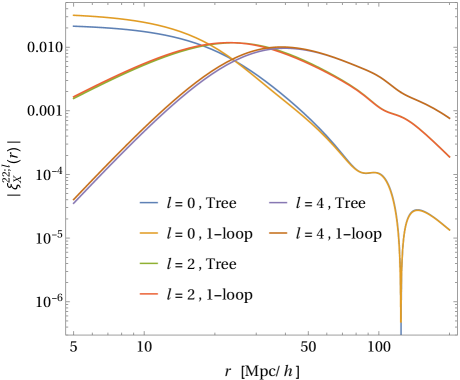
Figure 3: The invariant correlation functions $\xi^{22;l}_{X}(r)$ of a rank-2 tensor field in a simple model. The predictions of tree (lowest-order) approximation and those of one-loop approximation for $l=0,2,4$ are plotted. The colors of lines correspond to those in Fig. 1. The absolute values of correlation functions with the one-loop approximation are larger than those of tree approximation on small scales, $r\lesssim 20\,h^{-1}\mathrm{Mpc}$. On scales of less than $100\,h^{-1}\mathrm{Mpc}$, the signs of the correlation functions are $\xi^{22;0}_{X}>0$, $\xi^{22;2}_{X}<0$ and $\xi^{22;4}_{X}>0$ in this example. The sign for $l=0$ changes beyond the BAO scale of $\sim 105\,h^{-1}\mathrm{Mpc}$.

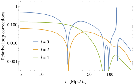
Figure 4: Contributions to the correlation functions of one-loop corrections relative to those of lowest-order approximations, $|\xi^{22;l}_{X}(r)/\xi^{22;l}_{X,\mathrm{L}}(r)-1|$.

We next calculate the correlation function of the rank-2 tensor field $\xi^{22;l}_{X}(r)$. The invariant correlation function of the tensor field is given by a Hankel transform of the invariant power spectrum by Eq. (69), which is again readily calculated by FFTLog. The results are plotted in Fig. 3. The absolute values of the relative fraction of the loop corrections, $|\xi^{22;l}_{X}(r)/\xi^{22;l}_{X,\mathrm{L}}(r)-1|$, are plotted in Fig. 4, where $\xi^{22;l}_{X,\mathrm{L}}(r)$ is the lowest-order prediction without loop corrections. As seen in both figures, the loop corrections to the correlation functions are not negligible on scales of $r\lesssim 50\,h^{-1}\mathrm{Mpc}$ at the level of 10% order. On large scales of $r\gtrsim 50\,h^{-1}\mathrm{Mpc}$, including the scales of BAO, the lowest-order approximations without loop corrections are fairly accurate roughly at the level of 1% order or less, with an exception near the scales of BAO, $\sim 100\,h^{-1}\mathrm{Mpc}$ in the case of monopole component $l=0$, which crosses the zero value near there. However, the fairly large contributions of nonlinear effects might be again due to our choice of large bias parameters.

In the above, we just exemplify applications of the formalism developed in this paper to calculate loop corrections of the power spectrum and correlation function, with a simple model that the tensor bias is given only by second-order derivatives of the linear potential of the gravitational field in Lagrangian space. We do not pursue further interpretations of these particular results in detail, which is beyond the scope of this paper. Some generalizations of the models of shape bias, and detailed analyses of the particular predictions of the rank-2 tensors in relation to the intrinsic alignment of galaxies will be addressed in future work [42].

V Conclusions

In this paper, we explicitly derive one-loop approximations of the power spectrum and correlation function of tensor fields, using the basic formulation developed in Paper I. The theory is built upon the formalism of iPT and its generalization to include arbitrarily biased tensor fields. As an example of applications, we explicitly and numerically evaluate the one-loop power spectrum and correlation function of the rank-2 tensor field with a model that the bias of the tensor field is given by a function of second-order derivatives of the gravitational potential. Higher-loop corrections are similarly possible to calculate along the line of this paper. Formal expressions of the all-order power spectrum are also obtained.

The original formalism of iPT is constructed in terms of Cartesian wavevectors which appear in the functions of renormalized bias functions and propagators. Since the tensor fields are decomposed into spherical tensors in the present formalism, the functions which involve wavevectors are naturally decomposed also into the spherical basis. The renormalized bias functions and propagators are decomposed into polypolar spherical harmonics in general. Unlike the previous methods of the perturbation theory with spherical tensors, the coordinates system of the spherical basis is not fixed to the direction of a wavevector of perturbation mode, and the fully rotational covariance is explicitly kept in the theory.

We define the rotationally invariant power spectrum and correlation function of the tensor field on a spherical basis. As our formalism uses the invariant functions for renormalized bias functions and propagators, the invariant power spectrum and correlation functions are also naturally represented by the invariant functions in loop corrections. This is one of the benefits of the fully rotational covariance of the theory in our formalism.

The redshift space distortions are also naturally incorporated into formalism. Due to the rotational covariance of the theory, the line of sight can be in arbitrary directions. The renormalized bias functions and propagators have additional dependence on the direction of the line of sight, which is also expanded by polypolar spherical harmonics together with the direction of wavevectors. The resulting propagators represented on a spherical basis are also rotationally invariant. This is in contrast to the common treatment of the redshift space distortions in perturbation theory, in which the direction of the line of sight is fixed to, e.g., the third axis of the coordinates system.

It has been known that the multi-dimensional integrations in the loop corrections can reduce to a series of one-dimensional Hankel transforms by spherical decomposition of the wavevectors in the kernel functions of the nonlinear perturbation theory and all the necessary integrals can be evaluated by an algorithm of FFTLog. The present formalism is also based on spherical decomposition of tensor field, essentially the same properties are naturally derived. In fact, when we consider the simplest case of a rank-0 tensor without bias, the previously known formula of the perturbation theory using the FFT algorithm is exactly reproduced. In the presence of (semi-)local models of bias, the same technique can be applied and all multi-dimensional integrations in the one-loop corrections reduce to a series of one-dimensional Hankel transforms, and thus are numerically calculated in very short time using FFTLog. In our rotationally covariant formalism with the redshift space distortions, the stunning property of reducing the dimensionality of integrals still holds even in redshift space.

In the last section, a simple example of the one-loop corrections of the power spectrum and correlation function of the rank-2 tensor field is presented and the results are numerically evaluated. In this example, we assume the rank-2 tensor field is biased from the second-order spatial derivatives of the gravitational potential. The numerical integrations with FFTLog are quite stable and fast enough. This example of tensor bias corresponds to the intrinsic alignment driven by the mass density field and gravitational shear or tidal field. Comparing these results with catalogs of halo shapes in numerical simulations should be a straightforward and interesting application of the present calculations.

More complicated modeling of the tensor bias, such as partial inclusions of the property of the halo model, can be an interesting application. Due to the generality of the present formalism, any model of the tensor bias can be taken into account, as long as the renormalized bias functions can be calculated. The bias model can even be a singular function of the density field, as in the case of the halo model [43, 27, 44]. This is in contrast to other methods in which the bias function is expanded in the Taylor series, and thus fully nonlinear or singular functions in the bias relation, such as halo bias cannot be taken into account. Investigations along this line are now under progress and will be presented in future work [42]. In realistic observations, most likely we can observe only projected tensors on the two-dimensional sky, rather than three-dimensional tensors themselves. It is technically straightforward to transform our results of the power spectrum and correlation function into projected tensors [24]. Characterizing galaxy shapes by higher-rank tensors can also be an interesting direction of research [45]. We will address the issue of projection effects in Paper III [46].

Appendix A Formal expressions of the nonlinear power spectrum to all orders

In the main text, we derive the full expressions of the one-loop power spectra in real space and redshift space. Higher-loop corrections can be calculated in the same way. The calculations of the higher-order propagators with loop corrections are involved and tedious. However, assuming the propagators are given, the expressions of the higher-loop corrections, which generalize Eqs. (83) and (85), can be formally derived to all orders. The derivation is simply a generalization of the derivation of Eqs. (83) and (85). In this Appendix, the derivation is illustrated and the resulting expressions are explicitly given.

We assume the Gaussian initial condition. The formal expression of the power spectrum to all orders is formally given by straightforward generalization of Ref. [26] for scalar fields to tensor fields,

$$P^{(l_{1}l_{2})}_{X_{1}X_{2}m_{1}m_{2}}(\bm{k})=\Pi^{2}(\bm{k})\sum_{n=1}^{\infty}\frac{1}{n!}\int\frac{d^{3}k^{(1)}}{(2\pi)^{3}}\cdots\frac{d^{3}k^{(n)}}{(2\pi)^{3}}(2\pi)^{3}\delta_{\mathrm{D}}^{3}(\bm{k}^{(1)}+\cdots+\bm{k}^{(n)}-\bm{k})\\ \times\hat{\Gamma}^{(n)}_{X_{1}l_{1}m_{1}}(\bm{k}^{(1)},\ldots,\bm{k}^{(n)})\hat{\Gamma}^{(n)}_{X_{2}l_{2}m_{2}}(-\bm{k}^{(1)},\ldots,-\bm{k}^{(n)})P_{\mathrm{L}}(k^{(1)})\cdots P_{\mathrm{L}}(k^{(n)}).$$ (127)

The expression of Eq. (127) holds both in real space and in redshift space. In redshift space, the power spectrum and propagators depend also on the direction of the line of sight, $\hat{\bm{z}}$.

A.0.1 Real space

We first consider the power spectrum in real space. As shown in Paper I, the directional dependence of $n$th-order normalized propagator on wavevectors is expanded by the polypolar spherical harmonics as

$$\hat{\Gamma}^{(n)}_{Xlm}(\bm{k}^{(1)},\cdots,\bm{k}^{(n)})=\sum_{\begin{subarray}{c}l^{(1)},\ldots,l^{(n)}\\ L^{(2)},\ldots,L^{(n-1)}\end{subarray}}\hat{\Gamma}^{(n)\,l;L^{(2)}\cdots L^{(n-1)}}_{Xl^{(1)}\cdots l^{(n)}}(k^{(1)},\cdots,k^{(n)})X^{l^{(1)}\cdots l^{(n)}}_{L^{(1)}\cdots L^{(n-1)};lm}(\hat{\bm{k}}^{(1)},\cdots,\hat{\bm{k}}^{(n)})$$ (128)

The polypolar spherical harmonics of order $n$ are introduced in Paper I, and their definitions are

$$X^{l_{1}l_{2}\cdots l_{n}}_{L_{2}L_{3}\cdots L_{n-1};lm}(\bm{n}_{1},\bm{n}_{2},\ldots,\bm{n}_{n})=(-1)^{L_{2}+\cdots+L_{n-1}}\sqrt{\{L_{2}\}\{L_{3}\}\cdots\{L_{n-1}\}}\left(l\,l_{1}\,L_{2}\right)_{m}^{\phantom{m}m_{1}M_{2}}\left(L_{2}\,l_{2}\,L_{3}\right)_{M_{2}}^{\phantom{M_{2}}m_{2}M_{3}}\cdots\left(L_{n-2}\,l_{n-2}\,L_{n-1}\right)_{M_{n-2}}^{\phantom{M_{n-2}}m_{n-2}M_{n-1}}\\ \times\left(L_{n-1}\,l_{n-1}\,l_{n}\right)_{M_{n-1}}^{\phantom{M_{n-1}}m_{n-1}m_{n}}C_{l_{1}m_{1}}(\bm{n}_{1})C_{l_{2}m_{2}}(\bm{n}_{2})\cdots C_{l_{n}m_{n}}(\bm{n}_{n}),$$ (129)

where $C_{lm}(\bm{n})$ are the spherical harmonics with Racah’s normalization defined in the main text by Eq. (3), and $(l_{1}\,l_{2}\,l_{3})_{m_{1}}^{\phantom{m_{1}}m_{2}m_{3}}$ is our notation of the $3j$-symbol in the main text by Eq. (6). As in the main text, we use a simplified notation for factors $\{L\}\equiv 2L+1$, $\{l\}\equiv 2l+1$, and so forth. The polypolar spherical harmonics are straightforward generalization of the bipolar and tripolar spherical harmonics, defined in the main text by Eqs. (5) and (20), respectively.

Substituting Eq. (128) into Eq. (127), a product of two polypolar spherical harmonics appears. This product reduces to a single polypolar spherical harmonics as (Paper I)

$$X^{l_{1}l_{2}\cdots l_{n}}_{L_{2}L_{3}\cdots L_{n-1};lm}(\bm{n}_{1},\bm{n}_{2},\ldots,\bm{n}_{n})X^{l_{1}^{\prime}l_{2}^{\prime}\cdots l_{n}^{\prime}}_{L_{2}^{\prime}L_{3}^{\prime}\cdots L_{n-1}^{\prime};l^{\prime}m^{\prime}}(\bm{n}_{1},\bm{n}_{2},\ldots,\bm{n}_{n})=\sqrt{\{L_{2}\}\cdots\{L_{n-1}\}\{L_{2}^{\prime}\}\cdots\{L_{n-1}^{\prime}\}}\sum_{l^{\prime\prime}}(-1)^{l^{\prime\prime}}\{l^{\prime\prime}\}\left(l\,l^{\prime}\,l^{\prime\prime}\right)_{mm^{\prime}}^{\phantom{mm^{\prime}}m^{\prime\prime}}\\ \times\sum_{l_{1}^{\prime\prime},\ldots,l_{n}^{\prime\prime}}(-1)^{l_{1}^{\prime\prime}+\cdots+l_{n}^{\prime\prime}}\{l_{1}^{\prime\prime}\}\cdots\{l_{n}^{\prime\prime}\}\begin{pmatrix}l_{1}&l_{1}^{\prime}&l_{1}^{\prime\prime}\\ 0&0&0\end{pmatrix}\cdots\begin{pmatrix}l_{n}&l_{n}^{\prime}&l_{n}^{\prime\prime}\\ 0&0&0\end{pmatrix}\sum_{L_{2}^{\prime\prime},\ldots,L_{n-1}^{\prime\prime}}\sqrt{\{L_{2}^{\prime\prime}\}\cdots\{L_{n-1}^{\prime\prime}\}}\begin{Bmatrix}l&l^{\prime}&l^{\prime\prime}\\ l_{1}&l_{1}^{\prime}&l_{1}^{\prime\prime}\\ L_{2}&L_{2}^{\prime}&L_{2}^{\prime\prime}\end{Bmatrix}\\ \times\begin{Bmatrix}L_{2}&L_{2}^{\prime}&L_{2}^{\prime\prime}\\ l_{2}&l_{2}^{\prime}&l_{2}^{\prime\prime}\\ L_{3}&L_{3}^{\prime}&L_{3}^{\prime\prime}\end{Bmatrix}\cdots\begin{Bmatrix}L_{n-2}&L_{n-2}^{\prime}&L_{n-2}^{\prime\prime}\\ l_{n-2}&l_{n-2}^{\prime}&l_{n-2}^{\prime\prime}\\ L_{n-1}&L_{n-1}^{\prime}&L_{n-1}^{\prime\prime}\end{Bmatrix}\begin{Bmatrix}L_{n-1}&L_{n-1}^{\prime}&L_{n-1}^{\prime\prime}\\ l_{n-1}&l_{n-1}^{\prime}&l_{n-1}^{\prime\prime}\\ l_{n}&l_{n}^{\prime}&l_{n}^{\prime\prime}\end{Bmatrix}X^{l_{1}^{\prime\prime}l_{2}^{\prime\prime}\cdots l_{n}^{\prime\prime}}_{L_{2}^{\prime\prime}L_{3}^{\prime\prime}\cdots L_{n-1}^{\prime\prime};l^{\prime\prime}m^{\prime\prime}}(\bm{n}_{1},\bm{n}_{2},\ldots,\bm{n}_{n}).$$ (130)

The integrals with a delta function in Eq. (127) is substituted by

$$\int\frac{d^{3}k^{(1)}}{(2\pi)^{3}}\cdots\frac{d^{3}k^{(n)}}{(2\pi)^{3}}(2\pi)^{3}\delta_{\mathrm{D}}^{3}(\bm{k}^{(1)}+\cdots+\bm{k}^{(n)}-\bm{k})\times\cdots=\int d^{3}r\,e^{-i\bm{k}\cdot\bm{r}}\int\frac{d^{3}k^{(1)}}{(2\pi)^{3}}\cdots\frac{d^{3}k^{(n)}}{(2\pi)^{3}}e^{i(\bm{k}^{(1)}+\cdots+\bm{k}^{(n)})\cdot\bm{r}}\times\cdots.$$ (131)

Angular components of the wavevectors $\bm{k}^{(1)},\ldots,\bm{k}^{(n)}$ in the integrand of Eq. (127) only appear in the polypolar spherical harmonics. Consecutively using Eqs. (13), (58), (42) and (45), one can show that the necessary integrals are given by

$$\int\frac{d^{2}\hat{k}^{(1)}}{4\pi}\cdots\frac{d^{2}\hat{k}^{(n)}}{4\pi}e^{i(\bm{k}^{(1)}+\cdots+\bm{k}^{(n)})\cdot\bm{r}}X^{l_{1}l_{2}\cdots l_{n}}_{L_{2}L_{3}\cdots L_{n-1};lm}\left(\bm{k}^{(1)},\bm{k}^{(2)},\ldots,\bm{k}^{(n)}\right)=\frac{(-1)^{l}{\{l\}}}{(4\pi)^{n}}(-i)^{l_{1}+\cdots+l_{n}}(-1)^{L_{2}+\cdots+L_{n-1}}\{l_{1}\}\cdots\{l_{n}\}\\ \times j_{l_{1}}\left(k^{(1)}r\right)\cdots j_{l_{n}}\left(k^{(n)}r\right)\sqrt{\{L_{2}\}\cdots\{L_{n-1}\}}\begin{pmatrix}l&l_{1}&L_{2}\\ 0&0&0\end{pmatrix}\begin{pmatrix}L_{2}&l_{2}&L_{3}\\ 0&0&0\end{pmatrix}\cdots\begin{pmatrix}L_{n-2}&l_{n-2}&L_{n-1}\\ 0&0&0\end{pmatrix}\begin{pmatrix}L_{n-1}&l_{n-1}&l_{n}\\ 0&0&0\end{pmatrix}C_{lm}(\bm{r}).$$ (132)

Putting the above equations together, the angular integrations in Eq. (127) is analytically evaluated. Comparing the result with Eq. (57), or directly using Eq. (59), we finally derive the invariant power spectrum to all orders in real space as

$$P^{l_{1}l_{2};l}_{X_{1}X_{2}}(k)=(-1)^{l}\{l\}\,\Pi^{2}(k)\,4\pi\int r^{2}dr\,j_{l}(kr)\sum_{n=1}^{\infty}\frac{1}{n!}\sum_{\begin{subarray}{c}l^{(1)},\ldots,l^{(n)},L^{(2)},\ldots,L^{(n-1)}\\ l_{1}^{(1)},\ldots,l_{1}^{(n)},L_{1}^{(2)},\ldots,L_{1}^{(n-1)}\\ l_{2}^{(1)},\ldots,l_{2}^{(n)},L_{2}^{(2)},\ldots,L_{2}^{(n-1)}\end{subarray}}i^{l+l^{(1)}+\cdots+l^{(n)}}(-1)^{l_{2}^{(1)}+\cdots+l_{2}^{(n)}}(-1)^{L^{(2)}+\cdots+L^{(n-1)}}\left\{l^{(1)}\right\}\cdots\left\{l^{(n)}\right\}\\ \times\left\{L^{(2)}\right\}\cdots\left\{L^{(n-1)}\right\}\sqrt{\left\{L_{1}^{(2)}\right\}\cdots\left\{L_{1}^{(n-1)}\right\}\left\{L_{1}^{(2)}\right\}\cdots\left\{L_{1}^{(n-1)}\right\}}\begin{pmatrix}l_{1}^{(1)}&l_{2}^{(1)}&l^{(1)}\\ 0&0&0\end{pmatrix}\cdots\begin{pmatrix}l_{1}^{(n)}&l_{2}^{(n)}&l^{(n)}\\ 0&0&0\end{pmatrix}\begin{pmatrix}l&l^{(1)}&L^{(2)}\\ 0&0&0\end{pmatrix}\\ \times\begin{pmatrix}L^{(2)}&l^{(2)}&L^{(3)}\\ 0&0&0\end{pmatrix}\cdots\begin{pmatrix}L^{(n-2)}&l^{(n-2)}&L^{(n-1)}\\ 0&0&0\end{pmatrix}\begin{pmatrix}L^{(n-1)}&l^{(n-1)}&l^{(n)}\\ 0&0&0\end{pmatrix}\begin{Bmatrix}l_{1}&l_{2}&l\\ l_{1}^{(1)}&l_{2}^{(1)}&l^{(1)}\\ L_{1}^{(2)}&L_{2}^{(2)}&L^{(2)}\end{Bmatrix}\\ \times\begin{Bmatrix}L_{1}^{(2)}&L_{2}^{(2)}&L^{(2)}\\ l_{1}^{(2)}&l_{2}^{(2)}&l^{(2)}\\ L_{1}^{(3)}&L_{2}^{(3)}&L^{(3)}\end{Bmatrix}\cdots\begin{Bmatrix}L_{1}^{(n-2)}&L_{2}^{(n-2)}&L^{(n-2)}\\ l_{1}^{(n-2)}&l_{2}^{(n-2)}&l^{(n-2)}\\ L_{1}^{(n-1)}&L_{2}^{(n-1)}&L^{(n-1)}\end{Bmatrix}\begin{Bmatrix}L_{1}^{(n-1)}&L_{2}^{(n-1)}&L^{(n-1)}\\ l_{1}^{(n-1)}&l_{2}^{(n-1)}&l^{(n-1)}\\ l_{1}^{(n)}&l_{2}^{(n)}&l^{(n)}\end{Bmatrix}\int\frac{{k^{(1)}}^{2}dk^{(1)}}{2\pi^{2}}\cdots\frac{{k^{(n)}}^{2}dk^{(n)}}{2\pi^{2}}P_{\mathrm{L}}\left(k^{(1)}\right)\cdots P_{\mathrm{L}}\left(k^{(n)}\right)\\ \times j_{l^{(1)}}\left(k^{(1)}r\right)\cdots j_{l^{(n)}}\left(k^{(n)}r\right)\ \hat{\Gamma}^{(n)\,l_{1};L_{1}^{(2)}\cdots L_{1}^{(n-1)}}_{X_{1}l_{1}^{(1)}\cdots l_{1}^{(n)}}\left(k^{(1)},\ldots,k^{(n)}\right)\hat{\Gamma}^{(n)\,l_{2};L_{2}^{(2)}\cdots L_{2}^{(n-1)}}_{X_{2}l_{2}^{(1)}\cdots l_{2}^{(n)}}\left(k^{(1)},\ldots,k^{(n)}\right).$$ (133)

If the propagators in the spherical basis of the last two factors are given by the sum of terms in which the dependencies on the $k^{(1)},\ldots,k^{(n)}$ are separated, the above integrals are calculated by a series of one-dimensional Hankel transforms using FFTLog. For the gravitational evolution part, that is really the case in the one-loop order as we explicitly show in the main text, and also in the two-loop order [35]. For the bias part, it is the case for the semi-local models as we see in the main text.

A.0.2 Redshift space

A formal expression to all orders of the power spectrum in redshift space can also be derived similarly as in the above case for real space. The derivation is a straightforward generalization of the one-loop expression given in Eq. (85). All the necessary equations are given in above. We have extra dependence of the propagators on the line-of-sight direction $\hat{\bm{z}}$. The $n$th-order normalized propagator is expanded as (Paper I)

$$\hat{\Gamma}^{(n)}_{Xlm}(\bm{k}_{1},\cdots,\bm{k}_{n};\hat{\bm{z}};k,\mu)=\sum_{\begin{subarray}{c}l_{z},l_{1},\ldots,l_{n}\\ L_{1},\ldots,L_{n-1}\end{subarray}}\hat{\Gamma}^{(n)\,l\,l_{z};L_{1}\cdots L_{n-1}}_{Xl_{1}\cdots l_{n}}(k_{1},\cdots,k_{n};k,\mu)X^{l_{z}l_{1}\cdots l_{n}}_{L_{1}\cdots L_{n-1};lm}(\hat{\bm{z}},\hat{\bm{k}}_{1},\cdots,\hat{\bm{k}}_{n}).$$ (134)

This expansion is substituted in Eq. (127), and follow the rest of calculations in the case of real space above. The consequent result is compared with Eq. (62), or directly substituted into Eq. (63), we finally derive the invariant power spectrum to all orders in redshift space as

$$P^{l_{1}l_{2};l\,l_{z};L}_{X_{1}X_{2}}(k,\mu)=(-)^{l+l_{z}}\{l\}\{l_{z}\}\sqrt{\{L\}}\,\Pi^{2}(k,\mu)\,4\pi\int r^{2}dr\,j_{l}(kr)\sum_{n=1}^{\infty}\frac{1}{n!}\sum_{\begin{subarray}{c}l^{(1)},\ldots,l^{(n)},L^{(2)},\ldots,L^{(n-1)}\\ l_{1}^{(1)},\ldots,l_{1}^{(n)},L_{1}^{(2)},\ldots,L_{1}^{(n-1)}\\ l_{2}^{(1)},\ldots,l_{2}^{(n)},L_{2}^{(2)},\ldots,L_{2}^{(n-1)}\end{subarray}}i^{l+l^{(1)}+\cdots+l^{(n)}}(-1)^{l_{2}^{(1)}+\cdots+l_{2}^{(n)}}(-1)^{L^{(2)}+\cdots+L^{(n-1)}}\\ \times\left\{l^{(1)}\right\}\cdots\left\{l^{(n)}\right\}\left\{L^{(2)}\right\}\cdots\left\{L^{(n-1)}\right\}\sqrt{\left\{L_{1}^{(2)}\right\}\cdots\left\{L_{1}^{(n-1)}\right\}\left\{L_{1}^{(2)}\right\}\cdots\left\{L_{1}^{(n-1)}\right\}}\begin{pmatrix}l_{1}^{(1)}&l_{2}^{(1)}&l^{(1)}\\ 0&0&0\end{pmatrix}\cdots\begin{pmatrix}l_{1}^{(n)}&l_{2}^{(n)}&l^{(n)}\\ 0&0&0\end{pmatrix}\begin{pmatrix}l&l^{(1)}&L^{(2)}\\ 0&0&0\end{pmatrix}\\ \times\begin{pmatrix}L^{(2)}&l^{(2)}&L^{(3)}\\ 0&0&0\end{pmatrix}\cdots\begin{pmatrix}L^{(n-2)}&l^{(n-2)}&L^{(n-1)}\\ 0&0&0\end{pmatrix}\begin{pmatrix}L^{(n-1)}&l^{(n-1)}&l^{(n)}\\ 0&0&0\end{pmatrix}\sum_{l_{z1},l_{z2},L_{1},L_{2}}\sqrt{\left\{L_{1}\right\}\left\{L_{2}\right\}}\begin{pmatrix}l_{z1}&l_{z2}&l_{z}\\ 0&0&0\end{pmatrix}\begin{Bmatrix}l_{1}&l_{2}&L\\ l_{z1}&l_{z2}&l_{z}\\ L_{1}&L_{2}&l\end{Bmatrix}\\ \times\begin{Bmatrix}L_{1}&L_{2}&l\\ l_{1}^{(1)}&l_{2}^{(1)}&l^{(1)}\\ L_{1}^{(2)}&L_{2}^{(2)}&L^{(2)}\end{Bmatrix}\begin{Bmatrix}L_{1}^{(2)}&L_{2}^{(2)}&L^{(2)}\\ l_{1}^{(2)}&l_{2}^{(2)}&l^{(2)}\\ L_{1}^{(3)}&L_{2}^{(3)}&L^{(3)}\end{Bmatrix}\cdots\begin{Bmatrix}L_{1}^{(n-2)}&L_{2}^{(n-2)}&L^{(n-2)}\\ l_{1}^{(n-2)}&l_{2}^{(n-2)}&l^{(n-2)}\\ L_{1}^{(n-1)}&L_{2}^{(n-1)}&L^{(n-1)}\end{Bmatrix}\begin{Bmatrix}L_{1}^{(n-1)}&L_{2}^{(n-1)}&L^{(n-1)}\\ l_{1}^{(n-1)}&l_{2}^{(n-1)}&l^{(n-1)}\\ l_{1}^{(n)}&l_{2}^{(n)}&l^{(n)}\end{Bmatrix}\\ \times\int\frac{{k^{(1)}}^{2}dk^{(1)}}{2\pi^{2}}\cdots\frac{{k^{(n)}}^{2}dk^{(n)}}{2\pi^{2}}P_{\mathrm{L}}\left(k^{(1)}\right)\cdots P_{\mathrm{L}}\left(k^{(n)}\right)j_{l^{(1)}}\left(k^{(1)}r\right)\cdots j_{l^{(n)}}\left(k^{(n)}r\right)\ \\ \times\hat{\Gamma}^{(n)\,l_{1}l_{z1};L_{1}L_{1}^{(2)}\cdots L_{1}^{(n-1)}}_{X_{1}l_{1}^{(1)}\cdots l_{1}^{(n)}}\left(k^{(1)},\ldots,k^{(n)};k,\mu\right)\hat{\Gamma}^{(n)\,l_{2}l_{z2};L_{2}L_{2}^{(2)}\cdots L_{2}^{(n-1)}}_{X_{2}l_{2}^{(1)}\cdots l_{2}^{(n)}}\left(k^{(1)},\ldots,k^{(n)};k,\mu\right).$$ (135)

As a consistency check, we readily see that this expression exactly reduces to Eq. (133) when we substitute $l_{z}=l_{z1}=l_{z2}=0$, using Eq. (79). In the case of semi-local models of bias, the radial integrals are calculated by a series of one-dimensional Hankel transforms using FFTLog, just as in the case of real space.

References

- [1] T. Matsubara, [arXiv:2210.10435] (Paper I)
- [2] N. Aghanim et al. [Planck], Astron. Astrophys. 641, A6 (2020) [erratum: Astron. Astrophys. 652, C4 (2021)]
- [3] C. D. Rimes and A. J. S. Hamilton, Mon. Not. Roy. Astron. Soc. 360, L82-L86 (2005)
- [4] F. Bernardeau, M. Crocce and R. Scoccimarro, Phys. Rev. D 78, 103521 (2008)
- [5] D. J. Eisenstein et al. [SDSS], Astrophys. J. 633, 560-574 (2005)
- [6] R. Juszkiewicz, Mon. Not. R. Astron. Soc. 197, 931 (1981)
- [7] E. T. Vishniac, Mon. Not. R. Astron. Soc. 203, 345 (1983)
- [8] J. N. Fry, Astrophys. J. 279, 499-510 (1984)
- [9] M. H. Goroff, B. Grinstein, S. J. Rey and M. B. Wise, Astrophys. J. 311, 6-14 (1986)
- [10] Y. Suto and M. Sasaki, Phys. Rev. Lett. 66, 264-267 (1991)
- [11] N. Makino, M. Sasaki and Y. Suto, Phys. Rev. D 46, 585-602 (1992)
- [12] B. Jain and E. Bertschinger, Astrophys. J. 431, 495 (1994)
- [13] D. Jeong and E. Komatsu, Astrophys. J. 651, 619-626 (2006)
- [14] V. Desjacques, D. Jeong and F. Schmidt, Phys. Rept. 733, 1-193 (2018)
- [15] P. Catelan, M. Kamionkowski and R. D. Blandford, Mon. Not. Roy. Astron. Soc. 320, L7-L13 (2001)
- [16] T. Okumura and Y. P. Jing, Astrophys. J. Lett. 694, L83-L86 (2009)
- [17] B. Joachimi, M. Cacciato, T. D. Kitching, A. Leonard, R. Mandelbaum, B. M. Schäfer, C. Sifón, H. Hoekstra, A. Kiessling and D. Kirk, et al. Space Sci. Rev. 193, no.1-4, 1-65 (2015)
- [18] K. Kogai, T. Matsubara, A. J. Nishizawa and Y. Urakawa, JCAP 08, 014 (2018)
- [19] N. E. Chisari and C. Dvorkin, JCAP 12, 029 (2013)
- [20] J. Blazek, Z. Vlah and U. Seljak, JCAP 08, 015 (2015)
- [21] J. Blazek, N. MacCrann, M. A. Troxel and X. Fang, Phys. Rev. D 100, no.10, 103506 (2019)
- [22] D. M. Schmitz, C. M. Hirata, J. Blazek and E. Krause, JCAP 07, 030 (2018)
- [23] Z. Vlah, N. E. Chisari and F. Schmidt, JCAP 01, 025 (2020)
- [24] Z. Vlah, N. E. Chisari and F. Schmidt, JCAP 05, 061 (2021)
- [25] V. Desjacques, M. Crocce, R. Scoccimarro and R. K. Sheth, Phys. Rev. D 82, 103529 (2010)
- [26] T. Matsubara, Phys. Rev. D 83, 083518 (2011)
- [27] T. Matsubara, Phys. Rev. D 90, 043537 (2014)
- [28] M. Schmittfull, Z. Vlah and P. McDonald, Phys. Rev. D 93, no.10, 103528 (2016)
- [29] P. Catelan, Mon. Not. Roy. Astron. Soc. 276, 115 (1995)
- [30] P. Catelan and T. Theuns, Mon. Not. Roy. Astron. Soc. 282, 455 (1996)
- [31] T. Matsubara, Phys. Rev. D 92, no.2, 023534 (2015)
- [32] F. Bernardeau, S. Colombi, E. Gaztanaga and R. Scoccimarro, Phys. Rept. 367, 1-248 (2002)
- [33] T. Matsubara, Phys. Rev. D 77, 063530 (2008)
- [34] A. J. S. Hamilton, Mon. Not. Roy. Astron. Soc. 312, 257-284 (2000)
- [35] M. Schmittfull and Z. Vlah, Phys. Rev. D 94, no.10, 103530 (2016)
- [36] J. E. McEwen, X. Fang, C. M. Hirata and J. A. Blazek, JCAP 09, 015 (2016)
- [37] X. Fang, J. A. Blazek, J. E. McEwen and C. M. Hirata, JCAP 02, 030 (2017)
- [38] D. A. Varshalovich, A. N. Moskalev and V. K. Khersonskii, “Quantum Theory Of Angular Momentum,” (World Scientific Publishing, Singapore, 1988)
- [39] J. Lesgourgues, [arXiv:1104.2932 [astro-ph.IM]].
- [40] D. Blas, J. Lesgourgues and T. Tram, JCAP 07, 034 (2011)
- [41] M. Sato and T. Matsubara, Phys. Rev. D 84, 043501 (2011)
- [42] T. Matsubara, K. Akitsu and A. Taruya, in preparation.
- [43] T. Matsubara, Phys. Rev. D 86, 063518 (2012)
- [44] T. Matsubara and V. Desjacques, Phys. Rev. D 93, no.12, 123522 (2016)
- [45] K. Kogai, K. Akitsu, F. Schmidt and Y. Urakawa, JCAP 03, 060 (2021)
- [46] T. Matsubara, [arXiv:2304.13304] (Paper III)