Abstract

Expected precisions of measurements of the elastic scattering cross sections are estimated for $\mu^{+}\mu^{+}$ and $\mu^{+}e^{-}$ colliders, which are recently proposed as future realistic possibilities ($\mu$TRISTAN). Comparing with contributions from possible new physics represented by higher dimensional operators, we find that the measurements at a TeV energy $\mu^{+}\mu^{+}$ collider can probe the scale of new physics up to $O(100)$ TeV. A $\mu^{+}e^{-}$ collider for the Higgs boson factory can also improve the electroweak precision test.

1 Introduction

The technology of particle accelerations has made impressive progress since Van de Graaff and Cockcroft-Walton in the early 20th century. The energy frontier has now reached the center of mass energy of $O(10)$ TeV for hadron collisions, but still even higher energies are demanded from particle physics.

One of the important tasks in the future accelerator experiments will be to gather information of new physics that enables us to build a guidance for the big picture. In particular, at lepton colliders, well-defined initial states provide clean environment for the precision tests of scattering processes. Indeed, $e^{+}e^{-}$ colliders such as the LEP experiments at CERN have given important inputs towards the complete picture of the Standard Model [1, 2, 3]. In addition, the precision tests of the scattering processes have been giving severe constraints on the new physics contributions [4, 5, 6, 7, 8, 9, 10].

After the establishment of the Standard Model, at least of its particle content and its gauge group, one can now parametrize the effects of physics beyond the Standard Model as coefficients of higher dimensional operators in the Lagrangian of the Standard Model effective field theory (SMEFT) [11, 12, 13, 14]. Although there are possibilities of having light new particles, new physics models motivated by the UV origin of the Higgs boson can be generically fall into this type where new particles and/or new interactions appear at TeV or multi-TeV scale. Once a new lepton collider is to be built, the simplest and also one of the most important questions is how well such coefficients can be measured. At lepton colliders, there are enormous amount of elastic scattering events, which typically have a sharp peak in the forward region. The new physics effects interfere with the Standard-Model amplitude and modify the angular distribution mostly in the central region. Such anomalous distributions can be detected at a high accuracy and thus provides good probe of microscopic physics. Indeed, prospects at the ILC experiments have been studied, and significant improvement over the current limits has been reported [15, 16].

Recently, a new collider experiment, $\mu$TRISTAN [17], using the ultra-cold muon [18], has been proposed. The technology of $\mu^{+}$ cooling by the laser ionization of the muonium (the $\mu^{+}e^{-}$ bound state) has been developed for the muon $g-2$/EDM experiment at J-PARC [19]. This technology enables us to consider realistic $\mu^{+}e^{-}$ and $\mu^{+}\mu^{+}$ colliders. As a possible design for a 3 km storage ring, it has been considered to accelerate $\mu^{+}$ and $e^{-}$ beams up to 1 TeV and 30 GeV, respectively, with which the $\mu^{+}e^{-}$ and $\mu^{+}\mu^{+}$ colliders with the center-of-mass energy to be 346 GeV and 2 TeV can be realized. The luminosities are estimated to be at the level of $10^{33-34}$ cm^-2 s^-1, with which the $\mu^{+}e^{-}$ collider can be a good Higgs boson factory whereas direct new particle searches are possible at the high energy $\mu^{+}\mu^{+}$ collider.

In this paper, we examine how well $\mu$TRISTAN can measure the elastic $\mu^{+}e^{-}$ and $\mu^{+}\mu^{+}$ scattering processes. Since the contributions from, for example, four-fermion operators are larger for higher energies, the $\mu^{+}\mu^{+}$ collider at 2 TeV should give the most stringent constraints on the coefficients. We indeed find that the collider can probe the energy scale of $O(100)$ TeV. We include all the SMEFT dimension-six operators that contribute to the elastic scattering. We find that the $\mu^{+}e^{-}$ collider at 346 GeV can improve the constraints on the electroweak precision observables such as $S$ and $T$ parameters [20, 21].

This paper is organized as follows. In Sec. 2, we give a review on SMEFT and specify the operators that we consider. We give the expected constraints on SMEFT operators at a $\mu^{+}\mu^{+}$ collider (Sec. 3) and at an $e^{-}\mu^{+}$ collider (Sec. 4). We compare our result with the current constraints in Sec. 5. Sec. 6 is devoted to the summary. In App. A, we present kinematic formulas relevant to an $e^{-}\mu^{+}$ collider, whose beam energies are asymmetric.

2 SMEFT Lagrangian

In this section, we present necessary formulas to calculate scatterings $e^{-}\mu^{+}\to e^{-}\mu^{+}$ and $\mu^{+}\mu^{+}\to\mu^{+}\mu^{+}$ within SMEFT. This includes a review on the relations between $(\alpha,M_{Z},G_{F})$ and SMEFT Lagrangian parameters. We consider up to dimension-six operators adopting the basis of ref. [22]. All calculations in this paper are performed at the tree level.

2.1 Gauge fields

Let us first consider Lagrangian for the gauge fields. The following four higher dimensional operators

$$Q_{HW}=H^{\dagger}HW_{\mu\nu}^{I}W^{I\mu\nu}$$ (1)

$$Q_{HB}=H^{\dagger}HB_{\mu\nu}B^{\mu\nu}$$ (2)

$$Q_{HWB}=H^{\dagger}\tau^{I}HW^{I}_{\mu\nu}B^{\mu\nu}$$ (3)

$$Q_{HD}=(H^{\dagger}D_{\mu}H)^{*}(H^{\dagger}D_{\mu}H)$$ (4)

are involved. The Lagrangian is given by

$$\mathcal{L}_{\rm gauge} =-\frac{1}{4}B^{\mu\nu}B_{\mu\nu}-\frac{1}{4}W_{\mu\nu}^{I}W^{I\mu\nu}+D_{\mu}H^{\dagger}D^{\mu}H$$

$$\qquad{}+C_{HW}H^{\dagger}HW_{\mu\nu}^{I}W^{I\mu\nu}+C_{HB}H^{\dagger}HB_{\mu\nu}B^{\mu\nu}+C_{HWB}H^{\dagger}\tau^{I}HW^{I}_{\mu\nu}B^{\mu\nu}$$

$$\qquad+C_{HD}(H^{\dagger}D_{\mu}H)^{*}(H^{\dagger}D_{\mu}H)$$

$$=-\frac{1}{4}(1-2v^{2}C_{HB})B^{\mu\nu}B_{\mu\nu}-\frac{1}{4}(1-2v^{2}C_{HW})W_{\mu\nu}^{3}W^{3\mu\nu}-\frac{v^{2}}{2}C_{HWB}W_{\mu\nu}^{3}B^{\mu\nu}$$

$$\qquad{}+(W^{3}_{\mu},B_{\mu})M\begin{pmatrix}W^{3}_{\mu}\\ B_{\mu}\end{pmatrix}-\frac{1}{2}(1-2v^{2}C_{HW})W_{\mu\nu}^{+}W^{\mu\nu-}+\frac{g^{2}v^{2}}{4}W_{\mu}^{+}W^{\mu-}+\cdots.$$ (5)

Here we define the matrix $M$ by

$$M =\left(1+\frac{v^{2}}{2}C_{HD}\right)\begin{pmatrix}\frac{g^{2}v^{2}}{8}&-\frac{g{g^{\prime}}v^{2}}{8}\\ -\frac{g{g^{\prime}}v^{2}}{8}&\frac{{g^{\prime}}^{2}v^{2}}{8}\end{pmatrix},$$ (6)

and define $W^{+}=\frac{1}{\sqrt{2}}(W^{1}-iW^{2})$ and $W^{-}=\frac{1}{\sqrt{2}}(W^{1}+iW^{2})$. In the final equality, we show explicitly only the part where the Higgs VEV is substituted and quadratic part in the gauge fields. We use $D_{\mu}H=(\partial_{\mu}+i\frac{g}{2}\tau^{I}W^{I}_{\mu}+i\frac{{g^{\prime}}}{2}B_{\mu})H$ and $\langle H\rangle=\frac{1}{\sqrt{2}}\begin{pmatrix}0\\ v\end{pmatrix}$.

Let us consider $A_{\mu}$ and $Z_{\mu}$ part, i.e., $B_{\mu}$ and $W_{\mu}^{3}$ part. We can diagonalize the matrix $M$ by

$$\begin{pmatrix}W^{3}_{\mu}\\ B_{\mu}\end{pmatrix}=\begin{pmatrix}\cos{\theta_{W}}&\sin{\theta_{W}}\\ -\sin{\theta_{W}}&\cos{\theta_{W}}\end{pmatrix}\begin{pmatrix}Z_{\mu}\\ A_{\mu}\end{pmatrix},$$ (7)

where $\cos{\theta_{W}}=g/\sqrt{g^{2}+{g^{\prime}}^{2}}$ and $\sin{\theta_{W}}={g^{\prime}}/\sqrt{g^{2}+{g^{\prime}}^{2}}$. Note that $\theta_{W}$ differs from the SM value of the Weinberg angle. This is because $g$ and ${g^{\prime}}$ are different from their SM values, which are determined by assuming the SM. The mass term turns into

$$(W^{3}_{\mu},B_{\mu})M\begin{pmatrix}W^{3}_{\mu}\\ B_{\mu}\end{pmatrix}=\frac{1}{2}(1+\frac{v^{2}}{2}C_{HD})\frac{1}{4}(g^{2}+{g^{\prime}}^{2})v^{2}Z_{\mu}Z^{\mu}.$$ (8)

Then the kinetic terms are written in the form of

$$\mathcal{L}=-\frac{1}{4}(1+\epsilon_{1})F_{\mu\nu}F^{\mu\nu}-\frac{1}{4}(1+\epsilon_{2})Z_{\mu\nu}Z^{\mu\nu}+\epsilon_{3}F_{\mu\nu}Z^{\mu\nu}.$$ (9)

Here the $\epsilon_{i}$ parameters are given by

$$\epsilon_{1}=-2v^{2}C_{HB}\cos^{2}{\theta_{W}}-2v^{2}C_{HW}\sin^{2}{\theta_{W}}+2v^{2}C_{HWB}\cos{\theta_{W}}\sin{\theta_{W}},$$ (10)

$$\epsilon_{2}=-2v^{2}C_{HB}\sin^{2}{\theta_{W}}-2v^{2}C_{HW}\cos^{2}{\theta_{W}}-2v^{2}C_{HWB}\cos{\theta_{W}}\sin{\theta_{W}},$$ (11)

$$\epsilon_{3}=-v^{2}C_{HB}\cos{\theta_{W}}\sin{\theta_{W}}+v^{2}C_{HW}\cos{\theta_{W}}\sin{\theta_{W}}-\frac{v^{2}}{2}C_{HWB}(\cos^{2}{\theta_{W}}-\sin^{2}{\theta_{W}}).$$ (12)

After the following (non-orthogonal) transformation

$$\begin{cases}A_{\mu}\to A_{\mu}+2\epsilon_{3}Z_{\mu}\\ Z_{\mu}\to Z_{\mu}\end{cases},$$ (13)

the kinetic term becomes

$$\mathcal{L}=-\frac{1}{4}(1+\epsilon_{1})F_{\mu\nu}F^{\mu\nu}-\frac{1}{4}(1+\epsilon_{2})Z_{\mu\nu}Z^{\mu\nu},$$ (14)

where the kinetic mixing is eliminated. Note that the mass term is invariant under the above transformation because we shift only the zero-mass field. To make the kinetic terms canonical, we need further rescaling by $\sqrt{1+\epsilon_{1}}$ and $\sqrt{1+\epsilon_{2}}$ for $A_{\mu}$ and $Z_{\mu}$, respectively. As a whole, we should use the following correspondence:

$$\begin{pmatrix}W^{3}_{\mu}\\ B_{\mu}\end{pmatrix}=\begin{pmatrix}\cos{\theta_{W}}&\sin{\theta_{W}}\\ -\sin{\theta_{W}}&\cos{\theta_{W}}\end{pmatrix}\begin{pmatrix}\frac{1}{\sqrt{1+\epsilon_{2}}}Z_{\mu}\\ \frac{1}{\sqrt{1+\epsilon_{1}}}A_{\mu}+2\epsilon_{3}Z_{\mu}\end{pmatrix}.$$ (15)

Under this understanding the quadratic term of gauge fields becomes

$$\mathcal{L}=-\frac{1}{4}F_{\mu\nu}F^{\mu\nu}-\frac{1}{4}Z_{\mu\nu}Z^{\mu\nu}+\frac{1}{2}\frac{1}{1+\epsilon_{2}}(1+\frac{v^{2}}{2}C_{HD})\frac{1}{4}(g^{2}+{g^{\prime}}^{2})v^{2}Z_{\mu}Z^{\mu}.$$ (16)

At this stage, we obtain a mass for the $Z_{\mu}$ field

$$M_{Z}=\sqrt{\frac{1+\frac{v^{2}}{2}C_{HD}}{1+\epsilon_{2}}}\sqrt{\frac{1}{4}(g^{2}+{g^{\prime}}^{2})v^{2}}\simeq\left(1+\frac{v^{2}}{4}C_{HD}-\frac{1}{2}\epsilon_{2}\right)\sqrt{\frac{1}{4}(g^{2}+{g^{\prime}}^{2})v^{2}},$$ (17)

up to the linear order of the SMEFT operators.

Now we consider $W^{\pm}$ part. We consider the following redefinition

$$W^{\pm}_{\mu}\to\frac{1}{\sqrt{1-2v^{2}C_{HW}}}W^{\pm}_{\mu}\simeq(1+v^{2}C_{HW})W^{\pm}_{\mu}.$$ (18)

from which the W boson mass is obtained as

$$M_{W}^{2}=\frac{1}{1-2v^{2}C_{HW}}\frac{g^{2}v^{2}}{4}\simeq(1+2v^{2}C_{HW})\frac{g^{2}v^{2}}{4}.$$ (19)

2.2 Interaction Lagrangian for fermions

The interaction Lagrangian of mass dimension four is given by

$$\mathcal{L}_{\text{dim-4}}^{\rm fermion} =\bar{L}i\gamma^{\mu}\left(\partial_{\mu}+i\frac{g}{2}\tau^{I}W_{\mu}^{I}-i\frac{{g^{\prime}}}{2}B_{\mu}\right)L+\bar{R}i\gamma^{\mu}(\partial_{\mu}-i{g^{\prime}}B_{\mu})R$$

$$=({\text{kin.\ term}})$$

$$\quad{}+\frac{g{g^{\prime}}}{\sqrt{g^{2}+{g^{\prime}}^{2}}}\left(1-\frac{\epsilon_{1}}{2}\right)A_{\mu}\bar{\psi}_{L}\gamma^{\mu}\psi_{L}+\frac{g{g^{\prime}}}{\sqrt{g^{2}+{g^{\prime}}^{2}}}\left(1-\frac{\epsilon_{1}}{2}\right)A_{\mu}\bar{\psi}_{R}\gamma^{\mu}\psi_{R}$$

$$\quad{}+\left[\frac{1}{2}\frac{g^{2}-{g^{\prime}}^{2}}{\sqrt{g^{2}+{g^{\prime}}^{2}}}\left(1-\frac{\epsilon_{2}}{2}\right)+2\epsilon_{3}\frac{g{g^{\prime}}}{\sqrt{g^{2}+{g^{\prime}}^{2}}}\right]Z_{\mu}\bar{\psi}_{L}\gamma^{\mu}\psi_{L}$$

$$\quad{}+\left[-\frac{{g^{\prime}}^{2}}{\sqrt{g^{2}+{g^{\prime}}^{2}}}\left(1-\frac{\epsilon_{2}}{2}\right)+2\epsilon_{3}\frac{g{g^{\prime}}}{\sqrt{g^{2}+{g^{\prime}}^{2}}}\right]Z_{\mu}\bar{\psi}_{R}\gamma^{\mu}\psi_{R}$$

$$\quad{}-\frac{g}{\sqrt{2}}(1+v^{2}C_{HW})(W_{\mu}^{+}J^{\mu}+W_{\mu}^{-}{J^{\mu}}^{\dagger})+\cdots$$ (20)

Here $\psi$ denotes a charged lepton and $J_{\mu}=\bar{\nu}_{L}\gamma^{\mu}e_{L}=\bar{\nu}_{e}\gamma^{\mu}P_{L}e+\bar{\nu}_{\mu}\gamma^{\mu}P_{L}\mu$.

The following dimension-six operators

$$Q_{H\ell}^{(1)}=(H^{\dagger}i\overleftrightarrow{D}_{\mu}H)(\bar{L}\gamma^{\mu}L)=vM_{Z}Z_{\mu}(\bar{\psi}\gamma^{\mu}P_{-}\psi)+\cdots,$$

$$Q_{H\ell}^{(3)}=(H^{\dagger}i\overleftrightarrow{D}_{\mu}^{I}H)(\bar{L}\tau^{I}\gamma^{\mu}L)=-vM_{Z}Z_{\mu}(\bar{\psi}\gamma^{\mu}P_{-}\psi)-\frac{g}{\sqrt{2}}v^{2}(W_{\mu}^{+}J^{\mu}+W_{\mu}^{-}J^{\mu\dagger})+\cdots,$$

$$Q_{He}=(H^{\dagger}i\overleftrightarrow{D}_{\mu}H)(\bar{R}\gamma^{\mu}R)=vM_{Z}Z_{\mu}(\bar{\psi}\gamma^{\mu}P_{+}\psi)+\cdots,$$ (21)

further modify the interaction terms. We assume flavor conservation and flavor universality for these operators. We obtain

$$\mathcal{L}_{\rm SMEFT}^{\rm fermion} =({\text{kin.\ term}})$$

$$\quad{}+\frac{g{g^{\prime}}}{\sqrt{g^{2}+{g^{\prime}}^{2}}}\left(1-\frac{\epsilon_{1}}{2}\right)A_{\mu}\bar{\psi}_{L}\gamma^{\mu}\psi_{L}+\frac{g{g^{\prime}}}{\sqrt{g^{2}+{g^{\prime}}^{2}}}\left(1-\frac{\epsilon_{1}}{2}\right)A_{\mu}\bar{\psi}_{R}\gamma^{\mu}\psi_{R}$$

$$\quad{}+\left[\frac{1}{2}\frac{g^{2}-{g^{\prime}}^{2}}{\sqrt{g^{2}+{g^{\prime}}^{2}}}\left(1-\frac{\epsilon_{2}}{2}\right)+2\epsilon_{3}\frac{g{g^{\prime}}}{\sqrt{g^{2}+{g^{\prime}}^{2}}}+\frac{1}{2}vM_{Z}(C_{H\ell}^{(1)}-C_{H\ell}^{(3)})\right]Z_{\mu}\bar{\psi}_{L}\gamma^{\mu}\psi_{L}$$

$$\quad{}+\left[-\frac{{g^{\prime}}^{2}}{\sqrt{g^{2}+{g^{\prime}}^{2}}}\left(1-\frac{\epsilon_{2}}{2}\right)+2\epsilon_{3}\frac{g{g^{\prime}}}{\sqrt{g^{2}+{g^{\prime}}^{2}}}+\frac{1}{2}vM_{Z}C_{H\mu}\right]Z_{\mu}\bar{\psi}_{R}\gamma^{\mu}\psi_{R}$$

$$\quad{}-\frac{g}{\sqrt{2}}(1+v^{2}C_{H\ell}^{(3)}+v^{2}C_{HW})(W_{\mu}^{+}J^{\mu}+W_{\mu}^{-}{J^{\mu}}^{\dagger})+\cdots.$$ (22)

From this, the electric coupling constant is obtained as

$$e=\frac{g{g^{\prime}}}{\sqrt{g^{2}+{g^{\prime}}^{2}}}\left(1-\frac{\epsilon_{1}}{2}\right).$$ (23)

In SMEFT, fermions interact also through four-fermion interactions. The relevant ones to our calculations are given by

$$Q_{\begin{subarray}{c}\ell\ell\\ prst\end{subarray}}=(\bar{\ell}_{p}\gamma_{\mu}\ell_{r})(\bar{\ell}_{s}\gamma^{\mu}\ell_{t}),$$ (24)

$$Q_{\begin{subarray}{c}\ell e\\ prst\end{subarray}}=(\bar{\ell}_{p}\gamma_{\mu}\ell_{r})(\bar{e}_{s}\gamma^{\mu}e_{t}),$$ (25)

$$Q_{\begin{subarray}{c}ee\\ prst\end{subarray}}=(\bar{e}_{p}\gamma_{\mu}e_{r})(\bar{e}_{s}\gamma^{\mu}e_{t}).$$ (26)

Here $p,r,s,t$ are flavor indices. The Lagrangian is given by

$$\mathcal{L}_{\text{four-fermi}}=\sum_{p,r,s,t}(C_{\begin{subarray}{c}\ell\ell\\ prst\end{subarray}}Q_{\begin{subarray}{c}\ell\ell\\ prst\end{subarray}}+C_{\begin{subarray}{c}\ell e\\ prst\end{subarray}}Q_{\begin{subarray}{c}\ell e\\ prst\end{subarray}}+C_{\begin{subarray}{c}ee\\ prst\end{subarray}}Q_{\begin{subarray}{c}ee\\ prst\end{subarray}}).$$ (27)

For this Lagrangian, we impose

$$C_{\begin{subarray}{c}\ell\ell\\ e\mu\mu e\end{subarray}}=C_{\begin{subarray}{c}\ell\ell\\ \mu ee\mu\end{subarray}}\equiv C_{\ell\ell}.$$ (28)

We list the quantities on which we can give constraints via measurements of the scatterings.

$$C_{\begin{subarray}{c}\ell\ell\\ \mu\mu\mu\mu\end{subarray}},\quad C_{\ell\ell}^{\prime\prime}\equiv\frac{1}{2}(C_{\begin{subarray}{c}\ell\ell\\ ee\mu\mu\end{subarray}}+C_{\begin{subarray}{c}\ell\ell\\ \mu\mu ee\end{subarray}}),\quad C_{\begin{subarray}{c}\ell e\\ \mu\mu\mu\mu\end{subarray}},\quad C_{\begin{subarray}{c}\ell e\\ ee\mu\mu\end{subarray}},\quad C_{\begin{subarray}{c}\ell e\\ \mu\mu ee\end{subarray}},\quad C_{\begin{subarray}{c}ee\\ \mu\mu\mu\mu\end{subarray}},$$

$$C_{e\mu}\equiv\frac{1}{4}(C_{\begin{subarray}{c}ee\\ \mu\mu ee\end{subarray}}+C_{\begin{subarray}{c}ee\\ ee\mu\mu\end{subarray}}+C_{\begin{subarray}{c}ee\\ \mu ee\mu\end{subarray}}+C_{\begin{subarray}{c}ee\\ e\mu\mu e\end{subarray}}).$$ (29)

Note a Fierz identity $(\gamma_{\mu}P_{s})_{\alpha\beta}(\gamma^{\mu}P_{s})_{\gamma\delta}=-(\gamma_{\mu}P_{s})_{\alpha\delta}(\gamma^{\mu}P_{s})_{\gamma\beta}$. We assume flavor conservation for these operators. Therefore, $(p,r,s,t)=(\mu,e,\mu,e)$ or $(e,\mu,e,\mu)$ type operator does not exist.

Integrating out the $W$ field in eq. (22) yields the following four-fermion Lagrangian:

$$\mathcal{L} =-\frac{g^{2}(1+v^{2}C_{H\ell}^{(3)}+v^{2}C_{HW})^{2}}{2M_{W}^{2}}J_{\mu}^{\dagger}J^{\mu}+\cdots$$

$$=-\frac{g^{2}(1+v^{2}C_{H\ell}^{(3)}+v^{2}C_{HW})^{2}}{2M_{W}^{2}}\left[(\bar{\nu}_{e}\gamma_{\mu}P_{L}e)(\bar{\mu}\gamma^{\mu}P_{L}\nu_{\mu})+(\bar{e}\gamma_{\mu}P_{L}\nu_{e})(\bar{\nu}_{\mu}\gamma^{\mu}P_{L}\mu)+\cdots\right].$$ (30)

Together with the four-fermion Lagrangian and eq. (28), we obtain

$$\frac{G_{F}}{\sqrt{2}}=\frac{1}{2v^{2}}\left(1+2v^{2}C_{H\ell}^{(3)}-v^{2}C_{\ell\ell}\right),$$ (31)

where $C_{HW}$ in eq. (30) has been cancelled by that in $M_{W}$.

We summarize the important relations.

$$4\pi\alpha=\frac{g^{2}{g^{\prime}}^{2}}{g^{2}+{g^{\prime}}^{2}}(1-\epsilon_{1}),$$ (32)

$$M_{Z}^{2}=\frac{g^{2}+{g^{\prime}}^{2}}{4}v^{2}\left(1+\frac{v^{2}}{2}C_{HD}-\epsilon_{2}\right),$$ (33)

$$\frac{G_{F}}{\sqrt{2}}=\frac{1}{2v^{2}}\left(1+2v^{2}C_{H\ell}^{(3)}-v^{2}C_{\ell\ell}\right).$$ (34)

The quantities of left-hand side are accurately measured in experiments. We use the following values:

$$\alpha_{EW}=127.95^{-1},\quad{}M_{Z}=91.1876~{}{\rm GeV},\quad{}G_{F}=1.16638\times 10^{-5}~{}{\rm GeV}^{-2}.$$ (35)

The SM gauge couplings and SM Higgs VEV are determined by setting the dimension-six operator contributions to zero, i.e.,

$$4\pi\alpha=\frac{g_{\rm SM}^{2}{g^{\prime}}_{\rm SM}^{2}}{g_{\rm SM}^{2}+{g^{\prime}}_{\rm SM}^{2}},$$ (36)

$$M_{Z}^{2}=\frac{g_{\rm SM}^{2}+g_{\rm SM}^{\prime 2}}{4}v_{\rm SM}^{2},$$ (37)

$$\frac{G_{F}}{\sqrt{2}}=\frac{1}{2v_{\rm SM}^{2}}.$$ (38)

Here is the (tree-level) definition of $\{{g^{\prime}}_{\rm SM},g_{\rm SM},v_{\rm SM}\}$. The correct relations when assuming SMEFT are given by eqs. (32) –(34), and hence we expand $g$, ${g^{\prime}}$, and $v$ as $g=g_{\rm SM}+\delta g$, ${g^{\prime}}={g^{\prime}}_{\rm SM}+\delta{g^{\prime}}$, and $v=v_{\rm SM}+\delta v$, where perturbative corrections $\delta...$ are given by linear combinations of the coefficients of the dimension-six operators. Once we obtain the gauge couplings and VEV in this manner, SMEFT gives non-trivial predictions for physical observables except for $\{\alpha,M_{Z}^{2},G_{F}\}$. For instance, SMEFT predicts the $W$ boson mass as

$$M_{W}^{2} =(1+2v^{2}C_{HW})\frac{g^{2}v^{2}}{4}$$ (39)

$$=[1+2(v_{\rm SM}^{2}+\delta v^{2})C_{HW}]\frac{(g_{\rm SM}+\delta g)^{2}(v_{\rm SM}^{2}+\delta v^{2})}{4}$$

$$=M_{W,{\rm SM}}^{2}\bigg{[}1-\frac{1}{2}\frac{\cos^{2}{\theta_{\rm SM}}}{\cos^{2}{\theta_{\rm SM}}-\sin^{2}{\theta_{\rm SM}}}v^{2}_{\rm SM}C_{HD}$$

$$\qquad{}\qquad{}\quad{}-\frac{\sin^{2}{\theta_{\rm SM}}}{\cos^{2}{\theta_{\rm SM}}-\sin^{2}{\theta_{\rm SM}}}v^{2}_{\rm SM}\left(2C_{H\ell}^{(3)}-C_{\ell\ell}\right)-\frac{2\cos{\theta_{\rm SM}}\sin{\theta_{\rm SM}}}{\cos^{2}{\theta_{\rm SM}}-\sin^{2}{\theta_{\rm SM}}}v^{2}_{\rm SM}C_{HWB}\bigg{]},$$ (40)

where $M_{W,{\rm SM}}^{2}=g_{\rm SM}^{2}v_{\rm SM}^{2}/4$, $\cos{\theta_{\rm SM}}=g_{\rm SM}/\sqrt{g_{\rm SM}^{2}+({g^{\prime}}_{\rm SM})^{2}}$. In this paper, we give SMEFT predictions for the elastic scatterings. The calculations are based on the results for $g=g_{\rm SM}+\delta g$, ${g^{\prime}}={g^{\prime}}_{\rm SM}+\delta{g^{\prime}}$, and $v=v_{\rm SM}+\delta v$ and the Lagrangian eq. (22) and eq. (27).

It is often convenient to parameterize contributions from new physics in terms of the oblique $S$ and $T$ parameters [20, 21]. They are related with the SMEFT operator within our basis as

$$\frac{v^{2}}{\Lambda^{2}}C_{HWB}=\frac{g^{\prime}g}{16\pi}S,\quad\frac{v^{2}}{\Lambda^{2}}C_{HD}=-\frac{g^{\prime 2}g^{2}}{2\pi(g^{2}+g^{\prime 2})}T,$$ (41)

which enable us to translate the constraints on the SMEFT operators into those on the electroweak precision observables.

3 Precision measurements at a $\mu^{+}\mu^{+}$ collider

In this section, we calculate the process $\mu^{+}\mu^{+}\to\mu^{+}\mu^{+}$ using the SMEFT Lagrangian discussed above. First, we give the SM amplitude. Let $s_{1}$ and $s_{2}$ be the polarizations of initial muons. Then the magnitude of the amplitude is given by

$$\sum_{s_{3},s_{4}}|\mathcal{M}_{s_{1}s_{2}}^{\rm SM}|^{2}$$

$$=\sum_{i,j=\gamma,Z}g^{i}_{-s_{1}}g^{j}_{-s_{1}}g^{i}_{-s_{2}}g^{j}_{-s_{2}}$$

$$\quad{}\times\bigg{\{}8[(1+s_{1}s_{2})(p_{1}\cdot p_{2})(p_{3}\cdot p_{4})+(1-s_{1}s_{2})(p_{1}\cdot p_{4})(p_{2}\cdot p_{3})]\frac{1}{D_{i}(p_{1}-p_{3})}\frac{1}{D_{j}(p_{1}-p_{3})}$$

$$\qquad{}\quad{}+8[(1+s_{1}s_{2})(p_{1}\cdot p_{2})(p_{3}\cdot p_{4})+(1-s_{1}s_{2})(p_{1}\cdot p_{3})(p_{2}\cdot p_{4})]\frac{1}{D_{i}(p_{1}-p_{4})}\frac{1}{D_{j}(p_{1}-p_{4})}$$

$$\qquad{}\quad{}+16\delta_{s_{1}s_{2}}(p_{1}\cdot p_{2})(p_{3}\cdot p_{4})\left[\frac{1}{D_{i}(p_{1}-p_{3})}\frac{1}{D_{j}(p_{1}-p_{4})}+\frac{1}{D_{i}(p_{1}-p_{4})}\frac{1}{D_{j}(p_{1}-p_{3})}\right]\bigg{\}},$$ (42)

where $D_{i}(p)\equiv p^{2}-M_{i}^{2}$ with $M_{\gamma}=0$ and $M_{Z}\neq 0$. We summed up the spins of the final muons $s_{3}$ and $s_{4}$. We denote by $p_{1}$ and $p_{2}$ the initial muon momenta and by $p_{3}$ and $p_{4}$ those of the final muons. We have

$$p_{1}\cdot p_{2}=p_{3}\cdot p_{4}=\frac{s}{2},\quad{}p_{1}\cdot p_{4}=p_{2}\cdot p_{3}=\frac{s}{2}(1-y),\quad{}p_{1}\cdot p_{3}=p_{2}\cdot p_{4}=\frac{s}{2}y$$ (43)

with $y=(1-\cos{\theta})/2$. The coupling $g^{Z}_{+}$ is defined by

$$\mathcal{L}=g^{Z}_{+}Z^{\mu}\bar{\psi}\gamma_{\mu}P_{+}\psi+\cdots$$ (44)

with $P_{\pm}=(1\pm\gamma_{5})/2$. The other couplings are understood in a similar manner. The total cross section is given by

$$\sigma=\frac{1}{64\pi s}\int_{\theta_{\rm min}}^{\pi-\theta_{\rm min}}d\theta\sin{\theta}\sum_{s_{3},s_{4}}|\mathcal{M}_{s_{1}s_{2}}|^{2}.$$ (45)

Note that the final particles are identical. We introduced an cutoff to the angular integration. (Otherwise, the total cross section diverges.) Furthermore, we divide the angle range $[\theta_{\rm min},\pi-\theta_{\rm min}]$ into some bins.

The calculation using the SMEFT Lagrangian (22) requires a slight modification to the SM calculation; it is sufficient to shift the SM coupling constants appropriately. In addition, we have to calculate the four-fermion interaction contribution. We consider the interference between the SM and the four-fermion contribution.

In the following analysis, we turn on one of the dimension-six operator coefficients and study how well we can constrain it through the scattering experiments. We repeat this kind of analysis for all the coefficients. Schematically we can give the cross section integrated over one bin (at $\theta=\theta_{i}$) as

$$\sigma(\theta_{i})=\sigma_{\rm SM}(\theta_{i})+\hat{C}\sigma_{\rm NP}(\theta_{i}).$$ (46)

Here $\sigma_{\rm SM}(\theta_{i})$ represents the SM cross section, while $\hat{C}\sigma_{\rm NP}(\theta_{i})$ represents the contribution from a focused dimension-six operator. $\hat{C}$ is a dimensionless coefficient, $\hat{C}=C\times{\rm TeV}^{2}$, originated from the dimension-six operator coefficient $C$. The coefficient $\hat{C}$ is determined by a fit in actual experiments using the $\chi^{2}$-test. Here, we give a constraint on it assuming that no deviation from SM predictions is observed. Then $\chi^{2}$ is given by

$$\chi^{2}=\sum_{i:\text{bin}}\left[\frac{\hat{C}\sigma_{\rm NP}(\theta_{i})}{\Delta\sigma(\theta_{i})}\right]^{2},$$ (47)

where the statistical error on the cross section is assumed to be

$$\Delta\sigma(\theta_{i})=\frac{\sigma_{\rm SM}(\theta_{i})}{\sqrt{\int\mathcal{L}dt\cdot\sigma_{\rm SM}(\theta_{i})}}.$$ (48)

A two-sigma constraint on $\hat{C}$ can be then obtained as

$$|\hat{C}|<\sqrt{\frac{4}{\sum_{i:\text{bin}}\left[\frac{\sigma_{\rm NP}(\theta_{i})}{\Delta\sigma(\theta_{i})}\right]^{2}}}.$$ (49)

We give our constraints in terms of new physics (or cutoff) scales. Namely, we define a new physics scale as

$$C:=\frac{1}{\Lambda^{2}}.$$ (50)

Then we obtain the two-sigma constraint for the new physics scale as

$$\Lambda>\left(\frac{4}{\sum_{i:\text{bin}}\left[\frac{\sigma_{\rm NP}(\theta_{i})}{\Delta\sigma(\theta_{i})}\right]^{2}}\right)^{-1/4}~{}{\rm TeV}.$$ (51)

	RR	LL	RL
$C_{HWB}$	10 TeV	9.4 TeV	2.3 TeV
$C_{HD}$	5.5 TeV	3.5 TeV	2.3 TeV
$C_{H\ell}^{(1)}$	8.0 TeV	0	4.9 TeV
$C_{H\ell}^{(3)}$	14 TeV	7.0 TeV	6.7 TeV
$C_{He}$	0	7.5 TeV	5.3 TeV
$C_{\ell\ell}$	7.7 TeV	5.0 TeV	3.3 TeV
$C_{\begin{subarray}{c}\ell\ell\\ \mu\mu\mu\mu\end{subarray}}$	100 TeV	0	0
$C_{\begin{subarray}{c}ee\\ \mu\mu\mu\mu\end{subarray}}$	0	100 TeV	0
$C_{\begin{subarray}{c}\ell e\\ \mu\mu\mu\mu\end{subarray}}$	0	0	46 TeV

Table 1: Constraints on SMEFT operators at 2-sigma level. $\sqrt{s}=2$ TeV. The bin size for $\theta$ is taken as $1^{\circ}$ and each bin covers the range $\theta_{i}-0.5^{\circ}<\theta<\theta_{i}+0.5^{\circ}$. The considered range of $\theta_{i}$ is $16^{\circ}\leq\theta_{i}\leq 164^{\circ}$.

We consider the range $16^{\circ}<\theta<164^{\circ}$ and take the bin size as $1^{\circ}$. For instance, $\sigma(\theta_{i}=16^{\circ})$ means the cross section integrated over $15.5^{\circ}<\theta<16.5^{\circ}$. The number of bins is 148. The constraint we expect to obtain is given in tab. 1 for $\sqrt{s}=2\ \text{TeV}$. We assume the integrated luminosity to be $120~{}{\rm fb}^{-1}$. The initial helicity corresponds to R: $s=+1$ and L: $s=-1$. We can obtain a powerful constraint on four-fermion operators of $\mathcal{O}(100)$ TeV. The $\sqrt{s}$ dependence of the bounds of $\Lambda_{\begin{subarray}{c}\ell\ell\\ \mu\mu\mu\mu\end{subarray}}$ and $\Lambda_{HD}$ is given in fig. 1.

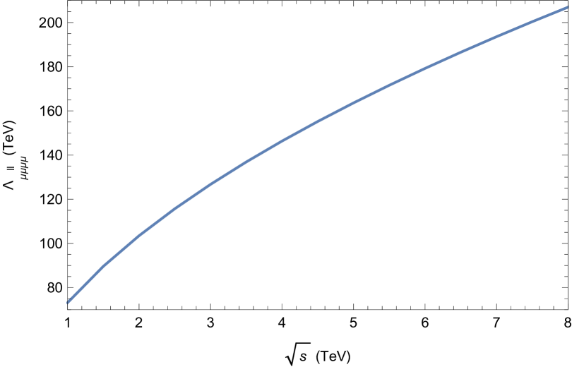
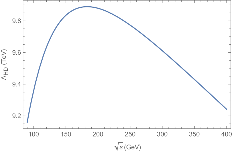
Figure 1: The $\sqrt{s}$ dependence of the bounds on $\Lambda_{\ell\ell,\mu\mu\mu\mu}$ (left) and $\Lambda_{HD}$ (right) at the $\mu^{+}\mu^{+}$ collider. The initial helicity is set to be $s_{1}=s_{2}=1$.

We need to check whether the $\theta$ dependence of the new physics contribution is different from the SM contribution, because the luminosity would be measured by using the same scattering process. We checked that the ratio of the new physics contribution to the SM one has nontrivial dependence on $\theta$. See fig. 2.

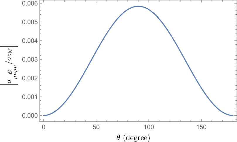
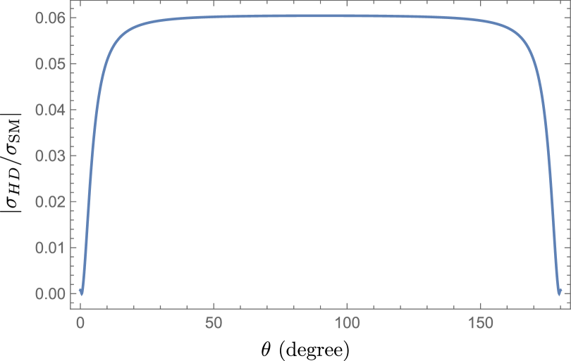
Figure 2: The $\theta$ dependence of the ratio of the new physics contribution to the SM one for $C_{\ell\ell,\mu\mu\mu\mu}=1/(100\,\text{TeV})^{2}$ (left) and $C_{HD}=1/(\text{TeV}^{2})$ (right) at the $\mu^{+}\mu^{+}$ collider of $\sqrt{s}=2\,\text{TeV}$. The initial helicity is set to be $s_{1}=s_{2}=1$.

4 Precision measurements at an $e^{-}\mu^{+}$ collider

Now we consider the scattering $e^{-}\mu^{+}\to e^{-}\mu^{+}$. The SM cross section is given through

$$\sum_{s_{3},s_{4}}|\mathcal{M}_{s_{1}s_{2}}^{\rm SM}|^{2}$$

$$=\sum_{i,j}g^{i}_{s_{1}}g^{j}_{s_{1}}g^{i}_{-s_{2}}g^{j}_{-s_{2}}8[(1+s_{1}s_{2})(p_{1}\cdot p_{2})(p_{3}\cdot p_{4})+(1-s_{1}s_{2})(p_{1}\cdot p_{4})(p_{2}\cdot p_{3})]$$

$$\quad\times\frac{1}{(p_{1}-p_{3})^{2}-M_{i}^{2}}\frac{1}{(p_{1}-p_{3})^{2}-M_{j}^{2}}.$$ (52)

We label the initial state $e^{-}$ by $(p_{1},s_{1})$, the initial state $\mu^{+}$ by $(p_{2},s_{2})$, the final state $e^{-}$ by $(p_{3},s_{3})$ and the final state $\mu^{+}$ by $(p_{4},s_{4})$.

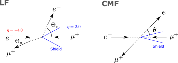
Figure 3: The angular range in which the electron and the muon go in the events we used. The left (right) figure represents the laboratory (center-of-mass) frame.

In this analysis, we use the events where both an electron and a muon are observed in a certain range of angles. We require both electron and muon go into the range of about $15.4^{\circ}$ – $178^{\circ}$ in the laboratory frame. This requirement corresponds to setting the range of pseudo rapidity to be $-4<\eta<2$. (See fig. 3.) The asymmetric angular region is motivated by the fact that we need to place a shield to protect the detector from decay products of the beam muons [23]. Although the detectability of the muons flying in the direction of the shield depends on the design of the detector, we take a conservative assumption that the particles flying into that angular region are not detected. However, since the produced particles tend to go in a direction of the electron beam side due to the beam energies, this shield does not hinder us from catching events very much. The practically important factor is how widely we can catch events on the electron beam side. See fig. 4 for the $\eta_{max}$ dependence of the bounds on $\Lambda_{HD}$.

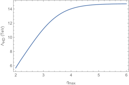
Figure 4: The $\eta$ cut (electron beam side) dependence of the bounds on $\Lambda_{HD}$ for the $e^{-}\mu^{+}$ collider of the initial energy $E_{e}=30\,\text{GeV}$ and $E_{\mu}=1\,\text{TeV}$.

In this analysis, we could obtain both the histograms concerning electrons and muons. However, since we expect better angular resolution for electrons, we only use the electron histogram. As a result of the requirement mentioned above, the angular range is determined as $62.8^{\circ}\lesssim\Theta_{e}\lesssim 178^{\circ}$. We summarize kinematic formulas in App. A.

The constraints we can obtain are summarized in tab. 2. We assume the integrated luminosity $\int\mathcal{L}dt=1~{}{\rm ab}^{-1}$.

	RR	RL	LR	LL
$C_{HWB}$	6.9 TeV	24 TeV	26 TeV	6.9 TeV
$C_{HD}$	6.8 TeV	9.0 TeV	14 TeV	6.8 TeV
$C_{H\ell}^{(1)}$	15 TeV	0	20 TeV	15 TeV
$C_{H\ell}^{(3)}$	20 TeV	18 TeV	35 TeV	20 TeV
$C_{He}$	16 TeV	19 TeV	0	16 TeV
$C_{\ell\ell}$	9.6 TeV	13 TeV	43 TeV	9.6 TeV
$C^{\prime\prime}_{\ell\ell}$	0	0	47 TeV	0
$C_{e\mu}$	0	66 TeV	0	0
$C_{\begin{subarray}{c}\ell e\\ ee\mu\mu\end{subarray}}$	0	0	0	44 TeV
$C_{\begin{subarray}{c}\ell e\\ \mu\mu ee\end{subarray}}$	44 TeV	0	0	0

Table 2: Constraints on SMEFT operators at two-sigma level. $E_{e}=30$ GeV and $E_{\mu}=1$ TeV, which amounts to $\sqrt{s}=346$ GeV. The bin size for $\Theta_{e}$ is taken as $1^{\circ}$. We require both muon and electron to go into the range of $15.4^{\circ}\lesssim\Theta\lesssim 178^{\circ}$, corresponding to $\eta_{max}=2$ for the muon beam side and $\eta_{max}=4$ for the electron beam side. As a result, the angle range of the electron is $62.8^{\circ}\lesssim\Theta_{e}\lesssim 178^{\circ}$.

It is worth noting that the constraints except for on four-fermion operators are stronger than at the $\mu^{+}\mu^{+}$ collider. The $\sqrt{s}$ dependence of the bounds and the $\theta$ dependence of the ratio of the new physics contribution to the SM, respectively, are given in figs. 5 and 6 for $C_{HD}$.

Figure 5: The $\sqrt{s}$ dependence of the bounds on $\Lambda_{HD}$ for the $e^{-}\mu^{+}$ collider. The initial helicity is given as $s_{1}=-1,s_{2}=1$. We assume the constant ratio $E_{\mu}/E_{e}=1000/30$ in drawing the figure.

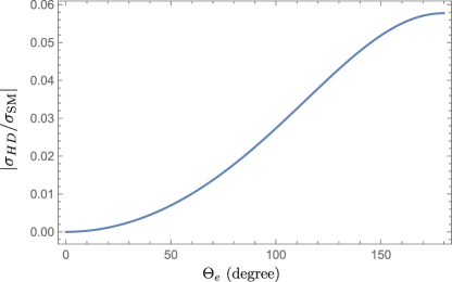
Figure 6: The $\Theta_{e}$ dependence of the ratio of the new physics contribution to the SM one for $C_{HD}=1/(\text{TeV}^{2})$ for the $e^{-}\mu^{+}$ collider. The initial helicity is given as $s_{1}=-1,s_{2}=1$.

5 Comparison to the current limits

We compare the above expected constraints with the current constraints. In Figs. 7 and 8, our results are compared with the current bounds given by Table 1 of ref. [24]. Here their “Individual” result is referred. Constraints on all the operators relevant to this study are expected to be improved. In particular, constraints on four-fermion interactions can be drastically improved.

Our study is relevant to studies which explain the recent $W$ boson mass anomaly [25] using SMEFT. Our study shows that the coefficients relevant to the $W$ boson mass formula eq. (40) can be studied in the scattering processes. In ref. [24], it is shown that non-zero $C_{HD}$ (with the other coefficients set to zero) may explain the anomaly. In this scenario, $C_{HD}$ was determined as $C_{HD}=-[0.035,0.019]/({\rm TeV}^{2})$ with the error $\delta C_{HD}=0.012/({\rm TeV}^{2})$ at the two-sigma level. Our study shows that the error of $C_{HD}$ can be reduced to $\delta C_{HD}\simeq 0.005/({\rm TeV}^{2})$. Therefore, this improvement can show more clearly whether $C_{HD}$ deviates from zero or not. (In addition, we may be able to measure $M_{W}$ directly at these new collider experiments.)

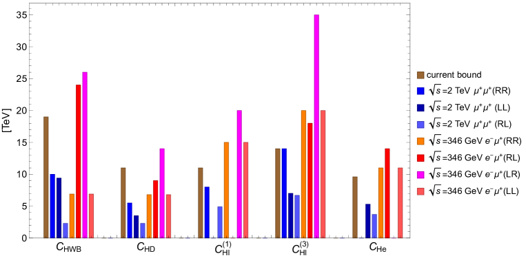
Figure 7: The current constraint and expected constraints from various scattering processes at $\mu$TRISTAN.

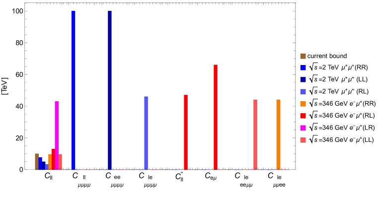
Figure 8: The current constraint and expected constraints from various scattering processes at $\mu$TRISTAN.

6 Summary

Lepton colliders are known to be quite powerful for precision measurements. There have been extensive discussions of $e^{+}e^{-}$, $\mu^{+}\mu^{-}$, and $e^{-}e^{-}$ colliders as next generation colliders. In this paper, we studied the $\mu^{+}$ based colliders as realistic muon beams can possibly be achieved much earlier than $\mu^{-}$ by using the technology of the ultra-cold muons.

We assumed that the energy of the $\mu^{+}$ beam to be 1 TeV which is discussed as the design parameter of $\mu$TRISTAN [17] with the main ring of circumference of 3 km. In the $\mu^{+}\mu^{+}$ collider option, we find that one can probe the new physics interactions up to 100 TeV. This means that, for example, effects of new gauge interactions of the muon can be seen up to the symmetry breaking scale of $O(100)$ TeV.

We also studied the reach of the $\mu^{+}e^{-}$ collider with the energy of the electron to be 30 GeV. This option is motivated by the measurements of the coupling of the Higgs boson, which is copiously produced through the $W$ boson fusion process. We find that the running with such an energy is also optimized for the electroweak precision measurements, and one can improve the constraints for $C_{HWB}$, $C_{HD}$, $C_{Hl}$ and $C_{He}$.

We worked at tree level for the calculation of the SM processes. This is sufficient to approximately understand the potential (best) reach of new physics scale. However, it would be necessary to sufficiently suppress systematic uncertainties of SM predictions by performing loop-level calculations for actual analyses and for more precise estimate of the reach. See e.g. ref. [26] for recent development in the SM calculation.

The energy of the muon beam can be much higher for a larger ring. In that case, the sensitivity to four-lepton operators gets much better. For other operators involving the Higgs fields, the modification of the Higgs coupling would be more important at high energy. In addition, one can also hope to find new particles directly. Clearly, the development of the muon acceleration technology will be a quite important key for future particle physics.

Appendix A The laboratory frame coordinates for the $\mu^{+}e^{-}$ collider

In the $\mu^{+}e^{-}$ collider, we have to note that beam energies are asymmetric. We give some formulae concerning kinematics. In the center-of-mass frame, the momenta are given by

$$p_{1}=\frac{\sqrt{s}}{2}\begin{pmatrix}1\\ 0\\ 0\\ 1\end{pmatrix},\quad{}p_{2}=\frac{\sqrt{s}}{2}\begin{pmatrix}1\\ 0\\ 0\\ -1\end{pmatrix},\quad{}p_{3}=\frac{\sqrt{s}}{2}\begin{pmatrix}1\\ 0\\ \sin{\theta}\\ \cos{\theta}\end{pmatrix},\quad{}p_{4}=\frac{\sqrt{s}}{2}\begin{pmatrix}1\\ 0\\ -\sin{\theta}\\ -\cos{\theta}\end{pmatrix}.$$ (A.1)

The matrix for transforming to the laboratory frame is given by

$$M=\begin{pmatrix}\gamma&0&0&\beta\gamma\\ 0&1&0&0\\ 0&0&1&0\\ \beta\gamma&0&0&\gamma\end{pmatrix}.$$ (A.2)

That is, the momenta in the laboratory frame is given by $p^{\prime}_{1}=Mp_{1}$ and so on. The boost factor is obtained from

$$E_{e}=\frac{\sqrt{s}}{2}\gamma(1+\beta),\quad{}E_{\mu}=\frac{\sqrt{s}}{2}\gamma(1-\beta),$$ (A.3)

where $\beta$ is explicitly given by

$$\beta=\frac{1-\frac{4E_{\mu}^{2}}{s}}{1+\frac{4E_{\mu}^{2}}{s}}=\frac{E_{e}-E_{\mu}}{E_{e}+E_{\mu}}.$$ (A.4)

The angle $\Theta_{\mu}$, in which the final muon goes in the laboratory frame, is given by

$$-\cos{\Theta}_{\mu}=\frac{p_{4,z}^{\prime}}{|\vec{p}^{\prime}_{4}|}=\frac{\gamma(\beta-\cos{\theta})}{\sqrt{\sin^{2}{\theta}+\gamma^{2}(\beta-\cos{\theta})^{2}}},$$ (A.5)

which reads

$$\cos{\theta}=\frac{-\beta\gamma^{2}\sin^{2}{\Theta_{\mu}}-\cos{\Theta_{\mu}}}{-\gamma^{2}+\cos{\Theta_{\mu}}^{2}(-1+\gamma^{2})}.$$ (A.6)

Then we have

$$dy=d(\frac{1-\cos{\theta}}{2})=-\frac{d(\cos{\theta})}{2}=-\frac{1}{2}\frac{\gamma^{2}-2\beta\gamma^{2}\cos{\Theta_{\mu}}+(\gamma^{2}-1)\cos{\Theta_{\mu}}^{2}}{(\gamma^{2}-(\gamma^{2}-1)\cos{\Theta_{\mu}}^{2})^{2}}d(\cos{\Theta_{\mu}}).$$ (A.7)

The angle of the final electron in the laboratory frame, $\Theta_{e}$, is given similarly as

$$\cos{\Theta_{e}}=\frac{p_{3,z}^{\prime}}{|\vec{p}^{\prime}_{3}|}=\frac{\gamma(\beta+\cos{\theta})}{\sqrt{\sin^{2}{\theta}+\gamma^{2}(\beta+\cos{\theta})^{2}}},$$ (A.8)

from which the following relations can be obtained:

$$\cos{\theta}=\frac{\beta\gamma^{2}\sin^{2}{\Theta_{e}}-\cos{\Theta_{e}}}{-\gamma^{2}+\cos{\Theta_{e}}^{2}(-1+\gamma^{2})},$$ (A.9)

$$dy=-\frac{1}{2}\frac{\gamma^{2}+2\beta\gamma^{2}\cos{\Theta_{e}}+(\gamma^{2}-1)\cos{\Theta_{e}}^{2}}{(\gamma^{2}-(\gamma^{2}-1)\cos{\Theta_{e}}^{2})^{2}}d(\cos{\Theta_{e}}).$$ (A.10)

References

- [1] S. Schael et al., Precision electroweak measurements on the resonance, Phys. Rept., vol. 427, pp. 257–454, 2006, doi:10.1016/j.physrep.2005.12.006, arXiv:hep-ex/0509008.
- [2] Precision Electroweak Measurements and Constraints on the Standard Model, 12 2010, arXiv:1012.2367 [hep-ex].
- [3] S. Schael et al., Electroweak Measurements in Electron-Positron Collisions at W-Boson-Pair Energies at LEP, Phys. Rept., vol. 532, pp. 119–244, 2013, doi:10.1016/j.physrep.2013.07.004, arXiv:1302.3415 [hep-ex].
- [4] E. Derman and W. J. Marciano, Parity Violating Asymmetries in Polarized Electron Scattering, Annals Phys., vol. 121, p. 147, 1979, doi:10.1016/0003-4916(79)90095-2.
- [5] A. Czarnecki and W. J. Marciano, Electroweak radiative corrections to polarized Moller scattering asymmetries, Phys. Rev. D, vol. 53, pp. 1066–1072, 1996, doi:10.1103/PhysRevD.53.1066, arXiv:hep-ph/9507420.
- [6] M. J. Ramsey-Musolf, Low-energy parity violation and new physics, Phys. Rev. C, vol. 60, p. 015501, 1999, doi:10.1103/PhysRevC.60.015501, arXiv:hep-ph/9903264.
- [7] A. Czarnecki and W. J. Marciano, Polarized Moller scattering asymmetries, Int. J. Mod. Phys. A, vol. 15, pp. 2365–2376, 2000, doi:10.1016/S0217-751X(00)00243-0, arXiv:hep-ph/0003049.
- [8] P. L. Anthony et al., Precision measurement of the weak mixing angle in Moller scattering, Phys. Rev. Lett., vol. 95, p. 081601, 2005, doi:10.1103/PhysRevLett.95.081601, arXiv:hep-ex/0504049.
- [9] K. S. Kumar, S. Mantry, W. J. Marciano, and P. A. Souder, Low Energy Measurements of the Weak Mixing Angle, Ann. Rev. Nucl. Part. Sci., vol. 63, pp. 237–267, 2013, doi:10.1146/annurev-nucl-102212-170556, arXiv:1302.6263 [hep-ex].
- [10] J. Benesch et al., The MOLLER Experiment: An Ultra-Precise Measurement of the Weak Mixing Angle Using M\oller Scattering, 11 2014, arXiv:1411.4088 [nucl-ex].
- [11] W. Buchmuller and D. Wyler, Effective Lagrangian Analysis of New Interactions and Flavor Conservation, Nucl. Phys. B, vol. 268, pp. 621–653, 1986, doi:10.1016/0550-3213(86)90262-2.
- [12] B. Grzadkowski, M. Iskrzynski, M. Misiak, and J. Rosiek, Dimension-Six Terms in the Standard Model Lagrangian, JHEP, vol. 10, p. 085, 2010, doi:10.1007/JHEP10(2010)085, arXiv:1008.4884 [hep-ph].
- [13] I. Brivio and M. Trott, The Standard Model as an Effective Field Theory, Phys. Rept., vol. 793, pp. 1–98, 2019, doi:10.1016/j.physrep.2018.11.002, arXiv:1706.08945 [hep-ph].
- [14] J. Ellis, M. Madigan, K. Mimasu, V. Sanz, and T. You, Top, Higgs, Diboson and Electroweak Fit to the Standard Model Effective Field Theory, JHEP, vol. 04, p. 279, 2021, doi:10.1007/JHEP04(2021)279, arXiv:2012.02779 [hep-ph].
- [15] The International Linear Collider Technical Design Report - Volume 1: Executive Summary, 6 2013, arXiv:1306.6327 [physics.acc-ph].
- [16] J. Ellis and T. You, Sensitivities of Prospective Future e+e- Colliders to Decoupled New Physics, JHEP, vol. 03, p. 089, 2016, doi:10.1007/JHEP03(2016)089, arXiv:1510.04561 [hep-ph].
- [17] Y. Hamada, R. Kitano, R. Matsudo, H. Takaura, and M. Yoshida, TRISTAN, PTEP, vol. 2022, no. 5, p. 053B02, 2022, doi:10.1093/ptep/ptac059, arXiv:2201.06664 [hep-ph].
- [18] Y. Kondo et al., Re-Acceleration of Ultra Cold Muon in J-PARC Muon Facility, in 9th International Particle Accelerator Conference, 6 2018.
- [19] M. Abe et al., A New Approach for Measuring the Muon Anomalous Magnetic Moment and Electric Dipole Moment, PTEP, vol. 2019, no. 5, p. 053C02, 2019, doi:10.1093/ptep/ptz030, arXiv:1901.03047 [physics.ins-det].
- [20] M. E. Peskin and T. Takeuchi, A New constraint on a strongly interacting Higgs sector, Phys. Rev. Lett., vol. 65, pp. 964–967, 1990, doi:10.1103/PhysRevLett.65.964.
- [21] G. Altarelli and R. Barbieri, Vacuum polarization effects of new physics on electroweak processes, Phys. Lett. B, vol. 253, pp. 161–167, 1991, doi:10.1016/0370-2693(91)91378-9.
- [22] R. Alonso, E. E. Jenkins, A. V. Manohar, and M. Trott, Renormalization Group Evolution of the Standard Model Dimension Six Operators III: Gauge Coupling Dependence and Phenomenology, JHEP, vol. 04, p. 159, 2014, doi:10.1007/JHEP04(2014)159, arXiv:1312.2014 [hep-ph].
- [23] N. Bartosik et al., Detector and Physics Performance at a Muon Collider, JINST, vol. 15, no. 05, p. P05001, 2020, doi:10.1088/1748-0221/15/05/P05001, arXiv:2001.04431 [hep-ex].
- [24] E. Bagnaschi, J. Ellis, M. Madigan, K. Mimasu, V. Sanz, and T. You, SMEFT Analysis of , 4 2022, arXiv:2204.05260 [hep-ph].
- [25] T. Aaltonen et al., High-precision measurement of the W boson mass with the CDF II detector, Science, vol. 376, no. 6589, pp. 170–176, 2022, doi:10.1126/science.abk1781.
- [26] S. G. Bondarenko, L. V. Kalinovskaya, L. A. Rumyantsev, and V. L. Yermolchyk, One-loop electroweak radiative corrections to polarized Møller scattering, 3 2022, arXiv:2203.10538 [hep-ph].