A curious identity in connection with saddle-point method and Stirling’s formula

Abstract.

We prove the curious identity in the sense of formal power series:

$$\int_{-\infty}^{\infty}[y^{m}]\exp\left(-\frac{t^{2}}{2}+\sum_{j\geqslant 3}\frac{(it)^{j}}{j!}\,y^{j-2}\right)\mathrm{d}t=\int_{-\infty}^{\infty}[y^{m}]\exp\left(-\frac{t^{2}}{2}+\sum_{j\geqslant 3}\frac{(it)^{j}}{j}\,y^{j-2}\right)\mathrm{d}t,$$

for $m=0,1,\dots$, where $[y^{m}]f(y)$ denotes the coefficient of $y^{m}$ in the Taylor expansion of $f$. The generality of this identity from the perspective of saddle-point method is also examined.

1. Introduction

The following unusual identity was discovered through different manipulations of the saddle-point method in order to derive Stirling’s formula, which has a huge literature since de Moivre’s and Stirling’s pioneering analysis in the early eighteenth century; see for example the survey [1] (and the references therein) and the book [9] for five different analytic proofs. While the identity can be deduced from known expansions for $n!$ (e.g., [3, 23]), the formulation, as well as the proof given here, is of independent interest per se. Denote by $[y^{m}]f(y)$ the coefficient of $y^{m}$ in the Taylor expansion of $f$.

Theorem 1.1.

Let

$$c_{m}:=\frac{1}{\sqrt{2\pi}}\int_{-\infty}^{\infty}[y^{m}]\exp\biggl{(}{-\frac{t^{2}}{2}+\sum_{j\geqslant 3}\frac{(it)^{j}}{\hbox{\pagecolor{hili}$j!$}}\,y^{j-2}}\biggr{)}{\,\rm d}t,$$ (1)

and

$$d_{m}:=\frac{1}{\sqrt{2\pi}}\int_{-\infty}^{\infty}[y^{m}]\exp\biggl{(}{-\frac{t^{2}}{2}+\sum_{j\geqslant 3}\frac{(it)^{j}}{\hbox{\pagecolor{hili}$j$}}\,y^{j-2}}\biggr{)}{\,\rm d}t.$$ (2)

Then

$$c_{m}=d_{m}\qquad(m=0,1,\dots).$$ (3)

When $m$ is odd, $c_{m}=d_{m}=0$ because the coefficient of $y^{m}$ contains only odd powers of $t$. When $m=2l$ is even, the identity (3) can be written explicitly as follows:

$$c_{2l} =\sum_{1\leqslant h\leqslant 2l}\frac{(-1)^{l+h}(2l+2h)!}{(l+h)!2^{l+h}}\sum_{\begin{subarray}{c}j_{1}+2j_{2}+\cdots+2lj_{2l}=2l\\ j_{1}+\cdots+j_{2l}=h\end{subarray}}\frac{1}{j_{1}!\cdots j_{2l}!\cdot\hbox{\pagecolor{hili}$3!^{j_{1}}4!^{j_{2}}\cdots(2l+2)!^{j_{2l}}$}}$$

$$=\sum_{1\leqslant h\leqslant 2l}\frac{(-1)^{l+h}(2l+2h)!}{(l+h)!2^{l+h}}\sum_{\begin{subarray}{c}j_{1}+2j_{2}+\cdots+2lj_{2l}=2l\\ j_{1}+\cdots+j_{2l}=h\end{subarray}}\frac{1}{j_{1}!\cdots j_{2l}!\cdot\hbox{\pagecolor{hili}$3^{j_{1}}4^{j_{2}}\cdots(2l+2)^{j_{2l}}$}}$$

$$=d_{2l}.$$

In particular,

$$\{c_{2l}\}_{l\geqslant 0}=\left\{1,-\frac{1}{12},\frac{1}{288},\frac{139}{51840},-\frac{571}{2488320},-\frac{163879}{209018880},\cdots\right\},$$

which are modulo sign the coefficients appearing in the asymptotic expansion of Stirling’s formula; see [8, §1.18] or [22, A001163, A001164]:

$$\frac{1}{n!}\sim\frac{e^{n}n^{-n-\frac{1}{2}}}{\sqrt{2\pi}}\sum_{m\geqslant 0}c_{2m}n^{-m},\quad\text{or}\quad n!\sim\sqrt{2\pi}e^{-n}n^{n+\frac{1}{2}}\sum_{m\geqslant 0}(-1)^{m}c_{2m}n^{-m}.$$ (4)

These Stirling coefficients have been extensively studied in the literature; see, e.g., [6, §8.2], and [2, 15, 23, 18], and the references cited there.

On the other hand, the integral in (1) without the coefficient-extraction operator $[y^{m}]$ is divergent for $y\in\mathbb{R}$ due to periodicity:

$$\int_{-\infty}^{\infty}\exp\biggl{(}{-\frac{t^{2}}{2}+\sum_{j\geqslant 3}\frac{(it)^{j}}{j!}\,y^{j-2}}\biggr{)}{\,\rm d}t=\int_{-\infty}^{\infty}\exp\biggl{(}{\frac{e^{ity}-1-ity}{y^{2}}}\biggr{)}{\,\rm d}t,$$

while that in (2) is absolutely convergent for real $|y|<1$:

$$\int_{-\infty}^{\infty}\exp\biggl{(}{-\frac{t^{2}}{2}+\sum_{j\geqslant 3}\frac{(it)^{j}}{j}\,y^{j-2}}\biggr{)}{\,\rm d}t=\int_{-\infty}^{\infty}\bigl{(}{1-ity}\bigr{)}^{-y^{-2}}e^{-it/y}{\,\rm d}t.$$

Proof of Theorem 1.1.

For convenience, we write

$$f_{n}\thickapprox g_{n}\quad\text{when}\quad f_{n}=g_{n}+O\bigl{(}{e^{-\varepsilon n}}\bigr{)},$$

for some generic $\varepsilon>0$ whose value is immaterial.

The standard asymptotic expansion

We begin with the Cauchy integral representation for $n!^{-1}$:

$$\frac{1}{n!}=\frac{1}{2\pi i}\oint_{|z|=n}z^{-n-1}e^{z}{\,\rm d}z,$$

where the integration contour is the circle with radius $|z|=n$. The standard application of the saddle-point method (see [9, p. 555]) proceeds by first making the change of variables $z\mapsto ne^{u}$, giving

$$\frac{e^{-n}n^{n}}{n!} =\frac{1}{2\pi i}\int_{-\pi i}^{\pi i}e^{n(e^{u}-1-u)}{\,\rm d}u\thickapprox\frac{1}{2\pi i}\int_{-\varepsilon i}^{\varepsilon i}e^{n(e^{u}-1-u)}{\,\rm d}u.$$ (5)

Now by the change of variables $u=\frac{it}{\sqrt{n}}$, we have

$$\frac{1}{2\pi i}\int_{-\varepsilon i}^{\varepsilon i}e^{n(e^{u}-1-u)}{\,\rm d}u =\frac{1}{2\pi\sqrt{n}}\int_{-\varepsilon\sqrt{n}}^{\varepsilon\sqrt{n}}\exp\biggl{(}{-\frac{t^{2}}{2}+\sum_{j\geqslant 3}\frac{(it)^{j}}{j!}\,n^{-\frac{1}{2}j+1}}\biggr{)}{\,\rm d}t.$$

If we choose $\varepsilon=\varepsilon_{n}=n^{-\frac{2}{5}}$, say, then $n\varepsilon_{n}^{2}\to\infty$ and $n\varepsilon_{n}^{j}\to 0$ for $j\geqslant 3$, so that the series on the right-hand side is small on the integration path; we can then expand the exponential of this series in decreasing powers of $n$, and then extending the integration limits to infinity, yielding the expansion (4) with $c_{2m}$ expressed in the formal power series form (1). See [9, Ex. VIII.3; p. 555 et seq.] for technical details.

On the other hand, a more effective means of computing $c_{2m}$ is to make first the change of variables $e^{u}-1-u=\frac{1}{2}v^{2}$ in the rightmost integral in (5), where $u=u(v)$ is positive when $v$ is and is analytic in $|v|\leqslant\varepsilon$; see [26, § 3.6.3]. Then

$$\frac{e^{-n}n^{n}}{n!}\thickapprox\frac{1}{2\pi i}\int_{-\varepsilon i}^{\varepsilon i}e^{\frac{1}{2}nv^{2}}g(v){\,\rm d}v=\frac{1}{2\pi}\int_{-\varepsilon}^{\varepsilon}e^{-\frac{1}{2}nt^{2}}g(it){\,\rm d}t,$$

where $g(v):=\frac{{\,\rm d}u}{{\,\rm d}v}$ is analytic in $|v|\leqslant\varepsilon$. By Lagrange inversion formula (see [9, p. 732]),

$$g_{m}:=[v^{m}]g(v)=[t^{m}]\biggl{(}{\frac{\frac{1}{2}t^{2}}{e^{t}-1-t}}\biggr{)}^{\frac{1}{2}(m+1)}\qquad(m=0,1,\dots).$$ (6)

Then a direct application of Watson’s Lemma (see [28, §1.5]) gives the asymptotic expansion

$$\frac{1}{n!}\thickapprox\frac{e^{n}n^{-n}}{2\pi}\sum_{m\geqslant 0}g_{2m}\int_{-\infty}^{\infty}e^{-\frac{1}{2}nt^{2}}(it)^{2m}{\,\rm d}t\thickapprox\frac{e^{n}n^{-n}}{\sqrt{2\pi n}}\sum_{m\geqslant 0}\bar{g}_{2m}n^{-m},$$ (7)

where

$$\{\bar{g}_{2m}\}_{m\geqslant 0}:=\Bigl{\{}g_{2m}\frac{(-1)^{m}(2m)!}{m!2^{m}}\Bigr{\}}_{m\geqslant 0}=\Bigl{\{}1,-\frac{1}{12},\frac{1}{288},\frac{139}{51840},-\frac{571}{2488320},\cdots\Bigr{\}}.$$

We then obtain the relation

$$c_{2m}=\bar{g}_{2m}=g_{2m}\frac{(-1)^{m}(2m)!}{m!2^{m}}.$$ (8)

Second asymptotic expansion

It is well known that $n!^{-1}$ has the alternative Laplace integral representation (see [27, p. 246]):

$$\frac{1}{n!}=\frac{1}{2\pi i}\int_{R-i\infty}^{R+i\infty}z^{-n-1}e^{z}{\,\rm d}z\qquad(R>0),$$

so that, by the change of variables $z=R(1+x)$, where $R=n+1$,

$$\frac{e^{-n-1}(n+1)^{n}}{n!} =\frac{1}{2\pi i}\int_{-i\infty}^{i\infty}e^{-(n+1)(\log(1+x)-x)}{\,\rm d}x$$

$$\thickapprox\frac{1}{2\pi i}\int_{-\varepsilon i}^{\varepsilon i}e^{-(n+1)(\log(1+x)-x)}{\,\rm d}x.$$

Now by the change of variables $x=\frac{it}{\sqrt{n+1}}$, we have

$$\frac{1}{2\pi i}\int_{-\varepsilon i}^{\varepsilon i}e^{-(n+1)(\log(1+x)-x)}{\,\rm d}x$$

$$\qquad=\frac{1}{2\pi\sqrt{n+1}}\int_{-\varepsilon\sqrt{n+1}}^{\varepsilon\sqrt{n+1}}\exp\biggl{(}{-\frac{t^{2}}{2}+\sum_{j\geqslant 3}\frac{(it)^{j}}{j}\,(n+1)^{-\frac{1}{2}j+1}}\biggr{)}{\,\rm d}t.$$

By a similar procedure described above, we then deduce the asymptotic expansion

$$\frac{1}{n!}\sim\frac{e^{n+1}(n+1)^{-n-\frac{1}{2}}}{\sqrt{2\pi}}\sum_{m\geqslant 0}d_{2m}(n+1)^{-m},$$ (9)

where $d_{m}$ is given in (2); compare (7).

On the other hand, by the change of variables $\log(1+x)-x=-\frac{1}{2}y^{2}$ ($y>0$ when $x>0$), we have

$$\frac{e^{-n-1}(n+1)^{n}}{n!} \thickapprox\frac{1}{2\pi i}\int_{-\varepsilon i}^{\varepsilon i}e^{\frac{1}{2}(n+1)y^{2}}h(y){\,\rm d}y=\frac{1}{2\pi}\int_{-\varepsilon}^{\varepsilon}e^{-\frac{1}{2}(n+1)t^{2}}h(it){\,\rm d}t,$$

where $h(y)=\frac{{\,\rm d}x}{{\,\rm d}y}$ is analytic in $|y|\leqslant\varepsilon$. Again, by Lagrange inversion formula,

$$h_{m}:=[y^{m}]h(y)=[y^{m}]\biggl{(}{\frac{\frac{1}{2}y^{2}}{y-\log(1+y)}}\biggr{)}^{\frac{1}{2}(m+1)}\qquad(m=0,1,\dots).$$ (10)

Although the definition of $h_{m}$ looks very different from that of $g_{m}$ (see (6)), their numerical values coincide except for $m=1$:

$m$	$0$	$1$	$2$	$3$	$4$	$5$	$6$	$7$	$8$	$9$
$g_{m}$	$1$	$-\frac{1}{3}$	$\frac{1}{12}$	$-\frac{2}{135}$	$\frac{1}{864}$	$\frac{1}{2835}$	$-\frac{139}{777600}$	$\frac{1}{25515}$	$-\frac{571}{261273600}$	$-\frac{281}{151559100}$
$h_{m}$		$\frac{2}{3}$

We thus deduce the relation

$$d_{2m}:=h_{2m}\frac{(-1)^{m}(2m)!}{m!2^{m}},$$

which is easily computable by (10).

Equality of the two expansions

We next prove that

$$g_{m}=h_{m}\qquad(m\geqslant 0;m\neq 1),$$ (11)

where $g_{m}$ and $h_{m}$ are defined in (6) and (10), respectively. Note that for $m\geqslant 0$

$$g_{m}=[s^{m}]\frac{\varphi(s)^{m+1}}{1+s},\quad\text{with}\quad\varphi(s):=\biggl{(}{\frac{s^{2}}{2(s-\log(1+s))}}\biggr{)}^{\frac{1}{2}},$$ (12)

by a direct change of variables $s=e^{t}-1$. Thus we show that

$$[s^{m}]\frac{\varphi(s)^{m+1}}{1+s}=[s^{m}]\varphi(s)^{m+1}$$

for $m\neq 1$, or, equivalently,

$$[s^{m-1}]\frac{\varphi(s)^{m+1}}{1+s}=0\qquad(m\geqslant 0,m\neq 1).$$ (13)

Since $m=0,1$ are easily checked, we assume $m\geqslant 2$. By the relation

$$\frac{s\varphi^{\prime}(s)}{\varphi(s)}=1-\frac{\varphi(s)^{2}}{1+s},$$

we have

$$[s^{m-1}]\frac{\varphi(s)^{m+1}}{1+s} =[s^{m-1}]\bigl{(}{\varphi(s)^{m-1}-s\varphi(s)^{m-2}\varphi^{\prime}(s)}\bigr{)}$$

$$=h_{m-1}-[s^{m-2}]\varphi(s)^{m-2}\varphi^{\prime}(s).$$

Now

$$[s^{m-2}]\varphi(s)^{m-2}\varphi^{\prime}(s) =[s^{m-2}]\frac{{\,\rm d}}{{\,\rm d}s}\frac{\varphi(s)^{m-1}}{m-1}=[s^{m-1}]\varphi(s)^{m-1}=h_{m-1},$$

which proves (13), and in turn (11). Consequently, $c_{m}=d_{m}$ for $m\geqslant 0$, implying (3). ∎

It is known that (see [6, §8.2] and [2])

$$g_{2m}\sim(-1)^{l+1}\sqrt{2\pi}(4\pi)^{-2l}\times\begin{cases}\frac{1}{24}l^{-\frac{3}{2}},&\text{if }m=2l;\\ 2l^{-\frac{1}{2}},&\text{if }m=2l-1.\end{cases}$$

This type of asymptotic behaviors is unusual for functions of Lagrangean type; see [13] or § 3.

2. Asymptotic expansions by saddle-point method

Quoted from [9, p. 551]

Saddle-point method $$= +$$ Choice of contour Laplace’s method.

Similar to its real-variable counterpart, the saddle-point method is a general strategy rather than a completely deterministic algorithm, since many choices are left open in the implementation of the method concerning details of the contour and choices of its splitting into pieces.

2.1. $z=re^{i\theta}$ or $z=R(1+it)$?

The two uses above (with $z=re^{i\theta}$ or $z=R(1+it)$) of the saddle-point method for coefficient integrals of the form

$$a_{n}:=\frac{1}{2\pi i}\int_{\mathscr{C}}z^{-n-1}f(z){\,\rm d}z,$$

for some contour $\mathscr{C}$ are standard in the combinatorial literature and are reminiscent of the difference between moments and factorial moments in probability; the corresponding saddle-point equations are given by

$$\frac{rf^{\prime}(r)}{f(r)}=n,\quad\text{and}\quad\frac{Rf^{\prime}(R)}{f(R)}=n+1,$$ (14)

respectively. Often the question is which one to choose and is better (numerically or in some other sense)? For example, take $f(z)=e^{e^{z}-1}$ (Bell numbers [22, A000110]); then we found both uses in the literature:

$re^{r}=n$	$Re^{R}=n+1$
[16, 25] [20, Ex. 12.2] [24, § 5.8]	[5, § 6.2] [9, pp. 560–562] [14, pp. 422–423]

In particular, Knuth [14, pp. 422–423] considers first $a_{n-1}$ and then changed $n-1$ to $n$ after deriving the corresponding asymptotic approximation.

The question of whether to use $r$ or $R$ in (14) is partly answered in [9, p. 555, footnote]: “the choice being often suggested by computational convenience.” Odlyzko in [20, p. 1184] also commented that the use of $r$ is slightly preferred because the manipulation of the other version is less elegant.

Apart from computational convenience, the numerical advantages of the expansion (9) over (7) are visible because they have the same sequence of coefficients and $(n+1)^{-m}$ is always smaller than $n^{-m}$; see also [4] for Stirling’s original expansion in decreasing powers of $n+\frac{1}{2}$. Although the numerical difference is minor for most practical uses, the same question can naturally be raised more generally for functions $f$ whose Taylor coefficients are amenable to saddle-point method (for example, exponential of Hayman admissible functions; see [21]). Indeed, such a numerical difference was already observed in the 1960s by Harris and Schoenfeld in their study of idempotent elements in symmetric semigroups [10] where $f(z)=e^{ze^{z}}$. Based on numerical calculations, they found that the saddle-point approximation

$$\frac{a_{n}}{n!} :=[z^{n}]e^{ze^{z}}$$

$$\sim\frac{R^{-n}e^{Re^{R}}}{\sqrt{2\pi Re^{R}(R^{2}+3R+1)}}\quad\text{with $R>0$ solving $R(R+1)e^{R}=n+1$,}\quad$$ (15)

is “considerably better than the approximation”

$$\frac{a_{n}}{n!}\sim\frac{r^{-n}e^{re^{r}}}{\sqrt{2\pi re^{r}(r^{2}+3r+1)}}\quad\text{with $r>0$ solving $r(r+1)e^{r}=n$.}\quad$$ (16)

Surprisingly, this is the only paper we found where such a numerical comparison between the two versions of saddle-point method was made.

In the same paper [10], Harris and Schoenfeld also argued that the reason that (15) outperforms (16) is (we change their notations to ours) “because the derivation of (15) uses a contour which passes through the saddle point of a certain integral for $a_{n}/n!$. However, Hayman’s proof of the formula yielding (16) employs a contour passing through $r=r(n)=R(n-1)$ and it therefore misses the saddle point at $R$ by $R(n)-R(n-1)\sim 1/n$.”

However, such a comparison is not quite right. In fact, the use of $r$ or $R$ in each case, after the change of variables, is optimally guided by the saddle-point principle, and thus different choices of integration contour will result in different expansions with different asymptotic scales. As we will see below in § 2.3, while the dominant term in (15) is better than that in (16) under the absolute difference measure, the use of more terms in the corresponding asymptotic expansions may change the scenario, and which expansion is numerically more precise depends on the number of terms used.

In this section, we first consider the two versions of the saddle-point method for general $f$, and then give succinct expressions for the coefficients in the corresponding asymptotic expansions. Then we discuss some examples, highlighting briefly their numerical differences.

2.2. Two asymptotic expansions by saddle-point method

Consider

$$a_{n}:=[z^{n}]e^{\phi(z)}=\frac{1}{2\pi i}\oint_{|z|=r}z^{-n-1}e^{\phi(z)}{\,\rm d}z,$$

where $\phi$ is analytic at zero. For simplicity we will simply assume that asymptotic expansions can be derived by the saddle-point method, instead of formulating general theorems for asymptotic expansions whose conditions are often very messy to the extent that in many practical cases, their justifications are not much different from working out the saddle-point method from scratch; see e.g. [11, 17, 21, 29]. In this way, we focus on the formal aspects of the coefficients and the differences between the two expansions, referring all technical details or justification to standard references such as [11, 17, 29] or [9, § VIII.5]. Then we have the following two different asymptotic expansions.

• The change of variables $z\mapsto re^{i\theta}$ (integration on a circle): let

  $$\kappa_{j}(r) :=j![s^{j}]\bigl{(}{-ns+\phi(re^{s})}\bigr{)}\qquad(j=1,2,\dots),$$

  where $\kappa_{1}(r)=0$ or $r\phi^{\prime}(r)=n$. Also $\kappa_{2}(r)=r\phi^{\prime}(r)+r^{2}\phi^{\prime\prime}(r)$. Then under proper conditions

  $$a_{n}\sim\frac{r^{-n}e^{\phi(r)}}{\sqrt{2\pi\kappa_{2}(r)}}\sum_{m\geqslant 0}c_{m}(r)\kappa_{2}(r)^{-m},$$

  where

  $$c_{m}(r):=\frac{1}{\sqrt{2\pi}}\int_{-\infty}^{\infty}e^{-\frac{1}{2}t^{2}}[y^{m}]\exp\biggl{(}{\sum_{j\geqslant 3}\frac{\kappa_{j}(r)}{j!\kappa_{2}(r)}(it)^{j}y^{\frac{1}{2}j-1}}\biggr{)}{\,\rm d}t.$$

  Alternatively, by the same analysis as above for Stirling’s formula, we also have

  $$c_{m}(r)=g_{2m}(r)\frac{(-1)^{m}(2m)!}{m!2^{m}},$$ (17)

  where

  $$g_{m}(r)=[v^{m}]\biggl{(}{\frac{\frac{1}{2}\kappa_{2}(r)v^{2}}{\phi(re^{v})-\phi(r)-r\phi^{\prime}(r)v}}\biggr{)}^{\frac{1}{2}(m+1)}.$$

  In particular (with $\kappa_{j}=\kappa_{j}(r)$),

  $$c_{1}(r) =\frac{3\kappa_{2}\kappa_{4}-5\kappa_{3}^{2}}{24\kappa_{2}^{2}},$$

  $$c_{2}(r) =-\frac{24\kappa_{2}^{3}\kappa_{6}-168\kappa_{2}^{2}\kappa_{3}\kappa_{5}-105\kappa_{2}^{2}\kappa_{4}^{2}+630\kappa_{2}\kappa_{3}^{2}\kappa_{4}-385\kappa_{3}^{4}}{1152\kappa_{2}^{4}}.$$

• The change of variables $z\mapsto R(1+it)$ (integration on a vertical line): let

  $$\lambda_{j}(R) =j![s^{j}]\bigl{(}{-(n+1)\log(1+s)+\phi(R(1+s))}\bigr{)}$$

  $$=(-1)^{j}(j-1)!R\phi^{\prime}(R)+j![s^{j}]\phi(R(1+s)),$$

  where $R\phi^{\prime}(R)=n+1$. Note that $\lambda_{2}(t)=\kappa_{2}(t)$. Then under proper conditions

  $$a_{n}\sim\frac{R^{-n}e^{\phi(R)}}{\sqrt{2\pi\lambda_{2}(R)}}\sum_{m\geqslant 0}d_{m}(R)\lambda_{2}(R)^{-m},$$

  where

  $$d_{m}(R):=\frac{1}{\sqrt{2\pi}}\int_{-\infty}^{\infty}e^{-\frac{1}{2}t^{2}}[y^{m}]\exp\biggl{(}{\sum_{j\geqslant 3}\frac{\lambda_{j}(r)}{j!\lambda_{2}(r)}(it)^{j}y^{\frac{1}{2}j-1}}\biggr{)}{\,\rm d}t.$$

  Alternatively, we also have

  $$d_{m}(R)=h_{2m}(R)\frac{(-1)^{m}(2m)!}{m!2^{m}},$$ (18)

  where

  $$h_{m}(R)=[y^{m}]\biggl{(}{\frac{\frac{1}{2}\lambda_{2}(R)y^{2}}{\phi(R(1+y))-\phi(R)-R\phi^{\prime}(R)\log(1+y)}}\biggr{)}^{\frac{1}{2}(m+1)}.$$

  In particular, (with $\lambda_{j}=\lambda_{j}(R)$)

  $$d_{1}(R) =\frac{3\lambda_{2}\lambda_{4}-5\lambda_{3}^{2}}{24\lambda_{2}^{2}},$$

  $$d_{2}(R) =-\frac{24\lambda_{2}^{3}\lambda_{6}-168\lambda_{2}^{2}\lambda_{3}\lambda_{5}-105\lambda_{2}^{2}\lambda_{4}^{2}+630\lambda_{2}\lambda_{3}^{2}\lambda_{4}-385\lambda_{3}^{4}}{1152\lambda_{2}^{4}},$$

  the expressions differing from $c_{1}(r)$ and $c_{2}(r)$ by replacing all $\kappa_{j}(r)$ by $\lambda_{j}(R)$.

2.3. Examples.

We begin with Harris and Schoenfeld’s example $\phi(z)=ze^{z}$ [10] and let $a_{n}:=n![z^{n}]e^{ze^{z}}$, the number of idempotent mappings from a set of $n$ elements into itself; see also [22, A000248]. Asymptotic expansions by saddle-point method can be justified either by checking the Harris-Schoenfeld admissibility conditions as in [10] or by showing that $ze^{z}$ is a Hayman admissible function (see [12, 21, 9]). We then compute the absolute differences between the true values and the two asymptotic expansions with varying number of terms:

$$\begin{split}\Delta_{n,M}^{(c)}&:=\frac{n^{M+1}}{(\log n)^{M+1}}\left|\frac{a_{n}}{\displaystyle\frac{r^{-n}e^{re^{r}}}{\sqrt{2\pi\kappa_{2}(r)}}}-\sum_{0\leqslant m\leqslant M}c_{m}(r)\kappa_{2}(r)^{-m}\right|,\\ \Delta_{n,M}^{(v)}&:=\frac{n^{M+1}}{(\log n)^{M+1}}\left|\frac{a_{n}}{\displaystyle\frac{R^{-n}e^{Re^{R}}}{\sqrt{2\pi\kappa_{2}(R)}}}-\sum_{0\leqslant m\leqslant M}d_{m}(R)\kappa_{2}(R)^{-m}\right|,\end{split}$$ (19)

where $r>0$ solves $r(r+1)e^{r}=n$, $R>0$ solves $R(r+1)e^{R}=n+1$, and $\kappa_{2}$ and the coefficients $c_{m}$ and $d_{m}$ can be computed by (17) and (18), respectively, with $\phi(z)=ze^{z}$. Note that $g(2m)\kappa_{2}(r)^{-m}$ grows in the order $n^{-m}(\log n)^{m}$ for $m=0,1,\dots$.

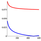
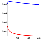
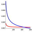
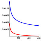
Figure 1. $\Delta_{n,M}^{(c)}$ (in red) vs $\Delta_{n,M}^{(v)}$ (in blue): $20\leqslant n\leqslant 200$ and $M=0,1,2,3,4$ (in left to right order).

From Figure 1, we see that while (15) is numerically better than its circular counterpart (16) (or $M=0$. as already observed in [10]), more terms in the asymptotic expansions show that both expansions are indeed comparable, and their numerical performance depends on the number of terms used.

We also observed a very similar pattern (as Figure 1) for Bell numbers when $\phi(z)=e^{z}-1$; see [22, A000110].

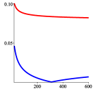
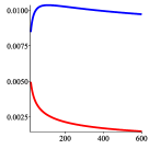
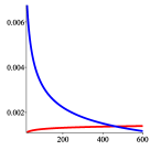
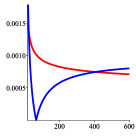
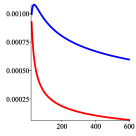
Figure 2. $\Delta_{n,M}^{(c)}$ (in red) vs $\Delta_{n,M}^{(v)}$ (in blue) in the case of Bell numbers: $15\leqslant n\leqslant 200$ and $M=0,1,2,3,4$ (in left to right order).

In the case of $\phi(z)=\frac{z}{1-z}$, $a_{n}:=n![z^{n}]e^{z/(1-z)}$ enumerates the number of partitions of $\{1,\dots,n\}$ into any number of ordered subsets; see [22, A000262]. Justification of an asymptotic expansion is straightforward and similar to integer partition problems.

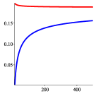
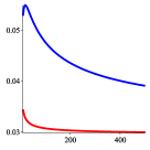
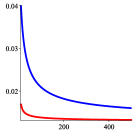
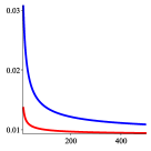
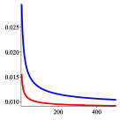
Figure 3. $\Delta_{n,M}^{(c)}$ (in red) vs $\Delta_{n,M}^{(v)}$ (in blue) in the case of $\phi(z)=\frac{z}{1-z}$: $10\leqslant n\leqslant 200$ and $M=0,1,2,3,4$ (in left to right order). Here $\Delta_{n,M}^{(\cdot)}$ is defined as in (19) but with $\frac{n^{M+1}}{(\log n)^{M+1}}$ there replaced by $n^{\frac{1}{2}(M+1)}$.

One sees that the circular version is numerically better except for $M=0$.

Finally, consider the case $\phi(z)=z+\frac{1}{2}z^{2}$, whose coefficients (times $n!$) enumerate the number of self-inverse permutations on $n$ elements; see [22, A000085]. Since all coefficients of $\phi(z)$ are positive, an asymptotic expansion by saddle-point method is possible by known results of Moser and Wyman in the 1950s [17]; see also [20]. In this case, we plot the difference $\Delta_{n,M}^{(c)}-\Delta_{n,M}^{(v)}$ because the two curves are too close to be distinguishable.

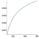
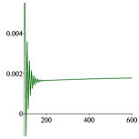
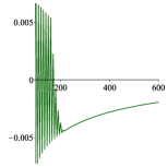
Figure 4. $\Delta_{n,M}^{(c)}-\Delta_{n,M}^{(v)}$ in the case of $\phi(z)=z+\frac{1}{2}z^{2}$: $100\leqslant n\leqslant 200$ (with step 5) and $M=0,1,2,3$ (in left to right order). Here $\Delta_{n,M}^{(\cdot)}$ is defined as in (19) but with $\frac{n^{M+1}}{(\log n)^{M+1}}$ there replaced by $n^{M+1}$.

In summary, we clarified here the often unclear situation of which version of the saddle-point contour to choose, and provided concrete examples for a more detailed comparison, from both analytic and numerical viewpoints. Such a clarification will be of instructional value, in addition to its own methodological interests.

3. A Lagrangean framework

Consider now the Lagrangean form

$$[z^{n}]f(z)\quad\text{with}\quad f=zG(f),$$

where $G(0)>0$. By Lagrange inversion relation, the Taylor coefficients satisfy

$$n[z^{n}]f(z)=[t^{n-1}]G(t)^{n}\qquad(n\geqslant 1).$$ (20)

This is one of the rare classes of functions for which both the singularity analysis and the saddle-point method apply well (see [9, p. 590] and [13]) because of (20). Under the following sub-criticality conditions:

$$\left\{\begin{split}&\bullet\text{$G$ is analytic in $|z|<\rho$, $0<\rho<\infty$;}\\ &\bullet\text{$[z^{j}]G(z)\geqslant 0$ and $\gcd\{j\,:\,[z^{j}]G(z)>0\}=1$;}\\ &\bullet\text{the equation $zG^{\prime}(z)=G(z)$ has a unique positive solution $\rho_{0}\in(0,\rho)$}\end{split}\right.$$ (21)

it is proved in [13] via singularity analysis that

$$[z^{n}]f(z)\sim\sum_{k\geqslant 0}c_{k}\binom{n-k-\frac{3}{2}}{n},\quad\text{with}\quad c_{k}=\frac{(-1)^{k}}{k}[t^{k-1}]\biggl{(}{\frac{1-\frac{(\rho+t)G(\rho)}{\rho G(\rho+t)}}{t^{2}}}\biggr{)}^{-\frac{1}{2}k},$$

where $\rho:=\frac{r}{G(r)}$ with $r>0$ solving the equation $rG^{\prime}(r)=G(r)$.

Here we examine this framework from the saddle-point method viewpoint. It turns out that the two asymptotic expressions we obtained above via two different contours are the same in this framework, and they are related to each other by a direct change of variables.

Theorem 3.1.

Write $\phi(z)=\log G(z)$.  Under the subcriticality conditions (21),

$$n[z^{n}]f(z)\sim\frac{R^{1-n}G(R)^{n}}{\sqrt{2\pi n}\,\sigma(R)}\sum_{m\geqslant 0}h_{2m}\frac{(-1)^{m}(2m)!}{2^{m}m!}\,(\sigma(R)^{2}n)^{-m},$$ (22)

where $R>0$ solves the equation $R\phi^{\prime}(R)=1$, $\sigma(R)^{2}=R\phi^{\prime}(R)+R^{2}\phi^{\prime\prime}(R)$ and

$$h_{m}=[v^{m}]\biggl{(}{\frac{\frac{1}{2}\sigma(R)^{2}v^{2}}{\phi(R(1+v))-\phi(R)-R\phi^{\prime}(R)\log(1+v)}}\biggr{)}^{\frac{1}{2}(m+1)}.$$ (23)

The expression for the coefficients in the expansion (22) is much simpler than that given in [13, Theorem 2].

Proof.

We work out the asymptotic expansion in the circular case, the vertical line case then following from a change of variables. As an asymptotic expansion of the form (22) can either be justified by singularity analysis as in [13] or by standard saddle-point analysis as in [7], we focus here on the (formal) calculation of the coefficients. By (20)

$$n[z^{n}]f(z) =\frac{1}{2\pi i}\oint_{|z|=r}z^{-n}G(z)^{n}{\,\rm d}z$$

$$=\frac{r^{1-n}}{2\pi i}\int_{-\pi i}^{\pi i}e^{u}(e^{-u}G(re^{u}))^{n}{\,\rm d}u$$

$$\thickapprox\frac{r^{1-n}G(r)^{n}}{2\pi\sigma(r)}\int_{-\varepsilon i}^{\varepsilon i}e^{\frac{1}{2}nv^{2}}g(v){\,\rm d}v,$$

where $\sigma(r)^{2}:=r\phi^{\prime}(r)+r^{2}\phi^{\prime\prime}(r)$, $r\phi^{\prime}(r)=1$, $g(v)=e^{u}\frac{{\,\rm d}u}{{\,\rm d}v}=\frac{{\,\rm d}}{{\,\rm d}v}e^{u}$, and

$$\frac{\phi(re^{u})-\phi(r)-r\phi^{\prime}(r)u}{\sigma(r)^{2}}=\frac{v^{2}}{2}.$$

We then deduce that

$$n[z^{n}]f(z)\sim\frac{r^{1-n}G(r)^{n}}{\sqrt{2\pi n}\,\sigma(r)}\sum_{m\geqslant 0}g_{2m}\frac{(-1)^{m}(2m)!}{2^{m}m!}\,(\sigma(r)^{2}n)^{-m},$$ (24)

where

$$g_{m}=[t^{m}]e^{t}\biggl{(}{\frac{\frac{1}{2}\sigma(r)^{2}t^{2}}{\phi(re^{t})-\phi(r)-r\phi^{\prime}(r)t}}\biggr{)}^{\frac{1}{2}(m+1)}.$$ (25)

By the change of variables $v=e^{t}-1$, we obtain the expression (23), which can also be obtained directly by beginning with the coefficient integral with the change of variables $z=R(1+v)$. ∎

In particular, if $\phi(z)=z$ or $G(z)=e^{z}$, then

$$n[z^{n}]f(z)=\frac{n^{n-1}}{(n-1)!}=[z^{n-1}]e^{nz},$$

and we obtain the same expressions as derived above for Stirling’s formula.

3.1. Catalan numbers

For simplicity, we consider only Catalan numbers for which $G(z)=(1-z)^{-1}$ or $\phi(z)=-\log(1-z)$, so that

$$[z^{n}]f(z)=[z^{n}]\frac{1-\sqrt{1-4z}}{2}=\frac{1}{n}\binom{2n-2}{n-1}.$$

Then the positive solution of the equation $r\phi^{\prime}(r)=1$ is given by $r=\frac{1}{2}$, and from either of the two equations (23) and (23), we have the asymptotic expansion ($\sigma(R)^{2}=2$)

$$\frac{1}{n}\binom{2n-2}{n-1}\sim\frac{4^{n-1}}{\sqrt{\pi}}\,\sum_{m\geqslant 0}h_{2m}\frac{(-1)^{m}(2m)!}{4^{m}m!}\,n^{-m-\frac{3}{2}},$$

and the identity

$$h_{m}:=[y^{m}]\biggl{(}{\frac{y^{2}}{-\log(1-y^{2})}}\biggr{)}^{\frac{1}{2}(m+1)}=[v^{m}]e^{v}\biggl{(}{\frac{v^{2}}{-\log(2-e^{v})-v}}\biggr{)}^{\frac{1}{2}(m+1)},$$

for $m\geqslant 0$, which follows simply by the change of variables $y=e^{v}-1$. Note particularly that $h_{2l+1}=0$ for $l\geqslant 0$.

On the other hand, by singularity analysis (see [9])

$$\frac{1}{n}\binom{2n-2}{n-1} =[z^{n}]\frac{1-\sqrt{1-4z}}{2}=-\frac{4^{n}}{4\pi i}\int e^{nt}\sqrt{1-e^{-t}}{\,\rm d}t$$

$$\sim-\frac{4^{n}}{4\pi i}\sum_{m\geqslant 0}b_{m}\int_{\mathcal{H}}e^{nt}t^{m+\frac{1}{2}}{\,\rm d}t\sim-\frac{4^{n}}{2}\sum_{m\geqslant 0}\frac{b_{m}}{\Gamma(-m-\frac{1}{2})}\,n^{-m-\frac{3}{2}},$$

where $b_{m}=[t^{m}]\bigl{(}{(1-e^{-t})/t}\bigr{)}^{\frac{1}{2}}$. Now by the relation

$$-\frac{1}{\Gamma(-m-\frac{1}{2})}=\frac{(-1)^{m}(2m+2)!}{\sqrt{\pi}(m+1)!4^{m+1}},$$

we then get

$$\frac{1}{n}\binom{2n-2}{n-1}\sim\frac{4^{n}}{2\sqrt{\pi}}\sum_{m\geqslant 0}\frac{b_{m}(-1)^{m}(2m+2)!}{(m+1)!4^{m+1}}\,n^{-m-\frac{3}{2}}.$$ (26)

It follows that $h_{2m}=(2m+1)b_{m}$, which can also be proved directly by a change of variables.

For large $m$, it is known (see [19, p. 39]) that

$$b_{m}\sim\frac{\sin(\frac{1}{2}m\pi)}{\sqrt{\pi}}\,(2\pi)^{-n}m^{-\frac{3}{2}},$$

implying that the expansion (26) is divergent for $n\geqslant 1$. Since the right-hand side is zero when $m$ is even, we can refine the approximation by the same singularity analysis and obtain

$$b_{m}\sim(-1)^{\lfloor{\frac{1}{2}m}\rfloor}(2\pi)^{-m}\times\begin{cases}\frac{3\sqrt{\pi}}{4}\,m^{-\frac{5}{2}},&\text{if $m$ is even};\\ \frac{1}{\sqrt{\pi}}\,m^{-\frac{3}{2}},&\text{if $m$ is odd}.\end{cases}$$

On the other hand, we can improve the asymptotic expansion by noting that

$$\biggl{(}{\frac{1-e^{-t}}{t}}\biggr{)}^{\frac{1}{2}}=e^{-\frac{1}{4}t}\Bigl{(}{\frac{2}{t}\sinh\frac{t}{2}}\Bigr{)}^{\frac{1}{2}}=e^{-\frac{1}{4}t}\sum_{m\geqslant 0}b_{2m}^{\prime}t^{2m};$$

thus, by the same singularity analysis

$$\frac{1}{n}\binom{2n-2}{n-1}\sim\frac{4^{n}}{2\sqrt{\pi}}\sum_{m\geqslant 0}\frac{b_{2m}^{\prime}(4m+2)!}{(2m+1)!4^{2m+1}}\,\bigl{(}{n-\tfrac{1}{4}}\bigr{)}^{-2m-\frac{3}{2}},$$

an expansion containing only even terms.

Yet another way to derive an asymptotic expansion for Catalan numbers is as follows. Let $G(z)=(1+z)^{2}$. Then

$$\frac{1}{n+1}\binom{2n}{n}=\frac{1}{n}[t^{n-1}](1+z)^{2n},$$

and we have

$$\frac{1}{n+1}\binom{2n}{n}\sim\frac{4^{n}}{\sqrt{\pi}}\sum_{m\geqslant 0}h_{2m}\frac{(-1)^{m}(2m)!}{m!}\,n^{-m-\frac{3}{2}},$$

where

$$h_{m}:=[v^{m}]\biggl{(}{\frac{v^{2}}{4\log\frac{(1+\frac{1}{2}v)^{2}}{1+v}}}\biggr{)}^{\frac{1}{2}{(m+1)}}.$$

By a direct change of variables, we have

$$h_{2m}=4^{-m}[y^{m}](2e^{y}-1)\sqrt{\frac{y}{1-e^{-y}}}.$$

References

- [1] J. M. Borwein and R. M. Corless. Gamma and factorial in the monthly. The American Mathematical Monthly, 125(5):400–424, 2018.
- [2] W. C. Boyd. Gamma function asymptotics by an extension of the method of steepest descents. Proceedings of the Royal Society of London. Series A: Mathematical and Physical Sciences, 447(1931):609–630, 1994.
- [3] S. Brassesco and M. A. Méndez. The asymptotic expansion for and the Lagrange inversion formula. The Ramanujan Journal, 24(2):219–234, 2011.
- [4] R. M. Corless and L. Rafiee Sevyeri. Stirling’s original asymptotic series from a formula like one of Binet’s and its evaluation by sequence acceleration. Experimental Mathematics, pages 1–8, 2019.
- [5] N. G. de Bruijn. Asymptotic methods in analysis. Dover Publications Inc., New York, third edition, 1981.
- [6] R. B. Dingle. Asymptotic expansions: their derivation and interpretation. Academic Press, 1973.
- [7] M. Drmota. A bivariate asymptotic expansion of coefficients of powers of generating functions. European Journal of Combinatorics, 15(2):139–152, 1994.
- [8] A. Erdélyi, W. Magnus, F. Oberhettinger, and F. Tricomi. Higher transcendental functions. Vol. I. McGraw-Hill (New York), 1953.
- [9] P. Flajolet and R. Sedgewick. Analytic combinatorics. Cambridge University Press, Cambridge, 2009.
- [10] B. Harris and L. Schoenfeld. The number of idempotent elements in symmetric semigroups. Journal of Combinatorial Theory, 3(2):122–135, 1967.
- [11] B. Harris and L. Schoenfeld. Asymptotic expansions for the coefficients of analytic functions. Illinois Journal of Mathematics, 12(2):264–277, 1968.
- [12] W. K. Hayman. A generalisation of Stirling’s formula. Journal für die reine und angewandte Mathematik, 196:67–95, 1956.
- [13] H.-K. Hwang, M. Kang, and G.-H. Duh. Asymptotic expansions for sub-critical lagrangean forms. In 29th International Conference on Probabilistic, Combinatorial and Asymptotic Methods for the Analysis of Algorithms (AofA 2018), pages 29:1–29–13. Schloss Dagstuhl-Leibniz-Zentrum fuer Informatik, 2018.
- [14] D. E. Knuth. The art of computer programming. Vol. 4A. Combinatorial algorithms. Part 1. Addison-Wesley, Upper Saddle River, NJ, 2011.
- [15] C. Mortici. The asymptotic series of the generalized Stirling formula. Computers & Mathematics with Applications, 60(3):786–791, 2010.
- [16] L. Moser and M. Wyman. An asymptotic formula for the Bell numbers. Trans. Roy. Soc. Canada Sect. III, 49:49–54, 1955.
- [17] L. Moser and M. Wyman. Asymptotic expansions II. Canadian Journal of Mathematics, 9:194–209, 1957.
- [18] G. Nemes. The role of resurgence in the theory of asymptotic expansions. PhD thesis, Central European University Budapest, Hungary, 2015.
- [19] N. E. Nørlund. Sur les valeurs asymptotiques des nombres et des polynômes de Bernoulli. Rendiconti del Circolo Matematico di Palermo, 10(1):27–44, 1961.
- [20] A. M. Odlyzko. Asymptotic enumeration methods. Handbook of combinatorics, 2(1063):1229, 1995.
- [21] A. M. Odlyzko and L. B. Richmond. Asymptotic expansions for the coefficients of analytic generating functions. Aequationes Mathematicae, 28(1):50–63, 1985.
- [22] OEIS Foundation Inc. The On-Line Encyclopedia of Integer Sequences.
- [23] R. Paris. On the asymptotic expansion of , Lagrange’s inversion theorem and the Stirling coefficients. arXiv preprint arXiv:1405.3423, 2014.
- [24] V. N. Sachkov. Combinatorial methods in discrete mathematics. Cambridge University Press, 1996.
- [25] G. Szekeres and F. E. Binet. On Borel fields over finite sets. Ann. Math. Statist., 28:494–498, 1957.
- [26] N. M. Temme. Special functions: An introduction to the classical functions of mathematical physics. John Wiley & Sons, 1996.
- [27] E. T. Whittaker and G. N. Watson. A course of modern analysis. Cambridge University Press, Cambridge, fourth edition, 1927.
- [28] R. Wong. Asymptotic approximations of integrals. SIAM, 2001.
- [29] M. Wyman. The asymptotic behaviour of the Laurent coefficients. Canadian Journal of Mathematics, 11:534–555, 1959.