A Pareto-optimal compositional energy-based model for sampling and optimization of protein sequences

Abstract

Deep generative models have emerged as a popular machine learning-based approach for inverse design problems in the life sciences. However, these problems often require sampling new designs that satisfy multiple properties of interest in addition to learning the data distribution. This multi-objective optimization becomes more challenging when properties are independent or orthogonal to each other. In this work, we propose a Pareto-compositional energy-based model (pcEBM), a framework that uses multiple gradient descent for sampling new designs that adhere to various constraints in optimizing distinct properties. We demonstrate its ability to learn non-convex Pareto fronts and generate sequences that simultaneously satisfy multiple desired properties across a series of real-world antibody design tasks.

1 Introduction

Generative models have shown promise across various applications in the life sciences for generating chemically- and physically-plausible designs and in accelerating the process of scientific discovery. Part of this trend of adoption can be owed to the convincing examples created by generative adversarial networks (GANs) [13], variational autoencoders (VAEs) [23], energy-based models (EBMs) [8] and, more recently, diffusion models [35; 32; 5]. However, there are far fewer success stories in real-world industry applications [6; 15]. Some reasons include an overrepresenation of image datasets; a lack of evaluation protocols and metrics for synthetic data [37; 33]; challenges around controllable generation and training — for exmaple GANs; and challenges in generating samples that are different from have been seen during training [22; 2; 38]. Taken together, these serve to limit the applicability of generative modeling for real-world use cases.

Our work is motivated by this and, in particular, the need to accelerate the development and discovery of new molecules, namely therapeutic antibodies. Though several generative models have already been proposed for these purposes [10; 12; 31], generating new samples without guidance or control does not guarantee downstream success of the proposed molecules. In practice, each molecule has to satisfy multiple properties. For therapeutic antibodies, this could include properties such as binding affinity, polyreactivity, and viscosity [1; 20; 39]. Failure to account for these and other properties can lead to serious complications later on during scale-up, manufacturing, and clinical trials and the optimization of straightforward objectives does not necessarily translate into progress in the laboratory [28].

Motivated by this challenge, we propose a new EBM for antibody design that simultaneously takes into account multiple properties that an antibody has to satisfy. The adherence to multiple properties is a challenge in itself, as it often involves optimizing multiple conflicting objectives. In antibodies, for instance, optimization of binding affinity alone may come at the expense of developability properties, parameters that govern the likelihood of success of a molecule during manufacturing and quality control .

In general, in optimizing multiple conflicting properties, it is often impossible to find a single sample that satisfies all of the objectives simultaneously [21]. We argue that, instead, one should aim to propose a set of diverse data points from the Pareto front [3] that correspond to different choices for various objective functions. Doing so enables a global perspective the optimal trade-off between objectives and can select a molecule according to their preference. To achieve Pareto optimality, we rely on recent advances in multi-objective optimization (MOO)[34; 27] as well as on compositional sampling with EBMs [8] to build a Pareto-optimal compositional EBM (pcEBM). Figure 1 exemplifies both why we need pcEBM and what we achieve with it when optimizing a design of an initial antibody sequence.

We first present the the necessary background on multi-objective optimization in subsection 2.1 and related work on compositional sampling with EBM in subsection 2.2 leading to pcEBM described in subsection 2.3. In section 3 we include empirical evaluation and discussion, before concluding in section 4.

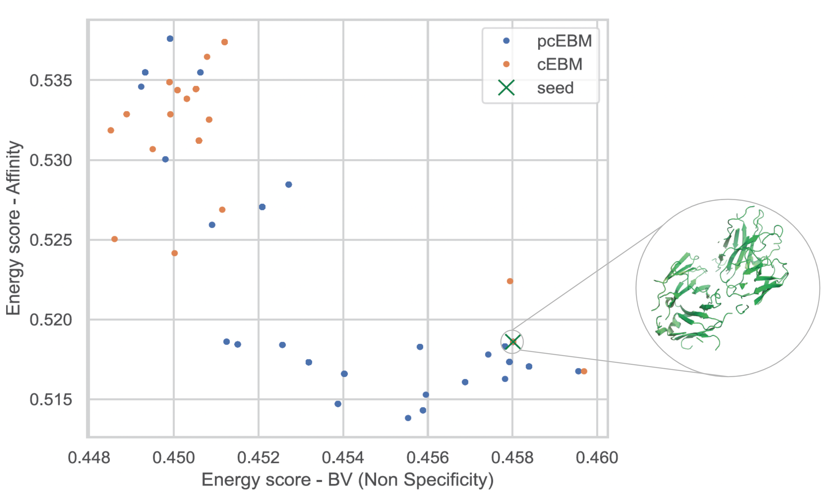
Figure 1: Example output of the proposed Pareto-optimal energy-based sampler (pcEBM) compared to a naive multi-objective sampling (cEBM). The green marker denotes the starting sequence; each point in the plot corresponds to a modified design of that starting point, aiming at improving affinity and nonspecificity (BV-ELISA or BV score). pcEBM introduces samples along a Pareto front, with candidates minimizing both objectives simultaneously, while candidates generated by the cEBM minimize only one objective.

2 Background and method

Problem setup. Antibodies are composed of two chains of amino acids (AA), which can be represented as sequences of characters. Each AA comes from an alphabet of 20 characters corresponding , typically of combined length $L\sim 250$. We will denote the sequences as $\mathbf{}{x}=(x_{1},\ldots,x_{L})$, where $x_{l}\in\{1,\ldots,20\}$ corresponds to the AA type at position $l$. For each of those sequences, we measure $m$ properties, such that $f_{i}:\mathbb{R}^{L}\rightarrow\mathbb{R}$ for all $i\in 1,\ldots,m$.

Our goal is to generate new sequences $x^{*}$ with preferred values for each of the $m$ properties. Since we cannot fully satisfy all of the properties/objectives simultaneously (they may be conflicting with each other), we are interested in finding samples which can not be further improved simultaneously for all the objectives, yielding the notion of Pareto optimality [4].

Definition 2.1 (Pareto Optimality [4; 27])

For $x_{1},x_{2}\in\mathbb{R}^{d}$, we say that $x_{1}$ is dominated by $x_{2}$ iff $f_{i}(x_{2})\leq f_{i}(x_{1}),\forall i\in[m]$. A point $x^{*}$ is called globally Pareto optimal on $\mathbb{R}^{d}$ iff it is not dominated by any other $x^{\prime}\in\mathbb{R}^{d}$. A point $x*$ is called locally Pareto optimal iff there exists an open neighborhood $\mathcal{N}(x^{*})$ of $x^{*}$, such that $x^{*}$ is not dominated by any $x\in\mathcal{N}(x^{*})$. The collection of globally (resp. locally) Pareto optimal points are called the global (resp. local) Pareto set. The collection of function values $F(x^{*})=(f_{1}(x^{*}),f_{2}(x^{*}),\dots,f_{m}(x^{*}))$ of all the Pareto points $x^{*}$ is called the Pareto front.

2.1 Multi-objective optimization

A simple approach to solving MOO is linear scalarization [21] based on a preference vector $\lambda=[\lambda_{1},\ldots,\lambda_{m}]$ from the probability simplex on $[m]$, i.e., $S=\{\lambda:\sum_{i=1}^{m}\lambda_{i}=1,\lambda_{i}\geq 0,i\in[m]\}$. Each $\lambda\in S$ leads to a weighted objective function $f_{\lambda}(x)=\sum_{i=1}^{m}\lambda_{i}f_{i}(x)$ and its minimizer $x^{*}_{\lambda}=\text{argmin}_{x}f_{\lambda}(x)$. As we evaluate on $\lambda$ from a grid of $S$, we hope that the corresponding $x^{*}_{\lambda}$ approximates the Pareto front. The solutions obtained by linear scalarization lie in the convex envelope of the Pareto front, which renders the approach plausible for situations where the Pareto front is convex [27].

An alternative approach for non-convex Pareto fronts is multiple gradient descent (MGD) [7], which iteratively updates variable $x$ along a direction that ensures that all objectives are decreased simultaneously and guides the optimization towards a Pareto improvement. Denote the gradient of the $i$-th objective as $\nabla_{x}f_{i}(x)$. With gradient descent, we update the variable $x^{k}\leftarrow x^{k-1}-\eta g(x)$, where $g(x)$ is a vector to be determined and $\eta$ is a small step size. From a 1st-order Taylor expansion, we can deduce that $\langle\nabla_{x}f_{i}(x),g\rangle\approx-(f_{i}(x^{k})-f_{i}(x^{k-1}))/\eta$ which represents the decreasing rate of $f_{i}$ when we update $x$ along direction $g(x)$. In MGD, $g$ is chosen to maximize the slowest decreasing rate among all the objectives, that is:

$$g(x)\propto\operatorname*{argmax}_{g\in\mathbb{R}^{d}}\{\min_{i\in[m]}\langle g,\nabla_{x}f_{i}(x)\rangle\ \text{subject to}\ \|g\|_{2}\leq 1\}$$ (1)

By doing so, $g(x)$ is pushed to have positive inner products with all $\nabla_{x}f_{i}(x)$. If the latter is impossible, $\{\nabla_{x}f_{i}(x)\}_{i=1}^{m}$ will contain conflicting directions and we will get $g(x)=0$ which terminates the procedure. By using Lagrangian duality, Désidéri [7] has shown that the above objective has the optimal value $g(x)\approx\sum_{i=1}^{m}\lambda_{i}^{*}\nabla_{x}f_{i}(x)$ where $\{\lambda_{i}\nabla_{x}f_{i}(x)\}_{i=1^{m}}$ is the solution of

$$\min_{\lambda_{i}}\|\sum_{i=1}^{m}\lambda_{i}\,\nabla_{x}f_{i}(x)\|_{2}\ \text{subject to}\ \sum_{i=1}^{m}\lambda_{i}=1\ \text{and}\ \lambda_{i}\geq 0\ \text{for all}\ i\in[m].$$

The above convex optimisation problem has a closed form solution when $m=2$ and a fast algorithm for $m>2$ [34; 19]. By construction, when the step size is small, MGD decreases monotonically all objectives simultaneously and will terminate at a local Pareto point.

2.2 Compositional energy-based models

Although EBMs have been around for many years [25; 24], recent interest in generative modeling has led to a resurgence of interest [8; 9]. EBMs learn to represent data by approximating an unnormalized probability distribution across data. They do so by learning an energy function $E_{\theta}(x)$ parameterized by a neural network that maps each input $x$ to a scalar real value interpreted as the energy and approximating the data distribution by the Boltzmann distribution under unit temperature:

$$p_{\theta}(x)\propto e^{-E_{\theta}(x)}.$$

Training an EBM on a given data distribution is usually done by contrastive divergence [16]. Besides predicting the un-normalized data likelihood, EBMs can be used to sample new data points $x$ from $p_{\theta}$ (during both training and generation). Sampling is typically performed by some Markov-Chain Monte-Carlo (MCMC) procedure. We consider the common case of Langevin Diffusion (LD) where the samples are initialized from refinement/uniform random noise followed by iterative refinement:

$$x=x^{k-1}-\frac{\eta}{2}\nabla_{x}E_{\theta}(x^{k-1})+\omega^{k},\ \omega\sim\mathcal{N}(0,\sigma^{2}),$$ (2)

with $k$ being the sampling step and $\eta$ the step size.

The above sampling procedure can be easily extended to produce samples from the composition of $p_{\theta}$ with other distributions of interest. Along this direction, Du et al. [9] considered the problem of sampling from $m$ composed distributions, each modeling a different propertiey $f_{i}$, an approach referred to as compositional EBM (cEBM). Du et al. proposed multiple variations for executing different logical operations over properties of interest, such as conjunction, negation, and disjunction. In the following, we focus on conjunction, which corresponds to combining individual EBMs as a product of experts:

$$p(x|f_{1}\wedge f_{2}\wedge\cdots\wedge f_{m})=\prod_{i}p(x|f_{i})\propto e^{-\sum_{i}E(x|f_{i})}.$$

We also note that cEBM utilized the following sampling procedure:

$$x=x^{k-1}-\frac{\eta}{2}\nabla_{x}\sum_{i}E_{\theta}(x^{k-1}|f_{i})+\omega^{k},\ \omega\sim\mathcal{N}(0,\sigma^{2}),$$ (3)

which amounts to applying LD w.r.t. $E(x)=\sum_{i}E(x|f_{i})$.

2.3 Pareto compositional sampling

Inspired by previous work on multi-objective optimization [7; 27] discussed in subsection 2.1, we here propose pcEBM, a method that samples from the Pareto front of $m$ Boltzmann distributions of interest. Our approach entails utilizing multiple gradient descent to select a locally optimal direction that optimizes the slowest decreasing rate among all the objectives of the compositional EBMs:

$$x^{k}\leftarrow x^{k-1}-\eta\operatorname*{argmax}_{g\in\mathbb{R}^{d}}\{\min_{i\in[m]}\langle g,\nabla_{x}f_{i}(x^{k-1})\rangle\ \text{subject to}\ \|g\|_{2}\leq 1\}+\sqrt{2}\alpha\omega,$$ (4)

where $\alpha$ is a positive constant and the internal optimization problem is the same utilized in MGD and the external sampler is performing Langevin diffusion.

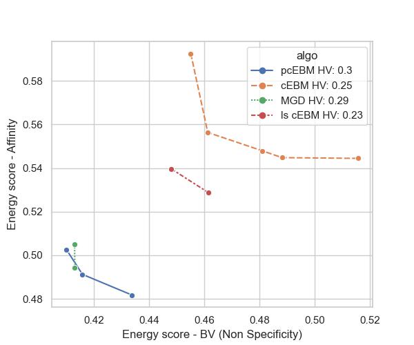
Figure 2: Pareto fronts and estimated hyper volume for all baselines with $\eta=0.01$ and $k=400$. The axes show the energy of EBMs that were separately trained on data with good affinity and BV scores, respectively, with smaller energies being more desirable.

Suppose that we are generating a new sequence $x$, either by starting from random noise or by improving an existing one. At each step $k$, if $x^{k-1}$ is far from the Pareto front and the gradients $\nabla_{x}f_{i}(x^{k-1})$ have non-negligible norm, Equation 4 will drive $x^{k-1}$ closer to the Pareto front. On the other hand, when $x^{*}$ is close to the Pareto front and the gradients have nearly vanished, the noise dominates and $x^{k-1}$ performs Brownian motion. As will be demonstrated experimentally, the addition of noise $\omega$ helps pcEBM to explore more efficiently the Pareto as compared to MGD, whereas the locally optimal determination of the optimization direction renders the optimization more effective than cEBM.

3 Empirical evaluation

In the following, we compare the Pareto compositional EBM pcEBM with three baselines: multiple gradient descent (MGD) [7], a compositional EBM (cEBM) [9], and a linearly scaled cEBM (ls-cEBM) [21].

Experimental setup. We wish to generate plausible antibody sequences according to three key properties: (i) similarity to known human antibodies from the public database of observed antibodies [29] (Ab-like), (ii) binding affinity to antigens of interest (Aff), and (iii) an experimental measure of nonspecificity — phenomena which can affect the dosing regimen, safety, and overall therapeutic profile of an antibody — which we refer to as the BV score  [17] . We use datasets from both public and proprietary sources to train three separate EBMs, each pertaining to a property of interest. Though alternative choices are also possible, we instantiate all models as sequence-based convolution networks [11]. More details on the architecture can be found in the Appendix. We use the same models for sampling new sequences with each of the baselines. The differences in implementation are as follows: MGD does not add any noise, cEBM uses Lanvegin dynamics but has uniform weights for all properties; ls-cEBM differs from cEBM in that it includes domain-informed weights; and finally pcEBM learns the optimal weights for each property per sequence. Each baseline relies on two main hyper-parameters, namely the step size $\eta$ and the number of steps $k$.

To compare different approaches in terms of their ability to satisfy multiple properties, we adopt the Hyper-Volume (HV) metric from the multi-objective optimization literature [14] computed over the energy scores of each property model. In all experiments, we aim for minimizing the energy scores per property. Additionally, as a proxy for how well the sampled sequences capture the properties of interest we compute the minimal edit distance of each sampled sequence to the ones seen during the training of each property EBM ($e_{dist}$) [30]. More details about the computation of these metrics can be found in the Appendix.

Results and discussion. Our experiments are designed to provide answers to the following research questions:

• Q.1 Can we use EBMs to generate valid/reasonable, multi-property compliant antibody sequences?

• Q.2 Does sampling with Langevin Dynamics propose more Pareto optimal sequences?

• Q.3 Does pcEBM have an advantage over cEBM?

• Q.4 Starting from a seed sequence, can we improve a property of interest using (p)cEBM?

	HV(Ab-Like, Aff, BV)	HV(Aff, BV)	HV(Ab-Like, BV)	HV(Ab-Like, Aff)
$\eta=0.01$
MGD	0.04	0.22	0.23	0.29
ls-cEBM	0.00	0.24	0.24	0.23
cEBM	0.00	0.25	0.24	0.25
pcEBM	0.049	0.3	0.29	0.30
$\eta=1$
MGD	0.04	0.25	0.25	0.27
ls-cEBM	0.00	0.25	0.24	0.25
cEBM	0.046	0.29	0.29	0.3
pcEBM	0.041	0.27	0.27	0.29
$\eta=40$
MGD	0.033	0.25	0.25	0.26
ls-cEBM	0.043	0.27	0.26	0.26
cEBM	0.046	0.29	0.29	0.29
pcEBM	0.037	0.27	0.27	0.28

Table 1: Hyper-Volume (HV) across multiple combinations of properties (as measured by energy score) across different step sizes $\eta$. Larger scores indicate bigger improvement. The best results for are typeset in boldface.

	$e_{dist}$(generated, Ab-like)	$e_{dist}$(generated, BV)	$e_{dist}$(generated, Aff)	average $e_{dist}$
single-property EBM
Ab-Like EBM	98.74 ($\pm$19.25)	93.84 ($\pm$19.05)	103.3 ($\pm$17.8)	98.62
Stc EBM	84.68 ($\pm$15.78)	69.7 ($\pm$ 16.42)	88.29 ($\pm$ 5.72)	121.33
Aff EBM	88.51 ($\pm$16.25)	81.4 ($\pm$15.6)	86.73 ($\pm$6.31)	85.55
$\eta=40$
MGD	83.51 ($\pm$16.1)	71.49 ($\pm$15.7)	85.84 ($\pm$16.3)	80.28
cEBM	92.96 ($\pm$ 19.03)	86.86 ($\pm$ 17.99)	97.97 ($\pm$ 17.28)	92.60
ls-cEBM	92.4 ($\pm$ 19.3)	87.14 ($\pm$ 17.94)	97.93 ($\pm$ 17.25)	92.49
pcEBM	82.24 ($\pm$16.16)	71.47 ($\pm$ 15.82)	85.76 ($\pm$ 16.34)	79.82
$\eta=0.01$
MGD	91.46 ($\pm$16.23)	84.02 ($\pm$15.43)	92.91 ($\pm$16.48)	89.46
cEBM	219.23 ($\pm$4.43)	222.47 ($\pm$ 4.45)	221.99 ($\pm$ 4.4)	221.23
ls-cEBM	218.78 ($\pm$4.66)	218.13 ($\pm$4.58)	218.62 ($\pm$4.73)	218.51
pcEBM	89.35 ($\pm$ 14.64)	79.67 ($\pm$ 13.99)	89.04 ($\pm$ 14.37)	86.02

Table 2: Edit distance (mean with standard deviation in brackets) to sequences in the training set with property of interest. Results in bold are best per columns, smaller is better, considering $e_{dist}$ as a proxy for similarity to real data with the specific property.

Table 1 and Table 2 address Q.1. We find that EBMs trained on data possessing a single property of interest propose sequences that are similar to those sharing the same property, but are dissimilar to the sequences preferred by other objectives. In contrast, sequences generated by a multi-property EBMs have smaller distances to all properties compared to the single-property EBMs. Amongst the four considered multi-objective baselines, pcEBM generates sequences with greater hyper-volume and similarity to the training datasets, whereas MGD is a close second.

We surmise the difference between cEBM and pcEBM is owed to their speed of convergence. We confirm this in Figure 3 by plotting the energy score at each sampling step for both cEBM and pcEBM with a step size of $\eta=0.01$. As observed, for the same starting sequence pcEBM converges faster. This result partially answers Q.3.

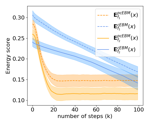
Figure 3: Energy scores per property $f_{i}$ at each step for pcEBM and cEBM; same sequence and same step size $\eta=0.01$.

To further test our approach, we calculate HV across the three properties we aim to account for. Here, we consider the energy of each property EBM as proxy for the objective of interest. The advantage of pcEBM is noticeable at smaller step sizes (see Table 1), while the variance in both edit distance and hyper-volume for different $\eta$ is significantly smaller for pcEBM than others. Figure 2 depicts the Pareto front for two properties obtained from candidate sequences from each baseline. We find that the pcEBM front is broader than MGD-based approaches, which agres our supposition that employing LD leads to an improved coverage of the Pareto front as compared to pure gradient descent. Further, pcEBM and MGD fronts are closer to the origin that that obtained by direct LD, which demonstrates the advantage of the multi-properly optimization aspect of pcEBM, addressing Q.2 and Q.3.

Finally, for Q.4 we wish to explore the possibility for improving properties of already existing antibodies by using the variants of compositional EBMs. We focus our analysis on nonspecificity (BV) as we have an external SeqCNN classifier that can act as a surrogate pseudo-oracle. We start by screening the existing sequences to select only those with low BV scores, which we refer to as “seeds”. We use sequences with poor experimental and predicted BV scores as seed sequences for generation and then reuse the nonspecificity pseudo-oracle to evaluate the newly proposed designs. Figure 5 shows the BV score improvement achieved by each baseline. We notice that the multi-objective methods manage to improve the worst BV scores from 0.27 to above 0.9, with MGD and pcEBM giving a slightly lower average score than cEBM (though all scores are comparably high).

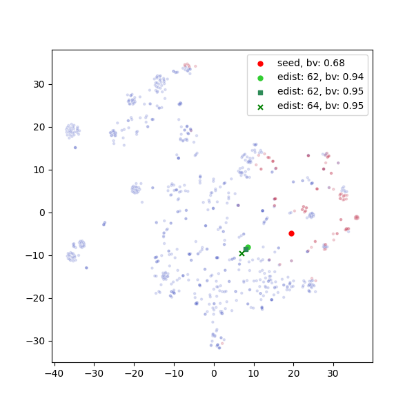
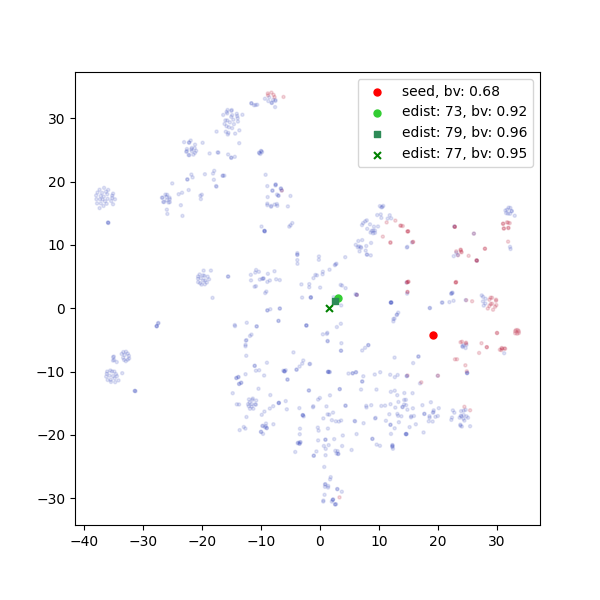
Figure 4: tSNE embeddings of antibody sequences colored based on BV score, with blue sequences having better scores. The figures show how a sequence with poor BV score of 0.68 (in orange) is improved by two models. Left - cEBM, Right - pcEBM.

The plots in Figure 4 provide further insight into the nonspecificity optimization process by examining a low-dimensional embedding of seed and optimized sequences. The embedding is obtained by using tSNE to project the last layer feature representations of the sequences obtained from the nonspecificity oracle, onto a 2D space. We color each point (sequence) by their BV score with blue indicating a good score and red a poor one. On the same plot, we overlay a seed sequence and its corresponding proposed designs. We see that both cEBM and pcEBM improve the probability for a good nonspecificity score, and move the seed towards the section of the manifold covered by datapoints with good scores.

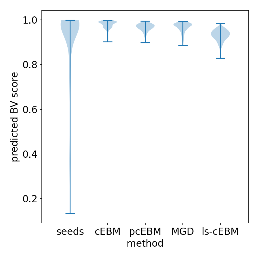
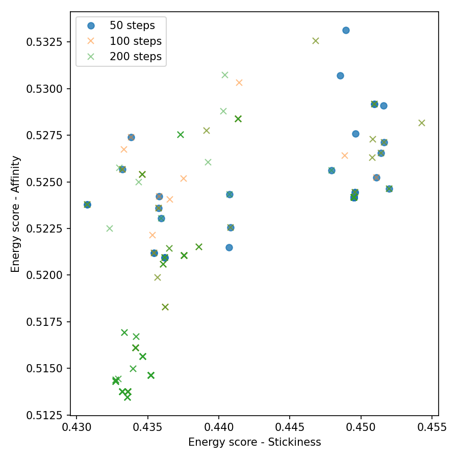
Figure 5: Left - violin plots of the distributions of predicted BV scores for the initial set of sequences to be improved (seeds), and for the proposed designs from each baseline. Higher BV scores are better. Right - energy scores of trajectories proposed by pcEBM for a different number of steps. Lower energy scores are better/preferred for the objectives.

4 Conclusion

We propose a new approach to sampling data points that simultaneously satisfy multiple desired properties. We do so by integrating multiple gradients within compositional energy based models. In a series of experiments for generating and improving existing sequences, we validate the performance of the compositional EBMs as well as their Pareto optimality. The generality and modularity of pcEBM allow for multiple expansions we are excited to explore: (i) other data types, in particular graph structures suitable for molecules, (ii) incorporating other sampling frameworks such as Stein variational gradient descent [26], (iii) incorporating uncertainty estimates, and (iv) Pareto-optimal training for EBMs, to name a few.

Appendix

4.1 Additional details on experiments

SeqCNNs

For all properties and baselines we use an identical NN architecture, that is one model per protein chain, consisted of three Conv1D layers with kernel size 9 and padding 1, ReLU non-linearities and penultimate layer of size 256. All EBMs were trained with contrastive training, Adam optimizer and early stopping criterion.

Hyperparameters

For each multipropery sampling baseline, the following hyper parameter grid was explored with random search:

• step size - $\eta\in\{1^{e-4},1^{e-2},1,10,40\}$

• number of steps - $k\in\{100,200,300,400\}$

• noise type - $\omega\in\{\mathcal{N},\mathcal{U}\}$.

4.2 Metrics

Hypervolume

HV is an indicator for evaluating the quality of sets of solutions in multi objective optimization. For a given reference point of $r=[r_{1},...,r_{m}]$ we have an upper bound of the objectives, such that $supxf_{i}(x)\leq r_{i},\forall i\in[m]$. For a given set of solutions $\mathcal{X}=\{x_{l}\}^{n}_{l=1}$, a hypervolume indicator $HV(\mathcal{X})$ is a measure of the region between all $f_{i}$ objectives and $r$:

$$HV(\mathcal{X})=\Lambda\{(q\in\mathbb{R}^{d}|\exists x\in\mathcal{X}:q\in\prod_{i}^{m}[f_{i}(x),r_{i}]\})$$

where $\Lambda(\cdot)$ denotes the Lebesgue measure.

In the context of our experiments, we are interested in minimizing the energy scores per each property, and we choose a reference point $r=(1.0,1.0,1.0)$. We compte HV from each Pareto front to the reference point with the implementation provided in PyMoo [18].

Edit distance

Edit distance is the typical score for quantifying how dissimilar two strings (in our case, sequences) are to one another, measured by counting the minimum number of operations required to transform one string into the other. Although different variants exist, here we rely on the Levenshtein distance which accounts for insertions, deletions and substitutions. In all experiments we use the python library edist as implemented in [36].

References

- Bailly et al. [2020] M. Bailly, C. Mieczkowski, V. Juan, E. Metwally, D. Tomazela, J. Baker, M. Uchida, E. Kofman, F. Raoufi, S. Motlagh, et al. Predicting antibody developability profiles through early stage discovery screening. In MAbs, volume 12, page 1743053. Taylor & Francis, 2020.
- Barz and Denzler [2020] B. Barz and J. Denzler. Do we train on test data? purging cifar of near-duplicates. Journal of Imaging, 6(6):41, 2020.
- Censor [1977] Y. Censor. Pareto optimality in multiobjective problems. Applied Mathematics and Optimization, 4(1):41–59, 1977.
- Chinchuluun and Pardalos [2007] A. Chinchuluun and P. M. Pardalos. A survey of recent developments in multiobjective optimization. Annals of Operations Research, 154(1):29–50, 2007.
- Conard [2022] J. Conard. How gpt-3 wrote a movie about a cockroach-ai love story. In Wired, 2022.
- Davis [2020] D. Davis. Generative design is doomed to fail. In Blog post, 2020.
- Désidéri [2012] J.-A. Désidéri. Multiple-gradient descent algorithm (mgda) for multiobjective optimization. Comptes Rendus Mathematique, 350(5-6):313–318, 2012.
- Du and Mordatch [2019] Y. Du and I. Mordatch. Implicit generation and modeling with energy based models. Advances in Neural Information Processing Systems, 32, 2019.
- Du et al. [2020] Y. Du, S. Li, and I. Mordatch. Compositional visual generation with energy based models. Advances in Neural Information Processing Systems, 33:6637–6647, 2020.
- Eguchi et al. [2022] R. R. Eguchi, C. A. Choe, and P.-S. Huang. Ig-vae: Generative modeling of protein structure by direct 3d coordinate generation. PLoS computational biology, 18(6):e1010271, 2022.
- Gehring et al. [2017] J. Gehring, M. Auli, D. Grangier, D. Yarats, and Y. N. Dauphin. Convolutional sequence to sequence learning. In International conference on machine learning, pages 1243–1252. PMLR, 2017.
- Gligorijevic et al. [2021] V. Gligorijevic, D. Berenberg, S. Ra, A. Watkins, S. Kelow, K. Cho, and R. Bonneau. Function-guided protein design by deep manifold sampling. bioRxiv, 2021.
- Goodfellow et al. [2020] I. Goodfellow, J. Pouget-Abadie, M. Mirza, B. Xu, D. Warde-Farley, S. Ozair, A. Courville, and Y. Bengio. Generative adversarial networks. Communications of the ACM, 63(11):139–144, 2020.
- Guerreiro et al. [2020] A. P. Guerreiro, C. M. Fonseca, and L. Paquete. The hypervolume indicator: Problems and algorithms. arXiv preprint arXiv:2005.00515, 2020.
- Hao [2022] R. Hao. Deep generative models could offer the most promising developments in ai. In Venture Beat, 2022.
- Hinton [2002] G. E. Hinton. Training products of experts by minimizing contrastive divergence. Neural computation, 14(8):1771–1800, 2002.
- Hötzel et al. [2012] I. Hötzel, F.-P. Theil, L. J. Bernstein, S. Prabhu, R. Deng, L. Quintana, J. Lutman, R. Sibia, P. Chan, D. Bumbaca, et al. A strategy for risk mitigation of antibodies with fast clearance. In MAbs, volume 4, pages 753–760. Taylor & Francis, 2012.
- J and K [2020] B. J and D. K. pymoo: Multi-objective optimization in python. IEEE Access, 8:89497–89509, 2020.
- Jaggi [2013] M. Jaggi. Revisiting frank-wolfe: Projection-free sparse convex optimization. In International Conference on Machine Learning, pages 427–435. PMLR, 2013.
- Jain et al. [2017] T. Jain, T. Sun, S. Durand, A. Hall, N. R. Houston, J. H. Nett, B. Sharkey, B. Bobrowicz, I. Caffry, Y. Yu, et al. Biophysical properties of the clinical-stage antibody landscape. Proceedings of the National Academy of Sciences, 114(5):944–949, 2017.
- Kaisa M. Miettinen [2003] S. Kaisa M. Miettinen, Sayin. Nonlinear multiobjective optimization. European Journal of Operational Research, 148(1):229–230, 2003.
- Karras et al. [2017] T. Karras, T. Aila, S. Laine, and J. Lehtinen. Progressive growing of gans for improved quality, stability, and variation. arXiv preprint arXiv:1710.10196, 2017.
- Kingma and Welling [2013] D. P. Kingma and M. Welling. Auto-encoding variational bayes. arXiv preprint arXiv:1312.6114, 2013.
- LeCun et al. [2006] Y. LeCun, S. Chopra, R. Hadsell, M. Ranzato, and F. Huang. A tutorial on energy-based learning. Predicting structured data, 1(0), 2006.
- LeCun et al. [2007] Y. LeCun, S. Chopra, M. Ranzato, and F.-J. Huang. Energy-based models in document recognition and computer vision. In Ninth International Conference on Document Analysis and Recognition (ICDAR 2007), volume 1, pages 337–341. IEEE, 2007.
- Liu [2017] Q. Liu. Stein variational gradient descent as gradient flow. Advances in neural information processing systems, 30, 2017.
- Liu et al. [2021] X. Liu, X. Tong, and Q. Liu. Profiling pareto front with multi-objective stein variational gradient descent. Advances in Neural Information Processing Systems, 34:14721–14733, 2021.
- Nigam et al. [2022] A. Nigam, R. Pollice, G. Tom, K. Jorner, L. A. Thiede, A. Kundaje, and A. Aspuru-Guzik. Tartarus: A benchmarking platform for realistic and practical inverse molecular design. arXiv preprint arXiv:2209.12487, 2022.
- Olsen et al. [2022] T. H. Olsen, F. Boyles, and C. M. Deane. Observed antibody space: A diverse database of cleaned, annotated, and translated unpaired and paired antibody sequences. Protein Science, 31(1):141–146, 2022.
- Paaßen et al. [2018] B. Paaßen, C. Gallicchio, A. Micheli, and B. Hammer. Tree edit distance learning via adaptive symbol embeddings. In International Conference on Machine Learning, pages 3976–3985. PMLR, 2018.
- Repecka et al. [2021] D. Repecka, V. Jauniskis, L. Karpus, E. Rembeza, I. Rokaitis, J. Zrimec, S. Poviloniene, A. Laurynenas, S. Viknander, W. Abuajwa, et al. Expanding functional protein sequence spaces using generative adversarial networks. Nature Machine Intelligence, 3(4):324–333, 2021.
- Roose [2022] K. Roose. We need to talk about how good a.i. is getting. In The New York Times, 2022.
- Sajjadi et al. [2018] M. Sajjadi, O. Bachem, M. Lucic, O. Bousquet, and S. Gelly. Assessing generative models via precision and recall. Advances in neural information processing systems, 31, 2018.
- Sener and Koltun [2018] O. Sener and V. Koltun. Multi-task learning as multi-objective optimization. Advances in neural information processing systems, 31, 2018.
- Sohl-Dickstein et al. [2015] J. Sohl-Dickstein, E. Weiss, N. Maheswaranathan, and S. Ganguli. Deep unsupervised learning using nonequilibrium thermodynamics. In International Conference on Machine Learning, pages 2256–2265. PMLR, 2015.
- Šošić and Šikić [2017] M. Šošić and M. Šikić. Edlib: a c/c++ library for fast, exact sequence alignment using edit distance. Bioinformatics, 33(9):1394–1395, 2017.
- Theis et al. [2015] L. Theis, A. v. d. Oord, and M. Bethge. A note on the evaluation of generative models. arXiv preprint arXiv:1511.01844, 2015.
- van den Burg and Williams [2021] G. van den Burg and C. Williams. On memorization in probabilistic deep generative models. Advances in Neural Information Processing Systems, 34:27916–27928, 2021.
- Wolf Pérez et al. [2022] A.-M. Wolf Pérez, N. Lorenzen, M. Vendruscolo, and P. Sormanni. Assessment of therapeutic antibody developability by combinations of in vitro and in silico methods. In Therapeutic Antibodies, pages 57–113. Springer, 2022.