On Learning Fairness and Accuracy on Multiple Subgroups

Abstract

We propose an analysis in fair learning that preserves the utility of the data while reducing prediction disparities under the criteria of group sufficiency. We focus on the scenario where the data contains multiple or even many subgroups, each with limited number of samples. As a result, we present a principled method for learning a fair predictor for all subgroups via formulating it as a bilevel objective. In the lower-level, the subgroup-specific predictors are learned through a small amount of data and the fair predictor. In the upper-level, the fair predictor is updated to be close to all subgroup specific predictors. We further prove that such a bilevel objective can effectively control the group sufficiency and generalization error. We evaluate the proposed framework on real-world datasets. Empirical evidence suggests the consistently improved fair predictions, as well as the comparable accuracy to the baselines.

1 Introduction

Machine learning has made rapid progress in sociotechnical systems such as automatic resume screening, video surveillance, and credit scoring for loan applications. Simultaneously, it has been observed that learning algorithms exhibited biased predictions on the subgroups of population [1, 2]. For example, the algorithm denies a loan application based on sensitive attributes such as gender, race, or disability, which has heightened public concerns.

To this end, fair learning is recently highlighted to mitigate prediction disparities. The high-level idea is quite straightforward: adding fair constraints during the training [3]. As a result, fair learning principally gives rise to two desiderata. On the one hand, the fair predictor should be informative to ensure accurate predictions for the data. On the other hand, the predictor is required to guarantee fairness to avoid prediction disparities across subgroups. Therefore, it is crucial to understand the possibilities and then design provable approaches for achieving both informative and fair learning.

Clearly, achieving both objectives depends on predefined fair notations. Consider demographic parity [1] as the fair criteria, which necessitates the independence between the predictor’s output $f(X)$ and the sensitive attribute (or subgourp index) $A$. Thus, if the sensitive attribute $A$ and the ground-truth label $Y$ are highly correlated, it is impossible to learn a both fair and informative predictor.

To avoid such intrinsic impossibilities, alternative fair notions have been developed. In this work, we focus on the criteria of group sufficiency [1, 4], which ensures that the conditional expectation of ground-truth label ($\mathbb{E}[Y|f(X),A]$) is identical across different subgroups, given the predictor’s output. Notably, the risk of violating group sufficiency has arisen in a number of real-world scenarios. E.g., in medical artificial intelligence, the machine learning algorithm is used to assess the clinic risk, and guide decisions regarding initiating medical therapy. However, [5, 6] revealed a significant racial bias in such algorithms: when the algorithm predicts the same clinical risk score $f(X)$ for white and black patients, black patients are actually at a higher risk of severe illness: $\mathbb{E}[Y|f(X),A=\text{black}]\gg\mathbb{E}[Y|f(X),A=\text{white}]$. The deployed algorithms have resulted in more referrals of white patients to specialty healthcare services, resulting in both spending disparities and racial bias [5].

In summary, this work aims to propose a novel principled framework for ensuring group sufficiency, as well as preserving an informative prediction with a small generalization error. In particular, we focus on one challenge scenario: the data includes multiple or even a large number of subgroups, some with only limited samples, as often occurs in the real-world. For example, datasets for the self-driving car are collected from a wide range of geographical regions, each with a limited number of training samples [7]. How can we ensure group sufficiency as well as accurate predictions? Specifically, our contributions are summarized as follows:

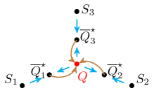
Figure 1: Illustration of the proposed algorithm. Consider three subgroups $S_{1},S_{2},S_{3}$, e.g., datasets for three different races. The proposed algorithm is then formulated as a bilevel optimization to learn an informative and fair predictive-distribution $Q$. In the lower-level (cyan), we learn the subgroup specific predictive-distribution $\overline{Q}^{\star}_{a}$ from dataset $S_{a}$ (limited samples) and the prior $Q$. In the upper-level (brown), $Q$ is then updated to be as close to all of the learned subgroup specific $\overline{Q}^{\star}_{a}$ as possible.

Controlling group sufficiency We adopted group sufficiency gap to measure fairness w.r.t. group sufficiency of a classifier $f$ (Sec.3), and then derive an upper bound of the group sufficiency gap (Theorem 4.1). Under proper assumptions, the upper bound is controlled by the discrepancy between the classifier $f$ and the subgroup Bayes predictors. Namely, minimizing the upper bound also encourages an informative classifier.

Algorithmic contribution Motivated by the upper bound of the group sufficiency gap, we develop a principled algorithm. Concretely, we adopt a randomized algorithm that produces a predictive-distribution $Q$ over the classifier ($f\sim Q$) to learn informative and fair classification. We further formulate the problem as a bilevel optimization (Sec. 5.3), as shown in Fig.1. (1) In the lower-level, the subgroup specific dataset $S_{a}$ and the fair predictive-distribution $Q$ are used to learn the subgroup specific predictive-distribution $\overline{Q}^{\star}_{a}$, where $Q$ is regarded as an informative prior for learning limited data within each subgroup. Theorem 5.1 formally demonstrates that under proper assumptions, the lower-level loss can effectively control the generalization error. (2) In the upper-level, the fair predictive-distribution $Q$ is then updated to be close to all subgroup specific predictive-distributions, in order to minimize the upper bound of the group sufficiency gap.

Empirical justifications  The proposed algorithm is applicable to the general parametric and differentiable model, where we adopt the neural network in the implementation. We evaluate the proposed algorithm on two real-world NLP datasets that have shown prediction disparities w.r.t. group sufficiency. Compared with baselines, the results indicate that group sufficiency has been consistently improved, with almost no loss of accuracy. Code is available at https://github.com/xugezheng/FAMS.

2 Related Work

Algorithmic fairness Fairness has been attached great importance and widely studied in various applications, such as natural language processing [8, 9, 10], natural language generation [11, 12, 13], computer vision [14, 15], and deep learning [16, 17]. Then various approaches have been proposed in algorithmic fairness. They typically add fair constraints during the training procedure, such as demographic parity or equalized odds [18, 19, 20, 21, 22, 23]. Apart from this, other fair notions are adopted such as accuracy parity [24, 25], which requires each subgroup to attain the same accuracy; small prediction variance [26, 27], which ensures small prediction variations among the subgroup; or small prediction loss for all the subgroups [28, 29, 30, 31]. Furthermore, based on the concept of Independence (e.g. demographic parity $A\perp\!\!\!\!\perp f(X)$) or conditional independence (e.g. equalized odds $A\perp\!\!\!\!\perp f(X)|Y$ or group sufficiency $A\perp\!\!\!\!\perp Y|f(X)$), another popular line in fair learning is then naturally integrated with information theoretical framework through adding mutual information constraints such as [32, 33].

Understanding fairness-accuracy trade-off As for the theoretical aspect, [34] further investigated the relation of fairness (demographic parity) and algorithmic stability. [35] formally justified the inherent trade-off between fairness (w.r.t. demographic parity and equalized odds) and accuracy, whereas the analysis is conducted for the binary sensitive attribute with the population loss. [36] studied the fair-accuracy trade-off in the multi-task learning.

Group sufficiency The fair notion of group sufficiency has recently been highlighted in various real-world scenarios such as health [6] and crime prediction [4, 37]. Specifically, [38] demonstrated that under proper assumptions, group sufficiency can be controlled in the unconstraint learning. However, this conclusion may not necessarily always hold in the overparameterized models with limited samples per subgroup, where [6, 39, 40] essentially revealed the prediction disparities between the different subgroups in the unconstraint learning. [41] recently studied the fair selective classification w.r.t. group sufficiency through an information theoretical framework, while the theoretical guarantee is unknown. In contrast, our proposed lower-level loss within the paper can provably control the generalization error, and the upper-level loss controls the group sufficiency gap. Besides, a close notion to the group sufficiency is the probability calibration [42], which is defined as $\mathbb{E}[Y|f(X)]=f(X)$ in binary classification. We will empirically show the probability calibration could be consistently improved within our framework, whereas the analysis on finite samples and its theoretical relation with group sufficiency remains still opening [43].

Bi-level optimization in fairness Bi-level optimization seeks to solve problems with a hierarchical structure. Namely, two levels of optimization problems where one task is nested inside another [44]. Several ideas related to bi-level optimization have been proposed in the context of fair-learning. For instance, we could design a min-max optimization to learn fair representation when considering demographic parity (DP) or equalized odds (EO) [19, 32, 25]. In this context, a representation function aims to minimize the loss caused by the discriminator in the lower-level. Simultaneously, in the upper-level, a discriminator could be introduced to maximize the loss. Then fair representation could be enforced through the bi-level optimization. Besides, if the accuracy and its variants are tracked as the metrics for each subgroup [12], the bi-level objective could also be deployed in controlling the loss [45] or the prediction variance [27], where the lower-level’s goal is to minimize the loss for each subgroup and the upper-level’s goal is to estimate the prediction disparities. In our paper, we theoretically justified a novel bi-level optimization perspective: controlling group sufficiency and accuracy. Simultaneously, other bi-level optimization and its relevant meta-learning algorithms could be further considered in the fair learning such as recurrent based gradient updating [46], layer-wise transformation [47] or implicit gradient based approach [48].

3 Preliminaries

We assume the joint random variable $(X,Y,A)$ follows an underlying distribution $\mathcal{D}(X,Y,A)$, where $X\in\mathcal{X}$ is the input, $Y\in\mathcal{Y}$ is the label, and the scalar discrete random variable $A\in\mathcal{A}$ denotes the sensitive attribute (or subgroup index). For instance, $A$ represents gender, race, or age. We also denote $\mathbb{E}[Y|X]$ as the conditional expectation of $Y$, which is essentially a function of $X$. $\mathbb{E}_{A,X}[\cdot]$ is denoted as the expectation on the marginal distribution of $\mathcal{D}(A,X)$. Throughout the paper, we consider binary classification with $\mathcal{Y}=\{0,1\}$. We further define the predictor as a scoring function $f:\mathcal{X}\to[0,1]$ that maps the input into a real value in $[0,1]$. It is worth mentioning that in general $f(X)\notin\mathcal{Y}$ since $f(X)$ is continuous. We then introduce group sufficiency and group sufficiency gap.

Definition 3.1 (Group sufficiency [1, 4, 38]).

A predictor $f$ satisfies group sufficiency with respect to the sensitive attribute $A$ if  $\mathbb{E}[Y|f(X)]=\mathbb{E}[Y|f(X),A]$.

Intuitively, given a output score of the predictor $f(X)=\tau$, the conditional expectation of $Y$ is invariant across different subgroups. Namely, conditioning on the specific subgroup $A=a$ does not provide any additional information about the conditional expectation of $Y$. Then we could naturally define group sufficiency gap.

Definition 3.2 (Group sufficiency gap [38]).

The group sufficiency gap of a predictor $f$ is defined as: $\textbf{Suf}_{f}=\mathbb{E}_{A,X}[\left|\mathbb{E}[Y|f(X)]-\mathbb{E}[Y|f(X),A]\right|]$

Specifically, $\textbf{Suf}_{f}$ measures the extent of group sufficiency violation, induced by the predictor $f$, which is taken by the expectation over $(X,A)$. Clearly, $\textbf{Suf}_{f}=0$ suggests that $f$ satisfies groups sufficiency and vice versa. For completeness, we also discuss other popular group fairness criteria: demographic parity and equalized odds.

Definition 3.3 (Demographic Parity (DP)).

A predictor $f$ satisfies the demographic parity with respect to the sensitive attribute $A$ if: $\mathbb{E}[f(X)]=\mathbb{E}[f(X)|A]$

Demographic Parity (DP), also known as statistical parity or independence rule, emphasizes that the expectation of the output score $f(X)$ is independent of $A$. [1, 4] further revealed that if $A\not\!\perp\!\!\!\perp Y$, group sufficiency and demographic parity could not be simultaneously achieved.

Definition 3.4 (Equalized Odds (EO) [18]).

A predictor $f$ satisfies the equalized odds with respect to $A$ if: $\mathbb{E}[f(X)|Y]=\mathbb{E}[f(X)|Y,A]$

Equalized odds (EO) emphasizes the conditional expectation of output $f$ is invariant w.r.t. $A$, given the ground truth $Y$. [1, 37] reveal that if $\mathcal{D}(X,Y,A)>0$ and $A\not\!\perp\!\!\!\perp Y$, group sufficiency and equalized odds can not both hold.

The analysis reveals a general incompatibility between group sufficiency and DP/EO when $A\not\!\perp\!\!\!\perp Y$, which often occurs in practice. Besides, DP/EO based criteria generally suffers the well-known fair accuracy trade-off [32]: enforcing the fair constraint degrades the prediction performance. This paper depicts that under the criteria of group sufficiency, these objectives could be both encouraged.

4 Upper bound of group sufficiency gap

To derive the theoretical results, we first introduce the group Bayes predictor.

Definition 4.1 ($A$-group Bayes predictor).

The $A$-group Bayes predictor $f_{A}^{\text{Bayes}}$ is defined as: $f_{A}^{\text{Bayes}}(X)=\mathbb{E}[Y|X,A]$

The $A$-group Bayes predictor is associated with the underlying data distribution $\mathcal{D}(X,Y,A)$. Given the fixed realization $X=x,A=a$, we have $f_{A=a}^{\text{Bayes}}(x)=\mathbb{E}[Y|X=x,A=a]$, which suggests the ground truth conditional data generation of subgroup $A=a$. By adopting $f_{A=a}^{\text{Bayes}}(x)$, we could derive the upper bound of group sufficiency gap w.r.t. any predictor $f$:

Theorem 4.1.

Group sufficiency gap $\textbf{Suf}_{f}$ is upper bounded by:  $\textbf{Suf}_{f}\leq 4\mathbb{E}_{A,X}[|f-f_{A}^{\text{Bayes}}|]$
Specifically, if $A$ takes finite value ($|\mathcal{A}|<+\infty$) and follows uniform distribution with $\mathcal{D}(A=a)=1/|\mathcal{A}|$. Then the group sufficiency gap is further simplified as:

$$\textbf{Suf}_{f}\leq\frac{4}{|\mathcal{A}|}\sum_{a}\mathbb{E}_{X}[|f-f_{A=a}^{\text{Bayes}}||A=a]$$

The proof is inspired by [38]. Specifically, Theorem 4.1 reveals that the upper bound of group sufficiency gap depends on the discrepancy between the predictor $f$ and $A$-group Bayes predictor $f_{A}^{\text{Bayes}}(X)$. Namely, given different subgroups $A=a$, the optimal predictor $f$ ought to be closed to all the group Bayes predictors $f_{A=a}^{\text{Bayes}}(X)$, $\forall a\in\mathcal{A}$.

Underlying assumption Theorem 4.1 also reveals underlying assumptions w.r.t. the data generation distribution $\mathcal{D}(X,Y,A)$ for achieving a small group sufficiency gap. If $f_{A}^{\text{Bayes}}$ for each subgroup $A=a$ are quite similar, then minimizing the upper bound yields a small group sufficiency gap $\textbf{Suf}_{f}$. For example, consider the extreme scenario if the $A$-group Bayes predictors are identical w.r.t. $A$, $\mathbb{E}[Y|X,A=a]=\mathbb{E}[Y|X],\forall a\in\mathcal{A}$, where $\mathbb{E}[Y|X]$ is the conventional Bayes predictor defined on the marginalized distribution $\mathcal{D}(X,Y)$. The upper bound recovers the difference between the predictor $f$ and standard Bayes predictor. If we use a probabilistic framework to approximate predictor $f(X)\approx\mathbb{E}[Y|X]$ (i.e, training the entire dataset without any fair constraint), both group sufficiency gap and prediction error (since Bayes predictor is optimal) will be small, which is consistent with [38]. On the contrary, if $A$-group Bayes predictors are completely arbitrary with high variance for $A$, both group sufficiency gap and prediction error are large and it would be impossible for an informative prediction.

5 Principled Approach

Based on the upper bound, we propose a principled approach to learn the predictor that achieves both small generalization error and group sufficiency gap.

5.1 Upper bound in randomized algorithm

To establish the theoretical result, we consider a randomized algorithm that learns a predictive-distribution $Q$ over scoring predictors from the data. For instance, if we consider Bayes framework, the predictor is drawn from the posterior distribution $\tilde{f}\sim Q$. In the inference, the predictor’s output is formulated as the expectation of the learned predictive-distribution $Q$: $f(X)=\mathbb{E}_{\tilde{f}\sim Q}\tilde{f}(X)$.

In practice, it is infeasible to optimize over all the possible distributions. Then we should restrict the predictive-distribution $Q$ within a distribution family $Q\in\mathcal{Q}$ such as Gaussian distribution. We also denote $Q_{a}^{\star}\in\mathcal{Q}$ as the optimal prediction-distribution w.r.t. $A=a$ under binary cross-entropy loss within the distribution family $\mathcal{Q}$:  $Q_{a}^{\star}:=\text{argmin}_{Q_{a}\in\mathcal{Q}}~{}\mathbb{E}_{\tilde{f}_{a}\sim Q_{a}}~{}\mathcal{L}_{a}^{\text{BCE}}(\tilde{f}_{a})$. In generally $Q^{\star}_{a}\neq f^{\text{Bayes}}(x,A=a)$, since the distribution family $\mathcal{Q}$ is only the subset of all possible distributions (shown in Fig. 2). We then extend the upper bound in the randomized algorithm.

Corollary 5.1.

The group sufficiency gap $\textbf{Suf}_{f}$ in randomized algorithm w.r.t. learned predictive-distribution $Q$ is upper bounded by:

$$\textbf{Suf}_{f}\leq\frac{2\sqrt{2}}{|\mathcal{A}|}[\sum_{a}\underbrace{\sqrt{\text{KL}(Q_{a}^{\star}\|Q)}}_{\text{Optimization}}+\underbrace{\sqrt{\text{KL}(Q_{a}^{\star}\|\mathcal{D}(Y|X,A=a))}}_{\text{Approximation}}]$$

Where KL is the Kullback–Leibler divergence. Corollary 5.1 further reveals that the upper bound is decomposed into two terms, showing in Fig.2.

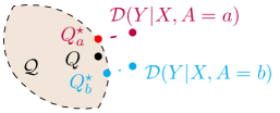
Figure 2: Illustration of optimization and approximation term. In the binary subgroup $\mathcal{A}=\{a,b\}$, the optimization term is to find $Q\in\mathcal{Q}$ to minimize the discrepancy between $(Q_{a}^{\star},Q_{b}^{\star})$. The approximation term is solely based on the distribution family $\mathcal{Q}$ (brown region). If the predefined $\mathcal{Q}$ has a rich expressive power, the approximation is treated as a small constant.

Optimization term  The optimization term is the average KL divergence between the learned distribution $Q$ and optimal predictive-distribution $Q^{\star}_{a}$ for each subgroup $A=a$. Minimizing the optimization term implies that the learned distribution $Q$ will be both fair and informative for the prediction, because it aims to minimize the upper bound of the group sufficiency gap $\textbf{Suf}_{f}$ and be close to the optimal predictive-distribution w.r.t. each $A=a$.

Approximation term  The approximation term is the average KL divergence between the optimal distribution $Q^{\star}_{a}$ and the underlying data generation distribution. Given the distribution family $\mathcal{Q}$, it is a unknown constant. Besides, if the distribution family $\mathcal{Q}$ has a rich expressive power such as deep neural-network, the approximation term will be small [49]. However, an extreme large distribution family $\mathcal{Q}$ could simultaneously yield a potential overfitting on finite samples. In this paper, the neural network is adopted and the approximation term is assumed to be a small constant. Thus, controlling $\textbf{Suf}_{f}$ implies minimizing the optimization term.

5.2 Challenge in learning limited samples

In practice, we only have access to finite or even limited samples in each subgroup, rather than the underlying distribution $\mathcal{D}$. We denote $S_{a}=\{(x^{a}_{i},y^{a}_{i})\}_{i=1}^{m}$ as the observed data w.r.t. subgroups $A=a$, which are i.i.d. samplings from the underlying distribution $\mathcal{D}(x,y|A=a)$. We also denote the empirical binary cross entropy loss w.r.t $A=a$ as: $\hat{\mathcal{L}}_{a}^{\text{BCE}}(\tilde{f})=\frac{1}{m}\sum_{i=1}^{m}-[y^{a}_{i}\log(\tilde{f}(x^{a}_{i}))+(1-y^{a}_{i})\log(1-\tilde{f}(x^{a}_{i}))]$. Then a straight approach is to minimize the empirical term $\hat{Q}_{a}^{\star}$:

$$\hat{Q}_{a}^{\star}=\text{argmin}_{Q_{a}\in\mathcal{Q}}~{}\mathbb{E}_{\tilde{f}_{a}\sim Q_{a}}~{}\hat{\mathcal{L}}_{a}^{\text{BCE}}(\tilde{f}_{a})$$ (1)

Then $Q$ is updated through minimizing the average KL-divergence: $\sum_{a}\text{KL}(\hat{Q}^{\star}_{a}\|Q)$ from learned $\hat{Q}_{a}^{\star}$. However, this idea generally does not work in our setting, because each subgroup contains limited number of samples. Therefore, a straight minimization leads to overfitting for each subgroup and generalization error $\mathbb{E}_{\tilde{f}\sim\hat{Q}^{\star}_{a}}~{}\mathcal{L}_{a}^{\text{BCE}}(\tilde{f})$ is quite large, showing in Fig. 5.

5.3 $Q$ as an informative prior

We have demonstrated that $Q$ can achieve both fair and informative prediction. Therefore, we regard $Q$ as a prior information for minimizing the loss, yielding a bilevel objective.

$$\min_{Q\in\mathcal{Q}}\frac{1}{|\mathcal{A}|}\sum_{a}\text{KL}(\overline{Q}_{a}^{\star}\|Q)$$ (Upper-level)

$$\text{s.t.}~{}~{}\overline{Q}_{a}^{\star}=\text{argmin}_{Q_{a}\in\mathcal{Q}}\{\mathbb{E}_{\tilde{f}_{a}\sim Q_{a}}~{}\hat{\mathcal{L}}_{a}^{\text{BCE}}(\tilde{f}_{a})+\lambda\text{KL}(Q_{a}\|Q)\},\forall a\in\mathcal{A}$$ (Lower-level)

Where $\lambda>0$ is the hyper-parameter. The proposed loss is a typical bilevel optimization. (1) In the lower-level, we aim to learn $\overline{Q}_{a}^{\star}$ for each $a\in\mathcal{A}$. Different from Eq. (1), the loss in lower-level adds a regularization term $\text{KL}(Q_{a}\|Q)$ as an informative prior in learning $\overline{Q}_{a}^{\star}$, given a fixed predictive-distribution $Q$. Moreover, Theorem 5.1 formally justified that optimizing the lower-level loss is to minimize the upper bound of the generalization error. (2) In the upper-level, $Q$ is updated through minimizing the average KL divergence between different $\overline{Q}_{a}^{\star}$, which controls the upper bound of $\textbf{Suf}_{f}$.

Theorem 5.1 (Generalization error bound).

Supposing that datasets $\{S_{a}\}_{a=1}^{|\mathcal{A}|}$ with $S_{a}=\{(x^{a}_{i},y^{a}_{i})\}_{i=1}^{m}$ are i.i.d. sampled from $\mathcal{D}(x,y|A=a)$, the binary cross entropy (BCE) loss is upper bounded by $L$, $Q_{a}\in\mathcal{Q}$ is any learned distribution from dataset $S_{a}$ and $Q\in\mathcal{Q}$ is any distribution. Then with high probability $\geq 1-\delta$ with $\forall\delta\in(0,1)$, we have:

$$\small\frac{1}{|\mathcal{A}|}\sum_{a}\mathbb{E}_{\tilde{f}_{a}\sim Q_{a}}\mathcal{L}_{a}^{\text{BCE}}(\tilde{f}_{a})\leq\underbrace{\frac{1}{|\mathcal{A}|}\sum_{a}\mathbb{E}_{\tilde{f}_{a}\sim Q_{a}}\hat{\mathcal{L}}_{a}^{\text{BCE}}(\tilde{f}_{a})}_{(1)}+\underbrace{\frac{L}{\sqrt{|\mathcal{A}|m}}\sum_{a}\sqrt{\text{KL}(Q_{a}\|Q)}}_{(2)}+\underbrace{L\sqrt{\frac{\log(1/\delta)}{|\mathcal{A}|m}}}_{(3)}$$

Discussions  The proof is inspired by PAC-Bayes theorem such as [50, 51, 52]. Secpficially, Theorem 5.1 reveals the generalization error in the lower-level is upper bounded by three terms. (a) Term (1) is the average empirical prediction error, which corresponds to the first term in the lower-level loss. (b) Term (2) indicates the average KL-divergence between the learned subgroup distribution $Q_{a}$ and the prior distribution $Q$, which corresponds to the second term in the lower-level loss. The combination of term (1-2) recovers the averaged lower-level loss w.r.t. $A$. Thus optimizing the lower-level loss could control the generalization error. (c) When the confidence $\delta$ is fixed, term (3) will converge if $|\mathcal{A}|m\to+\infty$. Moreover, even if $m$ (the sample size in each subgroup) is quite small, a sufficient large number of subgroups $|\mathcal{A}|$ can also ensure the convergence of term (3).

For the sake of simplicity, we assumed the identical samples size $m$ in each subgroup $S_{a}$, while the theoretical result can be extended to subgroups with different samples $m_{a}$.

5.4 Practical Implementations

In this section, we develop a practical learning algorithm that can be applied to a wide range of differentiable and parametric models, including neural networks.

Parametric models

We choose the Isotropic Gaussian distribution (with diagonal covariance matrix) as the distribution family $\mathcal{Q}$, where the mean and covariance are set as $d$-dimensional parameter. Thus we need to learn the parameter $(\bm{\theta},\bm{\sigma})$ for fair and informative $Q\in\mathcal{Q}$. As for the subgroup $A=a$, we learn parameters $(\bm{\theta}_{a},\bm{\sigma}_{a})$ for $\overline{Q}^{\star}_{a}\in\mathcal{Q}$. It is worth mentioning that the Isotropic Gaussian distribution is selected for its computational efficiency in the optimization. We can use any distribution as long as the density function is differentiable with respect to the parameters.

For the single predictor $\tilde{f}$, we use parametric neural-network models and assume $\tilde{f}$ is parameterized by a $d$-dimensional vector ${\bf{w}}\in\mathbb{R}^{d}$, denoted as $\tilde{f}_{\bf{w}}$. Then $\tilde{f}_{\bf{w}}\sim Q$ is equivalent to sampling the model parameter $\bf{w}$ from the predictive-distribution $Q$: $\mathbf{w}\sim\mathcal{N}(\bm{\theta},\bm{\sigma}^{2})=\prod_{i=1}^{d}\mathcal{N}(\bm{\theta}[i],\bm{\sigma}^{2}[i])$. Since $Q$ is Isotropic Gaussian, each element $i$ in the parameter ${\bf w}[i]$ follows a 1-dimensional Gaussian. Following the same line, $\tilde{f}_{{\bf{w}}_{a}}\sim\overline{Q}^{\star}_{a}$ can be modeled analogously: $\mathbf{w}_{a}\sim\mathcal{N}(\bm{\theta}_{a},\bm{\sigma}_{a}^{2})=\prod_{i=1}^{d}\mathcal{N}(\bm{\theta}_{a}[i],\bm{\sigma}^{2}_{a}[i])$. As a result, learning the distribution $Q$ is equivalent to learning parameter $(\bm{\theta},\bm{\sigma})$ in the bilevel objective.

Gradient Estimation

Based on the previous setting, we aim to optimize the bilevel objective to obtain the parameter of $Q$: $(\bm{\theta},\bm{\sigma})$. We use stochastic gradient descent (SGD) to optimize the parameters. In the lower-level, the loss in Sec. 5.3 is composed by the empirical prediction error and KL divergence term. The KL divergence has a closed form that can be differentiated efficiently. Specifically, since $Q$ and the subgroup specific $\overline{Q}^{\star}_{a}$ are factorized Gaussian, the KL divergence takes a simple closed form and the gradient can be easily calculated: $\text{KL}(\overline{Q}^{\star}_{a}\|Q)=\frac{1}{2}\sum_{i=1}^{d}\left\{\log\frac{\bm{\sigma}^{2}_{a}[i]}{\bm{\sigma}^{2}[i]}+\frac{\bm{\sigma}^{2}_{a}[i]+(\bm{\theta}_{a}[i]-\bm{\theta}[i])^{2}}{\bm{\sigma}^{2}[i]}-1\right\}$.

Re-parametrization trick

As for the prediction error $\mathbb{E}_{\tilde{f}_{{\bf{w}}_{a}}\sim Q_{a}}~{}\hat{\mathcal{L}}_{a}^{\text{BCE}}(\tilde{f}_{{\bf{w}}_{a}})$, the term $\hat{\mathcal{L}}_{a}^{\text{BCE}}(\tilde{f}_{{\bf{w}}_{a}})$ is non-linear for $\bf{w}$, rendering the expectation intractable in the computation. To this end, we adopt the re-parameterization trick [53, 54] in computing the gradient w.r.t. the expectation term. The trick is based on describing the Gaussian distribution ${\bf{w}}_{a}\sim\mathcal{N}({\bm{\theta}}_{a},{\bm{\sigma}}^{2}_{a})$ as first drawing $\bm{\epsilon}\sim\mathcal{N}(\mathbf{0},\mathbf{I})$ and then applying the deterministic function ${\bf{w}}_{a}({\bm{\theta}}_{a},{\bm{\sigma}}_{a})=\bm{\theta}_{a}+\bm{\sigma}_{a}\odot\bm{\epsilon}$ ($\odot$ is element-wise product) to approximate the sampling. Then the gradient term can be estimated as: $\nabla_{({\bm{\theta}}_{a},{\bm{\sigma}}_{a})}\mathbb{E}_{{\bf{w}}_{a}\sim N({\bm{\theta}}_{a},{\bm{\sigma}}_{a})}~{}\hat{\mathcal{L}}_{a}^{\text{BCE}}(\tilde{f}_{{\bf{w}}_{a}})=\nabla_{(\bm{\theta}_{a},\bm{\sigma}_{a})}\mathbb{E}_{\bm{\epsilon}\sim\mathcal{N}(\mathbf{0},\mathbf{I})}\hat{\mathcal{L}}_{a}^{\text{BCE}}(\tilde{f}_{{\bf{w}}_{a}({\bm{\theta}}_{a},{\bm{\sigma}}_{a})})$, where the expectation can be approximated by Monte-Carlo sampling w.r.t. $\bm{\epsilon}$. For a fixed sample $\bm{\epsilon}$, the gradient can be computed through backpropagation. In the upper-level, the KL divergence has a closed form, thus it is easy to update the parameter of $Q$ through backpropagation.

Proposed Algorithm

Based on the analysis, the algorithm is shown in Algorithm. 1 for solving the bilevel objective in Sec. 5.3. Specifically, we adopt the alternating optimization. Namely, in the lower-level, we fix $Q$ and optimize the subgroup specific predictor $\overline{Q}^{\star}_{a}$ through SGD. Then in the upper-level, we fix the learned $\overline{Q}^{\star}_{a}$ and update $Q$. Since we may face many subgroups, at each training epoch, we randomly sample a subset $\mathcal{A}^{{}^{\prime}}$ such that $|\mathcal{A}^{{}^{\prime}}|\ll|\mathcal{A}|$ for the memory saving.

Algorithm 1 Fair and Informative Learning for Multiple Subgroups (FAMS)

1:  Input: Parameters w.r.t. distribution $Q$:$(\bm{\theta},\bm{\sigma}^{2})$, datasets $\{S_{a}\}$, $a\in\mathcal{A}$.

2:  for Sampling a subset of $\{S_{a}\}$, where $a\in\mathcal{A}^{\prime}\subseteq\mathcal{A}$ do

3:     ### Solving the lower-level ###

4:     Fix $Q$, optimizing the loss w.r.t. $Q_{a}=\mathcal{N}(\bm{\theta}_{a},\bm{\sigma}^{2}_{a})$ through SGD for each $a\in\mathcal{A}^{\prime}$ $\quad\quad\quad\quad\quad\quad\quad\quad\quad\mathbb{E}_{\tilde{f}_{{\bf w}_{a}}\sim Q_{a}}~{}\hat{\mathcal{L}}_{a}^{\text{BCE}}(\tilde{f}_{{\bf w}_{a}})+\lambda\text{KL}(Q_{a}\|Q)$

5:     Obtaining the solution $\overline{Q}^{\star}_{a}$, $a\in\mathcal{A}^{\prime}$.

6:     ### Solving the upper-level ###

7:     Fix $\overline{Q}^{\star}_{a}$ with $a\in\mathcal{A}^{\prime}$, optimizing the loss w.r.t. $Q$ through SGD: $\frac{1}{|\mathcal{A}^{\prime}|}\sum_{a}\text{KL}(\overline{Q}_{a}^{\star}\|Q)$

8:     Obtaining updated parameter $(\bm{\theta},\bm{\sigma}^{2})$ in $Q$

9:  end for

10:  Return:  Parameter of distribution $Q$: $(\bm{\theta},\bm{\sigma}^{2})$

Inference

In the inference, we use the Monte-Carlo method to sample the weights of the neural network from distribution ${\bf{w}}\sim\mathcal{N}(\bm{\theta},\bm{\sigma}^{2})$, then averaging the output w.r.t. different sampled weights to approximate $f(x)=\mathbb{E}_{\tilde{f}_{\bf{w}}\sim Q}\tilde{f}_{\bf{w}}(x)$

6 Experiments

6.1 Experimental Setup

Dataset: Amazon review

We adopt Amazon review dataset [55, 40], which aims to predict the sentiment (classification) from the review. The datasets consist of large-scale users. Each user has limited number of reviews, ranging from 75 to 400. The user is then treated as a subgroup, and it has been observed that standard training can lead to prediction disparities in several users.[56].The experiment is adapted from the protocol of [40]. Specifically, we convert the original review score (ranging from 1-5) to the binary label: the positive review (score $\geq 4$) and negative review (score $\leq 3$). We draw and then fix 200 users from the original dataset, which includes the training, validation, and test sets. In the implementation, we first adopt DistilBERT [57] to learn the embedding with dimension $\mathbb{R}^{768}$. Then we adopt $\tilde{f}_{\bf{w}}$ and $\tilde{f}_{\bf{w}_{a}}$ as the four-layer fully connected neural network, where ${\bf w}\sim Q$ and ${\bf w}_{a}\sim Q_{a}$. Additional experimental details are delegated to the Appendix.

Dataset: Toxic Comments

We also use the toxic comment dataset [58] to predict the text comment being toxic or not, which has shown the significant performance degradation on specific sub-populations. Following [58], we select race as sensitive attribute, which includes Black, White, Asian and Latino & others (4 subgroups). We also follow the same setting as the original dataset [40], which has the separate training, validation, and test sets. Since toxic comments are marked by multiple annotators, we decide that the comment is toxic if it is marked by at least half of the annotators. In the implementation, we adopt the DistilBERT [57] as the embedding with output dimension $\mathbb{R}^{768}$. Then we also adopt $\tilde{f}_{\bf{w}}$ and $\tilde{f}_{\bf{w}_{a}}$ as the four-layer fully connected neural network, with the same network structure as Amazon. Additional details are delegated to the Appendix.

Baselines

We compare with following baselines. (1) ERM: training a deep model without considering the sensitive attribute. (2) SNN. Since we adopt randomized algorithms in the paper, we additionally compare the stochastic neural network through the vanilla training from the whole dataset. Namely, we find a predictive-distribution $Q$ to minimize $\frac{1}{|\mathcal{A}|}\sum_{a}\mathbb{E}_{f\sim Q}\hat{\mathcal{L}}_{a}^{\text{BCE}}(f)$. (3) EIIL [43] proposed an IRM based approach to promote the group sufficiency. (4) FSCS [41] adopted the conditional mutual information constraint $I(A,Y|f(X))$ to promote the sufficiency. (5) DRO [24]. A re-weighting approach to assign the importance of the task. Indeed, DRO does not provably guarantee group sufficiency, while it encourages identical losses. All the experiments are repeated five times.

Computing $\textbf{Suf}_{f}$

Since $f(X)$ is continuous, the group sufficiency gap is calculated by splitting the output of predictor into multiple intervals in $[0,1]$ and computing the conditional expectation within each interval, as detailed in Appendix.

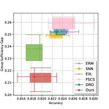
(a) Accuracy-$\textbf{Suf}_{f}$

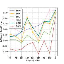
(b) $\textbf{Suf}_{f}$ on each subgroup

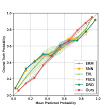
(c) Probability Calibration

Figure 3: Amazon Review dataset. (a) Boxplot of accuracy and group sufficiency gap $\textbf{Suf}_{f}$ with 5 repeats: median, 75th percentile and minimum-maximum value. (b) Group sufficiency gap on subgroup $A=a$, which is the difference between $\mathbb{E}[Y|f(X)]$ and $\mathbb{E}[Y|f(X),A=a]$. We visualize the top-9 users’ group sufficiency gap in ERM, whereas the result for all users is delegated to the Appendix. (c) Probability calibration curve over 5 repeats with mean and standard deviation. i.e $(f(X),\mathbb{E}[Y|f(X)])$. The proposed approach demonstrated a consistently improved probability calibration.

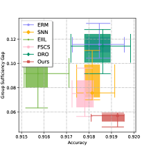
(a) Accuracy-$\textbf{Suf}_{f}$

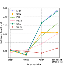
(b) $\textbf{Suf}_{f}$ on each subgroup

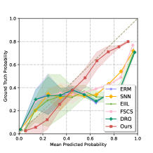
(c) Probability Calibration

Figure 4: Toxic dataset. (a) Boxplot of accuracy and group sufficiency gap $\textbf{Suf}_{f}$ with 5 repeats: median, 75th percentile and minimum-maximum value. (b) Group sufficiency gap on the specific subgroup $A=a$, which is the difference between $\mathbb{E}[Y|f(X)]$ and $\mathbb{E}[Y|f(X),A=a]$. (c) Probability calibration over 5 repeats with mean and standard deviation. i.e $(f(X),\mathbb{E}[Y|f(X)])$, where the probability calibration for each subgroup is delegated to Appendix.

6.2 Experimental Results

We visualize the results in Fig. 3 for Amazon review product and Fig. 4 for toxic comment.

Accuracy and Fairness The accuracy and group sufficiency gap are depicted in Fig. 3(a) and Fig. 4(a). In Amazon review, the accuracy in the proposed approach has a slight decrease, compared with ERM. While the group sufficiency gap has improved by $3.0\%$, showing a significant improvement in the fairness. In toxic comments, the accuracy in proposed approach is nearly identical to the baseline, whereas group sufficiency gap has been significantly improved by $3.0$-$3.5\%$.

Group sufficiency gap on the specific subgroup To gain better understandings of group sufficiency gap, we visualize group sufficiency gap on specific subgroup $A=a$, i.e the discrepancy between the $\mathbb{E}[Y|f(X)]$ (conditional expectation on the entire data) and $\mathbb{E}[Y|f(X),A=a]$ (conditional expectation on subgroup $A=a$). I.e, $\mathbb{E}_{X}\left[|\mathbb{E}[Y|f(X)]-\mathbb{E}[Y|f(X),A=a]|\right]$.

In Amazon review dataset, we visualize the top-9 users’ sufficiency gap in ERM, as shown in Fig. 3(b), where the gap of entire users is delegated to the Appendix. The proposed approach significantly reduces the group sufficiency gap of in most subgroups. The similar trend is also observed in Toxic dataset, as shown in Fig. 4(b), where the proposed approach has the nearly identical and small group sufficiency gap for each race. In contrast, the baselines exhibit significant group sufficiency bias on the Asian and Latino & other races.

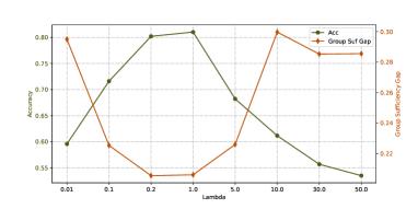
Figure 5: Analysis. Accuracy-$\textbf{Suf}_{f}$ curve under different $\lambda$ in Amazon review dataset.

Probability Calibration A related concept to group sufficiency is the probability calibration [42], which is defined as $\mathbb{E}[Y|f(X)]=f(X)$ in the binary classification. We visualize the probability sufficiency of Amazon review in Fig. 3(c) and Toxic comments in Fig. 4(c). The results suggest that the proposed approach demonstrates a consistently better probability calibration on the whole data. We then visualize the probability calibration for each subgroup, as shown in the Appendix, where the results reveal the improved probability calibration for each subgroup.

Other sensitive attributes in Toxic comments Apart from adopting race as sensitive attribute, we also consider other possible sensitive attributes such as gender and religion, and the results are showed in the Appendix. The results in other sensitive attributes are similar to race, with improved fairness and no loss on accuracy.

Influence of $\lambda$. Fairness and accuracy can be simultaneously achieved. Theorem 5.1 suggests that there exists an optimal $\lambda$ in the generalization error bound. Then we changed the value of $\lambda$ in Amazon dataset, as shown in Fig. 5.

When $\lambda\to 0$, the subgroup specific parameters are simply learned from the limited samples within each subgroup. Then the fair predictor could not learn a proper prior from the subgroup specific predictor with a significant generalization error. Meanwhile, the group sufficiency gap is also large, which is consistent with [38]: overfitting generally degrades the group sufficiency. When $\lambda$ is set between $[0.2,1]$, the generalization error is small (with a high accuracy) and group sufficiency gap is kept small, implying that both fairness and accuracy can be achieved. In contrast, if we set a large value for $\lambda\gg 0$, the predictor is unable to learn from the data but from the random prior $Q$. The prediction will be completely random (accuracy $=55\%$ when $\lambda=50$). When the predictor outputs a random guess, different from demographic parity (DP) or equalized odds (EO), the group sufficiency gap is also large. The analysis reveals that there exists an optimal $\lambda$ for simultaneously achieving accuracy and group sufficiency.

7 Conclusion

We conducted a novel analysis by simultaneously learning an informative and fair classifier for multiple or even many subgroups. We derived a novel principled algorithm. We further theoretically justified the generalization error and fair guarantees of the proposed framework. The empirical results in two real-world datasets demonstrated the effectiveness in both preserving the accuracy, as well as group sufficiency.

Discussion on Limitations

We proposed the analysis on learning group sufficiency and informative predictors, and developed a principled approach for it. Simultaneously there are several limitations to the proposed theory and algorithm. (1) In general, group sufficiency and DP/EO are incompatible. Controlling group sufficiency, for example, would cause DP/EO degradation. This would be problematic if DP/EO were preferred in practice. (2) We also assumed that the ground truth $A$-Bayes predictors would be similar across groups. However, this assumption could be violated, resulting in a highly non-trivial scenario. Thus, in order to evaluate the conditional distribution shift, we need to consider a new setting by collect sufficient data per subgroup.

Checklist

The checklist follows the references. Please read the checklist guidelines carefully for information on how to answer these questions. For each question, change the default [TODO] to [Yes] , [No] , or [N/A] . You are strongly encouraged to include a justification to your answer, either by referencing the appropriate section of your paper or providing a brief inline description. For example:

• Did you include the license to the code and datasets? [Yes] See Section LABEL:gen_inst.

• Did you include the license to the code and datasets? [No] The code and the data are proprietary.

• Did you include the license to the code and datasets? [N/A]

Please do not modify the questions and only use the provided macros for your answers. Note that the Checklist section does not count towards the page limit. In your paper, please delete this instructions block and only keep the Checklist section heading above along with the questions/answers below.

1. For all authors…

   1. Do the main claims made in the abstract and introduction accurately reflect the paper’s contributions and scope? [Yes]

   2. Did you describe the limitations of your work? [Yes] The proposed theoretical analysis is restricted in the randomized algorithm.

   3. Did you discuss any potential negative societal impacts of your work? [Yes] We study the algorithmic fairness. It is worth noting that ensuring group sufficiency may degrade other fair criteria such as DP/EO.

   4. Have you read the ethics review guidelines and ensured that your paper conforms to them? [Yes]

2. If you are including theoretical results…

   1. Did you state the full set of assumptions of all theoretical results? [Yes] In the paper and Appendix.

   2. Did you include complete proofs of all theoretical results? [Yes] In Appendix.

3. If you ran experiments…

   1. Did you include the code, data, and instructions needed to reproduce the main experimental results (either in the supplemental material or as a URL)? [Yes] We provided the code for the reproduction.

   2. Did you specify all the training details (e.g., data splits, hyperparameters, how they were chosen)? [Yes] See the source code.

   3. Did you report error bars (e.g., with respect to the random seed after running experiments multiple times)? [Yes] We visualize the Boxplot of the results.

   4. Did you include the total amount of compute and the type of resources used (e.g., type of GPUs, internal cluster, or cloud provider)? [N/A]

4. If you are using existing assets (e.g., code, data, models) or curating/releasing new assets…

   1. If your work uses existing assets, did you cite the creators? [N/A]

   2. Did you mention the license of the assets? [N/A]

   3. Did you include any new assets either in the supplemental material or as a URL? [N/A]

   4. Did you discuss whether and how consent was obtained from people whose data you’re using/curating? [N/A]

   5. Did you discuss whether the data you are using/curating contains personally identifiable information or offensive content? [N/A]

5. If you used crowdsourcing or conducted research with human subjects…

   1. Did you include the full text of instructions given to participants and screenshots, if applicable? [N/A]

   2. Did you describe any potential participant risks, with links to Institutional Review Board (IRB) approvals, if applicable? [N/A]

   3. Did you include the estimated hourly wage paid to participants and the total amount spent on participant compensation? [N/A]

Appendix A Group sufficiency vs. demographic parity (DP) and equalized odds (EO)

For better understanding the properties of these three metrics, we consider the following scenario.

Consider the score predictor $f(X)$ uniformly outputs a value in $[0,1]$ for any $x\in\mathcal{X}$. i.e, $f(x)\sim\text{Unif}[0,1]$. Then it is easy to verify the demographic party and equalized odds both satisfy. Since the output of predictor is completely independent with the data. Thus we have

$$\mathbb{E}[f(X)]=\mathbb{E}[f(X)|A],\mathbb{E}[f(X)|Y]=\mathbb{E}[f(X)|A,Y]$$

In contrast, the group sufficiency does not necessarily hold. Specifically we have $\mathbb{E}[Y|f(X)]=\mathbb{E}[Y],\mathbb{E}[Y|f(X),A]=\mathbb{E}[Y|A]$, then we have

$$\textbf{Suf}_{f}=\mathbb{E}_{A}|\mathbb{E}[Y]-\mathbb{E}[Y|A]|>0,$$

if $A\not\!\perp\!\!\!\perp Y$.

The aforementioned counterexample suggests that group sufficiency shows different behaviors, where the pure random prediction could trivially achieve the EO/DP.

Moreover, based on [1], if $\mathcal{D}(X,Y,A)>0$ and $A\not\!\perp\!\!\!\perp Y$, the group sufficiency and demographic parity/equalized odds do not both hold. The aforementioned example also verifies this fact.

Appendix B Additional Facts of $A$-Group Bayes predictor

For better understanding $A$-Group Bayes predictor, we could derive the following facts.

Proposition B.1.

The $A$-group Bayes predictor $f_{A}^{\text{Bayes}}(X)$: (1) Given a subgroup $A=a$, satisfies the group sufficiency $\mathbb{E}[Y|f_{A=a}^{\text{Bayes}}(X)]=\mathbb{E}[Y|f_{A=a}^{\text{Bayes}}(X),A=a]$; (2) is the optimal predictor under subgroup $A=a$ the binary cross-entropy loss function. Namely, $f_{A=a}^{\text{Bayes}}(x)=\text{argmin}_{f}\mathcal{L}^{\text{BCE}}_{a}(f)$, where $\mathcal{L}^{\text{BCE}}_{a}(f)=\mathbb{E}_{(x,y)\sim\mathcal{D}(x,y|A=a)}-[y\log(f(x))+(1-y)\log(1-f(x))]$.

Proposition B.1 shows that given a subgroup $A=a$, $A$-group Bayes predictor simultaneously meets both fairness (group sufficiency) and informative (optimal predictor under binary cross-entropy loss). Unfortunately, $f^{\text{Bayes}}$ is impossible to estimate since it is related to the underlying data distribution $\mathcal{D}$, which is infeasible. Nevertheless, we can adopt $A$-group Bayes predictor $f^{\text{Bayes}}$ to derive an upper bound of group sufficiency gap $\textbf{Suf}_{f}$. The upper bound then holds for any predictor $f$ that can be learned from the observed data.

B.1 Proof of Fact 1

We first introduce the generalized Tower rule of the conditional expectation.

Generalized tower rule of conditional expectation

Let $(\Omega,\mathcal{F},P)$ be the probability space and two sub $\sigma$-algebras $\mathcal{G}_{1}\subseteq\mathcal{G}_{2}\subseteq\mathcal{F}$ are defined. Then we have

$$\mathbb{E}[\mathbb{E}[X|\mathcal{G}_{2}]|\mathcal{G}_{1}]=\mathbb{E}[X|\mathcal{G}_{1}]$$

Proof.

Based on the generalized tower rule, we have

$$\mathbb{E}[Y|f_{A}^{\text{Bayes}}(X),A] =\mathbb{E}[\mathbb{E}[Y|X,A,f_{A}^{\text{Bayes}}(X)]|f_{A}^{\text{Bayes}}(X),A]$$

$$=\mathbb{E}[\mathbb{E}[Y|X,A]|f_{A}^{\text{Bayes}}(X),A]=\mathbb{E}[f_{A}^{\text{Bayes}}|f_{A}^{\text{Bayes}}(X),A]=f_{A}^{\text{Bayes}}(X)$$

Also we have:

$$\mathbb{E}[Y|f_{A}^{\text{Bayes}}(X)] =\mathbb{E}[\mathbb{E}[Y|f_{A}^{\text{Bayes}}(X),A,X]|f_{A}^{\text{Bayes}}(X)]$$

$$=\mathbb{E}[\mathbb{E}[Y|f_{A}^{\text{Bayes}}(X),A,X]|f_{A}^{\text{Bayes}}(X)]$$

$$=\mathbb{E}[\mathbb{E}[Y|A,X]|f_{A}^{\text{Bayes}}(X)]=\mathbb{E}[f_{A}^{\text{Bayes}}(X)|f_{A}^{\text{Bayes}}(X)]=f_{A}^{\text{Bayes}}(X)$$

Combining these two equations, we have the Fact 1:

$$\mathbb{E}[Y|f_{A}^{\text{Bayes}}(X),A]=\mathbb{E}[Y|f_{A}^{\text{Bayes}}(X)]$$

The aforementioned proof adopts the fact $\mathbb{E}[Y|f_{A}^{\text{Bayes}}(X),A,X]=\mathbb{E}[Y|A,X]$, since the conditional expectation is uninfluenced by the $A$-group Bayes predictor, given $A,X$. ∎

B.2 Proof of Fact 2

Following [59], we can compute the optimal predictor of attribute $A=a$ under the binary cross-entropy by taking the functional derivative w.r.t. $f$:

$$\frac{d\mathcal{L}_{a}^{\text{BCE}}(f)}{df}=0$$

We have

$$\mathbb{E}_{\mathcal{D}(x,y|a)}[f(x)-y]=0$$

$$\to \mathbb{E}_{\mathcal{D}(x|a)}[f(x)\mathbb{E}_{\mathcal{D}(y|x,a)}-\mathbb{E}_{\mathcal{D}(y|x,a)}y]=0$$

$$\to \mathbb{E}_{\mathcal{D}(x|a)}[f(x)-\mathbb{E}_{\mathcal{D}(y|x,a)}y]=0$$

Therefore, we have the optimal predictor $f^{\star}=\mathbb{E}_{\mathcal{D}(y|x,a)}y=\mathbb{E}[Y=y|X=a,A=a]$, the $A$-group Bayes predictor. [59] further demonstrated the optimal is unique under the binary cross entropy loss.

Appendix C Upper bound of group sufficiency gap

Before deriving the theory, we need the following lemma.

Lemma C.1.

For any predictor $f$, we have

$$\mathbb{E}[Y|f(X),A]=\mathbb{E}[f_{A}^{\text{Bayes}}(X)|f(X),A]$$

Proof.

$$\mathbb{E}[Y|f(X),A] =\mathbb{E}[\mathbb{E}[Y|f(X),A,X]|f(X),A]$$

$$=\mathbb{E}[\mathbb{E}[Y|A,X]|f(X),A]$$

$$=\mathbb{E}[f_{A}^{\text{Bayes}}(X)|f(X),A]$$

∎

Based on Lemma B.1, we can derive the main Theorem.

Proof.

For the simplicity, we denote $\mathbb{E}[Y|f,A]=\mathbb{E}[Y|f(X),A]$ and $\mathbb{E}[Y|f_{A}^{\text{Bayes}},A]=\mathbb{E}[Y|f_{A}^{\text{Bayes}}(X),A]$. We first bound $\mathbb{E}_{A,X}[|\mathbb{E}[Y|f,A]-\mathbb{E}[Y|f_{A}^{\text{Bayes}},A]|]$

$$\mathbb{E}_{A,X}[|\mathbb{E}[Y|f,A]-\mathbb{E}[Y|f_{A}^{\text{Bayes}},A]|] =\mathbb{E}_{A,X}[|\mathbb{E}[f_{A}^{\text{Bayes}}|f,A]-f_{A}^{\text{Bayes}}|]$$

$$=\mathbb{E}_{A,X}[|\mathbb{E}[f_{A}^{\text{Bayes}}-f|f,A]+f-f_{A}^{\text{Bayes}}|]$$

$$\leq\mathbb{E}_{A,X}[|\mathbb{E}[f_{A}^{\text{Bayes}}-f|f,A]|+|f-f_{A}^{\text{Bayes}}|]$$

$$=2\mathbb{E}_{A,X}[|f-f_{A}^{\text{Bayes}}|]$$

Where $\mathbb{E}_{A,X}[|\mathbb{E}[f_{A}^{\text{Bayes}}-f|f,A]|]=\mathbb{E}_{A,X}[\mathbb{E}|f_{A}^{\text{Bayes}}-f|f,A,X|]=\mathbb{E}_{A,X}[|\mathbb{E}[f_{A}^{\text{Bayes}}-f|A,X]|]=\mathbb{E}_{A,X}[|f_{A}^{\text{Bayes}}-f|]$ is derived from the tower rule of conditional expectation.

Analogously, we can bound

$$\mathbb{E}_{A,X}[|\mathbb{E}[Y|f]-\mathbb{E}[Y|f_{A}^{\text{Bayes}}]|]\leq 2\mathbb{E}_{A,X}[|f-f_{A}^{\text{Bayes}}|]$$

Thus the group sufficiency gap is upper bounded by:

$$\textbf{Suf}_{f} =\mathbb{E}_{A,X}[|\mathbb{E}[Y|f]-\mathbb{E}[Y|f,A]|]$$

$$=\mathbb{E}_{A,X}[|\mathbb{E}[Y|f]-\mathbb{E}[Y|f,A]-\mathbb{E}[Y|f_{A}^{\text{Bayes}}]-\mathbb{E}[Y|f_{A}^{\text{Bayes}},A]|]~{}~{}(\text{Using Fact 1})$$

$$\leq\mathbb{E}_{A,X}[|\mathbb{E}[Y|f]-\mathbb{E}[Y|f_{A}^{\text{Bayes}}]|+|\mathbb{E}[Y|f,A]-\mathbb{E}[Y|f_{A}^{\text{Bayes}},A]|]$$

$$\leq 4\mathbb{E}_{A,X}[|f-f_{A}^{\text{Bayes}}|]$$

Therefore, if $A$ takes only finite value ($|\mathcal{A}|<+\infty$) and follows uniform distribution with $\mathcal{D}(A=a)=1/|\mathcal{A}|$, then we have:

$$\textbf{Suf}_{f}\leq\frac{4}{|\mathcal{A}|}\sum_{a}\mathbb{E}_{X}[|f-f_{A=a}^{\text{Bayes}}||A=a]$$

∎

Appendix D Upper bound of group sufficiency gap in randomized algorithm

According to the definition, we have:

$$\textbf{Suf}_{f} \leq\frac{4}{|\mathcal{A}|}\sum_{a}\mathbb{E}_{X}[|\mathbb{E}_{\tilde{f}\sim Q}\tilde{f}(x)-\mathbb{E}_{\tilde{f}\sim Q_{a}^{\star}}\tilde{f}(x)|+|\mathbb{E}_{\tilde{f}\sim Q_{a}^{\star}}\tilde{f}(x)-\mathbb{E}_{\tilde{f}\sim\mathcal{D}(y|x,a)}\tilde{f}(x)|]$$

$$\leq\frac{4}{|A|}\sum_{a}\text{TV}(Q_{a}^{\star}\|Q)+\text{TV}(Q_{a}^{\star}\|\mathcal{D}(y|x,a))~{}~{}~{}(\text{Property of Total variation distance})$$

$$\leq\frac{2\sqrt{2}}{|A|}[\sum_{a}\underbrace{\sqrt{\text{KL}(Q_{a}^{\star}\|Q)}}_{\text{Estimation Error}}+\underbrace{\sqrt{\text{KL}(Q_{a}^{\star}\|\mathcal{D}(y|x,a))}}_{\text{Approximation Error}}]~{}~{}~{}(\text{Pinsker's inequality})$$

The second line is derived from the property of Total variation distance. Note the scoring predictor ranges in $[0,1]$: $\tilde{f}(X=x)\in[0,1]$.

The third line is derived from Pinsker’s inequality. i.e, $\text{TV}(P\|Q)\leq\sqrt{\frac{1}{2}\text{KL}(P\|Q)}$.

Appendix E Generalization upper bound

Step 1

We first demonstrate the following Lemma, which is based on [50, 60].

Lemma E.1.

Let $f$ be a random variable taking value in $A$ and let $X_{1},\dots,X_{l}$ be $l$ independent variables with each $X_{k}$ distributed to $\mu_{k}$ over the set $A_{k}$. For function $g_{k}:A\times A_{k}\to[a_{k},b_{k}]$, $k=1,\dots,l$. Let $\zeta_{k}(f)=\mathbb{E}_{X_{k}\sim\mu_{k}}g_{k}(f,X_{k})$ for any fixed value of $f$. Then for any fixed distribution $\pi$ on $A$ and any $\lambda$, $\delta>0$, the following inequality holds with high probability $1-\delta$ over the sampling $X_{1},\dots,X_{l}$ for all distribution $\rho$ over $A$.

$$\mathbb{E}_{f\sim\rho}\sum_{k=1}^{l}\zeta_{k}(f)-\mathbb{E}_{f\sim\rho}\sum_{k=1}^{l}g_{k}(f,X_{k})\leq\frac{1}{\lambda}\left(\text{KL}(\rho\|\pi)+\frac{\lambda^{2}}{8}\sum_{k=1}^{l}(b_{k}-a_{k})^{2}+\log\frac{1}{\delta}\right)$$

Step 2

Then we could use the aforementioned Lemma to demonstrate the main theorem.

Proof.

We adopt the lemma for the union of the whole training samples $S=\cup_{a\in\mathcal{A}}S_{a}$.

We set

$$\rho=\underbrace{(Q_{1}\otimes Q_{2}\otimes\dots\otimes Q_{|\mathcal{A}|})}_{|\mathcal{A}|~{}~{}\text{times}}\quad\quad\quad\pi=\underbrace{(Q\otimes Q\otimes\dots\otimes Q)}_{|\mathcal{A}|~{}~{}\text{times}}$$

We also set $X_{k}=(x_{i}^{a},y_{i}^{a})$, $l=|\mathcal{A}|m$, $f=(\tilde{f}_{1},\dots,\tilde{f}_{a},\dots,\tilde{f}_{|\mathcal{A}|})$, $g_{k}(f,X_{k})=\frac{1}{|\mathcal{A}|m}\ell^{\text{BCE}}(\tilde{f}_{a}(x_{i}^{a}),y_{i}^{a})$. Since we adopt the binary cross entropy loss, $a_{k}=0$ and $b_{k}=L/(|\mathcal{A}|m)$, then with high probability $1-\delta$, we have:

$$\frac{1}{|\mathcal{A}|}\sum_{a}\mathbb{E}_{\tilde{f}_{a}\sim Q_{a}}\mathcal{L}_{a}^{\text{BCE}}(\tilde{f}_{a}) \leq\frac{1}{|\mathcal{A}|}\sum_{a}\mathbb{E}_{\tilde{f}_{a}\sim Q_{a}}\hat{\mathcal{L}}_{a}^{\text{BCE}}(\tilde{f}_{a})$$

$$+\frac{1}{\lambda}(\text{KL}(Q_{1}\otimes\dots\otimes Q_{|\mathcal{A}|}\|Q\otimes\dots\otimes Q)+\log(\frac{1}{\delta}))+\frac{\lambda L}{8|\mathcal{A}|m}$$

Through the decomposition property of KL divergence, we finally have:

$$\frac{1}{|\mathcal{A}|}\sum_{a}\mathbb{E}_{\tilde{f}\sim Q_{a}}\mathcal{L}_{a}^{\text{BCE}}(\tilde{f}) \leq\frac{1}{|\mathcal{A}|}\sum_{a}\mathbb{E}_{\tilde{f}\sim Q_{a}}\hat{\mathcal{L}}_{a}^{\text{BCE}}(\tilde{f})+L\sqrt{\frac{1}{2|\mathcal{A}|m}(\sum_{a}\text{KL}(Q_{a}\|Q)+\log(\frac{1}{\delta}))}$$

$$\leq\frac{1}{|\mathcal{A}|}\sum_{a}\mathbb{E}_{\tilde{f}\sim Q_{a}}\hat{\mathcal{L}}_{a}^{\text{BCE}}(\tilde{f})+\frac{L}{\sqrt{|\mathcal{A}|m}}\sum_{a}\sqrt{\text{KL}(Q_{a}\|Q)}+L\sqrt{\frac{\log(1/\delta)}{|\mathcal{A}|m}}$$

∎

Appendix F Computing group sufficiency gap from the data

In this paper, we need to compute the conditional expectation from the data. i.e,

$$\mathbb{E}[Y|f(X)],~{}~{}~{}~{}\mathbb{E}[Y|f(X),A=a],$$

where we have observed data $\{S_{a}\},a\in\mathcal{A}$. Since $f(x)$ is a continuous value, ranging from $[0,1]$. Then we split $[0,1]$ into sperate interevals:

$$[0,\epsilon_{1}],[\epsilon_{1},\epsilon_{2}],\dots,[\epsilon_{N},1]$$

We compute the expectation and conditional expectation within each interval. i.e:

$$(\mathbb{E}[f(X)\mathbf{1}_{\{f(X)\in[\epsilon_{i},\epsilon_{i+1}]\}}],\mathbb{E}[Y|f(X)\in[\epsilon_{i},\epsilon_{i+1}]])=(p_{i},q_{i})$$

$$(\mathbb{E}[f(X)\mathbf{1}_{\{f(X)\in[\epsilon_{i},\epsilon_{i+1}],A=a\}}],\mathbb{E}[Y|f(X)\in[\epsilon_{i},\epsilon_{i+1}],A=a])=(p^{a}_{i},q^{a}_{i})$$

Then for each group $A=a$, the group sufficiency gap is computed as:

$$\textbf{Suf}_{f}(A=a)=\sum_{i}|q_{i}-\underbrace{(q_{i}^{a}+\frac{p_{i}-p_{i}^{a}}{p^{a}_{i+1}-p^{a}_{i}}(q_{i}^{a+1}-q_{i}^{a}))}_{\text{Linear Interpolation}}|$$

We use the linear interpolation if the average values in each interval are not equal. Then the group sufficiency can be formulated as:

$$\textbf{Suf}_{f}=\frac{1}{|\mathcal{A}|}\sum_{a}\textbf{Suf}_{f}(A=a)$$

We assign the $\mathcal{D}(A=a)=\frac{1}{|\mathcal{A}|}$ as uniform distribution for ensuring fairness for each subgroup.

Discussions

In general:

$$\mathbb{E}[Y|f(X)]\neq\frac{1}{|\mathcal{A}|}\sum_{a}\mathbb{E}[Y|f(X),A=a]$$

The demonstration is straightforward. By using the Bayes rule, we have

$$\mathbb{E}[Y|f(X)]=\sum_{a}\mathcal{D}(A=a|f(X))\mathbb{E}[Y|f(X),A=a]$$

Thus iff $\mathcal{D}(A=a|f(X))=\frac{1}{|\mathcal{A}|}$, we have the equivalent form. Intuitively, $\mathcal{D}(A=a|f(X))$ refers the conditional probability of $A=a$, given the predicted score $f(X)$, which is related to the group membership inference such as [61]. If $\mathcal{D}(A=a|f(X))$ is large, the subgroup index can be easily revealed via the algorithm output. If the algorithm can fully preserve the privacy, then $\mathcal{D}(A=a|f(X))=\frac{1}{|\mathcal{A}|}$.

Appendix G Experimental Details

In this part, we proposed a detailed description of the dataset and experiments settings.

G.1 Amazon review dataset

The experiment is adapted from the protocol of [40]. Specifically, we convert the original review score (ranging from 1-5) to the binary label: the positive review (score $\geq 4$) and negative review (score $\leq 3$). We sample and then fix 200 users from the original dataset, which contains the training (75-400 samples per user) , validation (75 samples per user), and test sets (75 samples per user).

The total training epoch is $100$. In each training epoch, we sample a small subset of users ($N_{\text{user}}=20$), then for each user we sample $50$ samples with replacement. The early stopping strategy is also adopted.

We adopt 4-layers fully connected neural network as the model, where the weights of the model follows the Gaussian distribution $Q_{a}$ or $Q$. The trade-off coefficient $\lambda$ ranges from $[0.01,50]$ and we fix $\lambda=0.4$ in the evaluation. We set all the Monte-Carlo samples as 5. More implementation details of experiments and parameter settings can be found in the code.

G.2 Toxic comments

We adopt the toxic comment dataset [58] to predict whether the text comment is toxic or not, which has been observed the significant performance degradation on particular sub-populations.

Following [58, 40], we first choose the race as sensitive attribute, which includes Black, White, Asian and Latino & others (4 subgroups).

The total training epoch is $100$. In each training epoch, we sample all the subgroups with the same sample size with replacement ($N=50$). The early stopping strategy is also adopted. The training ($N=33188$) validation ($N=3438$) and test set ($N=9744$) are following the protocol in [40].

We also consider the following sensitive attributes:

1. Religion. The religion includes Christian, Jewish, Muslin and others (such as Hindu, Buddhist, atheist).

2. Gender. The gender includes male, female and others (such as homosexual_gay_or_lesbian, bisexual, transgender, other_gender).

Because toxic comments are marked by multiple annotators, we determine that the comment is toxic if at least half of the annotators mark it. In the implementation, we also adopt the DistilBERT [57] to extract the embedding with dimension $\mathbb{R}^{768}$.

We adopt 4-layers fully connected neural network as the model, where the weights of the model follows the Gaussian distribution $Q_{a}$ or $Q$. The trade-off coefficient $\lambda$ ranges from $[0.01,50]$ and we fix $\lambda=0.6$ in the evaluation. We set all the Monte-Carlo samples as five $N=5$. More implementation details of experiments and parameter settings can be found in the code.

Appendix H Additional Results in Amazon review

Additional results of each subgroup’s fair performance and the probability calibration on the Amazon Review dataset are shown in Fig. 6 and Fig. 7.

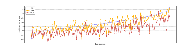
Figure 6: Group sufficiency gap on the specific subgroup $A=a$, which is the gap between $\mathbb{E}[Y|f(X)]$ and $\mathbb{E}[Y|f(X),A=a]$. We visualize the results for the entire users of Amazon Review dataset.

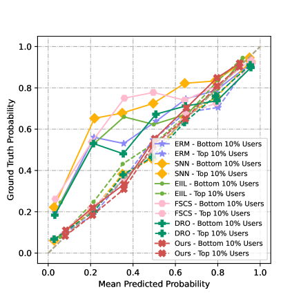
Figure 7: Probability calibration over aggregated users of Amazon Review dataset, where we sort the group sufficiency gap for each subgroup $A=a$, then we visualize the probability calibration curve for the top $10\%$ and bottom $10\%$ users. Since each user has quite limited labels, we aggregate the top $10\%$ and bottom $10\%$ and visualize the probability calibration. The results depict consistently better probability calibration of the proposed approach.

Appendix I Additional Results in Toxic Comments

I.1 Race as sensitive attribute: probability calibration

The additional results of the probability calibration on the Toxic Comments (Race) dataset is shown in Fig. 8.

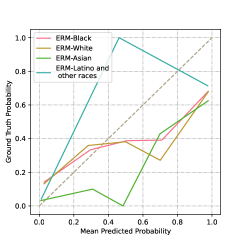
(a) ERM

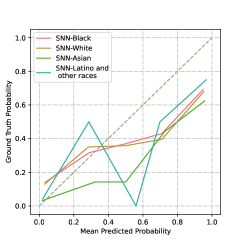
(b) SNN

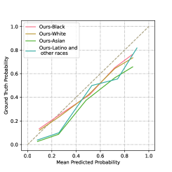
(c) Ours

Figure 8: Ablation. Results in Toxic dataset (Race). Visualization of probability calibration for each subgroup $A=a$, i.e. $(f(X),\mathbb{E}[Y|f(X),A=a])$. The proposed approach shows significant improved probability calibration for each subgroup.

I.2 Religion as sensitive attribute

The additional results of each subgroup’s fair performance and the probability calibration on the Toxic Comments (Religion) dataset are shown in Fig. 9 and Fig. 10.

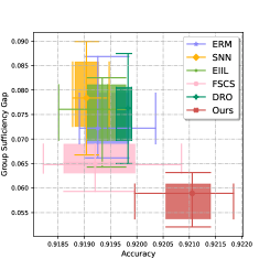
(a) Accuracy-$\textbf{Suf}_{f}$

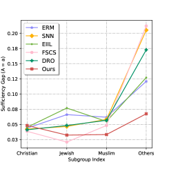
(b) $\textbf{Suf}_{f}$ on each subgroup

(c) Probability calibration

Figure 9: Results in Toxic dataset (Religion). Boxplot of accuracy and group sufficiency gap $\textbf{Suf}_{f}$ with 5 repeats: median, 75th percentile and minimum-maximum value. (b) Group sufficiency gap on the specific subgroup $A=a$, which is the gap between $\mathbb{E}[Y|f(X)]$ and $\mathbb{E}[Y|f(X),A=a]$. (c) Visualization of probability calibration over 5 repeats with mean and standard deviation. i.e $(f(X),\mathbb{E}[Y|f(X)])$.

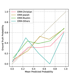
(a) ERM

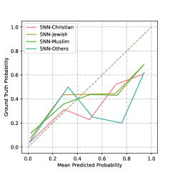
(b) SNN

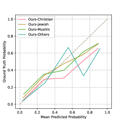
(c) Ours

Figure 10: Ablation. Results in Toxic dataset (Religion). Visualization of probability calibration for each subgroup $A=a$, i.e. $(f(X),\mathbb{E}[Y|f(X),A=a])$. The proposed approach shows significant improved probability calibration for each subgroup.

I.3 Gender as sensitive attribute

The additional results of each subgroup’s fair performance and the probability calibration on the Toxic Comments (Gender) dataset are shown in Fig. 11 and Fig. 12.

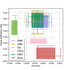
(a) Accuracy-$\textbf{Suf}_{f}$

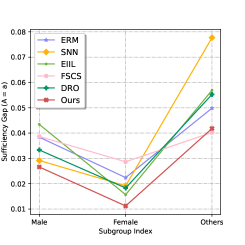
(b) $\textbf{Suf}_{f}$ on each subgroup

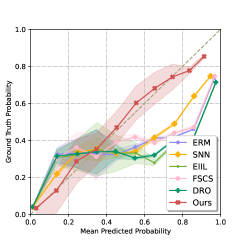
(c) Probability calibration

Figure 11: Results in Toxic dataset (Gender). Boxplot of accuracy and group sufficiency gap $\textbf{Suf}_{f}$ with 5 repeats: median, 75th percentile and minimum-maximum value. (b) Group sufficiency gap on the specific subgroup $A=a$, which is the gap between $\mathbb{E}[Y|f(X)]$ and $\mathbb{E}[Y|f(X),A=a]$. (c) Visualization of probability calibration over 5 repeats with mean and standard deviation. i.e $(f(X),\mathbb{E}[Y|f(X)])$.

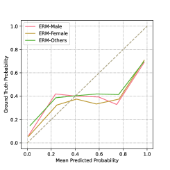
(a) ERM

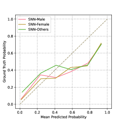
(b) SNN

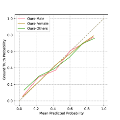
(c) Ours

Figure 12: Ablation. Results in Toxic dataset (Gender). Visualization of probability calibration for each subgroup $A=a$, i.e. $(f(X),\mathbb{E}[Y|f(X),A=a])$. The proposed approach shows significant improved probability calibration for each subgroup.

It is worth noting that although the group sufficiency in three approaches is quite similar. However, the proposed approach shows a significant better probability calibration than baselines.

I.4 Results on different subgroup numbers

We visualize the results on different subgroup numbers, shown in Fig. 13. The results still suggest the consistently better results than baselines.

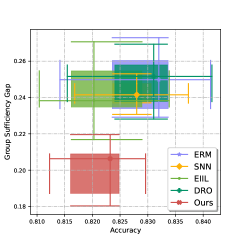
(a) Subgroup Number: 50

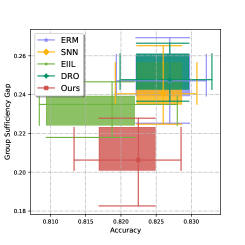
(b) Subgroup Number: 100

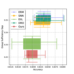
(c) Subgroup Number: 300

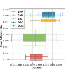
(d) Subgroup Number: 400

Figure 13: Results of different subgroups numbers on Amazon Review Dataset

I.5 Additional Results on Adult dataset

We further evaluated the Adult dataset [62], which predicts salary being larger than 50K or not. We treat gender as the sensitive attribute and subsample 500 samples for each subgroup. We adopt $\tilde{f}_{\bf{w}}$ and $\tilde{f}_{\bf{w}_{a}}$ as the two-layer fully connected neural network, where ${\bf w}\sim Q$ and ${\bf w}_{a}\sim Q_{a}$. All results are repeated 4 times and illustrated in Tab. 1.

Table 1: Results (average and std) in Adult dataset (on %)

Method	Accuracy	Group sufficiency gap (smaller is better)
ERM	83.38 (0.421)	1.096 (0.182)
SNN	82.62 (0.478)	1.071 (0.220)
EIIL	83.27 (0.547)	1.018 (0.239)
FSCS	83.63 (0.704)	1.271 (0.316)
DRO	83.48 (0.377)	1.056 (0.151)
Ours	83.33 (0.308)	0.684 (0.008)

The result suggests a consistently better group sufficiency with comparable accuracy.

I.6 Additional Results on vision dataset

We further consider CelebA dataset as a computer vision task [63]. We follow the protocol of [64], which predicts the wavy hair $Y$ in the image $X$. We regard gender as sensitive attribute $A$. We further adopted Res18 as the backbone and three layers fully-connected (randomized) layers. We sub-sample 200 instances per subgroup and fine tune for maximum 20 epochs. All results are repeated 4 times and illustrated in Tab. 2.

Table 2: Results (average and std) in CelebA dataset (on %)

Method	Accuracy	Group sufficiency gap (smaller is better)
ERM	79.67 (0.40)	7.13 (0.96)
SNN	79.79 (0.33)	7.12 (0.89)
EIIL	79.90 (0.30)	6.23 (1.52)
FSCS	79.33 (0.62)	7.01 (1.88)
DRO	79.82 (0.27)	6.68 (1.14)
Ours	79.87 (0.17)	5.29 (0.67)

The result also suggests a consistently better group sufficiency with comparable accuracy.

I.7 Evolution of Q during the training

We visualize the test accuracy and group sufficiency gap of fair predictor $Q$ during the training, shown in Tab. 3. The results are evaluated on the Toxic data with race as the sensitive attribute.

Table 3: Evolution of accuracy and group sufficiency gap during the training (on %)

Epoch	0	2	4	6	8	10	12	14
Suf gap	12.49	14.65	11.60	7.32	6.19	5.41	5.45	5.42
Accuracy	50.94	66.30	87.87	91.71	92.10	92.10	92.16	92.13

References

- Barocas et al. [2019] Solon Barocas, Moritz Hardt, and Arvind Narayanan. Fairness and Machine Learning. fairmlbook.org, 2019. http://www.fairmlbook.org.
- Kearns et al. [2018] Michael Kearns, Seth Neel, Aaron Roth, and Zhiwei Steven Wu. Preventing fairness gerrymandering: Auditing and learning for subgroup fairness. In International Conference on Machine Learning, pages 2564–2572. PMLR, 2018.
- Donini et al. [2018] Michele Donini, Luca Oneto, Shai Ben-David, John Shawe-Taylor, and Massimiliano Pontil. Empirical risk minimization under fairness constraints. arXiv preprint arXiv:1802.08626, 2018.
- Chouldechova [2017] Alexandra Chouldechova. Fair prediction with disparate impact: A study of bias in recidivism prediction instruments. Big data, 5(2):153–163, 2017.
- Vyas et al. [2020] Darshali A. Vyas, Leo G. Eisenstein, and David S. Jones. Hidden in plain sight — reconsidering the use of race correction in clinical algorithms. New England Journal of Medicine, 383(9):874–882, 2020. doi: 10.1056/NEJMms2004740. URL https://doi.org/10.1056/NEJMms2004740.
- Obermeyer et al. [2019] Ziad Obermeyer, Brian Powers, Christine Vogeli, and Sendhil Mullainathan. Dissecting racial bias in an algorithm used to manage the health of populations. Science, 366(6464):447–453, 2019. doi: 10.1126/science.aax2342. URL https://www.science.org/doi/abs/10.1126/science.aax2342.
- van Praat [2020] Frank van Praat. So, here’s the problem with self-driving cars. 2020.
- Subramanian et al. [2021] Shivashankar Subramanian, Afshin Rahimi, Timothy Baldwin, Trevor Cohn, and Lea Frermann. Fairness-aware class imbalanced learning. In Proceedings of the 2021 Conference on Empirical Methods in Natural Language Processing, pages 2045–2051, 2021. doi: 10.18653/v1/2021.emnlp-main.155. URL https://aclanthology.org/2021.emnlp-main.155.
- Chalkidis et al. [2022] Ilias Chalkidis, Tommaso Pasini, Sheng Zhang, Letizia Tomada, Sebastian Felix Schwemer, and Anders Søgaard. Fairlex: A multilingual benchmark for evaluating fairness in legal text processing. CoRR, abs/2203.07228, 2022.
- Gaut et al. [2020] Andrew Gaut, Tony Sun, Shirlyn Tang, Yuxin Huang, Jing Qian, Mai ElSherief, Jieyu Zhao, Diba Mirza, Elizabeth Belding, Kai-Wei Chang, and William Yang Wang. Towards understanding gender bias in relation extraction. In Proceedings of the 58th Annual Meeting of the Association for Computational Linguistics, pages 2943–2953, Online, 2020. Association for Computational Linguistics.
- Sheng et al. [2021] Emily Sheng, Kai-Wei Chang, Prem Natarajan, and Nanyun Peng. Societal biases in language generation: Progress and challenges. In Chengqing Zong, Fei Xia, Wenjie Li, and Roberto Navigli, editors, Proceedings of the 59th Annual Meeting of the Association for Computational Linguistics and the 11th International Joint Conference on Natural Language Processing, ACL/IJCNLP 2021, (Volume 1: Long Papers), Virtual Event, August 1-6, 2021, pages 4275–4293. Association for Computational Linguistics, 2021.
- Gupta et al. [2022] Umang Gupta, Jwala Dhamala, Varun Kumar, Apurv Verma, Yada Pruksachatkun, Satyapriya Krishna, Rahul Gupta, Kai-Wei Chang, Greg Ver Steeg, and Aram Galstyan. Mitigating gender bias in distilled language models via counterfactual role reversal. arXiv preprint arXiv:2203.12574, 2022.
- Saunders et al. [2021] Danielle Saunders, Rosie Sallis, and Bill Byrne. First the worst: Finding better gender translations during beam search. CoRR, abs/2104.07429, 2021.
- Jung et al. [2021] Sangwon Jung, Donggyu Lee, Taeeon Park, and Taesup Moon. Fair feature distillation for visual recognition. In IEEE Conference on Computer Vision and Pattern Recognition, CVPR 2021, virtual, June 19-25, 2021, pages 12115–12124. Computer Vision Foundation / IEEE, 2021.
- Li and Xu [2021] Zhiheng Li and Chenliang Xu. Discover the unknown biased attribute of an image classifier. In 2021 IEEE/CVF International Conference on Computer Vision, ICCV 2021, Montreal, QC, Canada, October 10-17, 2021, pages 14950–14959. IEEE, 2021. doi: 10.1109/ICCV48922.2021.01470. URL https://doi.org/10.1109/ICCV48922.2021.01470.
- Zhao et al. [2021] Dora Zhao, Angelina Wang, and Olga Russakovsky. Understanding and evaluating racial biases in image captioning. In 2021 IEEE/CVF International Conference on Computer Vision, ICCV 2021, Montreal, QC, Canada, October 10-17, 2021, pages 14810–14820. IEEE, 2021.
- Vu et al. [2020] Xuan-Son Vu, Thanh-Son Nguyen, Duc-Trong Le, and Lili Jiang. Multimodal review generation with privacy and fairness awareness. In Donia Scott, Núria Bel, and Chengqing Zong, editors, Proceedings of the 28th International Conference on Computational Linguistics, COLING 2020, Barcelona, Spain (Online), December 8-13, 2020, pages 414–425. International Committee on Computational Linguistics, 2020.
- Hardt et al. [2016] Moritz Hardt, Eric Price, and Nati Srebro. Equality of opportunity in supervised learning. Advances in neural information processing systems, 29:3315–3323, 2016.
- Zemel et al. [2013] Rich Zemel, Yu Wu, Kevin Swersky, Toni Pitassi, and Cynthia Dwork. Learning fair representations. In International conference on machine learning, pages 325–333. PMLR, 2013.
- Verma and Rubin [2018] Sahil Verma and Julia Rubin. Fairness definitions explained. In 2018 ieee/acm international workshop on software fairness (fairware), pages 1–7. IEEE, 2018.
- Jiang et al. [2020] Ray Jiang, Aldo Pacchiano, Tom Stepleton, Heinrich Jiang, and Silvia Chiappa. Wasserstein fair classification. In Uncertainty in Artificial Intelligence, pages 862–872. PMLR, 2020.
- Feldman [2015] Michael Feldman. Computational fairness: Preventing machine-learned discrimination. PhD thesis, 2015.
- Calmon et al. [2017] Flavio P Calmon, Dennis Wei, Bhanukiran Vinzamuri, Karthikeyan Natesan Ramamurthy, and Kush R Varshney. Optimized pre-processing for discrimination prevention. In Proceedings of the 31st International Conference on Neural Information Processing Systems, pages 3995–4004, 2017.
- Sagawa* et al. [2020] Shiori Sagawa*, Pang Wei Koh*, Tatsunori B. Hashimoto, and Percy Liang. Distributionally robust neural networks. In International Conference on Learning Representations, 2020. URL https://openreview.net/forum?id=ryxGuJrFvS.
- Zhao et al. [2019] Han Zhao, Amanda Coston, Tameem Adel, and Geoffrey J Gordon. Conditional learning of fair representations. arXiv preprint arXiv:1910.07162, 2019.
- Li et al. [2019] Tian Li, Maziar Sanjabi, Ahmad Beirami, and Virginia Smith. Fair resource allocation in federated learning. arXiv preprint arXiv:1905.10497, 2019.
- Li et al. [2021] Tian Li, Shengyuan Hu, Ahmad Beirami, and Virginia Smith. Ditto: Fair and robust federated learning through personalization. In International Conference on Machine Learning, pages 6357–6368. PMLR, 2021.
- Hashimoto et al. [2018] Tatsunori Hashimoto, Megha Srivastava, Hongseok Namkoong, and Percy Liang. Fairness without demographics in repeated loss minimization. In International Conference on Machine Learning, pages 1929–1938. PMLR, 2018.
- Martinez et al. [2019] Natalia Martinez, Martin Bertran, and Guillermo Sapiro. Fairness with minimal harm: A pareto-optimal approach for healthcare. arXiv preprint arXiv:1911.06935, 2019.
- Balashankar et al. [2019] Ananth Balashankar, Alyssa Lees, Chris Welty, and Lakshminarayanan Subramanian. What is fair? exploring pareto-efficiency for fairness constrained classifiers. arXiv preprint arXiv:1910.14120, 2019.
- Zafar et al. [2019] Muhammad Bilal Zafar, Isabel Valera, Manuel Gomez-Rodriguez, and Krishna P Gummadi. Fairness constraints: A flexible approach for fair classification. The Journal of Machine Learning Research, 20(1):2737–2778, 2019.
- Song et al. [2019] Jiaming Song, Pratyusha Kalluri, Aditya Grover, Shengjia Zhao, and Stefano Ermon. Learning controllable fair representations. In The 22nd International Conference on Artificial Intelligence and Statistics, pages 2164–2173. PMLR, 2019.
- Madras et al. [2018] David Madras, Elliot Creager, Toniann Pitassi, and Richard Zemel. Learning adversarially fair and transferable representations. In International Conference on Machine Learning, pages 3384–3393. PMLR, 2018.
- Huang and Vishnoi [2019] Lingxiao Huang and Nisheeth Vishnoi. Stable and fair classification. In International Conference on Machine Learning, pages 2879–2890. PMLR, 2019.
- Dutta et al. [2020] Sanghamitra Dutta, Dennis Wei, Hazar Yueksel, Pin-Yu Chen, Sijia Liu, and Kush Varshney. Is there a trade-off between fairness and accuracy? a perspective using mismatched hypothesis testing. In International Conference on Machine Learning, pages 2803–2813. PMLR, 2020.
- Wang et al. [2021] Yuyan Wang, Xuezhi Wang, Alex Beutel, Flavien Prost, Jilin Chen, and Ed H Chi. Understanding and improving fairness-accuracy trade-offs in multi-task learning. arXiv preprint arXiv:2106.02705, 2021.
- Pleiss et al. [2017] Geoff Pleiss, Manish Raghavan, Felix Wu, Jon Kleinberg, and Kilian Q Weinberger. On fairness and calibration. arXiv preprint arXiv:1709.02012, 2017.
- Liu et al. [2019] Lydia T. Liu, Max Simchowitz, and Moritz Hardt. The implicit fairness criterion of unconstrained learning. In Kamalika Chaudhuri and Ruslan Salakhutdinov, editors, Proceedings of the 36th International Conference on Machine Learning, volume 97 of Proceedings of Machine Learning Research, pages 4051–4060. PMLR, 09–15 Jun 2019. URL https://proceedings.mlr.press/v97/liu19f.html.
- Shui et al. [2022a] Changjian Shui, Qi Chen, Jiaqi Li, Boyu Wang, and Christian Gagné. Fair representation learning through implicit path alignment. In ICML, 2022a.
- Koh et al. [2021] Pang Wei Koh, Shiori Sagawa, Henrik Marklund, Sang Michael Xie, Marvin Zhang, Akshay Balsubramani, Weihua Hu, Michihiro Yasunaga, Richard Lanas Phillips, Irena Gao, et al. Wilds: A benchmark of in-the-wild distribution shifts. In International Conference on Machine Learning, pages 5637–5664. PMLR, 2021.
- Lee et al. [2021] Joshua K Lee, Yuheng Bu, Deepta Rajan, Prasanna Sattigeri, Rameswar Panda, Subhro Das, and Gregory W Wornell. Fair selective classification via sufficiency. In International Conference on Machine Learning, pages 6076–6086. PMLR, 2021.
- Guo et al. [2017] Chuan Guo, Geoff Pleiss, Yu Sun, and Kilian Q Weinberger. On calibration of modern neural networks. In International Conference on Machine Learning, pages 1321–1330. PMLR, 2017.
- Creager et al. [2021] Elliot Creager, Jörn-Henrik Jacobsen, and Richard Zemel. Environment inference for invariant learning. In International Conference on Machine Learning, pages 2189–2200. PMLR, 2021.
- Liu et al. [2021] Risheng Liu, Jiaxin Gao, Jin Zhang, Deyu Meng, and Zhouchen Lin. Investigating bi-level optimization for learning and vision from a unified perspective: A survey and beyond. IEEE Transactions on Pattern Analysis and Machine Intelligence, pages 1–1, 2021. doi: 10.1109/TPAMI.2021.3132674.
- Raghavan et al. [2020] Manish Raghavan, Solon Barocas, Jon Kleinberg, and Karen Levy. Mitigating bias in algorithmic hiring: Evaluating claims and practices. In Proceedings of the 2020 conference on fairness, accountability, and transparency, pages 469–481, 2020.
- Baydin et al. [2018] Atilim Gunes Baydin, Barak A. Pearlmutter, Alexey Andreyevich Radul, and Jeffrey Mark Siskind. Automatic differentiation in machine learning: a survey. Journal of Machine Learning Research, 18(153):1–43, 2018. URL http://jmlr.org/papers/v18/17-468.html.
- Park and Oliva [2019] Eunbyung Park and Junier B Oliva. Meta-curvature. Advances in Neural Information Processing Systems, 32, 2019.
- Shui et al. [2022b] Changjian Shui, Qi Chen, Jiaqi Li, Boyu Wang, and Christian Gagné. Fair representation learning through implicit path alignment. arXiv preprint arXiv:2205.13316, 2022b.
- Shalev-Shwartz and Ben-David [2014] Shai Shalev-Shwartz and Shai Ben-David. Understanding machine learning: From theory to algorithms. Cambridge university press, 2014.
- Pentina and Lampert [2014] Anastasia Pentina and Christoph Lampert. A pac-bayesian bound for lifelong learning. In International Conference on Machine Learning, pages 991–999. PMLR, 2014.
- Amit and Meir [2018] Ron Amit and Ron Meir. Meta-learning by adjusting priors based on extended pac-bayes theory. In International Conference on Machine Learning, pages 205–214. PMLR, 2018.
- CHEN et al. [2021] Qi CHEN, Changjian Shui, and Mario Marchand. Generalization bounds for meta-learning: An information-theoretic analysis. In A. Beygelzimer, Y. Dauphin, P. Liang, and J. Wortman Vaughan, editors, Advances in Neural Information Processing Systems, 2021. URL https://openreview.net/forum?id=9J2wV5E1Aq_.
- Kingma and Welling [2013] Diederik P Kingma and Max Welling. Auto-encoding variational bayes. arXiv preprint arXiv:1312.6114, 2013.
- Blundell et al. [2015] Charles Blundell, Julien Cornebise, Koray Kavukcuoglu, and Daan Wierstra. Weight uncertainty in neural network. In International Conference on Machine Learning, pages 1613–1622. PMLR, 2015.
- Ni et al. [2019] Jianmo Ni, Jiacheng Li, and Julian McAuley. Justifying recommendations using distantly-labeled reviews and fine-grained aspects. In Proceedings of the 2019 Conference on Empirical Methods in Natural Language Processing and the 9th International Joint Conference on Natural Language Processing (EMNLP-IJCNLP), pages 188–197, 2019.
- Koenecke et al. [2020] Allison Koenecke, Andrew Nam, Emily Lake, Joe Nudell, Minnie Quartey, Zion Mengesha, Connor Toups, John R Rickford, Dan Jurafsky, and Sharad Goel. Racial disparities in automated speech recognition. Proceedings of the National Academy of Sciences, 117(14):7684–7689, 2020.
- Sanh et al. [2019] Victor Sanh, Lysandre Debut, Julien Chaumond, and Thomas Wolf. Distilbert, a distilled version of bert: smaller, faster, cheaper and lighter. arXiv preprint arXiv:1910.01108, 2019.
- Borkan et al. [2019] Daniel Borkan, Lucas Dixon, Jeffrey Sorensen, Nithum Thain, and Lucy Vasserman. Nuanced metrics for measuring unintended bias with real data for text classification. In Companion proceedings of the 2019 world wide web conference, pages 491–500, 2019.
- Bishop [2006] Christopher M. Bishop. Pattern Recognition and Machine Learning. Springer, 2006.
- Wainwright [2019] Martin J Wainwright. High-dimensional statistics: A non-asymptotic viewpoint, volume 48. Cambridge University Press, 2019.
- Hu et al. [2021] Hongsheng Hu, Zoran Salcic, Gillian Dobbie, and Xuyun Zhang. Membership inference attacks on machine learning: A survey. arXiv preprint arXiv:2103.07853, 2021.
- Dua and Graff [2017] Dheeru Dua and Casey Graff. UCI machine learning repository, 2017. URL http://archive.ics.uci.edu/ml.
- Liu et al. [2015] Ziwei Liu, Ping Luo, Xiaogang Wang, and Xiaoou Tang. Deep learning face attributes in the wild. In Proceedings of International Conference on Computer Vision (ICCV), December 2015.
- Chuang and Mroueh [2021] Ching-Yao Chuang and Youssef Mroueh. Fair mixup: Fairness via interpolation. arXiv preprint arXiv:2103.06503, 2021.