A Unified Neural Network Model for Readability Assessment
with Feature Projection and Length-Balanced Loss
Abstract
For readability assessment, traditional methods mainly employ machine learning classifiers with hundreds of linguistic features. Although the deep learning model has become the prominent approach for almost all NLP tasks, it is less explored for readability assessment. In this paper, we propose a BERT-based model with feature projection and length-balanced loss (BERT-FP-LBL) for readability assessment. Specially, we present a new difficulty knowledge guided semi-supervised method to extract topic features to complement the traditional linguistic features. From the linguistic features, we employ projection filtering to extract orthogonal features to supplement BERT representations. Furthermore, we design a new length-balanced loss to handle the greatly varying length distribution of data. Our model achieves state-of-the-art performances on two English benchmark datasets and one dataset of Chinese textbooks, and also achieves the near-perfect accuracy of 99% on one English dataset. Moreover, our proposed model obtains comparable results with human experts in consistency test.
1 Introduction
Readability assessment is to automatically determine the difficulty level of a given text, aiming to recommend suitable reading materials to readers. There are wide applications of readability assessment, such as automating readers’ advisory Pera and Ng (2014), clinical informed consent forms Perni et al. (2019) and internet-based patient education materials Sare et al. (2020).
Comparing with other natural language processing (NLP) tasks, readability assessment is less explored. In the early days, researchers exploit linguistic features to develop various readability formulas, such as Flesch Flesch (1948), Dale-Chall Dale and Chall (1948) and SMOG Mc Laughlin (1969). Later, the mainstream research Deutsch et al. (2020); Hansen et al. (2021); Lee et al. (2021) is to employ machine learning models to classify a text, by designing a large number of linguistic features. There are also works that treat it as a regression task Sheehan et al. (2010) or a ranking task Lee and Vajjala (2022).
Recently, unlike other NLP tasks, the introduction of deep neural networks for readability assessment does not achieve overwhelming advantages over traditional machine learning methods. Employing neural network models for readability assessment, there are several challenges:
(1) The scale of the dataset for readability assessment is small, which restricts the performance of deep neural network models.
(2) The deep neural network model is mainly based on characters or words and the extracted features are often at a shallow level. As a result, words with similar functions or meanings, such as “man” and “gentleman”, are mapped into close vectors although their reading difficulties are different Jiang et al. (2018).
(3) The linguistic features designed by researchers and continuous features extracted by neural network models are from two different semantic spaces. If two kinds of features are simply concatenated, it will bring redundant information or even harmful effects to model performance.
(4) Unlike other NLP data whose length follows a normal distribution, a notable problem with the data for readability assessment is that the text length varies greatly. The texts with low difficulty are usually shorter, while texts with high difficulty are usually longer. For example, as shown in Table 1, in ChineseLR the average length of Level 1 is only 266 characters, while the average length of Level 5 is 3,299 characters. As a result, when experimented with deep learning networks, shorter texts tend to converge much faster than those longer ones thus harm the overall performance.
In order to solve the above problems, we propose a BERT-based model with Feature Projection and Length-Balanced Loss (BERT-FP-LBL). With the pre-trained BERT as the backbone, we employ feature projection to integrate linguistic features into the neural model, and design a new length-balanced loss function to guide the training. Concretely:
-
•
We leverage BERT and a mixed-pooling mechanism to obtain text representations, which take advantage of the powerful representative ability of pre-trained model, and thus overcome the data-sparsity problem.
-
•
Beyond traditional features, we extract a set of topic features enriched with difficulty knowledge, which are high-level global features. Specifically, based on a graded lexicon, we exploit a clustering algorithm to group related words belonging to the same difficulty level, which then serve as anchor words to guide the training of a semi-supervised topic model.
-
•
Rather than simple concatenation, we project linguistic features to the neural network features to obtain orthogonal features, which supplement the neural network representations.
-
•
We introduce a new length-balanced loss function to revise the standard cross entropy loss, which balances the varying length distribution of data for readability assessment.
We conduct experiments on three English benchmark datasets, including WeeBit Vajjala and Meurers (2012), OneStopEnglish Vajjala and Lučić (2018) and Cambridge Xia et al. (2019), and one Chinese dataset collected from school textbooks. Experimental results show that our proposed model outperforms the baseline model by a wide margin, and achieves new state-of-the-art results on WeeBit and Cambridge.
We also conduct test to measure the correlation coefficient between the BERT-FP-LBL model’s inference results and three human experts, and the results demonstrate that our model achieves comparable results with human experts. We will make our code public available, and release our Chinese feature extraction toolkit zhfeat 111https://github.com/liwb1219/zhfeat.
2 Related Work
Traditional Methods. Early research efforts focused on various linguistic features as defined by linguists. Researchers use these features to create various formulas for readability, including Flesch Flesch (1948), Dale-Chall Dale and Chall (1948) and SMOG Mc Laughlin (1969). Although the readability formula has the advantages of simplicity and objectivity, there are also some problems, such as the introduction of fewer variables during the development, and insufficient consideration of the variables at the discourse level.
Machine Learning Classification Methods. Schwarm and Ostendorf (2005) develop a method of reading level assessment that uses support vector machines (SVMs) to combine features from statistical language models (LMs), parse trees, and other traditional features used in reading level assessment. Subsequently, Petersen and Ostendorf (2009) present expanded results for the SVM detectors. Qiu et al. (2017) designe 100 factors to systematically evaluate the impact of four levels of linguistic features (shallow, POS, syntactic, discourse) on predicting text difficulty for L1 Chinese learners and further selected 22 significant features with regression. Lu et al. (2019) design experiments to analyze the influence of 88 linguistic features on sentence complexity and results suggest that the linguistic features can significantly improve the predictive performance with the highest of 70.78% distance-1 adjacent accuracy. Deutsch et al. (2020); Lee et al. (2021) evaluate the joint application of handcrafted linguistic features and deep neural network models. The handcrafted linguistic features are fused with the features of neural networks and fed into a machine learning model for classification.
Neural Network Models. Jiang et al. (2018) provide the knowledge-enriched word embedding (KEWE) for readability assessment, which encodes the knowledge on reading difficulty into the representation of words. Azpiazu and Pera (2019) present a multi-attentive recurrent neural network architecture for automatic multilingual readability assessment. This architecture considers raw words as its main input, but internally captures text structure and informs its word attention process using other syntax and morphology-related datapoints, known to be of great importance to readability. Meng et al. (2020) propose a new and comprehensive framework which uses a hierarchical self-attention model to analyze document readability. Qiu et al. (2021) form a correlation graph among features, which represent pairwise correlations between features as triplets with linguistic features as nodes and their correlations as edges.
3 Methodology
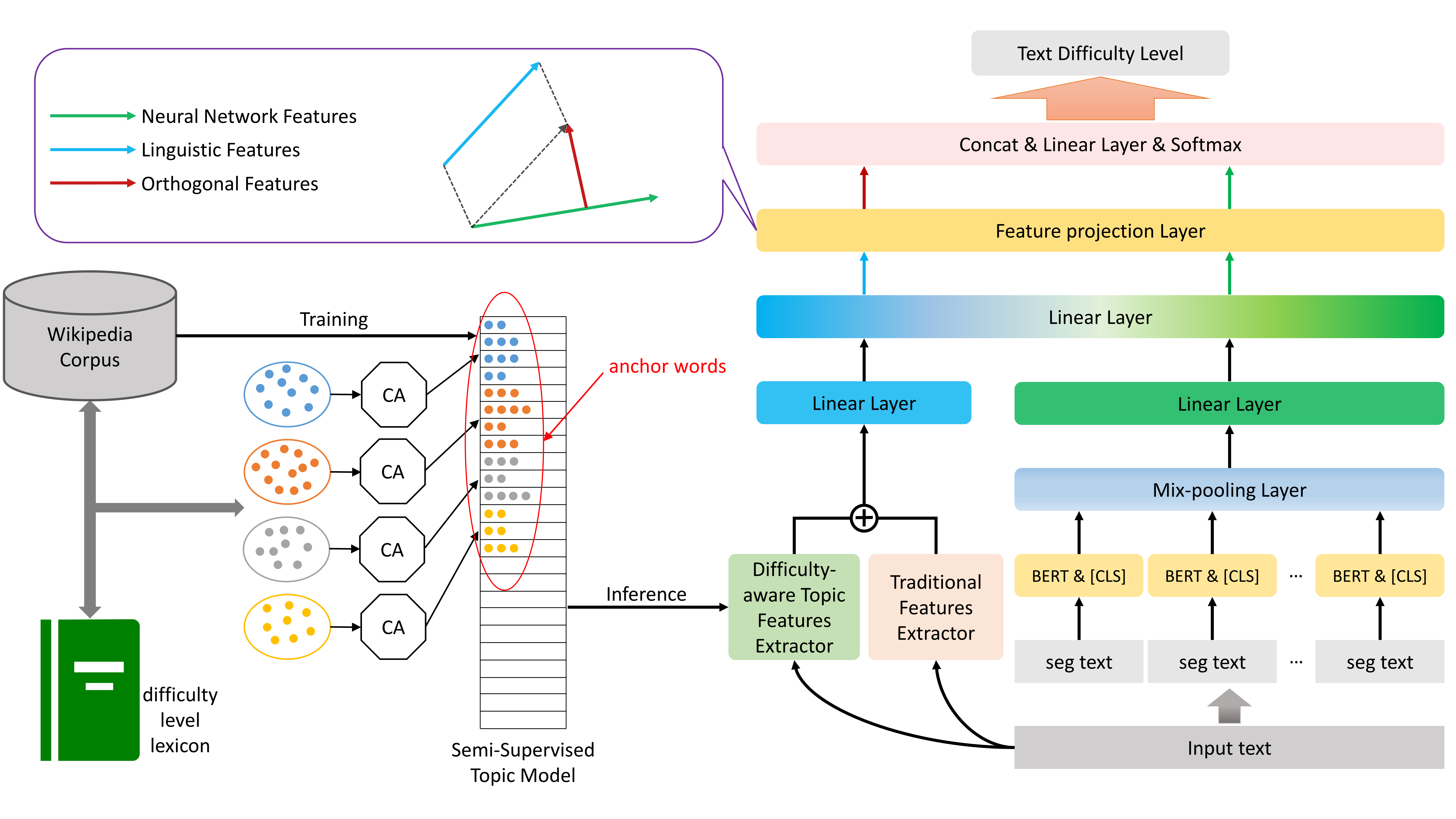
The overall structure of our model is illustrated in Figure 1. We integrate difficulty knowledge to extract topic features using the Anchored Correlation Explanation (CorEx) Gallagher et al. (2017), and fuse linguistic features with neural network representations through projection filtering. Further, we propose a new length-balanced loss function to deal with the unbalanced length distribution of the readability assessment data.
3.1 Traditional Features
Many previous studies have proved that shallow and linguistic features are helpful for readability assessment. For Chinese traditional features, we develop a Chinese toolkit zhfeat to extract character, word, sentence and paragraph features. Please refer to Appendix A for detailed descriptions. For English traditional features, we extract discourse, syntactic, lexical and shallow features, by directly implementing the lingfeat Lee et al. (2021) toolkit. We denote the traditional features as .
3.2 Topic Features with Difficulty Knowledge
Background. Besides the above lexical and syntactic features, topic features provide high-level semantic information for assessing difficulty level. Lee et al. (2021) also leverage topic features, but they train the topic model in a purely unsupervised way without considering difficulty knowledge. Inspired by the work of Anchored Correlation Explanation (CorEx) Gallagher et al. (2017), which allows integrating domain knowledge through anchor words, we introduce word difficulty knowledge to guide the training of topic model, thus obtaining difficulty-aware topic features.
First, we introduce the concept of information bottleneck Tishby et al. (2000), which aims to achieve a trade-off between compressing feature into representation and preserving as much information as possible with respect to the label . Formally, the information bottleneck is expressed as:
| (1) |
| (2) | ||||
where is the mutual information of random variables and , represents the entropy of the random variable , and represents the Lagrange multiplier.
In CorEx, if we want to learn representations that are more relevant to specific keywords, we can anchor a word type to topic , and control the strength of anchoring by constraining optimization . The optimization objective is:
| (3) |
where represents the number of topics, is the number of words corresponding to the topic, and represents the anchoring strength of the word to the topic .
Extracting difficulty-aware Topic Features. We utilize a lexicon containing words of varying difficulty levels to extract anchor words. Let be a graded lexicon, where is the set of words with difficulty level . is the corpus for pre-training the topic model. First, we select out some high frequent words of each level in the corpus :
| (4) |
where represents the intersection operation.
For each level of words, we conduct KMeans clustering algorithm to do classification, and then remove isolated word categories (a single word is categorized as a class):
| (5) |
The clustering result of words with the difficulty level is denoted as . Thus, the final anchor words are:
| (6) |
These anchor words of different difficulty levels serve as domain knowledge to guide the training of topic models:
| (7) |
where ATM represents the anchored topic model. Then, we implement the ATM to obtain a set of topic distribution features involving difficulty information, which are denoted as .
Combining traditional and topic features, we obtain the overall linguistic features:
| (8) |
where represents the splicing operation.
3.3 Feature Fusion with Projection Filtering
BERT Representation. We leverage the pre-trained BERT model Devlin et al. (2018) to obtain sentence representation.
The length distribution of data for readability evaluation varies greatly, and texts with higher difficulty are very long, which might exceed the input limit of the model. Therefore, for an input text , we segment it as . For each segment, we exploit BERT to extract its semantic representation: .
Further, we adopt Mixed Pooling Yu et al. (2014) to extract representations of the entire text:
| (9) | ||||
where is a parameter to balance the ratio between max pooling and mean pooling.
Projection Filtering. To obtain better performance, we try to combine BERT representations with linguistic features. As for the method of direct splicing, since two kinds of features come from different semantic spaces, not only will it introduce some repetitive information, but also it may bring contradictions between some features that will harm the performance. When performing feature fusion, our goal is to obtain additional orthogonal features to complement each other. Inspired by the work Qin et al. (2020), which uses two identical encoders with different optimization objectives to extract common and differentiated features. Unlike this work, our artificial features and neural features are extracted in different ways, and our purpose is to perform feature complementation. Since the pre-trained model captures more semantic-level features through the contextual co-occurrence relationship between large-scale corpora. This is not enough for readability tasks, and the discrimination of difficulty requires some supplementary features (difficulty, syntax, etc.). So we consider the features extracted by BERT as primary features and linguistic features as secondary ones, and then the secondary features are projected into the primary features to obtain additional orthogonal features.
Concretely, based on the linguistic features and BERT representation , we perform dimensional transformation and project them into the same vector space:
| (10) |
| (11) |
where , and are the trainable parameters, and , and are the scalar biases.
Next, we project the secondary features into primary ones to obtain additional orthogonal features :
| (12) |
The orthogonal features are further added to the BERT representation to constitute the final text representation:
| (13) |
Finally, we compute the probability that a text belongs to the category by:
| (14) |
where is the trainable parameters, and are scalar biases.
3.4 Length Balanced Loss Function
The text length is an important aspect for determining the reading difficulty level. As shown in Table 1, a text with high difficulty level generally contains more tokens than that of low level. For example, on Cambridge dataset, the average length of Level 1 is 141 tokens, while the average length of Level 5 is 751 tokens. When experimented with deep learning methods, texts with short length tend to converge much faster than the texts with long length that influences the final performance.
To address this issue, we revise the loss to handle varying length. Specially, we measure the length distribution by weighting different length attributes, including the average, median, minimum and maximum length:
| (15) |
where represents the length value of the text category , ,, and represent the average, median, minimum and maximum length of the text, respectively. is the total number of categories.
We normalize the length value to obtain the length coefficient for each category:
| (16) |
Accordingly, the final loss function for a single sample is defined as:
| (17) |
where is the true label of text, is the adjustment factor of length distribution. When , it is reduced to the traditional cross entropy loss.
| Dataset | WeeBit | OneStopE | Cambridge | ChineseLR | ||||
| Level | Passages | Avg.Length | Passages | Avg.Length | Passages | Avg.Length | Passages | Avg.Length |
| 1 | 625 | 152 | 189 | 535 | 60 | 141 | 814 | 266 |
| 2 | 625 | 189 | 189 | 678 | 60 | 271 | 1063 | 679 |
| 3 | 625 | 295 | 189 | 825 | 60 | 617 | 1104 | 1140 |
| 4 | 625 | 242 | 0 | 0 | 60 | 763 | 762 | 2165 |
| 5 | 625 | 347 | 0 | 0 | 60 | 751 | 417 | 3299 |
| All | 3125 | 245 | 567 | 679 | 300 | 509 | 4160 | 1255 |
4 Experimental Setup
4.1 Datasets
To demonstrate the effectiveness of our proposed method, we conduct experiments on three English datasets and one Chinese dataset. We split the train, valid and test data according to the ratio of 8:1:1. The statistic distribution of datasets can be found in Table 1.
WeeBit Vajjala and Meurers (2012) is often considered as the benchmark data for English readability assessment. It was originally created as an extension of the well-known Weekly Reader corpus. We downsample to 625 passages per class.
OneStopEnglish Vajjala and Lučić (2018) is an aligned channel corpus developed for readability assessment and simplification research. Each text is paraphrased into three versions.
Cambridge Xia et al. (2019) is a dataset consisting of reading passages from the five main suite Cambridge English Exams (KET, PET, FCE, CAE, CPE). We downsample to 60 passages per class.
ChineseLR. ChineseLR is a Chinese dataset that we collected from textbooks of middle and primary school of more than ten publishers. To suit our task, we delete poetry and traditional Chinese texts. Following the standards specified in the Chinese Curriculum Standards for Compulsory Education, we category all texts to five difficulty levels.
4.2 Baseline Models
SVM. We employ support vector machines as the traditional machine learning classifier. The input to the model is the linguistic feature . We adopt MinMaxScaler (ranging from -1 to 1) for linguistic features and use the RBF kernel function. We use the libsvm 222https://www.csie.ntu.edu.tw/~cjlin/libsvm/ framework for experiments.
BERT. We utilize in Equation 9 followed by a linear layer classifier as our BERT baseline model.
4.3 Training and Evaluation Details
For the selection of the difficulty level lexicon , on the English dataset, we use the lexicon released by Maddela and Xu (2018), where we only use the first 4 levels. On the Chinese dataset, we use the Compulsory Education Vocabulary Su (2019). The word embedding features of English and Chinese word clustering algorithms are respectively used Pennington et al. (2014) and Song et al. (2018). We use the Wikipedia corpus 333https://dumps.wikimedia.org/ for pre-training the semi-supervised topic models. Please refer to Appendix B for some other details.
We do experiments using the Pytorch Paszke et al. (2019) framework. For training, we use the AdamW optimizer, the weight decay is 0.02 and the warm-up ratio is 0.1. The mixing pooling ratio is set to 0.5. Other specific parameter settings are shown in Table 2.
For evaluation, we calculate the accuracy, weighted F1 score, precision, recall and quadratic weighted kappa (QWK). We repeated each experiment three times and reported the average score.
| Dataset | Batch | MaxLen | Epoch | lr | |
| WeeBit | 8 | 512 | 10 | 3e-5 | 0.8 |
| OneStopE | 8 | 500×2 | 10 | 3e-5 | 0.4 |
| Cambridge | 8 | 500×2 | 10 | 3e-5 | 0.6 |
| ChineseLR | 2 | 500×8 | 10 | 3e-5 | 0.4 |
| Dataset | Metrics | Qiu-2021 | Mar-2021 | Lee-2021 | SVM | BERT | BERT-FP-LBL |
| WeeBit | Accuracy | 87.32 | 85.73 | 90.50 | 79.37 | 91.11 | 92.70 |
| F1 | - | 85.81 | 90.50 | 79.27 | 91.07 | 92.73 | |
| Precision | - | 86.58 | 90.50 | 79.26 | 91.42 | 92.89 | |
| Recall | - | 85.73 | 90.40 | 79.37 | 91.11 | 92.70 | |
| QWK | - | 95.27 | 96.80 | 93.22 | 97.36 | 97.78 | |
| OneStopE | Accuracy | 86.61 | 78.72 | 99.00 | 89.47 | 97.66 | 99.42 |
| F1 | - | 78.88 | 99.50 | 89.32 | 97.66 | 99.41 | |
| Precision | - | 79.77 | 99.50 | 89.41 | 97.83 | 99.44 | |
| Recall | - | 78.72 | 99.60 | 89.47 | 97.66 | 99.42 | |
| QWK | - | 82.45 | 99.60 | 92.31 | 92.98 | 98.25 | |
| Cambridge | Accuracy | 78.52 | - | 76.30 | 83.33 | 82.22 | 87.78 |
| F1 | - | - | 75.20 | 83.45 | 81.97 | 87.73 | |
| Precision | - | - | 79.20 | 90.91 | 82.96 | 89.46 | |
| Recall | - | - | 75.30 | 83.33 | 82.22 | 87.78 | |
| QWK | - | - | 91.90 | 91.97 | 94.65 | 96.87 | |
| ChineseLR | Accuracy | - | - | - | 76.67 | 75.16 | 78.89 |
| F1 | - | - | - | 76.53 | 75.05 | 78.75 | |
| Precision | - | - | - | 76.47 | 75.95 | 79.43 | |
| Recall | - | - | - | 76.67 | 75.16 | 78.89 | |
| QWK | - | - | - | 90.60 | 90.40 | 91.63 |
5 Results and Analysis
5.1 Overall Results
The experimental results of all models are summarized in Table 3. First of all, it should be noted that there are only a few studies on readability assessment, and there is no unified standard for data division and experimental parameter configuration. This has led to large differences in the results of different research works.
Our BERT-FP-LBL model achieves consistent improvements over the baselines on all four datasets, which validates the effectiveness of our proposed method. In terms of F1 metrics, our method improves WeeBit and ChineseLR by 1.66 and 3.7 compared to the baseline BERT model. Overall, our model achieves state-of-the-art performance on WeeBit and Cambridge. On OneStopEnglish, our model also achieves competitive results compared to previous work Lee et al. (2021), also achieving near-perfect classification accuracy of 99%.
Comparing the experimental results of SVM and the base BERT, it can be observed that on Cambridge and ChineseLR, SVM outperforms BERT. We believe this benefits from the linguistic features of our design.
| Model | WeeBit | ChineseLR |
| BERT-FP-LBL | 92.73 | 78.75 |
| -AW | 92.42 | 78.23 |
| -TFDK | 92.12 | 77.48 |
| -FP | 92.25 | 78.27 |
| -LBL | 91.76 | 76.94 |
5.2 Ablation Study
To illustrate the contribution of each module in our model, we conduct ablation experiments on WeeBit and ChineseLR, and the results are reported in Table 4.
When AW is removed, the CorEx changes from semi-supervised to unsupervised. The F1 scores of WeeBit and ChineseLR drop by 0.31 and 0.52, respectively, and when TFDK is removed, the corresponding F1 scores drop by 0.61 and 1.27, respectively. This indicates that our topic features incorporating difficulty knowledge indeed contribute to readability assessment.
Furthermore, when FP is removed, as described in Section 3.3, the simple splice operation brings some duplication or even negative information to the model. The F1 scores of WeeBit and ChineseLR both drop by 0.48.
Finally, when LBL is removed, the F1 scores of WeeBit and ChineseLR drop by 0.97 and 1.81, respectively. We believe that the difference in the length distribution of the dataset affects the convergence speed of different categories, which in turn will have an impact on the results. Besides, the drop in F1 metric is much more severe on ChineseLR than on WeeBit, and this result can be attributed to the more severe length imbalance on ChineseLR as shown in Table 1.
5.3 Analysis on the Length-balanced Loss
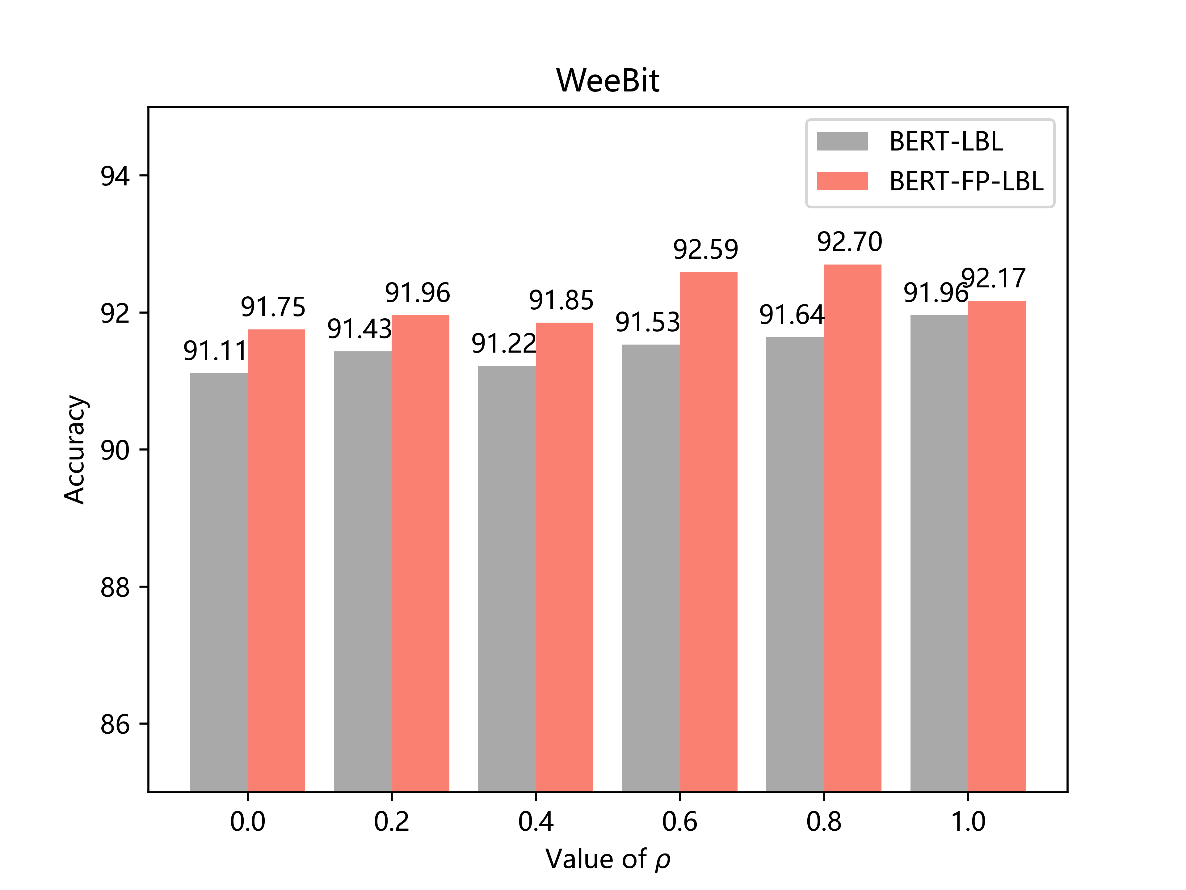
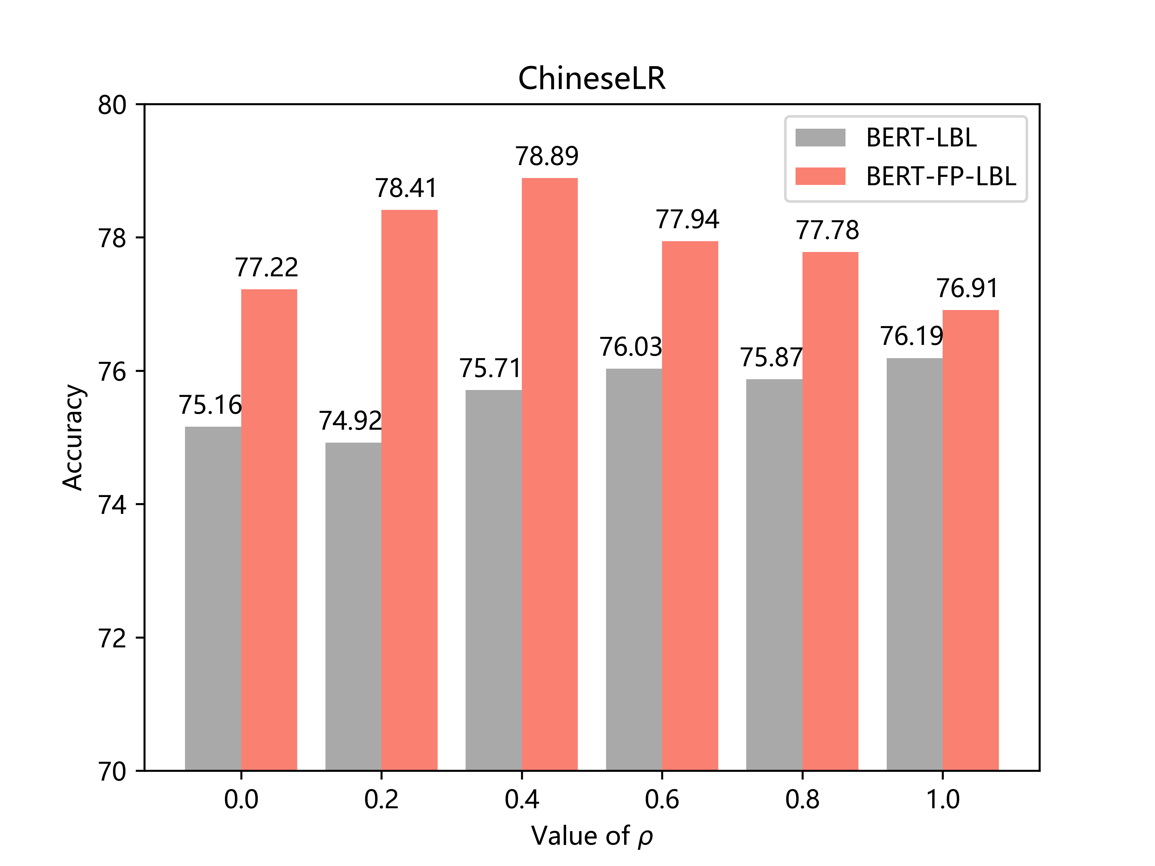
To explore the effect of length-balanced loss, we set different to conduct experiments. The larger the is, the difference between the loss of different categories is bigger. The loss difference leads to different convergence rates. When is 0, the loss function is the standard cross entropy loss, and there is no difference in the loss contributed by different categories. The specific results are shown in Figure 2.
For BERT, the optimal value of is relatively large, which means the model needs a relatively big difference in the loss to solve the problem of unbalanced text length. This indicates that there are indeed differences in the convergence speed between different classes, and this difference can be reduced by correcting the loss contributed by different classes. After adding orthogonal features, the optimal value of is relatively small. We think that whether the text is short or long, the number of parameters of its corresponding orthogonal features is fixed and does not require the length-balanced loss to adjust. So, when BERT features are combined with orthogonal features, the optimal value of will be lower than that in BERT alone.
In addition, the optimal value of on WeeBit is 0.8, while the optimal value of on ChineseLR is 0.4. This is perhaps because the WeeBit dataset has a small span of length distribution (maximum 512 truncation), and we need to relatively amplify the differences between different categories. However, the length distribution of the ChineseLR dataset has a large span (500×8), and we need to relatively narrow the differences between different categories.
Of course, the optimal value of is related to the specific data distribution, which is a parameter that needs to grid search. Generally speaking, when the length difference between different categories is small, we set relatively large, and when the length difference between different categories is large, we set relatively small.
5.4 Analysis on the Difficulty-aware Topic Features
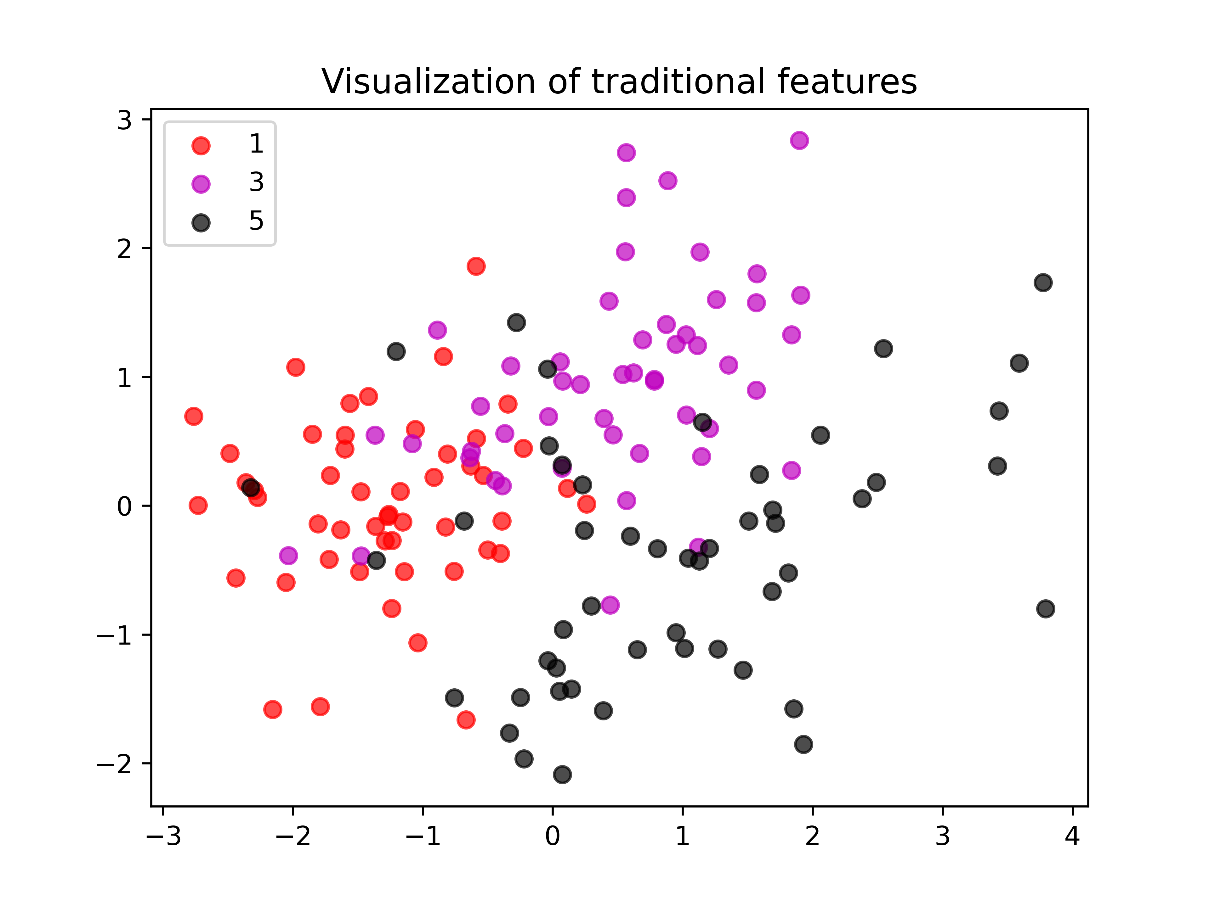
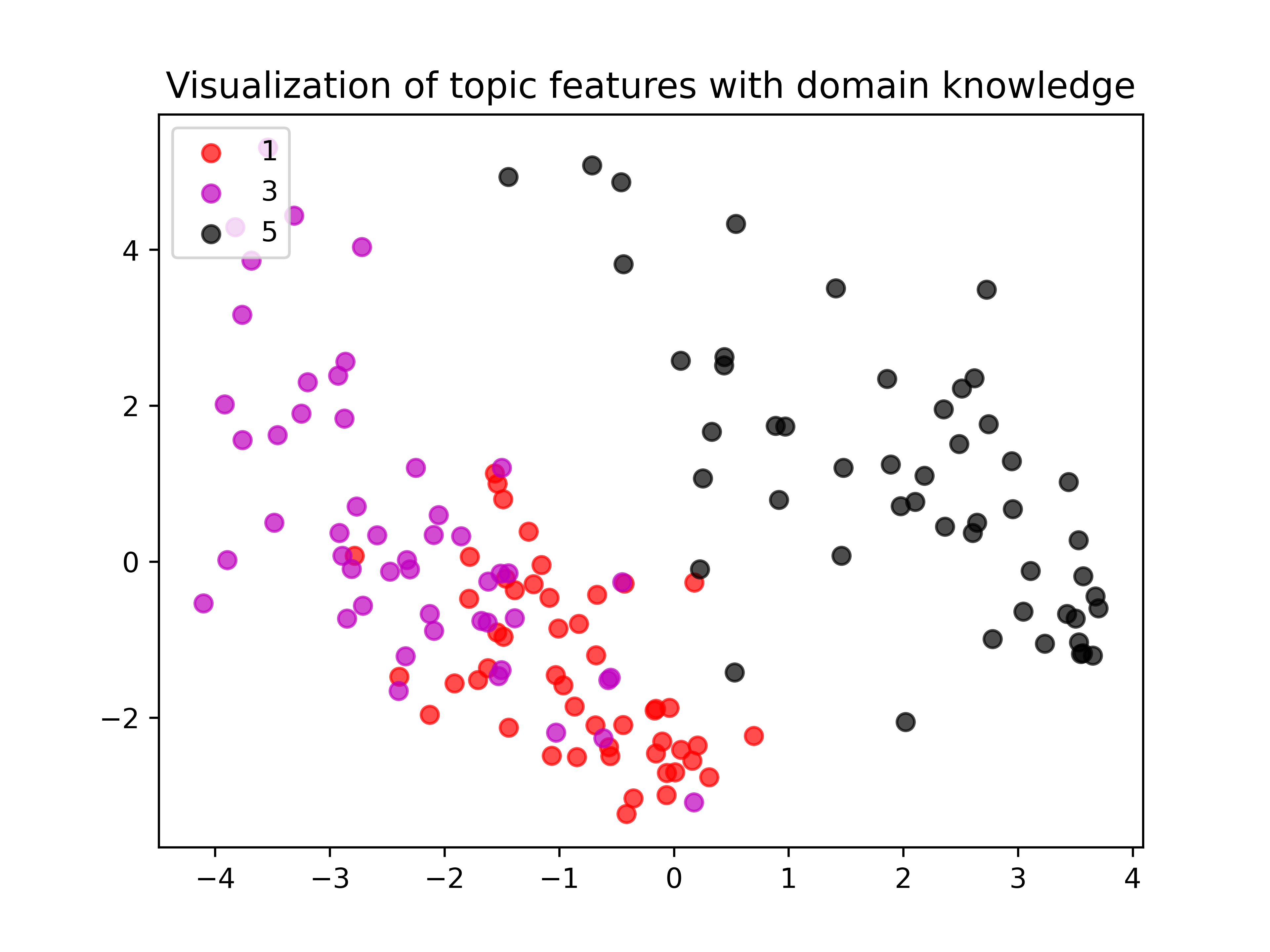
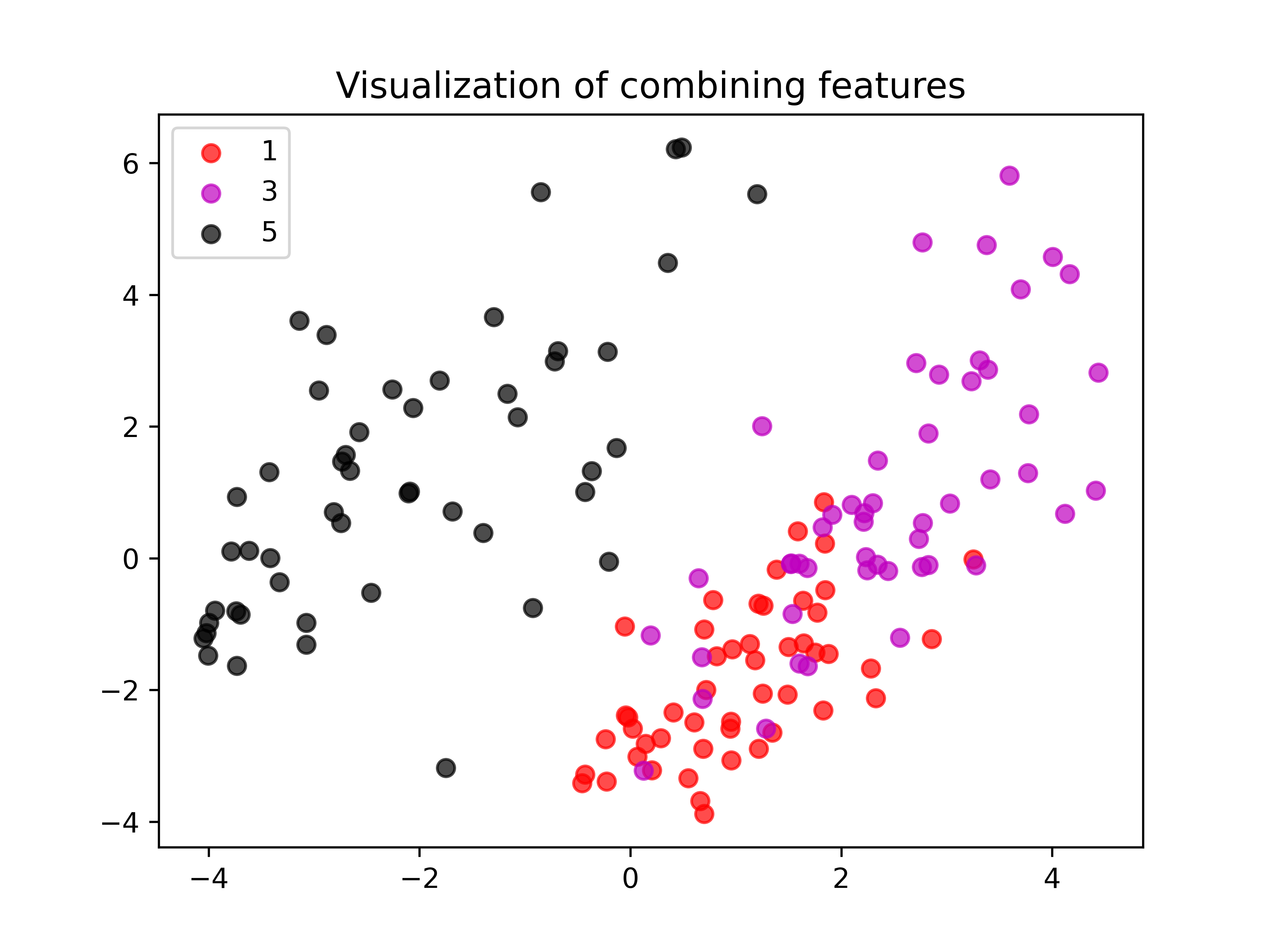
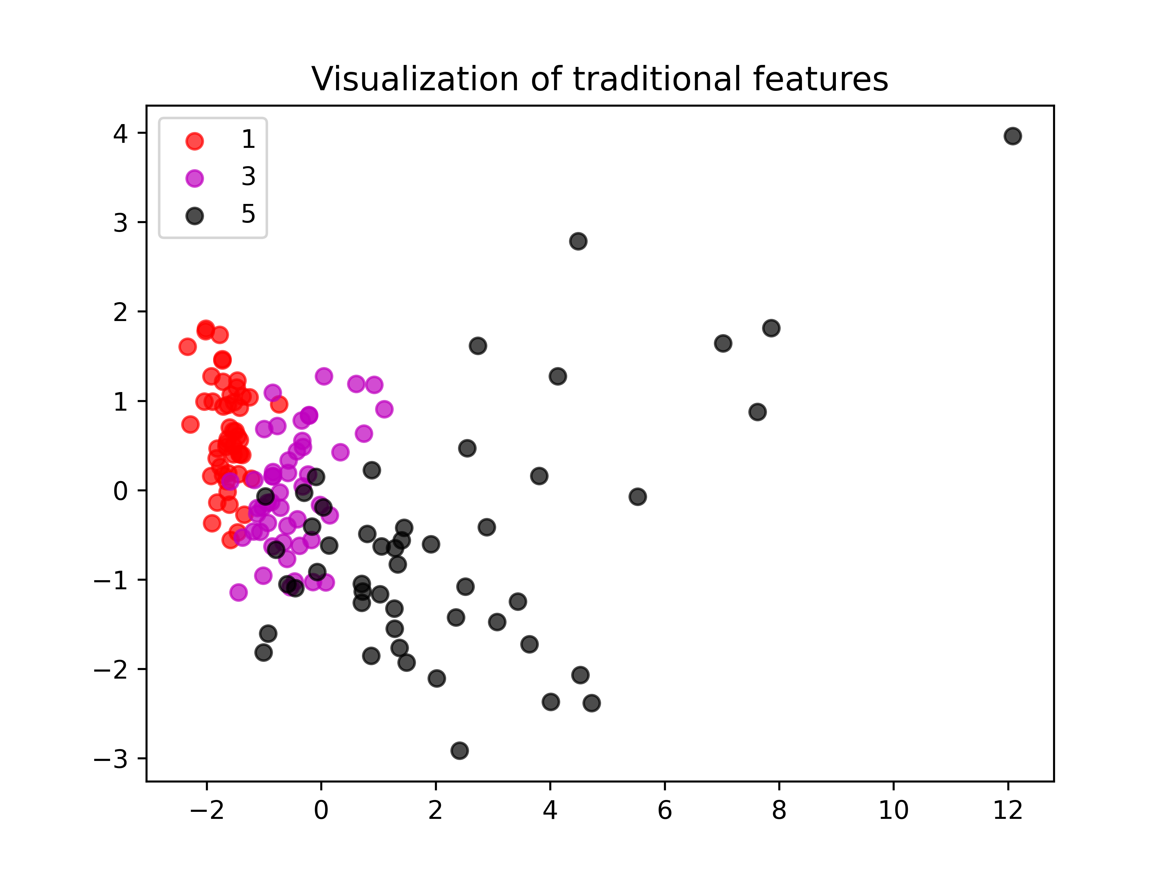
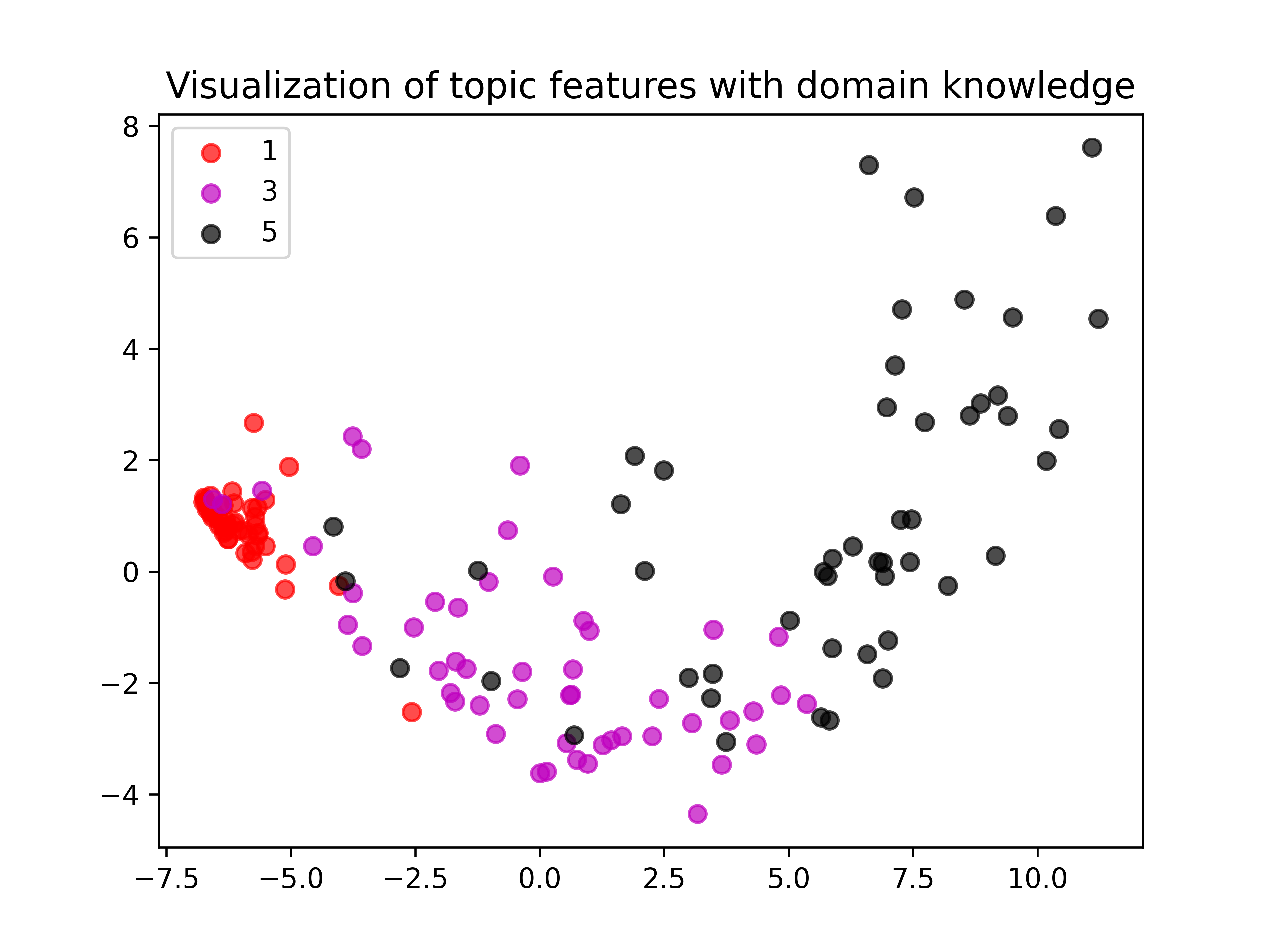
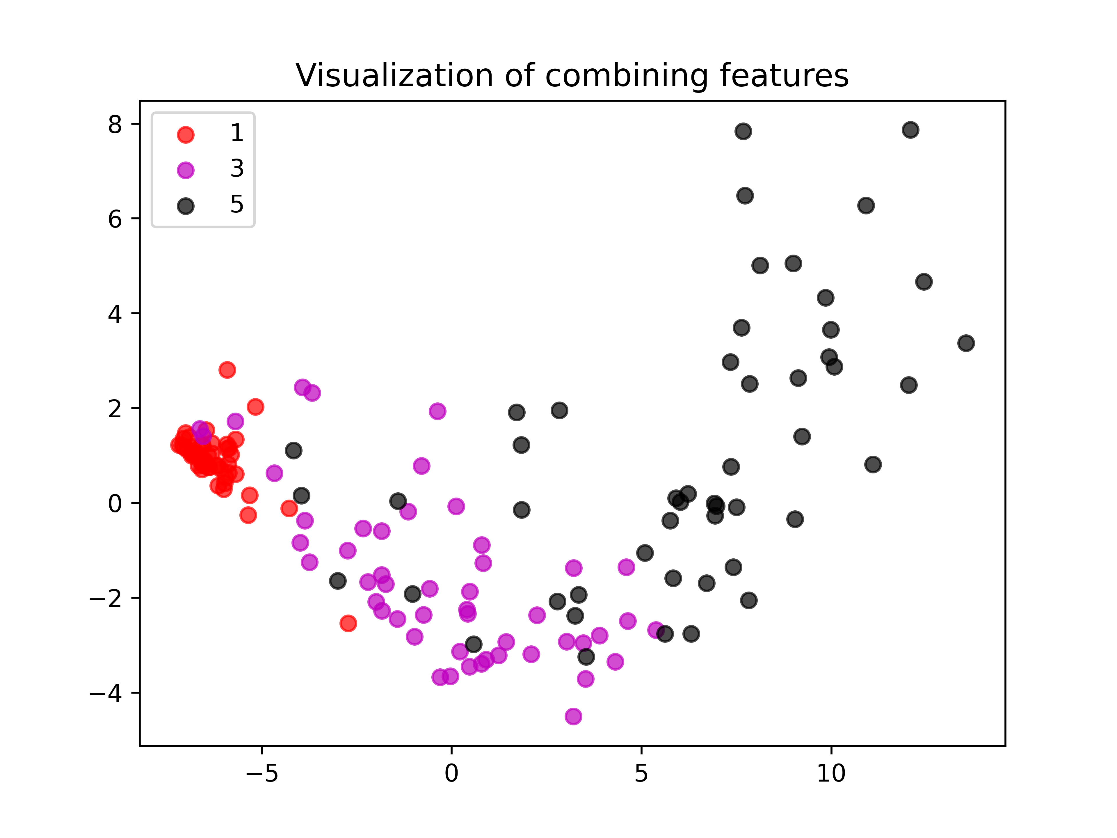
To further explore the impact of topic features with domain knowledge, we visualize the traditional features , difficulty-aware topic features and combining features . Specifically, On WeeBit and ChineseLR, we randomly selected 50 samples from each level of 1, 3 and 5 for visualization, as shown in Figure 3 and 4.
For texts of completely different difficulty, their traditional features are near in the latent space. This shows that traditional features pay more attention to semantic information rather than reading difficulty. By adding difficulty-aware topic features, texts of different difficulty are better differentiated. Further, the combination of two kinds of features achieves a better ability to distinguish reading difficulty.
5.5 Consistency Test with Human Experts
To judge the difficulty level of a text is also a hard task for humans, and so we conduct experiments to investigate how consistent the model’s inference results are with human experts. We collected 200 texts from extracurricular reading materials, and hired three elementary school teachers to do double-blind labeling. Each text is required to annotate with an unique label 1/2/3, corresponding to the first/second/third level.
Our model (denoted as M4) is regarded as a single expert that is equal to the other three human experts (E1/E2/E3). We calculate the Spearman correlation coefficient of annotation results between each pair, and report the results in Table 5.
| Rater | E1 | E2 | E3 | M4 |
| E1 | 1.000 | - | - | - |
| E2 | 1.000 | - | - | |
| E3 | 1.000 | - | ||
| M4 | 1.000 |
On the whole, there is a significant correlation at the 0.01 level between human experts (E1, E2 or E3) and our model. On the one hand, there is still a certain gap between the model and human experts (E1 and E2). On the other hand, the inference results of our model are comparable with the human expert E3. Especially, when E1 is adopted as the reference standard, the consistency of our model prediction is slightly higher than that of E3 (0.836 vs. 0.829). When E2 is regarded as the reference standard, the consistency of our model prediction is slightly lower than that of E3.
Although there is no unified standard for the definition of "text difficulty", which relies heavily on the subject experiences of experts, our model achieves competitive results with human experts.
6 Conclusions
In this paper, we propose a unified neural network model BERT-FP-LBL for readability assessment. We extract difficulty-aware topic features through the Anchored Correlation Explanation method, and fuse linguistic features with BERT representations via projection filtering. We propose a length-balanced loss to cope with the imbalance length distribution. We conduct extensive experiments and detailed analyses on both English and Chinese datasets. The results show that our method achieves state-of-the-art results on three datasets and near-perfect accuracy of 99% on one English dataset.
Limitations
From the perspective of experimental setup, there is no uniform standard for data division and experimental parameter configuration due to less research on readability assessment. This leads to large differences in the results of different studies Qiu et al. (2021); Martinc et al. (2021); Lee et al. (2021), and the results of the corresponding experiments are not comparable. Therefore, objectively speaking, our comparison object is only the baseline model, which lacks a fair comparison with previous work.
From the perspective of readability assessment task, since different datasets have different difficulty scales and different length distributions. In order to ensure the performance on the dataset as much as possible, our length-balanced loss parameters are mainly calculated according to the length distribution of the corresponding dataset, and it is impossible to transfer across datasets directly, which is also a major difficulty in this field. In cross-dataset and cross-language scenarios, there is a lack of a unified approach. Without new ways to deal with the difficulty scales of different datasets, or without large public datasets, developing a general readability assessment model will always be challenging.
Acknowledgement
This work is supported by the National Natural Science Foundation of China (62076008), the Key Project of Natural Science Foundation of China (61936012) and the National Hi-Tech RD Program of China (No.2020AAA0106600).
References
- Azpiazu and Pera (2019) Ion Madrazo Azpiazu and Maria Soledad Pera. 2019. Multiattentive recurrent neural network architecture for multilingual readability assessment. Transactions of the Association for Computational Linguistics, 7:421–436.
- Dale and Chall (1948) Edgar Dale and Jeanne S Chall. 1948. A formula for predicting readability: Instructions. Educational research bulletin, pages 37–54.
- Deutsch et al. (2020) Tovly Deutsch, Masoud Jasbi, and Stuart Shieber. 2020. Linguistic features for readability assessment. arXiv preprint arXiv:2006.00377.
- Devlin et al. (2018) Jacob Devlin, Ming-Wei Chang, Kenton Lee, and Kristina Toutanova. 2018. Bert: Pre-training of deep bidirectional transformers for language understanding. arXiv preprint arXiv:1810.04805.
- Flesch (1948) Rudolph Flesch. 1948. A new readability yardstick. Journal of applied psychology, 32(3):221.
- Gallagher et al. (2017) Ryan J Gallagher, Kyle Reing, David Kale, and Greg Ver Steeg. 2017. Anchored correlation explanation: Topic modeling with minimal domain knowledge. Transactions of the Association for Computational Linguistics, 5:529–542.
- Hansen et al. (2021) Hieronymus Hansen, Adam Widera, Johannes Ponge, and Bernd Hellingrath. 2021. Machine learning for readability assessment and text simplification in crisis communication: A systematic review. In Proceedings of the 54th Hawaii International Conference on System Sciences, page 2265.
- Jiang et al. (2018) Zhiwei Jiang, Qing Gu, Yafeng Yin, and Daoxu Chen. 2018. Enriching word embeddings with domain knowledge for readability assessment. In Proceedings of the 27th International Conference on Computational Linguistics, pages 366–378.
- Lee et al. (2021) Bruce W Lee, Yoo Sung Jang, and Jason Hyung-Jong Lee. 2021. Pushing on text readability assessment: A transformer meets handcrafted linguistic features. arXiv preprint arXiv:2109.12258.
- Lee and Vajjala (2022) Justin Lee and Sowmya Vajjala. 2022. A neural pairwise ranking model for readability assessment. arXiv preprint arXiv:2203.07450.
- Lu et al. (2019) Dawei Lu, Xinying Qiu, and Yi Cai. 2019. Sentence-level readability assessment for l2 chinese learning. In Workshop on Chinese Lexical Semantics, pages 381–392. Springer.
- Maddela and Xu (2018) Mounica Maddela and Wei Xu. 2018. A word-complexity lexicon and a neural readability ranking model for lexical simplification. arXiv preprint arXiv:1810.05754.
- Martinc et al. (2021) Matej Martinc, Senja Pollak, and Marko Robnik-Šikonja. 2021. Supervised and unsupervised neural approaches to text readability. Computational Linguistics, 47(1):141–179.
- Mc Laughlin (1969) G Harry Mc Laughlin. 1969. Smog grading-a new readability formula. Journal of reading, 12(8):639–646.
- Meng et al. (2020) Changping Meng, Muhao Chen, Jie Mao, and Jennifer Neville. 2020. Readnet: A hierarchical transformer framework for web article readability analysis. In European Conference on Information Retrieval, pages 33–49. Springer.
- Paszke et al. (2019) Adam Paszke, Sam Gross, Francisco Massa, Adam Lerer, James Bradbury, Gregory Chanan, Trevor Killeen, Zeming Lin, Natalia Gimelshein, Luca Antiga, et al. 2019. Pytorch: An imperative style, high-performance deep learning library. Advances in neural information processing systems, 32.
- Pennington et al. (2014) Jeffrey Pennington, Richard Socher, and Christopher D Manning. 2014. Glove: Global vectors for word representation. In Proceedings of the 2014 conference on empirical methods in natural language processing (EMNLP), pages 1532–1543.
- Pera and Ng (2014) Maria Soledad Pera and Yiu-Kai Ng. 2014. Automating readers’ advisory to make book recommendations for k-12 readers. In Proceedings of the 8th ACM Conference on Recommender Systems, pages 9–16.
- Perni et al. (2019) Subha Perni, Michael K Rooney, David P Horowitz, Daniel W Golden, Anne R McCall, Andrew J Einstein, and Reshma Jagsi. 2019. Assessment of use, specificity, and readability of written clinical informed consent forms for patients with cancer undergoing radiotherapy. JAMA oncology, 5(8):e190260–e190260.
- Petersen and Ostendorf (2009) Sarah E Petersen and Mari Ostendorf. 2009. A machine learning approach to reading level assessment. Computer speech & language, 23(1):89–106.
- Qin et al. (2020) Qi Qin, Wenpeng Hu, and Bing Liu. 2020. Feature projection for improved text classification. In Proceedings of the 58th Annual Meeting of the Association for Computational Linguistics, pages 8161–8171.
- Qiu et al. (2021) Xinying Qiu, Yuan Chen, Hanwu Chen, Jian-Yun Nie, Yuming Shen, and Dawei Lu. 2021. Learning syntactic dense embedding with correlation graph for automatic readability assessment. arXiv preprint arXiv:2107.04268.
- Qiu et al. (2017) Xinying Qiu, Kebin Deng, Likun Qiu, and Xin Wang. 2017. Exploring the impact of linguistic features for chinese readability assessment. In National CCF Conference on Natural Language Processing and Chinese Computing, pages 771–783. Springer.
- Sare et al. (2020) Antony Sare, Aesha Patel, Pankti Kothari, Abhishek Kumar, Nitin Patel, and Pratik A Shukla. 2020. Readability assessment of internet-based patient education materials related to treatment options for benign prostatic hyperplasia. Academic Radiology, 27(11):1549–1554.
- Schwarm and Ostendorf (2005) Sarah E Schwarm and Mari Ostendorf. 2005. Reading level assessment using support vector machines and statistical language models. In Proceedings of the 43rd annual meeting of the Association for Computational Linguistics (ACL’05), pages 523–530.
- Sheehan et al. (2010) Kathleen M Sheehan, Irene Kostin, Yoko Futagi, and Michael Flor. 2010. Generating automated text complexity classifications that are aligned with targeted text complexity standards. ETS Research Report Series, 2010(2):i–44.
- Song et al. (2018) Yan Song, Shuming Shi, Jing Li, and Haisong Zhang. 2018. Directional skip-gram: Explicitly distinguishing left and right context for word embeddings. In Proceedings of the 2018 Conference of the North American Chapter of the Association for Computational Linguistics: Human Language Technologies, Volume 2 (Short Papers), pages 175–180.
- Su (2019) Xinchun Su. 2019. Compulsory education common vocabulary (draft).
- Tishby et al. (2000) Naftali Tishby, Fernando C Pereira, and William Bialek. 2000. The information bottleneck method. arXiv preprint physics/0004057.
- Vajjala and Lučić (2018) Sowmya Vajjala and Ivana Lučić. 2018. Onestopenglish corpus: A new corpus for automatic readability assessment and text simplification. In Proceedings of the thirteenth workshop on innovative use of NLP for building educational applications, pages 297–304.
- Vajjala and Meurers (2012) Sowmya Vajjala and Detmar Meurers. 2012. On improving the accuracy of readability classification using insights from second language acquisition. In Proceedings of the seventh workshop on building educational applications using NLP, pages 163–173.
- Xia et al. (2019) Menglin Xia, Ekaterina Kochmar, and Ted Briscoe. 2019. Text readability assessment for second language learners. arXiv preprint arXiv:1906.07580.
- Yu et al. (2014) Dingjun Yu, Hanli Wang, Peiqiu Chen, and Zhihua Wei. 2014. Mixed pooling for convolutional neural networks. In International conference on rough sets and knowledge technology, pages 364–375. Springer.
Appendix A Chinese Traditional Features
| Idx | Dim | Feature description |
|---|---|---|
| 1 | 1 | Total number of characters |
| 2 | 1 | Number of character types |
| 3 | 1 | Type Token Ratio (TTR) |
| 4 | 1 | Average number of strokes |
| 5 | 1 | Weighted average number of strokes |
| 6 | 25 | Number of characters with different strokes |
| 7 | 25 | Proportion of characters with different strokes |
| 8 | 1 | Average character frequency |
| 9 | 1 | Weighted average character frequency |
| 10 | 1 | Number of single characters |
| 11 | 1 | Proportion of single characters |
| 12 | 1 | Number of common characters |
| 13 | 1 | Proportion of common characters |
| 14 | 1 | Number of unregistered characters |
| 15 | 1 | Proportion of unregistered characters |
| 16 | 1 | Number of first-level characters |
| 17 | 1 | Proportion of first-level characters |
| 18 | 1 | Number of second-level characters |
| 19 | 1 | Proportion of second-level characters |
| 20 | 1 | Number of third-level characters |
| 21 | 1 | Proportion of third-level characters |
| 22 | 1 | Number of fourth-level characters |
| 23 | 1 | Proportion of fourth-level characters |
| 24 | 1 | Average character level |
| Idx | Dim | Feature description |
|---|---|---|
| 1 | 1 | Total number of words |
| 2 | 1 | Number of word types |
| 3 | 1 | Type Token Ratio (TTR) |
| 4 | 1 | Average word length |
| 5 | 1 | Weighted average word length |
| 6 | 1 | Average word frequency |
| 7 | 1 | Weighted average word frequency |
| 8 | 1 | Number of single-character words |
| 9 | 1 | Proportion of single-character words |
| 10 | 1 | Number of two-character words |
| 11 | 1 | Proportion of two-character words |
| 12 | 1 | Number of three-character words |
| 13 | 1 | Proportion of three-character words |
| 14 | 1 | Number of four-character words |
| 15 | 1 | Proportion of four-character words |
| 16 | 1 | Number of multi-character words |
| 17 | 1 | Proportion of multi-character words |
| 18 | 1 | Number of idioms |
| 19 | 1 | Number of single words |
| 20 | 1 | Proportion of single words |
| 21 | 1 | Number of unregistered words |
| 22 | 1 | Proportion of unregistered words |
| 23 | 1 | Number of first-level words |
| 24 | 1 | Proportion of first-level words |
| 25 | 1 | Number of second-level words |
| 26 | 1 | Proportion of second-level words |
| 27 | 1 | Number of third-level words |
| 28 | 1 | Proportion of third-level words |
| 29 | 1 | Number of fourth-level words |
| 30 | 1 | Proportion of fourth-level words |
| 31 | 1 | Average word level |
| 32 | 57 | Number of words with different POS |
| 33 | 57 | Proportion of words with different POS |
| Idx | Dim | Feature description |
|---|---|---|
| 1 | 1 | Total number of sentences |
| 2 | 1 | Average characters in a sentence |
| 3 | 1 | Average words in a sentence |
| 4 | 1 | Maximum characters in a sentence |
| 5 | 1 | Maximum words in a sentence |
| 6 | 1 | Number of clauses |
| 7 | 1 | Average characters in a clause |
| 8 | 1 | Average words in a clause |
| 9 | 1 | Maximum characters in a clause |
| 10 | 1 | Maximum words in a clause |
| 11 | 30 | Sentence length distribution |
| 12 | 1 | Average syntax tree height |
| 13 | 1 | Maximum syntax tree height |
| 14 | 1 | Syntax tree height <= 5 ratio |
| 15 | 1 | Syntax tree height <= 10 ratio |
| 16 | 1 | Syntax tree height <= 15 ratio |
| 17 | 1 | Syntax tree height >= 16 ratio |
| 18 | 14 | Dependency distribution |
| Idx | Dim | Feature description |
|---|---|---|
| 1 | 1 | Total number of paragraphs |
| 2 | 1 | Average characters in a paragraph |
| 3 | 1 | Average words in a paragraph |
| 4 | 1 | Maximum characters in a paragraph |
| 5 | 1 | Maximum words in a paragraph |
Appendix B Semi-supervised Topic Model Related Parameters
| Pre-training | English | Chinese |
|---|---|---|
| Length range | 3001000 | 5005000 |
| Items | 209018 | 180977 |
| Topics | 120 | 160 |
| Anchor topics | 60 | 80 |
| Anchor strength | 4 | 5 |
| First-level word anchor topics | 16 | 15 |
| Second-level word anchor topics | 21 | 36 |
| Third-level word anchor topics | 14 | 18 |
| Fourth-level word anchor topics | 9 | 11 |
Appendix C SVM model Related Hyperparameters
| Dataset | c | g |
|---|---|---|
| WeeBit | 32 | 0.004 |
| OneStopE | 8 | 0.002 |
| Cambridge | 16 | 0.004 |
| ChineseLR | 64 | 0.032 |
The search range of parameter is [2, 4, 8, 16, 32, 64, 128, 256, 512, 1024, 2048, 4096, 8192, 16384, 32768], and the search range of parameter is [0.002, 0.004, 0.008, 0.016, 0.032, 0.064, 0.128, 0.256, 0.512, 1.024, 2.048, 4.096].