Synthesizing Reactive Test Environments for Autonomous Systems: Testing Reach-Avoid Specifications with Multi-Commodity Flows

Abstract

We study automated test generation for verifying discrete decision-making modules in autonomous systems. We utilize linear temporal logic to encode the requirements on the system under test in the system specification and the behavior that we want to observe during the test is given as the test specification which is unknown to the system. First, we use the specifications and their corresponding non-deterministic Büchi automata to generate the specification product automaton. Second, a virtual product graph representing the high-level interaction between the system and the test environment is constructed modeling the product automaton encoding the system, the test environment, and specifications. The main result of this paper is an optimization problem, framed as a multi-commodity network flow problem, that solves for constraints on the virtual product graph which can then be projected to the test environment. Therefore, the result of the optimization problem is reactive test synthesis that ensures that the system meets the test specifications along with satisfying the system specifications. This framework is illustrated in simulation on grid world examples, and demonstrated on hardware with the Unitree A1 quadruped, wherein dynamic locomotion behaviors are verified in the context of reactive test environments.

I Introduction

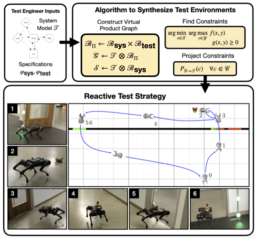
Figure 1: Overview of the test environment synthesis framework and the hardware demonstration.

Operational testing of autonomous systems at various levels of abstraction— from low-level continuous dynamics to high-level discrete decision-making— is essential for verification and validation. In formal methods, testing refers to simulation-based falsification, where inputs to a model of the system are found which result in system violating its requirements [1, 2, 3, 4, 5, 6, 7]. Falsification methods typically minimize a robustness metric associated with the formal specifications of the system to find inputs that result in falsifying traces [8, 9, 10]. However, another approach to testing is to have test engineers hand-design test scenarios as seen in the qualification tests of the DARPA Urban Challenge [11, 12]. In this work, we bridge these two approaches by leveraging test engineer expertise at the specification level and then automating the construction of the test environment for testing discrete, long-horizon decision-making in robotic systems. In the last decade, the control synthesis community has demonstrated the effectiveness of using temporal logic to specify formal requirements for robotic systems [13, 14, 15, 16]. Furthermore, we assume that via the use of rulebooks and industry standard manuals [17, 18, 19], a test engineer can provide these high-level descriptions on the desired test outcomes using temporal logic.

Our notion of testing in this work is also complementary to falsification — we seek to construct a test environment to observe a desired high-level behavior, on which falsification can then be applied to determine the worst-case scenario which can provide confidence that the system will behave correctly in operational environments. Furthermore, falsification algorithms oftentimes search over continuous inputs to find a failure case [20, 21, 22, 23]. We envision that falsification could be used to refine the test environments generated by our approach.

Our approach to test generation shares similarities with existing methods, but has key differences. Similar to [24], we characterize the mission requirements on the system as a system specification, and characterize the desired behavior observed during the test via a test specification, which is unknown to the system. However, unlike [24], we seek to construct the test environment, by constraining actions that the system can take, such that: a) the system can still satisfy its requirements, and b) the test specification is satisfied in a successful test execution (1). Additionally, we seek to synthesize tests in which the system is not too restricted in its decision-making (2).

Building upon the results of [25], the key contributions of this paper are (i) framing the problem of synthesizing test environments for reach-avoid specifications in linear temporal logic (LTL) as a multi-commodity network flow problem, (ii) presenting an efficiently solvable convex-concave min-max optimization-based relaxation that results in a constrained test, (iii) demonstrating the approach by executing the resulting test strategy to reactively test dynamic locomotion behaviors of the Unitree A1 quadruped. A key advantage of our method is that the synthesized test is reactive — the constraints visible to the system under test are reactive to the system state and depend on the system’s strategy, which is not known to the tester a priori.

II Background

II-A Temporal Logic, Transition Systems, and Automata

Linear temporal logic (LTL) can describe temporal properties on a trace of propositional formulas [26]. The syntax of LTL is comprised of both logical ($\wedge$ and, $\vee$ or, and $\neg$ negation) and temporal operators ($\bigcirc$ next, $\square$ always, $\lozenge$ eventually, and $\mathcal{U}$ until) operators. LTL can specify requirements on high-level decision-making in autonomous systems such as safety $\square(\varphi^{s}_{\text{sys}})$, progress $\lozenge(\varphi^{p}_{\text{sys}})$, and fairness $\square\lozenge(\varphi^{f}_{\text{sys}})$.

A nondeterministic Büchi automaton (NBA) [27] is a tuple $\mathcal{B}=(Q,2^{AP},\delta,Q_{0},F)$, where $Q$ represents the states, $AP$ is the set of atomic propositions, $\delta$ represents the transition function, $Q_{0}\subseteq Q$ represents the initial states, and $F\subseteq Q$ is the set of acceptance states. A transition system is a tuple $\mathcal{T}=(S,A,E,I,AP,L)$ where $S$ is a set of states, $A$ is the set of actions, $E:S\times A\rightarrow S$ is the transition relation, $I\subseteq S$ is the set of initial states, $AP$ is the set of atomic propositions, and $L:S\rightarrow 2^{AP}$ is a labeling function that indicates the set of atomic propositions that evaluate to true at a particular state.

Definition 1 (Product Automaton).

A product automaton is the synchronous product of a transition system $\mathcal{T}=(S,A,E,I,AP,L)$ and a NBA $\mathcal{B}=(Q,2^{AP},\delta,Q_{0},F)$, is the tuple $\mathcal{T}\otimes\mathcal{B}=(S^{\prime},A,E^{\prime},I^{\prime},AP^{\prime},L^{\prime})$, where:

• $S^{\prime}=S\times Q$,

• $\forall s,t\in S$, $\forall q,p\in Q$ such that $s\overset{a}{\rightarrow}t$ and $\delta(q,L(t))=p$, then, $(s,q)\overset{a}{\rightarrow}^{\prime}(t,p)$,

• $I^{\prime}=\{(s_{0},q):s_{0}\in I,\,\exists q_{0}\in Q_{0}\text{ s.t. }q_{0}\overset{L(s_{0})}{\rightarrow}q\}$,

• $AP^{\prime}=Q$, and

• $L^{\prime}:S\times Q\rightarrow 2^{Q}$ such that $L^{\prime}((s,q))=\{q\}$.

Definition 2 (Asynchronous Product Automaton).

An asynchronous product automaton of finite state automata $\mathcal{A}_{1},\ldots,\mathcal{A}_{n}$ is the finite state automaton $\mathcal{A}_{\Pi}=(S_{\Pi},s_{0,\Pi},L_{\Pi},F_{\Pi},T_{\Pi})$, where:

• $S_{\Pi}:=S_{1}\times\ldots\times S_{n}$, the Cartesian product of the states of the individual product automata,

• $s_{0,\Pi}=(s_{01},\ldots,s_{0n})$, the $n-$tuple representing initial conditions,

• $L_{\Pi}:=L_{1}\cup\ldots\cup L_{n}$, where $L_{i}=2^{AP_{i}}$ for all $i\in\{1,\ldots,n\}$,

• $T_{\Pi}:=((u_{1},\ldots,u_{n}),l,(v_{1},\ldots,v_{n}))$ such that $\exists i$ and $1\leq i\leq n$, $(u_{i},l,v_{i})\in T_{i}$ and $\forall j\neq i$, $u_{j}=v_{j}$,

• $F_{\Pi}:=(s_{1},\ldots,s_{n})\in S$ such that $\exists i$ such that $s_{i}\in F_{i}$.

II-B System and Test Environment

We utilize the notion of a system specification and a test specification, which represent requirements on the system under test and the test environment, respectively [24]. The system specification is assumed to be given, while the system does not necessarily have knowledge of the entire test specification. In this work we will frame the system specification and the test specification as reach-avoid type specifications defined as

$$\varphi_{\text{sys}}=\square\varphi^{s}_{\text{sys}}\land\lozenge\varphi^{p}_{\text{sys}},\>\varphi_{\text{test}}=\square(\varphi^{s}_{\text{test}})\land\bigwedge_{i}\lozenge(\varphi^{p}_{\text{test}})_{i},$$ (1)

which capture the safety and progress requirements on the system, and the tester respectively. We show that it is possible to model the set of feasible test executions using network flows on an automaton.

Definition 3 (Network Flow).

A network flow is a tuple $\mathcal{N}=\langle V,E,c,s,t\rangle$ where $V$ is a set of vertices, $E$ is a set of directed edges, $E\subseteq V\times V$, $c$ is a capacity function for the amount of flow that each edge can transfer, and $s\in V$ are the source vertices and $t\in V$ are the target sink vertices. In a single network flow, each edge is associated with a single flow, while in a multi-commodity setting, multiple flows are associated with each edge. An extension of network flows to the game setting is known as a flow game [28]. While our work involves solving a Stackleberg game over a multi-commodity flow network, it differs from [28] in that the tester is not completely adversarial.

III Synthesizing Test Environments

This section sets up the test generation problem statement and introduces a running example to illustrate the approach we take in this paper.

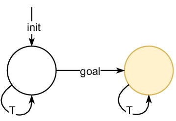
(a) System Büchi automaton $B_{\text{sys}}$.

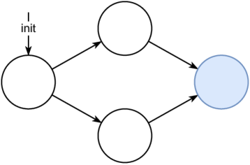
(b) Tester Büchi automaton $\mathcal{B}_{\text{test}}$.

(c) Specification product automaton $\mathcal{B}_{\pi}$.

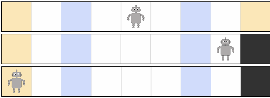
(d) Resulting Test Execution.

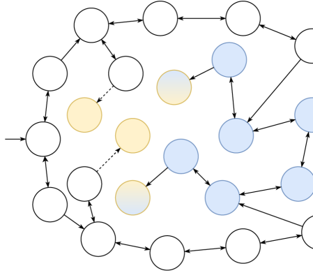
(e) Virtual game graph $\mathcal{G}=\mathcal{T}\otimes\mathcal{B}_{\pi}$. The initial state corresponds to $\mathtt{S}$, (partially) yellow states to $\mathtt{T}$, and exclusively blue states to $\mathtt{I}$.

Figure 2: Büchi automata for the system specification, the test specification and the product automaton $\mathcal{B}_{\pi}=\mathcal{B}_{\text{test}}\times\mathcal{B}_{\text{sys}}$, and the virtual product graph $\mathcal{G}$ for the corridor navigation example. The accepting states of the system are shaded in yellow and the acceptance states of the tester are shaded in blue, with nodes shaded in both yellow and blue representing acceptance states of both tester and system. Transition labels and self-loops have been omitted in $\mathcal{B}_{\text{test}}$, $\mathcal{B}_{\pi}$, and $\mathcal{G}$ for clarity.

III-A Problem Statement

The system and test specifications are written at the same level of abstraction as the model of the system characterized by the transition system $\mathcal{T}$. We require that the sub-formulas of the test specifications, $\varphi^{s}_{\text{test}}$ and $\varphi^{p}_{\text{test}}$ in equation 1, be high-level descriptions of desired test scenarios provided by a test engineer. In this way, the task of describing the behavior of the system to be observed during the test is left to the test engineer, but the process of synthesizing a corresponding test environment can be automated.

Problem 1.

Given a discrete abstraction of a system model $\mathcal{T}=(S,A,E,I,AP,L)$, and system and test specifications, $\varphi_{\text{sys}}$ and $\varphi_{\text{test}}$, defined over the set $AP$, find the set of transitions of the system $E_{\text{cut}}\subset E$ that need to be constrained such that all traces $\sigma\models\varphi_{\text{sys}}$ of the constrained system on $\mathcal{T}=(S,A,E_{\text{cut}},I,AP,L)$ satisfy the following property:

$$\sigma\models\varphi_{\text{sys}}\implies\sigma\models\varphi_{\text{test}}.\vspace{-1mm}$$ (2)

In other words, a trace of the constrained system that satisfies the system specification must also satisfy the test specification, and the constraints are synthesized such that there always exists a trace satisfying the system specification. In addition to determining constraints that result in test executions of the system abiding by equation (2), we do not want the system to be so constrained that it does not have much freedom in decision-making during the test. In this work, we use maximum network flow as a proxy for the maximum freedom a robot has to achieve its specifications, and we present an algorithmic framework that addresses both these problems on examples in both simulation and hardware.

III-B Running Example: Robot in a corridor

Consider a corridor in a grid world shown in figure 2. The system under test is starting in the middle of the corridor with the goal of reaching either end. The dynamics are simple grid world dynamics enabling horizontal transitions to neighboring grid cells. The test behavior that we want to observe is that the system passes through the two blue grid cells $\varphi_{\text{test}}=\lozenge\text{key}_{1}\land\lozenge\text{key}_{2}$. The system specification is given as $\varphi_{\text{sys}}=\lozenge\text{goal}$, which corresponds to the yellow grid cells. We then constrain the system transitions according to our algorithm by placing obstacles on the grid cells, which we will show in the following sections.

III-C Constructing Product Automata

We draw from automata theory to define the specification product automaton and virtual product graph. The product automaton of the system transition $\mathcal{T}$ and the Büchi automaton corresponding to the specification $\varphi_{\text{sys}}$, $\mathcal{T}\otimes\mathcal{B}_{\text{sys}}$, is denoted by the tuple $\mathcal{S}=(S_{\text{sys}},A,E_{\text{sys}},I_{\text{sys}},AP_{\text{sys}},L_{\text{sys}})$. The asynchronous product is used to construct the specification product automaton of the system and test Büchi automata. The product automaton of the transition system, $\mathcal{T}$, and the specification product automaton is denoted as the virtual product graph $\mathcal{G}$. It is for this product automaton $\mathcal{G}$, that we will be synthesizing constraints.

Definition 4 (Specification Product Automaton).

The specification product automaton $\mathcal{B}_{\Pi}=\mathcal{B}_{\text{sys}}\times\mathcal{B}_{\text{test}}$ is the asynchronous product of the Büchi automata of the system and the test specification. In particular, $\mathcal{B}_{\Pi}.F=\{(q_{\text{sys}},q_{\text{test}})\in\mathcal{B}_{\Pi}.Q|q_{\text{sys}}\in\mathcal{B}_{\text{sys}}.F\}\cup\{(q_{\text{sys}},q_{\text{test}})\in\mathcal{B}_{\Pi}.Q|q_{\text{test}}\in\mathcal{B}_{\text{test}}.F\}$.

Definition 5 (Virtual Product Graph).

The synchronous product automaton of system transition $\mathcal{T}$ and the NBA $\mathcal{B}_{\Pi}$ is the virtual product graph $\mathcal{G}=\mathcal{T}\otimes\mathcal{B}_{\Pi}$. In tuple form, we denote $\mathcal{G}=(S^{\prime},A,E^{\prime},I^{\prime},AP^{\prime},L^{\prime})$.

Definition 6 (Source, Intermediate and Target Nodes).

The source ($\mathtt{S}$), intermediate ($\mathtt{I}$) and target ($\mathtt{T}$) are the set of nodes on the virtual product graph $\mathcal{G}$ with the following properties:

$$\mathtt{S}=\{(s_{0},q_{0})\in S^{\prime}|q_{0}\in\mathcal{B}_{\Pi}.Q\}$$ (3)

$$\mathtt{I}=\{(s,(q_{\text{sys}},q_{\text{test}}))\in S^{\prime}|q_{\text{test}}\in\mathcal{B}_{\text{test}}.F,\,q_{\text{sys}}\notin\mathcal{B}_{\text{sys}}.F\}$$

$$\mathtt{T}=\{(s,(q_{\text{sys}},q_{\text{test}}))\in S^{\prime}|q_{\text{sys}}\in\mathcal{B}_{\text{sys}}.F\}$$

The source nodes $\mathtt{S}$ represent the initial conditions of the test, the intermediate nodes $\mathtt{I}$ represent the acceptance states corresponding to the test specification, and the target nodes $\mathtt{T}$ represent the acceptance states corresponding to the system specification. For the running example, the automata corresponding to $\mathcal{B}_{\text{sys}}$, $\mathcal{B}_{\text{test}}$, $\mathcal{B}_{\Pi}$ are illustrated in Figure 2-2. the virtual product graph $\mathcal{G}$ and the corresponding source, intermediate and target nodes are illustrated in Figure 2.

Problem 2.

Given the setting in Problem 1, synthesize the set of edge constraints $E^{\prime}_{\text{cut}}$ on the virtual product graph $\mathcal{G}$ such that flows from $\mathtt{S}$ to $\mathtt{T}$ is maximized, and all possible traces on $\mathcal{G}$ from $\mathtt{S}$ to $\mathtt{T}$ comprise of a node in $\mathtt{I}$.

III-D Multi-Commodity Flows and Bilevel Optimization

To synthesize constraints $E^{\prime}_{\text{cut}}$ on the virtual product graph $\mathcal{G}$, we use multi-commodity flows on $\mathcal{G}$ and present a bilevel optimization to find cuts. These constraints are such that a) there exists a system controller that can satisfy the system specification ($\sigma\models\varphi_{\text{sys}}$), and that for every satisfying trace, the test specification is also satisfied (equation (2)), and b) the set of cuts $E^{\prime}_{\text{cut}}$ on $\mathcal{G}$ result in maximum flow from $\mathtt{S}$ to $\mathtt{T}$. We then map these synthesized constraints $E^{\prime}_{\text{cut}}$ to constraints $E_{\text{cut}}$ on system transitions $\mathcal{T}$.

Given a graph $\mathcal{G}$ with $\mathtt{S}$, $\mathtt{I}$, and $\mathtt{T}$, a brute force approach to solving Problems 1 and 2 is not viable, as it would involve a) finding a set of paths $P_{\mathtt{S}\rightarrow\mathtt{I}}$ realizing max-flow from $\mathtt{S}$ to $\mathtt{I}$, and b) finding a set of paths $P_{\mathtt{I}\rightarrow\mathtt{T}}$ realizing max flow from the $\mathtt{I}$ to $\mathtt{T}$, such that $P_{\mathtt{S}\rightarrow\mathtt{I}}$ and $P_{\mathtt{I}\rightarrow\mathtt{T}}$ are disjoint except for the intermediate $\mathtt{I}$. Finding such a feasible pair of $P_{\mathtt{S}\rightarrow\mathtt{I}}$ and $P_{\mathtt{I}\rightarrow\mathtt{T}}$ would take exponential time because enumerating all paths is exponential in the size of the graph [29].

To address this combinatorial problem, we formulate a bilevel optimization that relaxes edge cuts to take fractional values. These relaxed constraints, in addition to our choice of the objective function, makes the optimization tractable. While the cut values of some edges take on fractional values due to the relaxation, we find empirically that these fractional cuts are not relevant to constraining the flow. The system and tester are players that optimize for different flows on the same virtual product graph $\mathcal{G}$. The system player maximizes flow $f_{\mathtt{S}\rightarrow\mathtt{T}}$, defined from $\mathtt{S}$ to $\mathtt{T}$, with the flow into and out of the intermediate ($\mathtt{I}$) constrained to zero. These represent behaviors of the system satisfying $\varphi_{\text{sys}}$ without satisfying $\varphi_{\text{test}}$. The tester player: i) maximizes flow $f_{\mathtt{S}\rightarrow\mathtt{I}}$ (defined from $\mathtt{S}$ to $\mathtt{I}$), ii) maximizes flow $f_{\mathtt{I}\rightarrow\mathtt{T}}$ (defined from $\mathtt{I}$ to $\mathtt{T}$), and iii) minimizes flow $f_{\mathtt{S}\rightarrow\mathtt{T}}$ that bypasses the intermediate $\mathtt{I}$. We use the multi-commodity network flows to simultaneously reason about several flows on $\mathcal{G}$ — maximizing flows $f_{\mathtt{S}\rightarrow\mathtt{I}}$ and $f_{\mathtt{I}\rightarrow\mathtt{T}}$, and cutting the flow $f_{\mathtt{S}\rightarrow\mathtt{T}}$. However, unlike the canonical multi-commodity flow framework [30], our flows do not compete for edge capacities. Instead, the flows are coupled by the placement of cuts by constraining flow along the edges. Therefore, the tester does not directly set the flow $f_{\mathtt{S}\rightarrow\mathtt{T}}$, but indirectly constrains it by placing cuts on system transitions. This multi-commodity flow-based bilevel optimization is given in (8). The variables of the optimization are normalized by the total flow $F$ on $\mathcal{G}$, which is defined as follows,

$$F=\min\{\sum_{v:(\mathtt{S},v)\in E^{\prime}}f^{(\mathtt{S},v)}_{\mathtt{S}\rightarrow\mathtt{I}},\sum_{v:(\mathtt{I},v)\in E^{\prime}}f^{(\mathtt{I},v)}_{\mathtt{I}\rightarrow\mathtt{T}}\}.\vspace{-2mm}$$ (4)

We require the auxiliary variable $t:=1/F$ to re-write network flow constraints in the normalized form. For every edge $e\in E^{\prime}$, let $d^{e}$ represent the constraint on the edge — $d^{e}=t$ means that the edge $e$ is cut or fully constrained and $d^{e}=0$ means that the edge $e$ is unconstrained. Similarly, for every $e\in E^{\prime}$, $f^{e}_{S\rightarrow\mathtt{I}}$, $f^{e}_{\mathtt{I}\rightarrow\mathtt{T}}$, and $f^{e}_{\mathtt{S}\rightarrow\mathtt{T}}$ are the respective flow values on edge $e$ in $\mathcal{G}$. As the outer (min) player, the tester variables are the flows $f^{e}_{\mathtt{S}\rightarrow\mathtt{I}}$ and $f^{e}_{\mathtt{I}\rightarrow\mathtt{T}}$, edge cuts $d^{e}$, and the auxiliary variable $t$. The objective function corresponds to the tester synthesizing constraints $d^{e}$ such that total flow $F$ is maximized while max-flow of $f_{\mathtt{S}\rightarrow\mathtt{T}}$ is minimized. Likewise, the system player gets to maximize flow $f_{\mathtt{S}\rightarrow\mathtt{T}}$. Next, the constraints of the bilevel optimization are detailed. Capacity constraints determine the maximum flow allowed on an edge. The capacity constraints for normalized variables in this optimization are given as follows,

$$\forall e\in E^{\prime}, 0\leq d^{e}\leq t, 0\leq f^{e}_{\mathtt{S}\rightarrow\mathtt{I}}\leq t,$$ (c1)

$$0\leq f^{e}_{\mathtt{S}\rightarrow\mathtt{T}}\leq t, 0\leq f^{e}_{\mathtt{I}\rightarrow\mathtt{T}}\leq t.$$

Cut constraints correspond to the cut variable and flow variable of an edge competing for its capacity. For all $k\in\{\mathtt{S}\rightarrow\mathtt{I},\mathtt{I}\rightarrow\mathtt{T},\mathtt{S}\rightarrow\mathtt{T}\}$, the cut constraints are as follows,

$$\forall e\in E^{\prime},\quad d^{e}+f^{e}_{k}\leq t.\vspace{-1mm}$$ (c2)

Flow conservation constraints ensure that the total flow entering entering a node is equal to the total flow leaving the node (unless the node is a source or a target). For $k\in\{\mathtt{S}\rightarrow\mathtt{I},\mathtt{I}\rightarrow\mathtt{T},\mathtt{S}\rightarrow\mathtt{T}\}$, the conservation constraints are as follows,

$$\forall v\in S^{\prime}\sum_{u:(u,v)\in E^{\prime}}f^{(u,v)}_{k}=\sum_{u:(v,u)\in E^{\prime}}f^{(v,u)}_{k}.$$ (c3)

Finally, equation (4) can be re-written as the following constraint after normalizing the variables,

$$1\leq\sum_{v:(\mathtt{S},v)\in E}f^{(\mathtt{S},v)}_{\mathtt{S}\rightarrow\mathtt{I}},\,\quad 1\leq\sum_{v:(\mathtt{I},v)\in E}f^{(\mathtt{I},v)}_{\mathtt{I}\rightarrow\mathtt{T}}.$$ (c4)

Our framework can synthesize test environments by constraining system actions, not by enforcing them. When the bilevel optimization finds constraints on the virtual product $\mathcal{G}$, it takes into account tester behavior unknown to the system in the form of the test specification. The framework guarantees that under the synthesized constraints, there always exists a system trace $\sigma=s^{\prime}_{0}s^{\prime}_{1}\ldots$ on $\mathcal{G}$ satisfying the system specification. However, this could return constraints for which at some temporal instances in the test execution, there is no path for satisfying trace on the system product automaton $S$. During a test execution, these constraints on the system could potentially translate to the system, at that temporal instance, not being able to re-plan to satisfying its requirements. If possible, our framework should return constraints for which at every temporal instance of the test execution, the system should find a feasible path to satisfying its requirements. We add the following constraints to ensure that for the state $\sigma_{t}=s^{\prime}_{t}$ during the test, for which the state of the system corresponds to $s_{t}$, there exists a path to the acceptance states of $\varphi_{\text{sys}}$ on $\mathcal{S}$.

It is not necessary that all of these constraints on the virtual product graph $\mathcal{G}$ be visible at any given system state $s_{t}$. This feature allows for the tester to place constraints reactively to the system state $s_{t}$. To reason about constraints that would be visible to the system at $s_{t}$, we define mappings between the product automata. The first mapping, $M_{B_{\Pi}\rightarrow\mathcal{G}}$, from the specification product automaton $B_{\Pi}$ to $\mathcal{G}$ defines the states of $\mathcal{G}$ that are active for a state $q\in B_{\Pi}.Q$:

$$M_{B_{\Pi}\rightarrow\mathcal{G}}(q)=\{(s,(q_{\text{sys}},q_{\text{test}}))\in S^{\prime}|q=(q_{\text{sys}},q_{\text{test}})\}.$$ (5)

At $s^{\prime}_{t}=(s_{t},q_{t})$ during the test execution, state $q_{t}$ is active in the specification product automaton $B_{\Pi}$. The outgoing edges of nodes in $M_{B_{\Pi}\rightarrow\mathcal{G}}(q_{t})$ represent the set of constraints that can be mapped to $\mathcal{S}$ at $q_{t}$. Let $C_{\mathcal{G}}(q_{t})$ denote these edges:

$$C_{\mathcal{G}}(q_{t})=\{(e,d^{e})|e=(u,v)\in E^{\prime}\text{ s.t. }u\in M_{B_{\Pi}\rightarrow\mathcal{G}}(q_{t})\}.$$ (6)

By construction, every edge-constraint pair $(e,d_{e})$ in $C_{\mathcal{G}}(q_{t})$ maps to an edge-constraint pair in $\mathcal{S}$. Let $V_{\mathcal{G}\rightarrow\mathcal{S}}$ map the nodes from $\mathcal{G}$ to $\mathcal{S}$. If $v=(s,(q_{\text{sys}},q_{\text{test}})\in S^{\prime}$, then $V_{\mathcal{G}\rightarrow\mathcal{S}}(v)=(s,q_{\text{sys}})\in S_{\text{sys}}$. Therefore, for every $e=((u,v),d^{e})\in C_{\mathcal{G}}(q_{t})$, the corresponding edge-constraint pair on $\mathcal{S}$ is $((V_{\mathcal{G}\rightarrow\mathcal{S}}(u),V_{\mathcal{G}\rightarrow\mathcal{S}}(v)),d^{e})$. We denote this map as $M_{\mathcal{G}\rightarrow\mathcal{S}}$, and the mapping is formally stated as follows,

$$M_{\mathcal{G}\rightarrow\mathcal{S}}((u,v),d^{e})=(((V_{\mathcal{G}\rightarrow\mathcal{S}}(u),V_{\mathcal{G}\rightarrow\mathcal{S}}(v)),d^{e}).$$ (7)

Note that the constraint found on $G$ is mapped one-to-one to the constraint on $S$. This node mapping also provides the initial and acceptance states in $S$ that are relevant denoted $V_{\mathcal{G}\rightarrow\mathcal{S}}(\mathtt{S})$ and $V_{\mathcal{G}\rightarrow\mathcal{S}}(\mathtt{T})$, respectively. Thus, the constraints that are active on $\mathcal{S}$ at $q\in\mathcal{B}_{\Pi}.Q$ are as follows,

$$C_{\mathcal{S}}(q_{t})=\{M_{\mathcal{G}\rightarrow\mathcal{S}}(e,d^{e})|(e,d^{e})\in C_{\mathcal{G}}(q)\}.$$ (c5)

Remark 1.

$C_{\mathcal{S}}(q_{t})$ represents the largest set of constraints that could be visible to the system at $s_{t}$. Note that we say largest possible because the constraints visible to the system at $s_{t}$ are the constraints on $\mathcal{S}$ projected onto system transition $\mathcal{T}$ at that instant. However, not all constraints in $C_{\mathcal{S}}(q_{t})$ might apply to the system, which is in state $s_{t}$.

For every edge $e\in E_{\text{sys}}$ and for every $q\in\mathcal{B}_{\Pi}.Q$, let $f^{e}_{\mathcal{S}}(q)$ denote the flow from source $V_{\mathcal{G}\rightarrow\mathcal{S}}(\mathtt{S})$ to target $V_{\mathcal{G}\rightarrow\mathcal{S}}(\mathtt{T})$. For brevity, we do not elaborate the constraints here, but the flow variables $f^{e}_{\mathcal{S}}(q)$ must respect the standard network flow constraints in equations (c1)-(c3). We require the following condition to be satisfied:

$$\forall q\in\mathcal{B}_{\Pi}.Q,\quad\sum_{e=(V_{\mathcal{G}\rightarrow\mathcal{S}}(\mathtt{S}),v)\in E_{\text{sys}}}f^{e}_{\mathcal{S}}(q)\geq 1.$$ (c6)

Since the above constraint is defined from a fixed source $V_{\mathcal{G}\rightarrow\mathcal{S}}(\mathtt{S})$ to target $V_{\mathcal{G}\rightarrow\mathcal{S}}(\mathtt{T})$ on $\mathcal{S}$, we assume that from every state $(s,q_{\text{sys}})\in S_{\text{sys}}$, there exists an edge to the source $V_{\mathcal{G}\rightarrow\mathcal{S}}(\mathtt{S})$. For the examples of this paper with the system specifications of the class (1), this is always the case. In future work, we would like to prove these properties for a larger class of specifications and transition systems. Therefore, the bilevel optimization for synthesizing reactive constraints is as follows,

$$\text{MCF-OPT}(\lambda):$$ (8)

$$\operatorname*{\arg\!\min}_{f^{e}_{\mathtt{S}\rightarrow\mathtt{I}}f^{e}_{\mathtt{I}\rightarrow\mathtt{T}},d^{e},t,f^{e}_{\mathcal{S}}(q)} \operatorname*{\arg\!\max}_{f^{e}_{\mathtt{S}\rightarrow\mathtt{T}}}\quad t+\lambda\sum_{v:(s_{3},v)\in E^{\prime}}f^{e}_{\mathtt{S}\rightarrow\mathtt{T}}$$

s.t. $$\eqref{eq:cap}-\eqref{eq:proj},$$

where the regularization parameter $\lambda$ penalizes the tester (and rewards the system) on $f_{S\rightarrow T}$ flow. This optimization is in the form of a convex-concave min-max Stackleberg game with dependent constraint sets studied in[31], for which there always exists a solution.

Algorithm 1 Constraining Virtual Product Graph $\mathcal{G}$

1:procedure Automata($\mathcal{T},\varphi_{\text{sys}},\varphi_{\text{test}}$)

2:     $\mathcal{B}_{\text{sys}}\leftarrow\text{BA}(\varphi_{\text{sys}})$ $\triangleright$ System Büchi automaton

3:     $\mathcal{B}_{\text{test}}\leftarrow\text{BA}(\varphi_{\text{test}})$ $\triangleright$ Tester Büchi automaton

4:     $\mathcal{B}_{\Pi}\leftarrow\mathcal{B}_{\text{sys}}\times\mathcal{B}_{\text{test}}$ $\triangleright$ Specification product

5:     $\mathcal{S}\leftarrow\mathcal{T}\otimes\mathcal{B}_{\text{sys}}$ $\triangleright$ System product

6:     $\mathcal{G}\leftarrow\mathcal{T}\otimes\mathcal{B}_{\Pi}$ $\triangleright$ Virtual Product Graph

7:     return $\mathcal{G},\mathcal{S},\mathcal{B}_{\pi},\mathcal{B}_{\text{sys}},\mathcal{B}_{\text{test}}$

8:

9:procedure Constraints($\mathcal{T},\varphi_{\text{sys}},\varphi_{\text{test}}$)

10:     $\mathcal{G},\mathcal{S},\mathcal{B}_{\pi},\mathcal{B}_{\text{sys}},\mathcal{B}_{\text{test}}$ $\leftarrow\textsc{Automata}(\mathcal{T},\varphi_{\text{sys}},\varphi_{\text{test}})$

11:     Identify nodes $\mathtt{S}$, $\mathtt{I}$, $\mathtt{T}$ on $\mathcal{G}$

12:     Choose $\lambda^{*}$ that maximizes $F$ and cuts $f_{S\rightarrow T}$

13:     $f^{*}_{\mathtt{S}\rightarrow\mathtt{I}},f^{*}_{\mathtt{I}\rightarrow\mathtt{T}},f^{*}_{\mathtt{S}\rightarrow\mathtt{T}},d^{*},t^{*}\leftarrow$ MCF-OPT$(\lambda^{*})$

14:     $E^{\prime}_{\text{cuts}}=set()$ $\triangleright$ To store cuts of $\mathcal{G}$

15:     for $\ \textbf{do}\quad e\in E^{\prime}$

16:         if $\ \textbf{then}\quad d^{*,e}=1$ $\triangleright$ Ignore fractional cuts

17:              $E^{\prime}_{\text{cuts}}\leftarrow E^{\prime}_{\text{cuts}}\cup e$               

18:     Verify $\mathcal{G}=(S^{\prime},A,E^{\prime}\setminus E^{\prime}_{\text{cuts}})$ has no $f_{\mathtt{S}\rightarrow\mathtt{T}}$ flow.

19:     return $E^{\prime}_{\text{cuts}}$

III-E Projecting the constraints onto the physical space

The optimization returns cut edges $E^{\prime}_{\text{cuts}}$ on the virtual product graph $\mathcal{G}$, which could be fractional values. Fully constrained edges are assigned $d^{e}$ values close to $t$, therefore we will only consider those edges to be cut. Lower fractional values for $d_{e}$ still allow flow to pass through and are not considered cut. We now need to map these cuts to the physical space to constrain the system’s actions during the test execution. We define the projection

$$P_{\mathcal{G}\rightarrow\mathcal{T}}(g)=\{s\in S|g=(s,(q_{\text{sys}},q_{\text{test}})\},$$ (9)

which maps each state $g$ in the virtual product graph $\mathcal{G}$ to its corresponding state in the transition system $\mathcal{T}$. This is a many-to-one mapping where multiple states in $\mathcal{G}$ will map to a single state in $\mathcal{T}$. Additionally we define the projection

$$P_{\mathcal{G}\rightarrow\mathcal{B}_{\pi}}(g)=\{(q_{\text{sys}},q_{\text{test}})\in\mathcal{B}_{\pi}.Q|g=(s,(q_{\text{sys}},q_{\text{test}})\}\vspace{-2mm}$$ (10)

which maps each state $g$ in $\mathcal{G}$ to its corresponding state in $\mathcal{B}_{\pi}$. During the test execution we will keep track of the system state in $\mathcal{G}$, and when the system enters a state $g$ in $\mathcal{G}$ with an active cut, the corresponding transition from state $P_{\mathcal{G}\rightarrow\mathcal{T}}(g)$ in $\mathcal{T}$ will be constrained. We use the projection defined in equation 10 to determine a change of state in $\mathcal{B}_{\pi}$. For each state of the system in $\mathcal{B}_{\pi}$, the test environment will accumulate constraints. Upon transitioning to a state $g^{\prime}$ that $P_{\mathcal{G}\rightarrow\mathcal{B}_{\pi}}(g^{\prime})$ results in a change of state in $\mathcal{B}_{\pi}$, the obstacles that were placed previously will be removed and new obstacles will be placed according the active cuts on $\mathcal{G}$. This procedure is outlined in Algorithm 2.

This makes our framework reactive to the system state during the test execution, where finding static constraints on $\mathcal{G}$ results in a reactive test policy that constrains the system actions according to the observed behavior during the test.

Algorithm 2 Reactive Test Synthesis

1:procedure Reactive Test($\mathcal{T},\varphi_{\text{sys}},\varphi_{\text{test}}$)

2:     $E^{\prime}_{\text{cuts}}\leftarrow\textsc{Constraints}(\mathcal{T},\varphi_{\text{sys}},\varphi_{\text{test}})$

3:     $g$ $\leftarrow$ $g_{0}\in\mathcal{G}$

4:     $\mathcal{C}\leftarrow\emptyset$ $\triangleright$ Initialize empty set of active cuts.

5:     $E_{\text{current}}\leftarrow e$ $\triangleright$ Initially all transitions from $\mathcal{T}$.

6:     while not $q^{\prime}_{\text{sys}}\in\mathcal{B}_{\text{sys}}.F$ do

7:         $g^{\prime}$ $\leftarrow$ update_state$(g,\mathcal{G},E_{\text{current}})$

8:         $(q^{\prime}_{\text{sys}},q^{\prime}_{\text{test}})$ $\leftarrow$ $P_{\mathcal{G}\rightarrow\mathcal{B}_{\pi}}(g^{\prime})$ $\triangleright$ Find state in $\mathcal{B}_{\pi}$.

9:         if $(q^{\prime}_{\text{sys}},q^{\prime}_{\text{test}})\neq(q_{\text{sys}},q_{\text{test}})$ then

10:              $\mathcal{C}\leftarrow\emptyset$ $\triangleright$ Remove all active cuts.          

11:         if $\text{outgoing\_edge}_{\mathcal{G}}(g^{\prime})\in(E^{\prime}_{\text{cuts}})$ then $\triangleright$ Add cut.

12:              $\mathcal{C}\leftarrow\mathcal{C}\cup\text{outgoing\_edge}_{\mathcal{T}}(P_{\mathcal{G}\rightarrow\mathcal{T}}(g^{\prime}))$          

13:         $E_{\text{current}}\leftarrow E\setminus\mathcal{C}$ $\triangleright$ Update available transitions.

14:         $g\leftarrow g^{\prime}$      

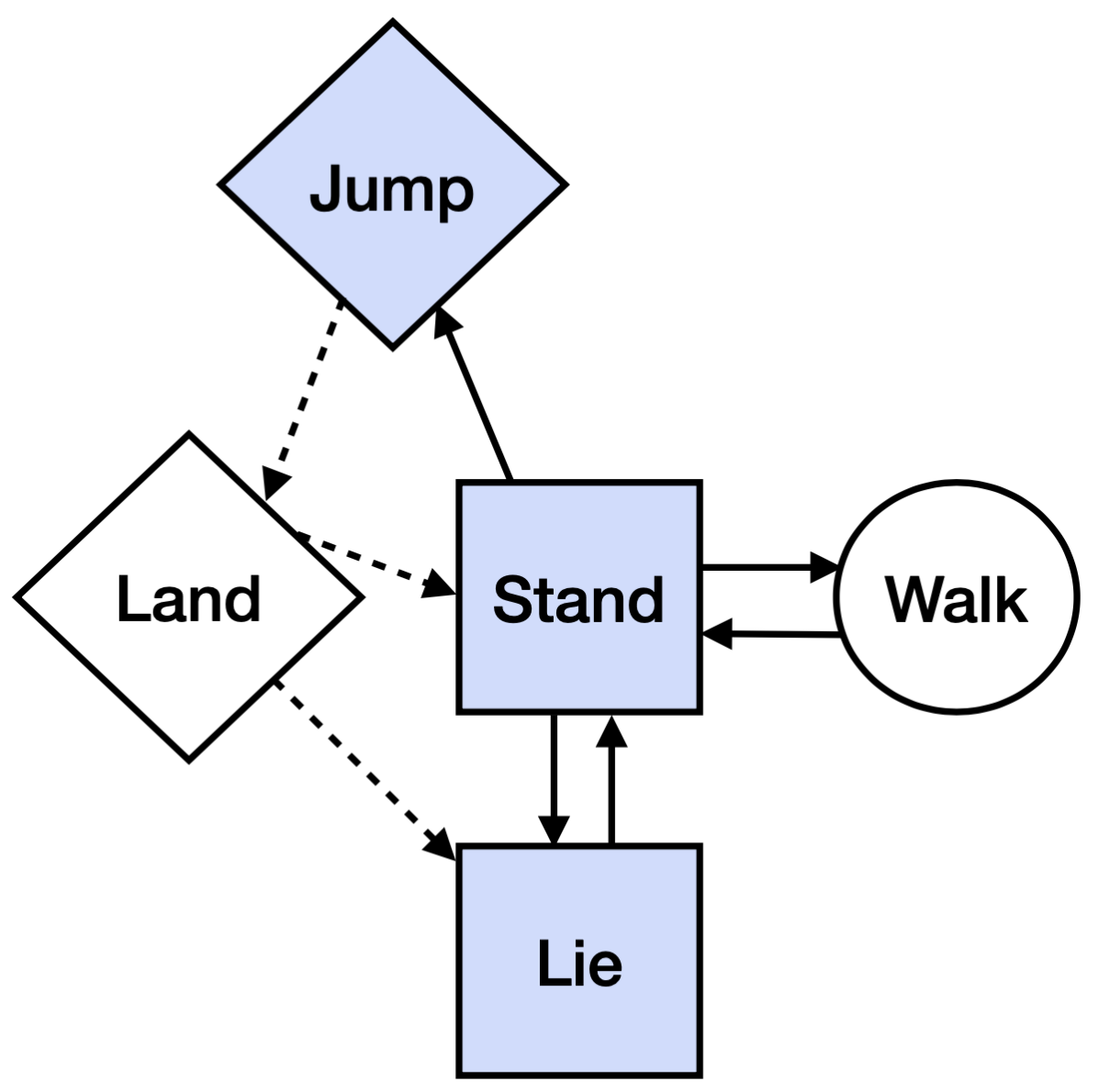
(a) Motion primitive graph.

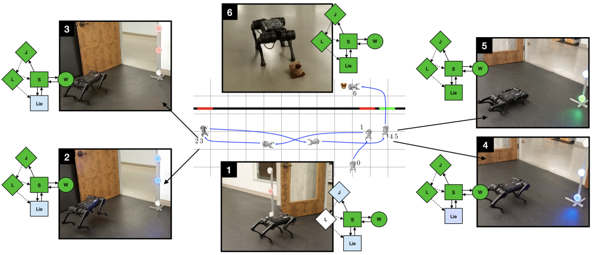
(b) Snapshots of the hardware test execution on the Unitree A1 quadruped.

Figure 3: Resulting test execution on the Unitree A1 quadruped generated by this framework.

IV Experimental Results

We have implemented and validated this framework on simulated grid world examples and hardware experiments. In addition to these examples we have implemented the algorithm on grid world mazes and road networks: the results can be found in this GitHub repository.

IV-1 Robot in a Corridor

The agent under test for the running example is controlled by a simple grid world controller synthesized using TuLiP (Temporal Logic and Planning Toolbox) [32]. The algorithm presented in section III-D results in a test execution during which the system under test visits the two pre-determined key locations before reaching one of the goal states at the end of the corridor. The resulting test execution is shown in Figure 2.

IV-2 Hardware Experiments with Quadruped

Next we will find a test strategy to test an actual robotic system, the Unitree A1 quadruped. This quadruped is controlled using a motion primitive layer with behaviors for lying down, standing, walking, and jumping. The underlying dynamics of the transitions between primitives are abstracted away from the higher-level autonomy as described in [33], and can be commanded directly. The autonomy layer is provided by a TuLiP controller generated on an abstraction of the transition system of the quadruped, consisting of grid world locations and states corresponding to the available motion primitives. We find test strategies and execute the resulting test for two test specifications inspired by a search and rescue mission.

Beaver Rescue

The quadruped’s task is to rescue the beaver from the hallway and return it to the lab, the system specification is given as $\varphi_{\text{sys}}=\lozenge\text{goal}$, where goal corresponds to the quadruped and the beaver reaching the safe location in the lab. The test specification is given as $\varphi_{\text{test}}=\lozenge\text{door}_{1}\land\lozenge\text{door}_{2}$ ensuring that the quadruped will use a different door on the way to the beaver and back into the lab. The resulting test execution shows the quadruped using door 2 to exit the lab into the hallway, after it reaches the beaver this door is shut and the quadruped walks to door 1 and returns the beaver to the safe location in the lab. Snapshots of this test execution can be seen in Figure 1.

Search and Rescue: Motion Primitive Testing

In this test we want to test the motion primitives of the quadruped shown in figure 3. The goal for the quadruped is reaching the beaver in the hallway. The test specification is given as $\varphi_{\text{test}}=\lozenge\text{jump}\land\lozenge\text{lie}\land\lozenge\text{stand}$, which ensures that we will test each of these motion primitive at least once. The test setup includes lights at different heights, which correspond to the motion primitive which might unlock the door. The light starts in blue and after the motion primitive has been executed, the light will turn red - if the door remains locked - or green - if the door is unlocked. Our framework will decide whether the doors will be locked or unlocked according to which motion primitives have already been observed during the test. Snapshots of the test execution are shown in Figure 3.

V Conclusions and Future Work

We outlined the problem of finding the minimally constrained test as a bilevel optimization. For future work, we would like to prove that our algorithm is sound and complete, and provide sub-optimality guarantees on the generated test environment. The approach outlined in this paper requires reactive placement of obstacles during a test, which can be challenging for real-world use cases. Therefore, we aim to extend this framework to include dynamic test agents to constrain the system actions, and also allow for finding test environments requiring the minimum number of test agents to constrain a test environment for a test specification.

References

- [1] S. Sankaranarayanan and G. Fainekos, “Falsification of temporal properties of hybrid systems using the cross-entropy method,” in Proceedings of the 15th ACM international conference on Hybrid Systems: Computation and Control, 2012, pp. 125–134.
- [2] J. Kapinski, J. V. Deshmukh, X. Jin, H. Ito, and K. Butts, “Simulation-based approaches for verification of embedded control systems: An overview of traditional and advanced modeling, testing, and verification techniques,” IEEE Control Systems Magazine, vol. 36, no. 6, pp. 45–64, 2016.
- [3] Y. Annpureddy, C. Liu, G. Fainekos, and S. Sankaranarayanan, “S-taliro: A tool for temporal logic falsification for hybrid systems,” in International Conference on Tools and Algorithms for the Construction and Analysis of Systems. Springer, 2011, pp. 254–257.
- [4] G. Chou, Y. E. Sahin, L. Yang, K. J. Rutledge, P. Nilsson, and N. Ozay, “Using control synthesis to generate corner cases: A case study on autonomous driving,” IEEE Transactions on Computer-Aided Design of Integrated Circuits and Systems, vol. 37, no. 11, pp. 2906–2917, 2018.
- [5] T. Dang and T. Nahhal, “Coverage-guided test generation for continuous and hybrid systems,” Formal Methods in System Design, vol. 34, no. 2, pp. 183–213, 2009.
- [6] M. Hekmatnejad, B. Hoxha, and G. Fainekos, “Search-based test-case generation by monitoring responsibility safety rules,” arXiv preprint arXiv:2005.00326, 2020.
- [7] E. Plaku, L. E. Kavraki, and M. Y. Vardi, “Falsification of ltl safety properties in hybrid systems,” International Journal on Software Tools for Technology Transfer, vol. 15, no. 4, pp. 305–320, 2013.
- [8] A. Donzé, “Breach, a toolbox for verification and parameter synthesis of hybrid systems,” in International Conference on Computer Aided Verification. Springer, 2010, pp. 167–170.
- [9] G. E. Fainekos and G. J. Pappas, “Robustness of temporal logic specifications for continuous-time signals,” Theoretical Computer Science, vol. 410, no. 42, pp. 4262–4291, 2009.
- [10] T. Dreossi, D. J. Fremont, S. Ghosh, E. Kim, H. Ravanbakhsh, M. Vazquez-Chanlatte, and S. A. Seshia, “Verifai: A toolkit for the formal design and analysis of artificial intelligence-based systems,” in International Conference on Computer Aided Verification. Springer, 2019, pp. 432–442.
- [11] “Technical Evaluation Criteria,” https://archive.darpa.mil/grandchallenge/rules.html.
- [12] “DARPA Urban Challenge,” https://www.darpa.mil/about-us/timeline/darpa-urban-challenge.
- [13] H. Kress-Gazit, G. E. Fainekos, and G. J. Pappas, “Temporal-logic-based reactive mission and motion planning,” IEEE transactions on robotics, vol. 25, no. 6, pp. 1370–1381, 2009.
- [14] T. Wongpiromsarn, U. Topcu, and R. M. Murray, “Receding horizon temporal logic planning,” IEEE Transactions on Automatic Control, vol. 57, no. 11, pp. 2817–2830, 2012.
- [15] M. Kloetzer and C. Belta, “Temporal logic planning and control of robotic swarms by hierarchical abstractions,” IEEE Transactions on Robotics, vol. 23, no. 2, pp. 320–330, 2007.
- [16] M. Lahijanian, S. Almagor, D. Fried, L. E. Kavraki, and M. Y. Vardi, “This time the robot settles for a cost: A quantitative approach to temporal logic planning with partial satisfaction,” in Twenty-Ninth AAAI Conference on Artificial Intelligence, 2015.
- [17] A. Censi, K. Slutsky, T. Wongpiromsarn, D. Yershov, S. Pendleton, J. Fu, and E. Frazzoli, “Liability, ethics, and culture-aware behavior specification using rulebooks,” in 2019 International Conference on Robotics and Automation (ICRA). IEEE, 2019, pp. 8536–8542.
- [18] S. Shalev-Shwartz, S. Shammah, and A. Shashua, “On a formal model of safe and scalable self-driving cars,” arXiv preprint arXiv:1708.06374, 2017.
- [19] T. Wongpiromsarn, K. Slutsky, E. Frazzoli, and U. Topcu, “Minimum-violation planning for autonomous systems: Theoretical and practical considerations,” in 2021 American Control Conference (ACC). IEEE, 2021, pp. 4866–4872.
- [20] G. Ernst, P. Arcaini, I. Bennani, A. Donze, G. Fainekos, G. Frehse, L. Mathesen, C. Menghi, G. Pedrinelli, M. Pouzet et al., “Arch-comp 2020 category report: Falsification,” EPiC Series in Computing, 2020.
- [21] S. Ghosh, F. Berkenkamp, G. Ranade, S. Qadeer, and A. Kapoor, “Verifying controllers against adversarial examples with bayesian optimization,” in 2018 IEEE International Conference on Robotics and Automation (ICRA). IEEE, 2018, pp. 7306–7313.
- [22] A. Zutshi, J. V. Deshmukh, S. Sankaranarayanan, and J. Kapinski, “Multiple shooting, cegar-based falsification for hybrid systems,” in Proceedings of the 14th International Conference on Embedded Software, 2014, pp. 1–10.
- [23] A. Corso, R. Moss, M. Koren, R. Lee, and M. Kochenderfer, “A survey of algorithms for black-box safety validation of cyber-physical systems,” Journal of Artificial Intelligence Research, vol. 72, pp. 377–428, 2021.
- [24] J. B. Graebener, A. Badithela, and R. M. Murray, “Towards better test coverage: Merging unit tests for autonomous systems,” in NASA Formal Methods: 14th International Symposium, NFM 2022, Pasadena, CA, USA, May 24–27, 2022, Proceedings, 2022, pp. 133–155.
- [25] A. Badithela, J. B. Graebener, and R. M. Murray, “Minimally constrained testing for autonomy with temporal logic specifications,” 2022.
- [26] C. Baier and J.-P. Katoen, Principles of model checking. MIT press, 2008.
- [27] J. R. Büchi, On a Decision Method in Restricted Second Order Arithmetic. New York, NY: Springer New York, 1990, pp. 425–435. [Online]. Available: https://doi.org/10.1007/978-1-4613-8928-6_23
- [28] O. Kupferman, G. Vardi, and M. Y. Vardi, “Flow games,” in 37th IARCS Annual Conference on Foundations of Software Technology and Theoretical Computer Science (FSTTCS 2017). Schloss Dagstuhl-Leibniz-Zentrum fuer Informatik, 2018.
- [29] T. H. Cormen, C. E. Leiserson, R. L. Rivest, and C. Stein, Introduction to algorithms. MIT press, 2009.
- [30] V. V. Vazirani, Approximation algorithms. Springer, 2001, vol. 1.
- [31] D. Goktas and A. Greenwald, “Convex-concave min-max stackelberg games,” Advances in Neural Information Processing Systems, vol. 34, 2021.
- [32] T. Wongpiromsarn, U. Topcu, N. Ozay, H. Xu, and R. M. Murray, “Tulip: a software toolbox for receding horizon temporal logic planning,” in Proceedings of the 14th international conference on Hybrid systems: computation and control, 2011, pp. 313–314.
- [33] W. Ubellacker, N. Csomay-Shanklin, T. G. Molnar, and A. D. Ames, “Verifying safe transitions between dynamic motion primitives on legged robots,” in 2021 IEEE/RSJ International Conference on Intelligent Robots and Systems (IROS), 2021, pp. 8477–8484.