Computational pathology in renal disease: a comprehensive perspective

Abstract

Computational pathology is a field that has complemented various subspecialties of diagnostic pathology over the last few years. In this article we briefly analyze the different applications in nephrology. We begin by providing an overview of the different forms of image production. We continue by describing the most frequent applications of computer vision models, the salient features of the different clinical applications, and the data protection considerations encountered. We finished the development, delving into the interpretability of these applications, expanding in depth the three dimensions of this area.

I Introduction

Thanks to the expanding research in artificial intelligence, especially computer vision, computational pathology applications have increased considerably in recent years.

Digital pathology can be defined as the process or set of processes by which slides with already processed samples are digitized. Digitizing implies transferring the image that is observed in a light microscope to an image file[1]. These files are called WSI (Whole Slide Image) and have a characteristic that makes them essential for use in pathology: they store different levels of magnification in the same file. This type of configuration is called a pyramid and it allows to optimize the visualization and exploration of the image, by allowing macroscopic exploration at very low levels of magnification and then going to the detail of interest by increasing the magnification[2, 3, 4]. The WSI can be stored on physical servers located in the same hospital or can be stored in cloud storage systems. Its storage has allowed the interconsultation of the same case between several pathologists from different parts of the world, considerably expanding the accuracy of the diagnosis in complex cases[5, 6, 4].

It can be said that digital pathology ends with the digitization of the slide and its storage in the cloud or the physical server[1]. Part of the extension of the definition of digital pathology, recently includes the remote consultation of cases between several institutions from different physical locations in real time[6]. On the other hand, computational pathology includes all those projects and/or prototypes where WSI images are used as a dataset and machine learning or artificial vision algorithms are employed[7, 8, 4]. Computational pathology does not include the use of scanners, or microscopes, or the implementation of molecular biology laboratory procedures. In this discipline, we already have the images stored, which have the authorization of the ethics committee of the donor institutions and, if the case warrants, the informed consent of the patients to whom they belong[9]. Computational pathology also includes digital modification of WSIs (cropping, alignment, contrast, brightness, color channels, color normalization, etc.[10]) and clinical data capture by aligning WSIs with electronic health records[4].

II Data workflow

The data workflow in digital pathology can take many forms. However, the main skeleton is more or less homogeneous in different countries, health networks, hospitals and laboratories. We can begin to describe it by naming its first part: data acquisition. As we have already seen in other publications, data acquisition begins with the capture of the image by the scanner, once the sample is treated and prepared following the determined protocol (for example, H&E). That captured image must be temporarily stored and then reviewed by a qualified professional to determine if the quality is correct for diagnosis (focus and tissue area). This verification is usually done with the help of the barcode (linear or 2D) that identifies the sample and attaches it to the patient’s file. Once the image is verified as correct (without interpreting the diagnostic), the storage of the image is moved to a permanent physical or virtual disk. If the disk is physical, the storage server may be located in the same hospital or in the same laboratory. If the server is virtual, the host system can be in the same country or in a different country. Now, at the moment of establishing the diagnosis (interpreting the image), using it for a virtual consultation (let it be interpreted by another professional pathologist in another place) or when an algorithm analyzes it autonomously, the image must be made available[4].

For this, a transmission of the file must be generated and a deposit of the same (copy) in another physical place or a read-only link can be generated, without the need for file exchange.

III Article structure

In this article, a general review will be made of the current state of computational pathology in the field of nephrology. For this, the techniques used to produce images in renal pathology will be described first with their specific examples. Then, the most common tasks in computational pathology focused on renal pathology will be delved into. Some important details for training automation and data protection will be also analyzed. Finally, the interpretability in the field of images, computational pathology and computational pathology applied to renal pathology will be shown and discussed in depth. Therefore, the article will have the following structure:

1. Workflow in renal disease

2. Light microscopy (LM)

3. Immunoflourescence (IF)

4. Immunohistochemistry (IHC)

5. Electron microscopy (EM)

6. Hyperspectral imagery (HI)

7. Renal computational pathology

8. Frequent use cases in renal computational pathology

9. Image aligning

10. Data protection in renal computational pathology

11. Interpretability

12. First dimension: data level interpretability

13. Second dimension: classification level interpretability

14. Third dimension: model level interpretability

15. Final considerations

IV Workflow in renal disease

After obtaining the sample by renal biopsy, there are three usual types of microscopy techniques that are applied to generate pathology images for diagnosis: light microscopy, immunofluorescence, and electron microscopy.

V Light microscopy (LM)

In light microscopy, the tissue sample obtained must first be fixed to eliminate metabolic activity. In a series of consecutive steps, non-structural contents such as water will be replaced with various substances. Finally, by adding a structure that provides rigidity, fine slices will be cut. On these slices, the staining protocols will be carried out and the dyes will adhere differentially to the cellular structures. Specifically for renal pathology, firstly, after obtaining the sample, it must be processed through the implementation of formaldehyde buffer and paraffin embedding. Subsequently, fine deparaffinized slices will be obtained and subjected to the following stains: periodic acid-silver methenamine, Masson’s trichrome, periodic acid-Schiff, and hematoxylin and eosin[11].

V-A Periodic acid-silver methenamine

This technique is one of those used in nephropathology. The periodic acid of this stain oxidizes the carbohydrates present in the basement membranes of the sample, producing aldehydes. These aldehydes then reduce the silver to visible metallic silver[12].

V-B Masson’s trichrome

This technique combines, as the name indicates, three colors to differentiate structures. In this way, the structures can be separated into[13]:

• Light blue: basement membranes and mesangial matrix.

• Dark blue: collagen.

• Rust-colored:

  • Finely granulated: cytoplasm of endothelial and mesangial cells.

  • Coarsely granulated: cytoplasm of epithelial cells.

• Orange: proteins.

• Red: fibrin.

• Dark brown: nuclei.

V-C Periodic acid-Schiff

This technique also makes it possible to clearly distinguish the basement membranes, which stain bright pink, and the cell nuclei, which stain purple-blue[12].

V-D Hematoxylin and eosin

This technique, the most widespread and common in medical pathology, stains cell nuclei purple-blue (hematoxylin) and the cytoplasm and basement membranes pink (eosin)[12].

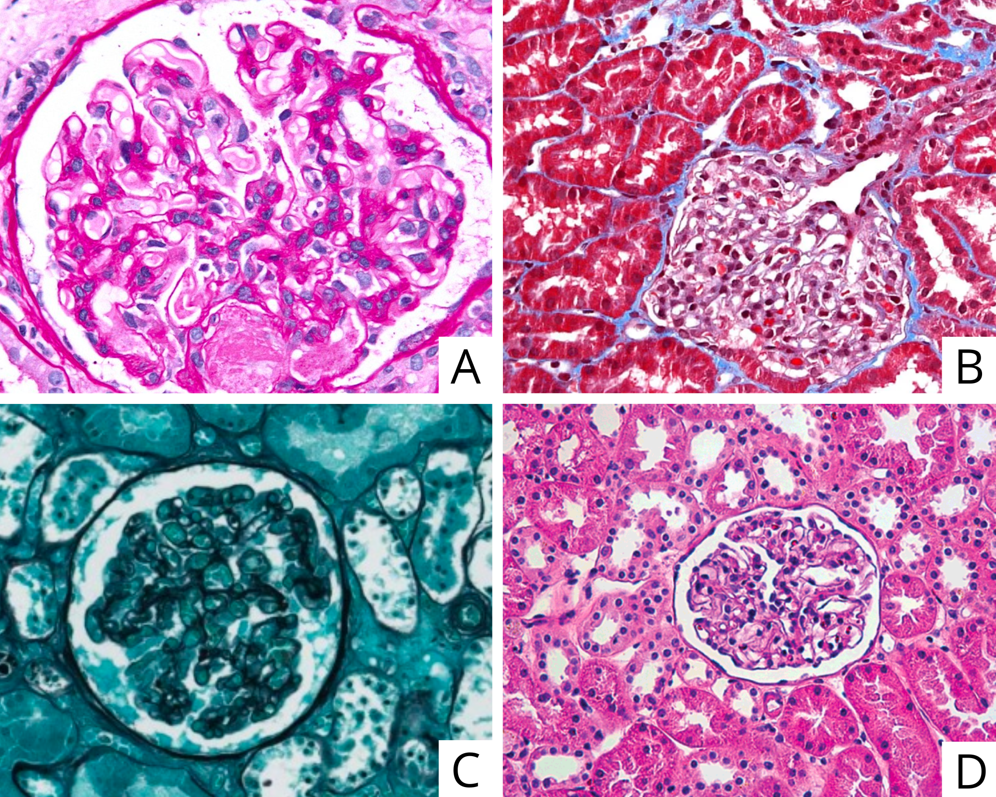
Figure 1: Examples of different stainings of a Bowman’s capsule in kidney biopsies. A, renal cortex taken from a patient with acute thrombotic microangiopathy stained with Periodic acid-Schiff[14]; B, normal renal cortex stained with Mason’s trichrome[15]; C, normal renal cortex stained with periodic acid-silver methenamine[15]; D normal renal cortex stained with hematoxilin and eosin[16].

VI Immunoflourescence (IF)

In immunofluorescence, unlike common histology, the stains are antibodies that adhere to target biomolecules (antigen) identifying a particular tissue portion. The antibodies contain a fluorophore, which after being incubated with the target, bind specifically to it. After incubation, the samples are observed under a fluorescence microscope, which excites the fluorophore with a laser. The fluorophore, after excitation, will return the energy taken from the laser in the form of light of a certain wavelength. Finally this light will be captured by a sensor in the microscope, processed and digitally built in the form of an image. In the specific case of immunofluorescence applied to nephropathology, we have two general approaches.

VI-A Direct immunoflourescence (DIF)

The most widespread and oldest is DIF, which is performed directly from a tissue sample prepared for this specific purpose: frozen tissue. It is important to note that in order to execute this approach, planning must be carried out in advance of the patient’s biopsy and the necessary precautions must be taken to avoid the degradation of the sample during handling.

VI-B Immunofluorescence on paraffin embedded biopsies (PIF)

Many times it is not possible to have frozen tissue for various reasons. Firstly, because it could be not established at the time of the biopsy to carry out a diagnosis by immunofluorescence. Secondly, because the samples have been stored for a long time and are not suitable for the procedure. Or thirdly, simply because it is an interconsultation from another hospital where it is not possible to send a frozen sample by mail[17]. In these cases, it is possible to resort to carrying out immunofluorescence from a paraffin block. It is important to note that paraffin induces protein crosslinking in the sample, which blocks the binding of antibodies to antigens. Therefore, the paraffin sample must be subjected to a process called antigen retrieval, in which proteolytic enzymes (trypsin, proteinase K or pronase E) or heat can be used to disentangle the protein network. Once the antigens have been exposed, the immunofluorescence protocol can be carried out[18]. Although this technique began as a backup for moments when frozen tissue was not available, something crucial was discovered about antigen retrieval. This process succeeded in unmasking antigens in some particular samples that were negative in DIF. That is, antigens that were not seen in the direct technique could only be observed through the previous step in paraffin[19]. In this way, PIF was established as a technique of additional diagnostic value, in addition to being a support for case consultations without frozen tissue samples[17, 19].

VI-C Antibodies for renal pathology

The usual routine antibodies that are usually implemented in renal pathology for immunofluorescence are:

• Heavy chains: IgA (Fig. 2A), IgG (Fig. 2C) and IgM.

• Light chains: Kappa (Fig. 2D) and Lambda (Fig. 2B).

• Complement: C3 and C1q.

• Cellular components: Fibrinogen and Albumin.

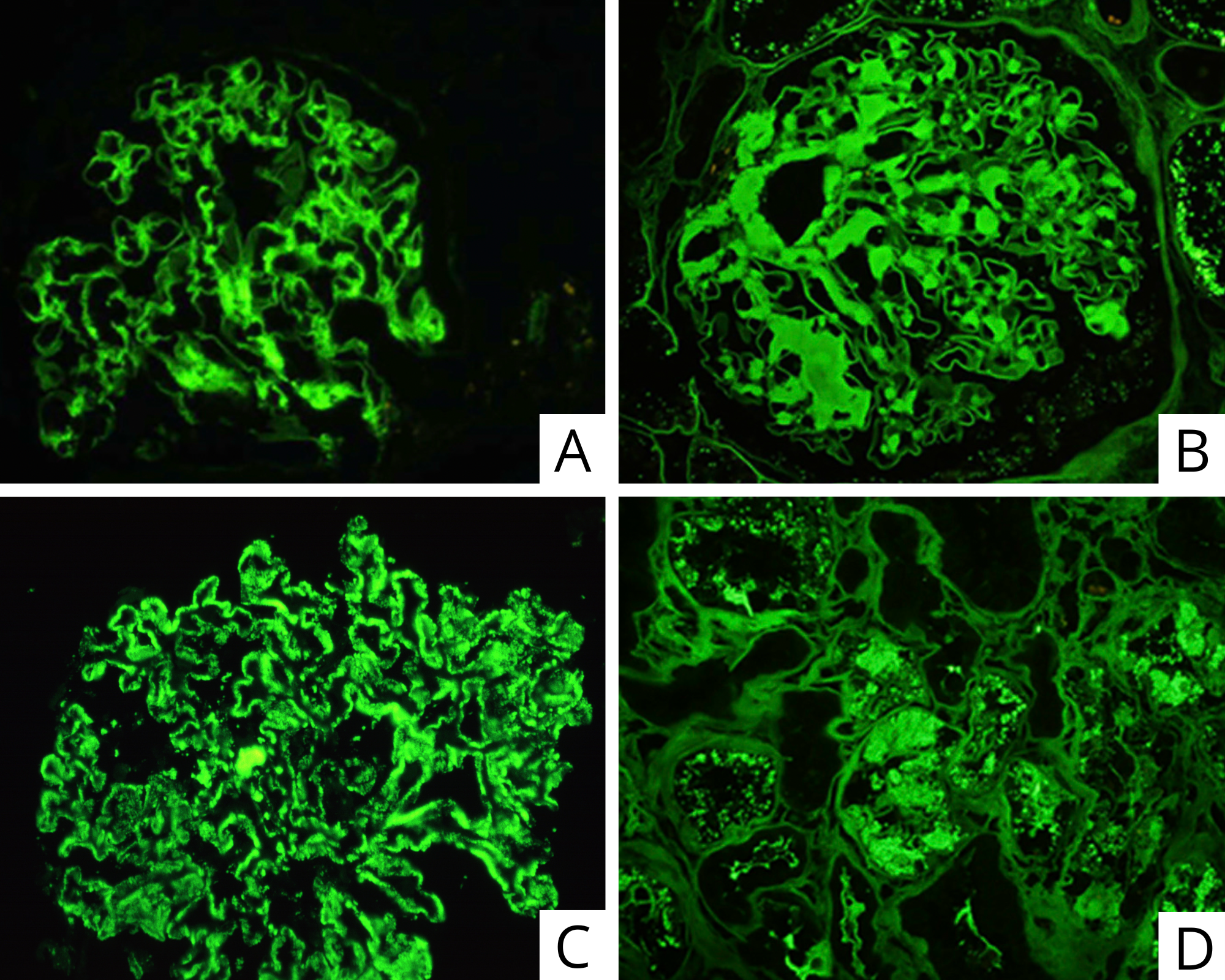
Figure 2: Examples of DIF and PIF images in kidney biopsies. A, PIF of renal cortex taken from a patient with IgA nephropathy, with antibodies against IgA[20]; B, PIF of renal cortex taken from a patient with lambda-type AL amyloidosis, with antibodies against lambda[20]; C, DIF of renal cortex taken from a patient with membranous lupus nephritis, with antibodies against IgG[21]; D, PIF of renal cortex of a patient with kappa-type light chain proximal tubulopathy, with antibodies against kappa[20].

VII Immunohistochemistry (IHC)

In IHC we use the same principle of specific binding between antibodies and antigens as in immunofluorescence. The difference is that in this procedure, the antibody is conjugated with an enzyme (for example, peroxidase) that catalyzes the color change of a substrate. In the specific case of peroxidase, the primary substrate is colorless and after the reaction, it turns brown[22, 23].

In the specific case of kidney disease, this technique is used to identify tumor markers. Within the tumors found in nephrectomies we can find renal cell carcinomas (clear cell, papillary and chromophobes) and also oncocytomas. Among the markers usually studied with IHC, we find[22, 24, 23]:

• Cytokeratin: identification of mainly renal cell carcinoma.

• Vimentin: identification of mainly renal cell carcinoma, clear cell and papillary (Fig. 3).

• Transcription factors PAX8 and PAX9: identification of mainly renal cell carcinoma.

• Renal cell carcinoma marker: identification of mainly renal cell carcinoma.

• CD10: identification of mainly renal cell carcinoma (clear cell and papillary)

• CD9: identification of renal cell carcinoma, chromophobe (Fig. 3).

• Cadherins E and kidney-specific: identification of mainly renal cell carcinoma (chromophobe ) and oncocytomas.

• Parvalbumin: identification of renal cell carcinoma (chromophobe) and oncocytomas.

• Claudins 7 and 8: identification of renal cell carcinoma (chromophobe) and oncocytomas.

• CD117: identification of renal cell carcinoma (chromophobe) and oncocytomas.

• Alpha-Methylacyl Coenzyme A Racemase (AMCAR): identification of renal cell carcinoma (papillary).

• Transcription factors TFE3 and TFEB: mainly involved in pediatric renal cell carcinomas. TFE3 associated with a translocation that involves Xp11.2.

• Cathepsin-K: identification of renal cell carcinoma products of translocations.

• Uroplakin III: identification of renal cell carcinoma of high grade.

• p63: identification of renal cell carcinoma of high grade.

• Thrombomodulin: identification of renal cell carcinoma of high grade.

• GATA3: identification of renal cell carcinoma of high grade.

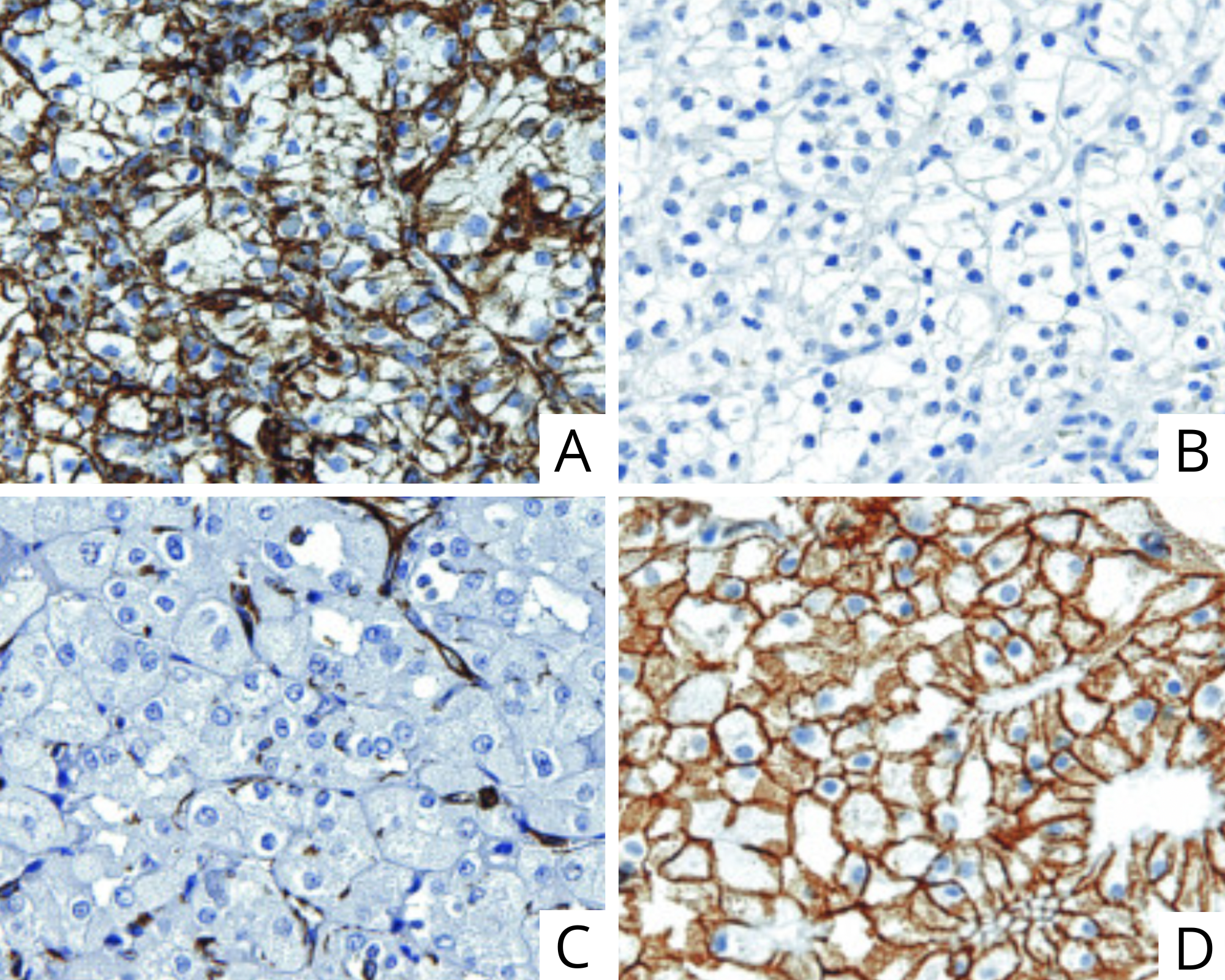
Figure 3: Examples of IHC in renal cell carcinoma (RCC) to separate clear cell subtype from chromophobe[25]. A, clear cell RCC with IHC against Vimentin; B clear cell RCC with IHC against CD9; C, chromophobe RCC with IHC against Vimentin; D, chromophobe RCC with IHC against CD9.

VIII Electron microscopy (EM)

In renal pathology, EM is a necessary partner to diagnose a large number of cases, where the resolution of optical microscopy is not sufficient. In different applications of nephropathology, percentages of cases have been reported where EM adds relevant information for diagnosis (Table I). Of those case reports where EM was necessary, the mean was 49%. This means that from the previous publications, which covered from 1997 to 2020, in 50% of the cases of nephropathology it was necessary to resort to EM to reach the diagnosis. Within renal pathologies, there is a group of them[26] that require the resolution of electron microscopy in order to arrive at a diagnosis (Table II) For example, in cases such as focal segmental glomerulosclerosis, being able to determine the degree and extent of foot process effacement by EM is key to distinguishing between a primary or secondary condition ((Table II). Additionally, of the conditions listed, there are 6 that have one or more associated genes. These pathologies (Fabry, Nail-Patella, trans-retinein amyloidosis, fibronectin glomerulopathy, Alport’s and thin basement membrane) also have confirmation by genetic sequencing that can help determine the diagnosis without necessarily having to resort to EM. However, to stage the progress of those pathologies, it is necessary to have the microscopic image.

VIII-A Procedure

The general protocol for processing kidney biopsies for EM begins with the division of the specimen into 0.5 mm portions and then fixation with 3% glutaraldehyde and osmium tetroxide. Subsequently, the sample must be dehydrated and embedded with SPI-EPON 812. Once the sample is embedded, slices must be made with a glass blade microtome. Finally, when the slices are produced, they must be stained with uranyl acetate and lead citrate, which, due to their density, will absorb the electrons to a greater extent. According to the type of cells and their content, the citrates will be absorbed differentially, resulting in zones with different concentration (Fig. 4). Among these zones, we are going to have ones with more citrate that will absorb more electrons (darker) and others with less citrate (lighter)[27, 28, 11].

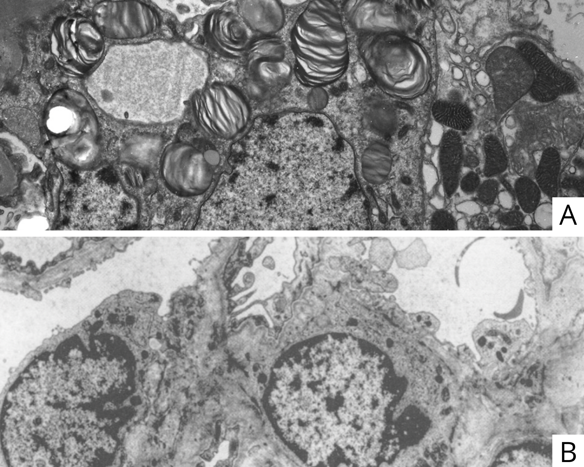
Figure 4: Examples of electron microscopy (EM) images of renal biopsies. A, renal biopsy observed with EM showing zebra bodies of a Fabry disease patient[29]; B, renal biopsy observed with EM showing the enlarged and split glomerular basement membrane (GBM) of an Alport’s syndrome patient[30].

TABLE I: List of publications with the percentage of cases where it was necessary to resort to electron microscopy (EM) for diagnosis in nephropathology.

Application	% of cases	Total cases	Location	Date	Reference
Kidney transplant	50	N/A	Louisiana, USA	1997	[31, 32, 33]
Chronic renal allograft rejection	50	91	Szeged, Hungary	2001	[34]
General nephropathy	72	133	Turku, Finland	2003	[35]
Glomerular disease	38	52	Tunis, Tunisia	2006	[36]
Glomerular disease	20	N/A	Minnesota, USA	2006	[37]
Kidney disease after liver transplant	80	81	New York, USA	2010	[38]
General nephropathy	39	273	Jeddah, Saudi Arabia	2011	[26]
General nephropathy	31	N/A	Kathmandu, Nepal	2013	[39]
Pediatric nephropathy	68	855	Peking, China	2020	[11]

TABLE II: List of renal conditions that require electron microscopy (EM) to be diagnosed. GBM, glomerular basement membrane; BM, basement membrane; FP, foot process; TM, tubules membrane.

Condition	Gene	Microscopic observation	Reference
Fabry	GLA	Zebra bodies / Myelin figures	[40]
Nail-Patella	LMX1B	Zebra bodies / Myelin figures	[41, 42]
Trans retinein amyloidosis	TTR	Amyloid deposits	[43]
Light chain amyloidosis	NO	Amyloid deposits	[43]
Heavy chain amyloidosis	NO	Amyloid deposits	[43]
Serum amyloid A amyloidosis	NO	Amyloid deposits	[43]
Fibrillary glomerulonephritis	NO	Non-branching fibrillary deposits	[44]
Fibronectin glomerulopathy	FN1	Granular and fibrillary deposits	[45]
Collagenofibrotic glomerulopathy	NO	Deposits of collagen bundles	[46]
Alports	COL4A3, COL4A4	Basket-weave pattern	[47, 48]
Thin basement membrane	COL4A3, COL4A4	Diffuse thinning of the GBM	[49]
Diabetic nephropathy	NO	Diffuse thickening of GBM, nonatrophic TM thickened	[50]
Dense deposit disease	NO	Dense transformation of the BM lamina densa	[51]
Minimal change disease	NO	Foot process effacement.	[52]
Focal segmental glomerulosclerosis primary	NO	Extensive foot process effacement	[53]
Focal segmental glomerulosclerosis secondary	NO	Imperceptible FP effacement	[53]
Podocyte infolding glomerulopathy	NO	Intramembranous microspherules, Invagination of FP into GBM	[54]
Transplant glomerulopathy	NO	GBM reduplication	[55]

IX Hyperspectral imagery (HI)

This method consists of capturing multiple planes of information from the tissue sample. The human eye is capable of viewing objects in a wavelength range of 380 to 740 nanometers (nm). Hyperspectral imagery can extend this range to 2500 nm[56]. In this way, the sensor will take multiple snapshots of the same sample at different wavelengths (for example, 400, 450, 500 and 600 nm). This will generate several arrays for each wavelength (Fig. 5, representation of the left). Consequently, each pixel will have information on all the wavelength planes that were recorded. So each pixel will have its own spectrum graph also called spectral signature (Fig. 5, graph on the right)). The spectral signature is simply the representation of the intensity and wavelength recorded in each capture[56, 57]. This method has been applied in the field of pathology, since healthy tissue and pathological tissue present different spectral signatures[58, 57]. This difference is the key to detecting pathological tissue, where a bright field image is not capable of providing information. With regard to applications in renal pathology, thanks to hyperspectral imaging it has been possible to separate and distinguish two membranous nephropathies. In these two highly similar pathologies, one is caused by a virus (hepatitis B virus) and the other is idiopathic[57].

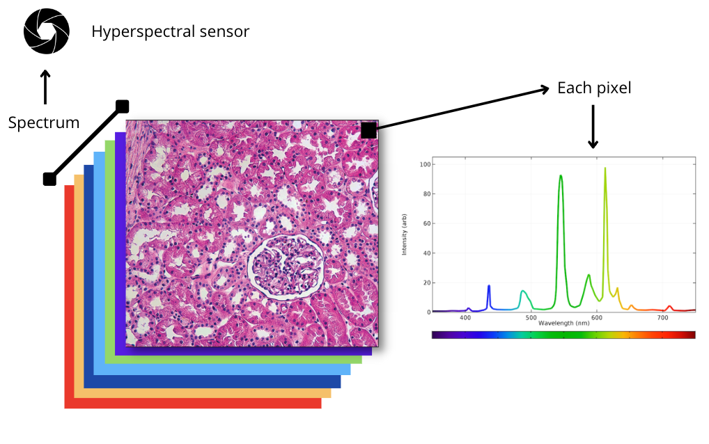
Figure 5: Representation of hyperspectral imagery on kidney tissue. Each color represents a wavelenght and each pixel of the image contains a full spectrum.

IX-A Projection transformation

Since the data of a hyperspectral image is multidimensional, it is advisable to be able to use dimensionality reduction techniques that also help reduce noise. Among the most used we can find the principal component analysis (PCA) or Fisher’s linear discriminant analysis (LDA). These techniques have their negative counterpart, which lies in the need for the data to have a Gaussian distribution. Therefore, there is another technique called local Fisher’s discriminant analysis(LFDA)[57], developed after the previous ones and that does not need a Gaussian distribution to operate.

X Renal computational pathology

In the previous sections we have seen very briefly the different techniques of histology and image acquisition to work in renal pathology. In the next sections, we will inquire about the state of research in computational pathology applied to nephrology.

X-A Common tasks for renal pathology

After a review of the literature, we can agree with the position of the excellent article developed by Huo et al in 2021[59]. The main tasks in which computer vision algorithms are used in renal pathology are:

X-A1 Classification

when we refer to classification in computer vision, we mean to assign a label to an image. In this way, an image enters the algorithm and the algorithm returns a label with a probability (Fig. 6). Given that in pathology, whole slide images (WSIs) have a considerable size, it is customary to partition them into patches. All patches that correspond to a WSI will then be entered into the algorithm. The algorithm will set one label per patch. Then, with all the labels, a heatmap can be made as a visual aid on top of the WSI. A general label of the WSI can also be established (for example, if we identify patches with cancer, the entire WSI will correspond to a cancer patient)[60, 59].

X-A2 Detection

the main difference between classification and detection is that in classification we get only one label in the entire patch. It doesn’t matter if inside this patch there are also other things of interest. However, in detection, in addition to being able to determine several regions of interest in the same area, we can also determine the position. This is especially important in renal pathology, to identify functional units (such as the glomerulus) or to identify anatomical parts (arteries, capillaries or membranes). Within the most used techniques for detection, we find the bounding box(Fig. 6). This technique consists of the creation of an artificial rectangle that identifies the object of interest (for example, the glomerulus[61]) in an image. In this way, the input is the same as in the classification: an image. However the output is different: in detection the output is the image plus the rectangle where the region of interest is[60, 59].

X-A3 Segmentation

when we allude to segmentation, we are alluding to the process of assigning each pixel of an image a particular label. Thanks to knowing exactly how many pixels we have with a certain label, we can perform quantification tasks within an image. For example, in certain neurological diseases it is possible to measure the area within a certain image that is affected and thus determine the diagnosis[62]. In pathology, segmentation is basically used to separate healthy tissue from pathological tissue or to identify functional units (such as the glomerulus)[60]. The segmentation input is an image and the output is a mask(Fig. 6). The mask is superimposable on the image, so it indicates the pixels of interestcite[60, 59].

X-A4 Synthesis

unlike the other three approaches, image synthesis produces new images. To produce these new images, we must first train on the model images. The generator model will learn from the distribution of the training images and will generate new images very similar to the training ones(Fig. 6). However, another model, called a discriminator, will try to discover which are the artificial images within a batch of artificial and real images[63]. This pairing between generator and discriminator will serve to produce in each cycle, artificial images more and more similar to the real ones. In renal pathology, synthesis is used to produce artificial stains. In this way, the network is trained so that it can generate a stain from an image with another stain (for example, H&E to PAS)[60, 59].

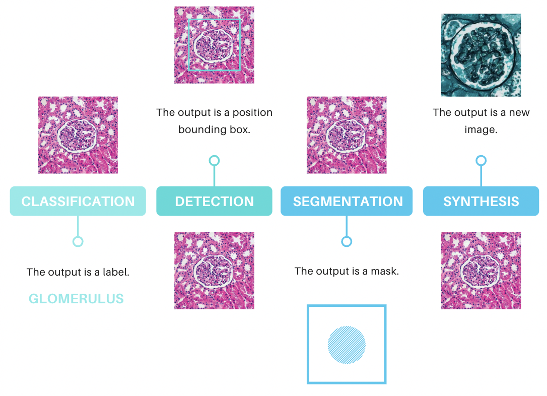
Figure 6: Representation of common tasks in computer vision applied to renal pathology.

XI Frequent use cases in renal computational pathology

After our review of the literature, we can structure and detail some frequent uses of algorithms in renal pathology.

XI-A Glomeruli identification

Of the many research works and prototypes analyzed, there is a large group of them that focus on the identification of glomeruli[61, 64, 65, 66, 67, 68, 69, 70, 71, 72, 73, 74, 75, 76, 77, 78, 79]. This identification can be developed by segmentation[65, 66, 67, 68, 69, 71, 76, 78] or detection[61, 64, 72, 73, 74, 75, 77, 79]. After the recognition of this functional unit, it is possible to proceed to separate pathological from healthy. Also, after this separation, the number of healthy and pathological glomeruli can be quantified, to stage the patient. Of the stains used in these prototypes, we find the most frequent, H&E[61, 64, 66, 70, 71, 72, 77, 79], and also the others typical of renal pathology: PAS[64, 66, 67, 68, 69, 71, 72, 74, 76, 78, 79], PAM[66, 73], Masson[65, 66, 71, 79], Silver[71, 79] and IF[78]. The mean number of patients in these studies was 182, while the study with the largest number had 1281[73] and the one with the least number 10[61]. These prototypes used fliping, rotation, cropping, scaling, contrast and brightness changes, noise adding, transposition and HUE color space transition as data augmentation techniques. Among the most frequent applications of the prototypes we find renal transplantation[61, 67, 69, 75] and the identification of glomerulosclerosis[70, 76, 77].

XI-B Lesion identification

Following a similar reasoning to the one exposed in the previous section, some prototypes focused on the detection of lesions in renal tissue[80, 81, 82, 83]. The most frequent pathology found in this group of studies was IgA nephropathy[80, 82]. Most of the prototypes used PAS-stained[80, 81, 83] images and only one used IF[82].

XI-C Cancer cells identification

Like most of the research papers in oncological digital pathology, a group of the listed papers focused specifically on the identification of tumor cells in renal tissue. Of this group, all were performed in renal cell carcinoma with H&E staining[84, 85, 86, 87]. Two of these works were carried out with images extracted directly from The Cancer Genome Atlas (TCGA)[84, 85].

XI-D Condition identification

Part of the research work was also focused on the identification of specific medical conditions. The techniques used were EM[88], PAS/PAM[89] and IF[90]. One article in particular[88] focused on a group of pathologies such as amyloidosis, diabetic glomerulosclerosis, membranous nephropathy, membrano-proliferative glomerulonephritis and thin basement membrane disease.

XI-E Stain generation

As we mentioned before (Section X-A4), the possibility of generating virtual stains is of vital importance to extend datasets. Two research papers focused on this process. The first of them generating images of Masson trichrome, Jones and PAS from a training with H&E images for the diagnosis of non-neoplastic kidney diseases[91]. Second, IF images are generated from brightfield PAS images, computationally identifying cellular substructures such as cell nuclei, collagen, fibrosis, distal tubules, proximal tubules, endothelial cells and leukocytes[92].

XI-F Individual entities identification

With respect to the identification of individual pathological or functional entities, we have several articles of this type. Among them we find the identification of fibrosis[74], macrophages and lymphocytes[93], deposits[57], peritubular capillaries[94], restricted vascularity[95] and deposits in glomeruli[96]. Other articles instead resort to the segmentation of structures to produce a more accurate pixel map. In this group we find podocyte segmentation[97] and tubule segmentation[98]. Additionally, most of the prototypes that worked on the identification of deposits used some type of immunological technique (IHC or IF)[93, 98, 94, 95]. Also, the only peer-reviewed publication that includes the use of hyperspectral imaging was performed on deposits identification for membranous nephropathy screening[57].

XII Image aligning

One of the biggest challenges in optimizing image labeling work is aligning samples of the same tissue. When performing multiple stains on successive slices of the same surgical specimen, being able to enlarge the image in the same position on all stains is key. Since the images that come from the same surgical piece represent different planes of it, a degree of similarity is expected. However, given the change in plane and the tissue’s own deformation, the differences can be widened. For example, if we are observing a glomerulus in H&E and we want to see if the basement membrane is modified, we can observe that in the PAS image of the same gromerulus. To do this, we would have to locate the gromerulus in the PAS image, which will surely be in another tissue cut plane. There is a technique specifically developed for renal tissue images that allows aligning images of the same surgical piece subjected to successive staining. This technique is called image registration[79]. It consists of grouping images that come from the same origin (surgical piece) and spatially distributing affine transform matrices throughout the extension of each image. These matrices are basically recognition points (tissue characteristics) that are repeated in all the images (Fig. 7). When they have all been identified, they are concatenated in all the images[79]. The recognition points identified above are coordinates. Each coordinate has a unique code. This allows that when an important point is identified in one image (glomerulus in H&E), the same position can be quickly found in another image (glomerulus in PAS).

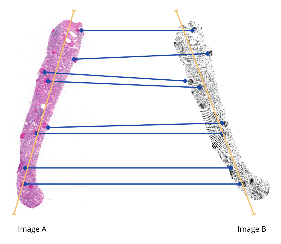
Figure 7: Representation of the image registration process proposed by [79]. Image A, is the first image with one stain. Image B, is the second image with a different stain that come from the same surgical piece. Each blue point represents a coordinate and the blue lines concatenate corresponding points. Yellow lines represent the axis of each image.

XIII Data protection in renal computational pathology

XIII-A Informed consent

Regarding data protection, many articles submitted the justification for the study to the ethics committee of the institution that provided the data (following the Helsinki declaration). The committee itself authorized the execution of the study. It also established the waiver of informed consent justifying that the study was retrospective and does not involve any further tests or treatments of the participants (the samples were already present in the biobank)[80, 74, 75]. Other articles used databases that had already submitted their donors to informed consent for the use of their data. In this way, the authors, as long as they are compliant with the conditions of use of the information and the protection regulations, should not resort to new consents[84, 85, 71]. Some works did not mention in the text of the article or in any appendix if they submitted the study to an ethics committee or if they received an informed consent waiver to proceed with the protocols. It is possible that the information is available in another link or section, which is not directly visible to users[69, 70]. Other studies mention directly in the final statement that they have followed the ethical standards of the Helsinki declaration. However, they do not mention having submitted the protocol to validation by the ethics committee or having had any type of content review by any authority of the partner institution[88].

XIV Interpretability

Interpretability of an algorithm can be defined as a set of protocols, techniques or properties that make the output generation of that algorithm understandable by humans. When we refer to understandable, we mean that it can be inferred, for example, what characteristics of an image were those that defined its belonging to a category (label) in a classification[99].

XIV-A Dimensions of interpretability

It has been proposed that three dimensions could be considered when attempting to interpret the output of an algorithm[99, 100]:

• The first dimension focuses on data. Try to apply techniques to understand which of the dimensions of our data are the most important to solve the task at hand. As we mentioned before (Section XV), the reduction of dimensions and the identification of variables that are correlated can help considerably to select the best features for our model. Having an insight into what features are involved in the task helps us partially understand how a decision is reached.

• The second dimension has to do with prediction. Specifically, how a certain input resulted in a certain output in the algorithm. For example, in an image what angles, silhouettes, shapes or colors are necessary for that image to be classified with a particular label. Examples of this dimension could be CAM (Section XVI-A), GRAD-CAM (Section XVI-B), ablation GRAD-CAM (Section XVI-C) and score CAM (Section XVI-D).

• The third dimension has to do directly with the model. What parts of the model interact with each other and with what force so that the input that enters is processed to a respective output. In the specific case of neural networks, how the layers interact with each other and with what weight the information from a previous layer passes to a later one. Examples of this dimension could be considered activation maximization (Section XVII-1), feature visualization (Section XVII-2) and network dissection (Section XVII-3).

XV First dimension: data level interpretability

When we work with pathology images (WSI), we subject our hardware to a large impact on processing time and number of active units. Therefore, reducing the dimensions of our input data is key to:

• reduce physical storage capacity

• reduce processing time

• increase response speed

When we talk about reducing the dimensions of our data, we are specifically referring to isolating the key information for the task we need to develop. That is, all that part of the information that would not contribute to the task for which the algorithm was built (noise), should disappear. This separation seems simple in words, but it is much more complex in practice[101]. We have several strategies to reduce the dimensions of our data, and we will detail them below.

XV-A Principal component analysis (PCA)

To perform this technique on our features, we must first project the values of those features (for each sample of our dataset) in a space of lower dimension. The type of projection must ensure that the variance of the data is the largest. Having the projected data, we will proceed to search for the main components. These components are vectors that best fit the data. Once we find these small vectors, they will be the components that will represent the thousands of values that previously belonged to these variables[101, 102].

XV-B Gaussian random projection (GRP)

We can also resort to GRP, which simply consists of projecting our features in a space of reduced dimensions. To do this we simply multiply our matrix (features, n x m) by a smaller dimension matrix of random values (m x p) and a scalar (1/square root p). This scalar will help absorb the impact of the pairwise distance resulting from the dimension reduction[101].

XV-C High correlation feature elimination

This method is based on the precept that groups of variables that have a high correlation among them can be represented by only one of the group. In this way, the correlation of each feature with each of its peers must be calculated. If the correlation is greater than a threshold, then one can be kept and the other eliminated. The higher the threshold, the less number of features will be discarded. Therefore, it is important to always perform a finetuning with different thresholds to find the optimal one[101].

XV-D Neural compression

This procedure consists of using the encoder to generate embedded vectors. The encoder is fed with the images whose dimensions we want to reduce. The result will be a vector of reduced dimensions for each image. For WSI, there is a protocol by which the image is divided into patches. Then each patch is converted to a vector. When all the patches have been converted, the image is reassembled with the vectors preserving the location of each one[103, 4].

XV-E t-distributed stochastic neighbor embedding (t-SNE)

t-SNE is a very useful technique for reducing dimensions of multidimensional data. This technique uses the abstract representations (feature vectors) of the last layer of a neural network (before running softmax). Since these vectors are highly multidimensional, this technique reduces the dimensions in a non-linear way. After reduction, it produces a representation of the vectors according to their similarity. This can help us to know, in a multiclass classification, which are the most important features of each class and how similar they are with respect to other classes.

XV-F Applications in renal computational pathology

Of the dimensionality reduction techniques, we find some applications in digital pathology. One group managed to locate the most important features for the classification of different types of nervous system neoplasms, using images similar to those of renal pathology. Moreover, with the t-SNE they managed to represent them visualizing the different types of tumors by similarity[104]. Image compression was very regularly used as a method for dimensionality reduction of pathology images, in breast cancer[103] and lung cancer[105]. H&E images were used in the same fashion as many renal pathology studies. PCA was also used as a color separator in patches of glomeruli, eliminating noise and isolating structural components more effectively than the original image[106]. Regarding the correlation of features, a variation of the method explained above was used to select features correlated with the pathological class. In this way, the features with a correlation coefficient greater than a threshold for the pathological class were selected[107].

XVI Second dimension: classification level interpretability

XVI-A Class Activation Mapping (CAM)

The CAM technique uses the feature maps of the last layer of the neural network. To generate a single usable result, all feature maps are linearly combined using the weights learned from the last layer as a guide. In this way, each feature map is multiplied by its weight and then the linear combination of all of them is produced. An important disadvantage of this technique is the inability to operate with fully connected layers in the last layer. Therefore, the networks that have this characteristic will have to transform their last layer to convolutional and retrain[108].

XVI-B Gradient-weighted Class Activation Mapping (Grad-CAM)

This technique was built using some resources of the previous one. Gradients backpropagating from the output are computed for each class. The weights are calculated from the gradient, using global average pooling. These weights represent, like the previous technique, the importance of each feature map. However, after linearly combining these feature maps with their weights, ReLU is applied. This is the main difference. When applying ReLU, the features that only have a positive influence on the interest class are selected[109, 110].

XVI-C Ablation CAM

Unlike the previous technique, in this one the calculation of the gradient is not made use of. Instead, a process called ablation is employed. To do this, the values of each feature map are set to zero per iteration. The drop in activation score is calculated for the given class, for each of the feature maps. The magnitude of the drop represents the relative importance of each feature map. Finally, following a protocol similar to the previous one, all the calculated importances are combined and ReLU is applied to prioritize only those with a positive effect[111].

XVI-D Score CAM

This technique, like the last one, gets rid of the calculation of the gradient. In this case, as a first step, they generate the feature maps of one of the final layers. As a second step, with these maps, masks are built and applied to the original input. Each new image (mask on input) is passed through the network again. Each pass will generate a score. Finally, all the generated feature maps will be linearly combined (first step) using the scores as weights (second step). ReLU is used at the end of the combination, to take only the positive influence[112].

XVI-E Applications in renal computational pathology

Specifically concerning renal pathology, the most widely used interpretability techniques have been CAM and GradCAM[74, 113]. Regarding the first, it has been used both at the global level of WSI[74] and at the patch level, with a focus on the gromerulus. When multiple pathologies are classified at glomerular level, the focus of the neural network can be seen in the patch. For example, in patients with amyloidosis, the network can be seen focusing on an area of the glomerulus where amyloid deposits are placed[113]. Regarding the technique score CAM, we found only one study that compared its use with respect to GradCAM in the evaluation of renal tissue in patients with immunoglobulin A nephropathy[114]. We can see in the images of the heatmaps, slight differences between one technique and another for the same image and the same class. Regarding dark field images, GradCAM has been applied as well. It has been found that the technique is equally useful and that it is able to point out the regions of importance in the classification, even in digitally blurred images[82].

XVII Third dimension: model level interpretability

XVII-1 Activation maximization

This method aims to find the parts of a certain input (for example, parts of an image) that the network considers to be the most important in order to assign a certain output to that input. In this way, once the model has been trained, this method finds all the features that make up a class. For example, if we train our model with numbers from MNIST, we can generate a list of representations that characterize the label ’8’. This list would contain upper and lower curves that would filter out images resembling a number 8[115]. As we continue with a very particular field, without direct examples in renal computational pathology, we will analyze an example of activation maximization in brain pathology. In this specific case, the filters of layer 159 that most highly activated the neurons for each class were visualized. When analyzing the filters, features were found that corresponded to the type of morphology found[116].

XVII-2 Feature visualization

This research area encompasses a set of techniques and protocols for visualizing features in neural networks. There are a variety of approaches, the main one being optimization to visualize features that can be at the neuron level, at the channel level or at the layer level. Thanks to the optimization, the differences between instances can be interpreted so that two neurons fire together or separately. However, a great challenge in this area, and which extends to all fields of neural networks, is the separation of noise from task-competent information. Especially in feature visualization, we can find representations that are basically noise but that cause neurons to fire in a pattern similar to another image. Being able to identify this and generate representations that make sense is key to being able to interpret an output[117].

XVII-3 Network dissection

This method basically focuses on understanding the behavior of each layer of a neural network. A dataset is used that has different images where each pixel has a particular label (a mask). For example, if we have an image of a garden, all the pixels that correspond to a flower will have a value of 1 and the rest will have a value of 0. Then the activation map of the layer that we want to study is extracted, taking into account that since it is smaller than the input image, we will have to resize it with bilinear interpolation. When we have the activation map with the same size as the input, we compare it with the mask that we generated first. This way we will know what that layer is focusing on. For example, if we have an image with 3 objects (a plate, a glass and a fork), we will have 3 masks. The plate label mask will have values of 1 in all pixels that overlap with the plate. In this way, when we pass the image through the network and obtain the activation map, if it matches better with the plate mask, we will know what is important for the network[118].

XVII-A Applications in renal computational pathology

Given that the third dimension of interpretability is a relatively modern field and its application tells us more about the model than about the model’s task, there are few works applied to Renal computational pathology. One of the works has delved into the features that the model sees when it performs a classification. In addition to having the map of what the model observes, a descriptor has also been incorporated that allows generating a text output on the region of interest (ROI)[119]. The images used have been of H&E histology for urothelial cancer, with a color quite similar to the tumor images of renal samples.

XVIII Final considerations

In the different sections of this article we briefly saw the different partners of renal computational pathology. Starting with the methods for generating images from tissues, we have briefly explored each of them. We have observed the importance of electron microscopy in the diagnosis of renal pathologies. Likewise, we have investigated a relatively new technique such as hyperspectral imaging to further refine the diagnosis of certain pathologies.

In advancing computational pathology methods in nephrology, we have classified the field of computer vision applications. From that classification, we have briefly explored the field of what is published in the area. We have provided an analysis that includes the medical conditions studied, the algorithms, the number of patients and the data augmentation techniques, among other important parameters. We have observed that most of the applications identify primarily the glomerulus. They continue from there in the analysis of that functional unit to detect pathology. Additionally, we have witnessed the possibility of generating new stainings from H&E images using generative adversarial networks (GAN).

As an operational part of the pipelines for computational pathology, we have investigated the techniques for aligning consecutive images (multiple stains) of the same surgical piece. This is extremely useful to speed up the identification of structures in different techniques. For example, correlate IHC markers on H&E images and generate normal and pathological patches.

We have also briefly analyzed the different data protection constraints that different works considered when operating with sensitive patient information. In this particular section we have observed that there is no homogeneous protocol to be followed globally and that many times it is the authors themselves who decide not to submit the research protocol to the review of an institutional ethics committee.

Finally, we have delved into the dimensions of interpretability and its importance in translating the outputs of our models into clinical medical language. Of these dimensions, we have seen how there is a lack of representativeness of the third dimension (model behaviour) not only in renal computational pathology but also in the general computational pathology of the third dimension. Although applications have been exposed in the general field of computer vision, we have found very few works in computational pathology. This could represent an interesting field of research in the future, since it would propose new hypotheses to illuminate the black box that many models represent.

In this appendix we include a table with a brief cataloging and analysis of the relevant publications in Renal computational pathology. The analysis extracts the objective (use) of the algorithms, the medical conditions studied, the type of algorithm, the type of histological staining (image type), the number of patients included in the study, the magnification levels of the images that fed the models, the data augmentation techniques used, the place of origin of the data (data), the geographical location of the institution that developed the work and the bibliographic reference (Table III).

TABLE III: Publication analysis of relevant works in Renal computational pathology. GLR, glomeruli; TU, tubule; AR, artery; FB, fibrosis; RO, rotation; Fl, flip; CON, contrast; CR, crop; COL, color; SCA, scaling; BR, brightness; TRA, transpose; NOI, noise; ELA, elastic deformation; DS, digital staining as augmentation; HUE, hue color space transformation

Use	Conditions	Algorithm	Image type	Patients	Magnification (x)	Augmentations	Data	Location	Year	Reference
GLR detection	Transplant	YOLOv3	HE	10		RO, FL, CON	Hannover Medical School	Germany, France	2020	[61]
GLR detection	N/A	faster R-CNN	HE, PAS	N/A	200, 400	N/A	Taichung Veterans Hospital	Taiwan	2018	[64]
Condition detection	Diabetic nephropathy	CNN	IF	83	N/A	N/A	Okayama University	Japan	2020	[90]
GLR segmentation	Chronic kidney disease	Inception v3 CNN	Masson	171	N/A	NOI	Boston Medical Center	United States	2019	[65]
Condition detection	Global, segmental sclerosis,	InceptionV3	PAS, PAM	283	N/A	N/A	Kyoto University Hospital	Japan	2020	[89]
GLR segmentation	Multiple kidney disease	Cascade Mask R-CNN	HE, PAS, PAM, Masson	664	N/A	RO, FL, CR, TRA	Peking University	China	2021	[66]
GLR segmentation	Transplant	U-Net	PAS	101	200	RO, FL, ELA , SCA, CR, NOI, blur, CON, BR	Radboud Medical Center	Netherlands	2019	[67]
GLR, TU, AR segmentation	Tubulointerstitial nephritis	U-Net	PAS	21	N/A	RO, FL, CON	Kanazawa Hospital	Japan	2022	[68]
Stain generation	Non tumoral renal disease	GAN	HE, PAS, Masson, Jones	58	200	DS	UCLA	United States	2021	[91]
Lesion detection	Ig A nephropathy	LSTM-GCNet, V-Net	PAS	400	400	N/A	Jinling Hospital	China	2020	[80]
GLR, TU, AR, FB segmentation	Transplant	CNN, U-Net	PAS	15	200	RO, TRA, ELA	Radboud Medical Center,	Netherlands	2018	[69]
GLR detecion	Glomerulosclerosis	CNN	HE	17	200	FL, RO, TRA	Washington University	United States	2018	[70]
Cancer cell detection	Renal cell carcinoma	CNN	HE	2093	N/A	FL, CR	The Cancer Genome Atlas	Global	2019	[84]
Cancer cell detection	Renal cell carcinoma	CNN	HE	42	200	N/A	The Cancer Genome Atlas	United States	2020	[85]
GLR segmentation	N/A	U-Net	HE, PAS, Masson, Silver	125	400	N/A	Neptune repository	United States	2021	[71]
GLR detection	N/A	CNN, HOG	HE, PAS, Jones	26	400	N/A	Hannover Medical School	Germany, France	2017	[72]
FB detection	FB	glpathnet	Masson	64	400	N/A	Wexner Medical Center	United States	2021	[74]
GLR detection and classification	Membranous nephropathy	YOLOv3, MIL	PAM	1281	400	N/A	Shanxi Medical University	China	2020	[73]
Stain generation	Transplant	GAN	PAS, IF	20	N/A	N/A	N/A	N/A	2021	[92]
Lesion detection	Transplant	CNN	HE, PAS, Jones	2282	N/A	N/A	Netherland hospitals	Netherlands	2022	[81]
GLR detection and classification	Lupus nephritis	YOLOv4	PAS	163	N/A	FL, RO, SCA, TRA, HUE, NOI	Xijing Hospital	China	2021	[74]
GLR detection	Transplant	Faster R-CNN	N/A	19	N/A	RO	Bari University Hospital	Italy	2020	[75]
GLR and TU segmentation	Glomerulosclerosis	U-Net	PAS	83	100	FL, RO, SCA	Citta della Salute	Italy	2021	[76]
GLR detection	Glomerulosclerosis	VGG16	HE	84	200	FL, RO	Washington University	United States	2021	[77]
Macrophage, lymphocite detection	Transplant	U-Net	IHC	22	N/A	N/A	Hannover Medical School	Germany	2021	[93]
Condition detection	amyloidosis, diabetic glomerulosclerosis	N/A	EM	600	N/A	N/A	Northwell Health	United States	2021	[88]
Interstitium, TUs segmentation	Transplant	R-CNN, U-Net	PAS	93	200	N/A	N/A	United States	2022	[98]
GLR segmentation	Normal tissue	Mask-RCNN	IF, PAS	N/A	N/A	N/A	N/A	United States	2021	[78]
Cancer cell detection	Renal Cell Carcinoma	CNN	HE	44	400	RO, FL, SCA	Louisville Hospital	United States	2022	[86]
Deposition detection	Membranous nephropathy	CNN	Hyperspectral	20	N/A	N/A	China Friendship Hospital	China	2021	[57]
Peritubular capillaries detection	Transplant	CNN	IHC	380	200	RO, FL, SCA	Asan Medical Center	South Korea	2019	[94]
GLR detection	N/A	AlexNet	HE, PAS, Silver, Masson	28	400	N/A	Dartmouth Medical Center	United States	2020	[79]
Vascularity detection	Renal cell carcinoma	SVM	HE, IHC	8	400	N/A	Cedars Medical Center	United States	2017	[95]
Cancer cell detection	Renal cell carcinoma	ResNet	HE	486	200	FL, RO, COL	Dartmouth Medical Center	United States	2021	[87]
Glomerular deposits	N/A	ResNet	IF	2542	400	FL, RO	University of Modena,	Italy	2020	[96]
Lesion detection	IgA, membranous, diabetic nephropathy	AlexNet	IF	1608	N/A	N/A	People’s Liberation Hospital	China	2021	[82]
Podocyte segmentation	Antibody–associated glomerulonephritis	U-Net	IF	317	N/A	N/A	Eschweiler Medical Center	Germany	2021	[97]
Lesion detection	Podocytopathy	VGG19	HE, PAS, PAM	835		FL, RO, BR, SCA	Goncalo Moniz Institute	Brasil	2022	[83]

References

- [1] M. Cui and D. Y. Zhang, “Artificial intelligence and computational pathology,” Laboratory Investigation, vol. 101, no. 4, pp. 412–422, 2021.
- [2] G. Litjens, P. Bandi, B. Ehteshami Bejnordi, O. Geessink, M. Balkenhol, P. Bult, A. Halilovic, M. Hermsen, R. van de Loo, R. Vogels et al., “1399 h&e-stained sentinel lymph node sections of breast cancer patients: the camelyon dataset,” GigaScience, vol. 7, no. 6, p. giy065, 2018.
- [3] M. D. Zarella, D. Bowman, F. Aeffner, N. Farahani, A. Xthona, S. F. Absar, A. Parwani, M. Bui, and D. J. Hartman, “A practical guide to whole slide imaging: a white paper from the digital pathology association,” Archives of pathology & laboratory medicine, vol. 143, no. 2, pp. 222–234, 2019.
- [4] M. Cossio, “Ethereum, ipfs and neural compression to decentralize and protect patient data in computational pathology,” Cambridge Open Engage, 2022.
- [5] M. G. Hanna, O. Ardon, V. E. Reuter, S. J. Sirintrapun, C. England, D. S. Klimstra, and M. R. Hameed, “Integrating digital pathology into clinical practice,” Modern Pathology, vol. 35, no. 2, pp. 152–164, 2022.
- [6] Y. J. Kim, E. H. Roh, and S. Park, “A literature review of quality, costs, process-associated with digital pathology,” Journal of exercise rehabilitation, vol. 17, no. 1, p. 11, 2021.
- [7] E. Abels, L. Pantanowitz, F. Aeffner, M. D. Zarella, J. van der Laak, M. M. Bui, V. N. Vemuri, A. V. Parwani, J. Gibbs, E. Agosto-Arroyo et al., “Computational pathology definitions, best practices, and recommendations for regulatory guidance: a white paper from the digital pathology association,” The Journal of pathology, vol. 249, no. 3, pp. 286–294, 2019.
- [8] A. B. Farris, J. Vizcarra, M. Amgad, L. A. Cooper, D. Gutman, and J. Hogan, “Artificial intelligence and algorithmic computational pathology: an introduction with renal allograft examples,” Histopathology, vol. 78, no. 6, pp. 791–804, 2021.
- [9] T. Sorell, N. Rajpoot, and C. Verrill, “Ethical issues in computational pathology,” Journal of Medical Ethics, vol. 48, no. 4, pp. 278–284, 2022.
- [10] D. Tellez, G. Litjens, P. Bándi, W. Bulten, J.-M. Bokhorst, F. Ciompi, and J. Van Der Laak, “Quantifying the effects of data augmentation and stain color normalization in convolutional neural networks for computational pathology,” Medical image analysis, vol. 58, p. 101544, 2019.
- [11] X. Zhang, J. Xu, H. Xiao, Y. Yao, H. Wang, Y. Ren, M. Liu, F. Wang, X. Zhong, X. Liu et al., “Value of electron microscopy in the pathological diagnosis of native kidney biopsies in children,” Pediatric Nephrology, vol. 35, no. 12, pp. 2285–2295, 2020.
- [12] S. M. Bonsib, Atlas of medical renal pathology. Springer Science & Business Media, 2014.
- [13] A. H. Cohen, “Masson’s trichrome stain in the evaluation of renal biopsies: an appraisal,” American Journal of Clinical Pathology, vol. 65, no. 5, pp. 631–643, 1976.
- [14] K. Benz and K. Amann, “Thrombotic microangiopathy: new insights,” Current opinion in nephrology and hypertension, vol. 19, no. 3, pp. 242–247, 2010.
- [15] S. S. Farouk, R. Hilburg, and M. A. Sparks, “Design, dissemination, and assessment of nephsim: a mobile-optimized nephrology teaching tool,” Journal of graduate medical education, vol. 11, no. 6, pp. 708–712, 2019.
- [16] X. J. Zhou, Z. G. Laszik, T. Nadasdy, and V. D. D’Agati, Silva’s diagnostic renal pathology. Cambridge University Press, 2017.
- [17] G. Singh, L. Singh, R. Ghosh, D. Nath, and A. K. Dinda, “Immunofluorescence on paraffin embedded renal biopsies: Experience of a tertiary care center with review of literature,” World Journal of Nephrology, vol. 5, no. 5, p. 461, 2016.
- [18] S. Zaqout, L.-L. Becker, and A. M. Kaindl, “Immunofluorescence staining of paraffin sections step by step,” Frontiers in neuroanatomy, p. 83, 2020.
- [19] N. C. Messias, P. D. Walker, and C. P. Larsen, “Paraffin immunofluorescence in the renal pathology laboratory: more than a salvage technique,” Modern Pathology, vol. 28, no. 6, pp. 854–860, 2015.
- [20] S. H. Nasr, M. E. Fidler, and S. M. Said, “Paraffin immunofluorescence: a valuable ancillary technique in renal pathology,” Kidney international reports, vol. 3, no. 6, pp. 1260–1266, 2018.
- [21] A. B. Fogo and M. Kashgarian, Diagnostic Atlas of Renal Pathology E-Book. Elsevier Health Sciences, 2021.
- [22] S. S. Shen, L. D. Truong, M. Scarpelli, and A. Lopez-Beltran, “Role of immunohistochemistry in diagnosing renal neoplasms: when is it really useful?” Archives of pathology & laboratory medicine, vol. 136, no. 4, pp. 410–417, 2012.
- [23] H. A. Al-Ahmadie, D. Alden, S. W. Fine, A. Gopalan, K. A. Touijer, P. Russo, V. E. Reuter, and S. K. Tickoo, “Role of immunohistochemistry in the evaluation of needle core biopsies in adult renal cortical tumors: an ex vivo study,” The American journal of surgical pathology, vol. 35, no. 7, pp. 949–961, 2011.
- [24] A. G. Perna, D. A. Ostler, D. Ivan, A. J. Lazar, A. H. Diwan, V. G. Prieto, and J. A. Reed, “Renal cell carcinoma marker (rcc-ma) is specific for cutaneous metastasis of renal cell carcinoma,” Journal of cutaneous pathology, vol. 34, no. 5, pp. 381–385, 2007.
- [25] A. A. Williams, J. Higgins, H. Zhao, B. Ljungberg, and J. D. Brooks, “Cd 9 and vimentin distinguish clear cell from chromophobe renal cell carcinoma,” BMC clinical pathology, vol. 9, no. 1, pp. 1–11, 2009.
- [26] G. A. Mokhtar and S. M. Jallalah, “Role of electron microscopy in evaluation of native kidney biopsy a retrospective study of 273 cases,” 2011.
- [27] D. N. Howell and G. A. Herrera, “Electron microscopy in renal pathology: overall applications and guidelines for tissue, collection, preparation, and stains,” Ultrastructural Pathology, vol. 45, no. 1, pp. 1–18, 2021.
- [28] J. V. Johannessen, “Rapid processing of kidney biopsies for electron microscopy,” Kidney International, vol. 3, no. 1, pp. 46–50, 1973.
- [29] M. Sugarman, J. Choudhury, and A. Jovanovic, “An atypical p. n215s variant of fabry disease with end-stage renal failure,” Molecular Genetics and Metabolism Reports, vol. 15, pp. 43–45, 2018.
- [30] F. Flinter, “Alport’s syndrome.” Journal of medical genetics, vol. 34, no. 4, pp. 326–330, 1997.
- [31] M. Haas, “A reevaluation of routine electron microscopy in the examination of native renal biopsies.” Journal of the American Society of Nephrology, vol. 8, no. 1, pp. 70–76, 1997.
- [32] F. Silva, “Electron microscopic study of medical diseases of the kidney; update-1988,” Modern Pathol, vol. 1, pp. 292–315, 1988.
- [33] G. A. Herrera, J. Isaac, and E. A. Turbat-Herrera, “Role of electron microscopy in transplant renal pathology,” Ultrastructural pathology, vol. 21, no. 6, pp. 481–498, 1997.
- [34] B. Ivanyi, E. Kemeny, E. Szederkenyi, F. Marofka, and P. Szenohradszky, “The value of electron microscopy in the diagnosis of chronic renal allograft rejection,” Modern Pathology, vol. 14, no. 12, pp. 1200–1208, 2001.
- [35] Y. Collan, P. Hirsimäki, H. Aho, M. Wuorela, J. Sundström, R. Tertti, and K. Metsärinne, “Value of electron microscopy in kidney biopsy diagnosis,” Ultrastructural pathology, vol. 29, no. 6, pp. 461–468, 2005.
- [36] S. Darouich, R. L. Goucha, M. H. Jaafoura, F. B. Moussa, S. Zekri, and H. B. Maiz, “Value of electron microscopy in the diagnosis of glomerular diseases,” Ultrastructural pathology, vol. 34, no. 2, pp. 49–61, 2010.
- [37] S. Sethi, M. Haas, G. S. Markowitz, V. D. D’Agati, H. G. Rennke, J. C. Jennette, I. M. Bajema, C. E. Alpers, A. Chang, L. D. Cornell et al., “Mayo clinic/renal pathology society consensus report on pathologic classification, diagnosis, and reporting of gn,” Journal of the American Society of Nephrology, vol. 27, no. 5, pp. 1278–1287, 2016.
- [38] J.-Y. Kim, E. Akalin, S. Dikman, R. Gagliardi, T. Schiano, J. Bromberg, B. Murphy, and G. De Boccardo, “The variable pathology of kidney disease after liver transplantation,” Transplantation, vol. 89, no. 2, pp. 215–221, 2010.
- [39] A. Pant and K. Solez, “The role of electron microscopy in kidney lesions: A review of its diagnostic importance,” Journal of Pathology of Nepal, vol. 3, no. 5, pp. 411–415, 2013.
- [40] P. D. M. de Menezes Neves, J. R. Machado, F. B. Custódio, M. L. G. dos Reis Monteiro, S. Iwamoto, M. Freire, M. F. Ferreira, and M. A. Dos Reis, “Ultrastructural deposits appearing as “zebra bodies” in renal biopsy: Fabry disease?–comparative case reports,” BMC nephrology, vol. 18, no. 1, pp. 1–7, 2017.
- [41] N. Edwards, S. J. Rice, S. Raman, A. M. Hynes, S. Srivastava, I. Moore, M. Al-Hamed, Y. Xu, M. Santibanez-Koref, D. T. Thwaites et al., “A novel lmx1b mutation in a family with end-stage renal disease of ‘unknown cause’,” Clinical kidney journal, vol. 8, no. 1, pp. 113–119, 2015.
- [42] L. Lei, G. Oh, S. Sutherland, G. Abra, J. Higgins, R. Sibley, M. Troxell, and N. Kambham, “Myelin bodies in lmx1b-associated nephropathy: potential for misdiagnosis,” Pediatric Nephrology, vol. 35, no. 9, pp. 1647–1657, 2020.
- [43] S. Nishi, B. Alchi, N. Imai, and F. Gejyo, “New advances in renal amyloidosis,” Clinical and experimental nephrology, vol. 12, no. 2, pp. 93–101, 2008.
- [44] M. A. Lusco, A. B. Fogo, B. Najafian, and C. E. Alpers, “Ajkd atlas of renal pathology: fibrillary glomerulonephritis,” American Journal of Kidney Diseases, vol. 66, no. 4, pp. e27–e28, 2015.
- [45] M. A. Lusco, Y.-p. Chen, H. Cheng, H.-r. Dong, B. Najafian, C. E. Alpers, and A. B. Fogo, “Ajkd atlas of renal pathology: Fibronectin glomerulopathy,” American Journal of Kidney Diseases, vol. 70, no. 5, pp. e21–e22, 2017.
- [46] A. A. Kurien, C. P. Larsen, and L. N. Cossey, “Collagenofibrotic glomerulopathy,” Clinical Kidney Journal, vol. 8, no. 5, pp. 543–547, 2015.
- [47] A. B. Fogo, M. A. Lusco, B. Najafian, and C. E. Alpers, “Ajkd atlas of renal pathology: Alport syndrome,” American Journal of Kidney Diseases, vol. 68, no. 4, pp. e15–e16, 2016.
- [48] C. E. Kashtan, J. Ding, G. Garosi, L. Heidet, L. Massella, K. Nakanishi, K. Nozu, A. Renieri, M. Rheault, F. Wang et al., “Alport syndrome: a unified classification of genetic disorders of collagen iv 345: a position paper of the alport syndrome classification working group,” Kidney international, vol. 93, no. 5, pp. 1045–1051, 2018.
- [49] K. Foster, G. S. Markowitz, and V. D. D’Agati, “Pathology of thin basement membrane nephropathy,” in Seminars in nephrology, vol. 25, no. 3. Elsevier, 2005, pp. 149–158.
- [50] B. Najafian, A. B. Fogo, M. A. Lusco, and C. E. Alpers, “Ajkd atlas of renal pathology: diabetic nephropathy,” American Journal of Kidney Diseases, vol. 66, no. 5, pp. e37–e38, 2015.
- [51] A. B. Fogo, M. A. Lusco, B. Najafian, and C. E. Alpers, “Ajkd atlas of renal pathology: minimal change disease,” American Journal of Kidney Diseases, vol. 66, no. 2, pp. 376–377, 2015.
- [52] ——, “Ajkd atlas of renal pathology: Dense deposit disease,” American Journal of Kidney Diseases, vol. 66, no. 3, pp. e21–e22, 2015.
- [53] ——, “Ajkd atlas of renal pathology: focal segmental glomerulosclerosis,” American Journal of Kidney Diseases, vol. 66, no. 2, pp. e1–e2, 2015.
- [54] J. A. Ting, W. Hung, S. A. McRae, S. J. Barbour, M. Copland, and M. Riazy, “Podocyte infolding glomerulopathy, first case report from north america,” Canadian Journal of Kidney Health and Disease, vol. 8, p. 20543581211048357, 2021.
- [55] E. J. Filippone, P. A. McCue, and J. L. Farber, “Transplant glomerulopathy,” Modern Pathology, vol. 31, no. 2, pp. 235–252, 2018.
- [56] S. Ortega, M. Halicek, H. Fabelo, G. M. Callico, and B. Fei, “Hyperspectral and multispectral imaging in digital and computational pathology: a systematic review,” Biomedical Optics Express, vol. 11, no. 6, pp. 3195–3233, 2020.
- [57] T. Tu, X. Wei, Y. Yang, N. Zhang, W. Li, X. Tu, and W. Li, “Deep learning-based framework for the distinction of membranous nephropathy: a new approach through hyperspectral imagery,” BMC nephrology, vol. 22, no. 1, pp. 1–10, 2021.
- [58] G. M. Callicó, “Image sensors go broadband,” Nature Photonics, vol. 11, no. 6, pp. 332–333, 2017.
- [59] Y. Huo, R. Deng, Q. Liu, A. B. Fogo, and H. Yang, “Ai applications in renal pathology,” Kidney international, vol. 99, no. 6, pp. 1309–1320, 2021.
- [60] I. Goodfellow, Y. Bengio, and A. Courville, Deep learning. MIT press, 2016.
- [61] R. Heckenauer, J. Weber, C. Wemmert, F. Feuerhake, M. Hassenforder, P.-A. Muller, and G. Forestier, “Real-time detection of glomeruli in renal pathology,” in 2020 IEEE 33rd International Symposium on Computer-Based Medical Systems (CBMS). IEEE, 2020, pp. 350–355.
- [62] A. Jose, S. Ravi, and M. Sambath, “Brain tumor segmentation using k-means clustering and fuzzy c-means algorithms and its area calculation,” International Journal of Innovative Research in Computer and Communication Engineering, vol. 2, no. 3, 2014.
- [63] X. Liu, L. Song, S. Liu, and Y. Zhang, “A review of deep-learning-based medical image segmentation methods,” Sustainability, vol. 13, no. 3, p. 1224, 2021.
- [64] Y.-C. Lo, C.-F. Juang, I. Chung, S.-N. Guo, M.-L. Huang, M.-C. Wen, C.-J. Lin, H.-Y. Lin et al., “Glomerulus detection on light microscopic images of renal pathology with the faster r-cnn,” in International Conference on Neural Information Processing. Springer, 2018, pp. 369–377.
- [65] S. Kannan, L. A. Morgan, B. Liang, M. G. Cheung, C. Q. Lin, D. Mun, R. G. Nader, M. E. Belghasem, J. M. Henderson, J. M. Francis et al., “Segmentation of glomeruli within trichrome images using deep learning,” Kidney international reports, vol. 4, no. 7, pp. 955–962, 2019.
- [66] L. Jiang, W. Chen, B. Dong, K. Mei, C. Zhu, J. Liu, M. Cai, Y. Yan, G. Wang, L. Zuo et al., “A deep learning-based approach for glomeruli instance segmentation from multistained renal biopsy pathologic images,” The American Journal of Pathology, vol. 191, no. 8, pp. 1431–1441, 2021.
- [67] M. Hermsen, T. de Bel, M. Den Boer, E. J. Steenbergen, J. Kers, S. Florquin, J. J. Roelofs, M. D. Stegall, M. P. Alexander, B. H. Smith et al., “Deep learning–based histopathologic assessment of kidney tissue,” Journal of the American Society of Nephrology, vol. 30, no. 10, pp. 1968–1979, 2019.
- [68] S. Hara, E. Haneda, M. Kawakami, K. Morita, R. Nishioka, T. Zoshima, M. Kometani, T. Yoneda, M. Kawano, S. Karashima et al., “Evaluating tubulointerstitial compartments in renal biopsy specimens using a deep learning-based approach for classifying normal and abnormal tubules,” PloS one, vol. 17, no. 7, p. e0271161, 2022.
- [69] T. de Bel, M. Hermsen, B. Smeets, L. Hilbrands, J. van der Laak, and G. Litjens, “Automatic segmentation of histopathological slides of renal tissue using deep learning,” in Medical Imaging 2018: Digital Pathology, vol. 10581. SPIE, 2018, pp. 285–290.
- [70] J. N. Marsh, M. K. Matlock, S. Kudose, T.-C. Liu, T. S. Stappenbeck, J. P. Gaut, and S. J. Swamidass, “Deep learning global glomerulosclerosis in transplant kidney frozen sections,” IEEE transactions on medical imaging, vol. 37, no. 12, pp. 2718–2728, 2018.
- [71] C. P. Jayapandian, Y. Chen, A. R. Janowczyk, M. B. Palmer, C. A. Cassol, M. Sekulic, J. B. Hodgin, J. Zee, S. M. Hewitt, J. O’Toole et al., “Development and evaluation of deep learning–based segmentation of histologic structures in the kidney cortex with multiple histologic stains,” Kidney international, vol. 99, no. 1, pp. 86–101, 2021.
- [72] M. Temerinac-Ott, G. Forestier, J. Schmitz, M. Hermsen, J. Bräsen, F. Feuerhake, and C. Wemmert, “Detection of glomeruli in renal pathology by mutual comparison of multiple staining modalities,” in Proceedings of the 10th International Symposium on Image and Signal Processing and Analysis. IEEE, 2017, pp. 19–24.
- [73] F. Hao, M. Li, X. Liu, X. Li, J. Yue, and W. Han, “Classification of glomeruli with membranous nephropathy on renal digital pathological images with deep learning,” in Proceedings of the 2020 Conference on Artificial Intelligence and Healthcare, 2020, pp. 239–243.
- [74] Y. Zheng, C. A. Cassol, S. Jung, D. Veerapaneni, V. C. Chitalia, K. Y. Ren, S. S. Bellur, P. Boor, L. M. Barisoni, S. S. Waikar et al., “Deep-learning–driven quantification of interstitial fibrosis in digitized kidney biopsies,” The American journal of pathology, vol. 191, no. 8, pp. 1442–1453, 2021.
- [75] N. Altini, G. D. Cascarano, A. Brunetti, I. De Feudis, D. Buongiorno, M. Rossini, F. Pesce, L. Gesualdo, and V. Bevilacqua, “A deep learning instance segmentation approach for global glomerulosclerosis assessment in donor kidney biopsies,” Electronics, vol. 9, no. 11, p. 1768, 2020.
- [76] M. Salvi, A. Mogetta, A. Gambella, L. Molinaro, A. Barreca, M. Papotti, and F. Molinari, “Automated assessment of glomerulosclerosis and tubular atrophy using deep learning,” Computerized Medical Imaging and Graphics, vol. 90, p. 101930, 2021.
- [77] J. N. Marsh, T.-C. Liu, P. C. Wilson, S. J. Swamidass, and J. P. Gaut, “Development and validation of a deep learning model to quantify glomerulosclerosis in kidney biopsy specimens,” JAMA network open, vol. 4, no. 1, pp. e2 030 939–e2 030 939, 2021.
- [78] N. H. Patterson, E. K. Neumann, K. Sharman, J. Allen, R. Harris, A. B. Fogo, M. de Caestecker, R. M. Caprioli, R. Van de Plas, and J. M. Spraggins, “Autofluorescence microscopy as a label-free tool for renal histology and glomerular segmentation,” bioRxiv, 2021.
- [79] D. C. Wilbur, J. R. Pettus, M. L. Smith, L. D. Cornell, A. Andryushkin, R. Wingard, and E. Wirch, “Using image registration and machine learning to develop a workstation tool for rapid analysis of glomeruli in medical renal biopsies,” Journal of Pathology Informatics, vol. 11, no. 1, p. 37, 2020.
- [80] C. Zeng, Y. Nan, F. Xu, Q. Lei, F. Li, T. Chen, S. Liang, X. Hou, B. Lv, D. Liang et al., “Identification of glomerular lesions and intrinsic glomerular cell types in kidney diseases via deep learning,” The Journal of pathology, vol. 252, no. 1, pp. 53–64, 2020.
- [81] J. Kers, R. D. Bülow, B. M. Klinkhammer, G. E. Breimer, F. Fontana, A. A. Abiola, R. Hofstraat, G. L. Corthals, H. Peters-Sengers, S. Djudjaj et al., “Deep learning-based classification of kidney transplant pathology: a retrospective, multicentre, proof-of-concept study,” The Lancet Digital Health, vol. 4, no. 1, pp. e18–e26, 2022.
- [82] S. Pan, Y. Fu, P. Chen, J. Liu, W. Liu, X. Wang, G. Cai, Z. Yin, J. Wu, L. Tang et al., “Multi-task learning-based immunofluorescence classification of kidney disease,” International Journal of Environmental Research and Public Health, vol. 18, no. 20, p. 10798, 2021.
- [83] G. O. Barros, D. C. Wanderley, L. O. Rebouças, W. L. dos Santos, A. A. Duarte, and F. de Barros Vidal, “Podnet: Ensemble-based classification of podocytopathy on kidney glomerular images.” in VISIGRAPP (5: VISAPP), 2022, pp. 405–412.
- [84] S. Tabibu, P. Vinod, and C. Jawahar, “Pan-renal cell carcinoma classification and survival prediction from histopathology images using deep learning,” Scientific reports, vol. 9, no. 1, pp. 1–9, 2019.
- [85] M. Fenstermaker, S. A. Tomlins, K. Singh, J. Wiens, and T. M. Morgan, “Development and validation of a deep-learning model to assist with renal cell carcinoma histopathologic interpretation,” Urology, vol. 144, pp. 152–157, 2020.
- [86] H. A. Abdeltawab, F. A. Khalifa, M. A. Ghazal, L. Cheng, A. S. El-Baz, and D. D. Gondim, “A deep learning framework for automated classification of histopathological kidney whole-slide images,” Journal of Pathology Informatics, vol. 13, p. 100093, 2022.
- [87] M. Zhu, B. Ren, R. Richards, M. Suriawinata, N. Tomita, and S. Hassanpour, “Development and evaluation of a deep neural network for histologic classification of renal cell carcinoma on biopsy and surgical resection slides,” Scientific reports, vol. 11, no. 1, pp. 1–9, 2021.
- [88] S. Hacking and V. Bijol, “Deep learning for the classification of medical kidney disease: a pilot study for electron microscopy,” Ultrastructural Pathology, vol. 45, no. 2, pp. 118–127, 2021.
- [89] E. Uchino, K. Suzuki, N. Sato, R. Kojima, Y. Tamada, S. Hiragi, H. Yokoi, N. Yugami, S. Minamiguchi, H. Haga et al., “Classification of glomerular pathological findings using deep learning and nephrologist–ai collective intelligence approach,” International Journal of Medical Informatics, vol. 141, p. 104231, 2020.
- [90] S. Kitamura, K. Takahashi, Y. Sang, K. Fukushima, K. Tsuji, and J. Wada, “Deep learning could diagnose diabetic nephropathy with renal pathological immunofluorescent images,” Diagnostics, vol. 10, no. 7, p. 466, 2020.
- [91] K. de Haan, Y. Zhang, J. E. Zuckerman, T. Liu, A. E. Sisk, M. F. Diaz, K.-Y. Jen, A. Nobori, S. Liou, S. Zhang et al., “Deep learning-based transformation of h&e stained tissues into special stains,” Nature communications, vol. 12, no. 1, pp. 1–13, 2021.
- [92] K.-Y. Jen, L. K. Murali, B. Lutnick, B. Ginley, D. Govind, H. Mori, G. Gao, and P. Sarder, “In silico multi-compartment detection based on multiplex immunohistochemical staining in renal pathology,” in Medical Imaging 2021: Digital Pathology, vol. 11603. SPIE, 2021, pp. 294–301.
- [93] M. Hermsen, V. Volk, J. H. Bräsen, D. J. Geijs, W. Gwinner, J. Kers, J. Linmans, N. S. Schaadt, J. Schmitz, E. J. Steenbergen et al., “Quantitative assessment of inflammatory infiltrates in kidney transplant biopsies using multiplex tyramide signal amplification and deep learning,” Laboratory Investigation, vol. 101, no. 8, pp. 970–982, 2021.
- [94] Y.-G. Kim, G. Choi, H. Go, Y. Cho, H. Lee, A. Lee, B. Park, N. Kim et al., “A fully automated system using a convolutional neural network to predict renal allograft rejection: Extra-validation with giga-pixel immunostained slides,” Scientific reports, vol. 9, no. 1, pp. 1–10, 2019.
- [95] F. Huang, A. Conley, S. You, Z. Ma, S. Klimov, C. Ohe, X. Yuan, M. B. Amin, R. Figlin, A. Gertych et al., “A novel machine learning approach reveals latent vascular phenotypes predictive of renal cancer outcome,” Scientific reports, vol. 7, no. 1, pp. 1–10, 2017.
- [96] G. Ligabue, F. Pollastri, F. Fontana, M. Leonelli, L. Furci, S. Giovanella, G. Alfano, G. Cappelli, F. Testa, F. Bolelli et al., “Evaluation of the classification accuracy of the kidney biopsy direct immunofluorescence through convolutional neural networks,” Clinical Journal of the American Society of Nephrology, vol. 15, no. 10, pp. 1445–1454, 2020.
- [97] M. Zimmermann, M. Klaus, M. N. Wong, A.-K. Thebille, L. Gernhold, C. Kuppe, M. Halder, J. Kranz, N. Wanner, F. Braun et al., “Deep learning–based molecular morphometrics for kidney biopsies,” JCI insight, vol. 6, no. 7, 2021.
- [98] Z. Yi, F. Salem, M. C. Menon, K. Keung, C. Xi, S. Hultin, M. R. H. Al Rasheed, L. Li, F. Su, Z. Sun et al., “Deep learning identified pathological abnormalities predictive of graft loss in kidney transplant biopsies,” Kidney International, vol. 101, no. 2, pp. 288–298, 2022.
- [99] M. Graziani, “Interpretability of deep learning for medical image classification: Improved understandability and generalization,” Ph.D. dissertation, University of Geneva, 2021.
- [100] G. Montavon, W. Samek, and K.-R. Müller, “Methods for interpreting and understanding deep neural networks,” Digital signal processing, vol. 73, pp. 1–15, 2018.
- [101] S. Cascianelli, R. Bello-Cerezo, F. Bianconi, M. L. Fravolini, M. Belal, B. Palumbo, and J. N. Kather, “Dimensionality reduction strategies for cnn-based classification of histopathological images,” in International conference on intelligent interactive multimedia systems and services. Springer, 2018, pp. 21–30.
- [102] C. M. Bishop and N. M. Nasrabadi, Pattern recognition and machine learning. Springer, 2006, vol. 4, no. 4.
- [103] D. Tellez, G. Litjens, J. van der Laak, and F. Ciompi, “Neural image compression for gigapixel histopathology image analysis,” IEEE transactions on pattern analysis and machine intelligence, vol. 43, no. 2, pp. 567–578, 2019.
- [104] K. Faust, Q. Xie, D. Han, K. Goyle, Z. Volynskaya, U. Djuric, and P. Diamandis, “Visualizing histopathologic deep learning classification and anomaly detection using nonlinear feature space dimensionality reduction,” BMC bioinformatics, vol. 19, no. 1, pp. 1–15, 2018.
- [105] W. Aswolinskiy, D. Tellez, G. Raya, L. van der Woude, M. Looijen-Salamon, J. van der Laak, K. Grunberg, and F. Ciompi, “Neural image compression for non-small cell lung cancer subtype classification in h&e stained whole-slide images,” in Medical Imaging 2021: Digital Pathology, vol. 11603. SPIE, 2021, p. 1160304.
- [106] P. Sarder, B. Ginley, and J. E. Tomaszewski, “Automated renal histopathology: digital extraction and quantification of renal pathology,” in Medical Imaging 2016: Digital Pathology, vol. 9791. SPIE, 2016, pp. 112–123.
- [107] L. Shen, W. Sun, Q. Zhang, M. Wei, H. Xu, X. Luo, G. Wang, and F. Zhou, “Deep learning-based model significantly improves diagnostic performance for assessing renal histopathology in lupus glomerulonephritis,” Kidney Diseases, vol. 8, no. 4, pp. 326–335, 2022.
- [108] B. Zhou, A. Khosla, A. Lapedriza, A. Oliva, and A. Torralba, “Learning deep features for discriminative localization,” in Proceedings of the IEEE conference on computer vision and pattern recognition, 2016, pp. 2921–2929.
- [109] R. R. Selvaraju, A. Das, R. Vedantam, M. Cogswell, D. Parikh, and D. Batra, “Grad-cam: Why did you say that?” arXiv preprint arXiv:1611.07450, 2016.
- [110] R. R. Selvaraju, M. Cogswell, A. Das, R. Vedantam, D. Parikh, and D. Batra, “Grad-cam: Visual explanations from deep networks via gradient-based localization,” in Proceedings of the IEEE international conference on computer vision, 2017, pp. 618–626.
- [111] H. G. Ramaswamy et al., “Ablation-cam: Visual explanations for deep convolutional network via gradient-free localization,” in Proceedings of the IEEE/CVF Winter Conference on Applications of Computer Vision, 2020, pp. 983–991.
- [112] H. Wang, Z. Wang, M. Du, F. Yang, Z. Zhang, S. Ding, P. Mardziel, and X. Hu, “Score-cam: Score-weighted visual explanations for convolutional neural networks,” in Proceedings of the IEEE/CVF conference on computer vision and pattern recognition workshops, 2020, pp. 24–25.
- [113] C.-A. Weis, J. N. Bindzus, J. Voigt, M. Runz, S. Hertjens, M. M. Gaida, Z. V. Popovic, and S. Porubsky, “Assessment of glomerular morphological patterns by deep learning algorithms,” Journal of Nephrology, vol. 35, no. 2, pp. 417–427, 2022.
- [114] N. Sato, E. Uchino, R. Kojima, M. Sakuragi, S. Hiragi, S. Minamiguchi, H. Haga, H. Yokoi, M. Yanagita, and Y. Okuno, “Evaluation of kidney histological images using unsupervised deep learning,” Kidney international reports, vol. 6, no. 9, pp. 2445–2454, 2021.
- [115] D. Erhan, Y. Bengio, A. Courville, and P. Vincent, “Visualizing higher-layer features of a deep network,” University of Montreal, vol. 1341, no. 3, p. 1, 2009.
- [116] T. C. Hollon, B. Pandian, A. R. Adapa, E. Urias, A. V. Save, S. S. S. Khalsa, D. G. Eichberg, R. S. D’Amico, Z. U. Farooq, S. Lewis et al., “Near real-time intraoperative brain tumor diagnosis using stimulated raman histology and deep neural networks,” Nature medicine, vol. 26, no. 1, pp. 52–58, 2020.
- [117] C. Olah, A. Mordvintsev, and L. Schubert, “Feature visualization,” Distill, vol. 2, no. 11, p. e7, 2017.
- [118] D. Bau, B. Zhou, A. Khosla, A. Oliva, and A. Torralba, “Network dissection: Quantifying interpretability of deep visual representations,” in Proceedings of the IEEE conference on computer vision and pattern recognition, 2017, pp. 6541–6549.
- [119] Z. Zhang, P. Chen, M. McGough, F. Xing, C. Wang, M. Bui, Y. Xie, M. Sapkota, L. Cui, J. Dhillon et al., “Pathologist-level interpretable whole-slide cancer diagnosis with deep learning,” Nature Machine Intelligence, vol. 1, no. 5, pp. 236–245, 2019.