Nonparametric Quantile Regression: Non-Crossing Constraints and Conformal Prediction

Abstract

We propose a nonparametric quantile regression method using deep neural networks with a rectified linear unit penalty function to avoid quantile crossing. This penalty function is computationally feasible for enforcing non-crossing constraints in multi-dimensional nonparametric quantile regression. We establish non-asymptotic upper bounds for the excess risk of the proposed nonparametric quantile regression function estimators. Our error bounds achieve optimal minimax rate of convergence for the Hölder class, and the prefactors of the error bounds depend polynomially on the dimension of the predictor, instead of exponentially. Based on the proposed non-crossing penalized deep quantile regression, we construct conformal prediction intervals that are fully adaptive to heterogeneity. The proposed prediction interval is shown to have good properties in terms of validity and accuracy under reasonable conditions. We also derive non-asymptotic upper bounds for the difference of the lengths between the proposed non-crossing conformal prediction interval and the theoretically oracle prediction interval. Numerical experiments including simulation studies and a real data example are conducted to demonstrate the effectiveness of the proposed method.

Keywords: Conformal inference; Non-crossing quantile curves; Deep neural networks; Nonparametric estimation; Prediction accuracy

1 Introduction

How to assess uncertainty in prediction is a fundamental problem in statistics. Conformal prediction is a general distribution-free methodology for constructing prediction intervals with a guaranteed coverage probability in finite samples (Papadopoulos et al.,, 2002; Vovk et al.,, 2005). We propose a method for nonparametric estimation of quantile regression functions with the constraint that two quantile functions for different quantile levels do not cross. We then use estimated non-crossing quantile regression functions for constructing conformal prediction intervals.

Since Vovk et al., (2005) formally introduced the basic framework of conformal prediction, there has been a number of important advancements on conformal prediction (Vovk,, 2012; Lei et al.,, 2013; Lei and Wasserman,, 2014; Lei et al.,, 2018). Lei and Wasserman, (2014) and Vovk, (2012) showed that the conditional validity for prediction interval with finite length is impossible without any regularity and consistency assumptions on the model and the estimator. Zeni et al., (2020) established that the marginal validity, a conventional coverage guarantee, can be achieved under the assumption that the observations are independent and identically distributed. Recently, several papers have studied the coverage probability, the prediction accuracy in terms of the length of prediction interval, and the computational complexities of conformal prediction using neural networks (Barber et al.,, 2021; Lei et al.,, 2018; Papadopoulos,, 2008).

Earlier works on conformal prediction were based on estimating a conditional mean function and constructing intervals of constant width, assuming homoscedastic errors. Recently, Romano et al., (2019) proposed a conformal prediction method based on quantile regression, called conformalized quantile regression. This method is adaptive to data heteroscedasticity and can have varying length across the input space. A similar construction of adaptive and distribution-free prediction intervals using deep neural networks have been considered by Kivaranovic et al., (2020). A comparison study of conformal prediction based on quantile regression with two choices of the conformity scores is given in Sesia and Candès, (2020).

Nonetheless, associated with the great flexibility of regression quantiles is the quantile-crossing phenomenon. The quantile crossing problem, due to separate estimation of regression quantile curves at individual quantile levels, has been observed in simple linear quantile regression, and can happen more frequently in multiple regression. Several papers have attempted to deal with the crossing problem. In linear quantile regression, Koenker, (1984) studied a parallel quantile plane approach to avoid the crossing problem. He, (1997) proposed a restricted regression quantile method that avoids quantile crossing while maintaining modeling flexibility. Neocleous and Portnoy, (2008) established the asymptotic guarantees that the probability of crossing will tend to zero for the linear interpolation of the Koenker-Bassett linear quantile regression estimator. These papers focused on the linear quantile regression setting. Bondell et al., (2010) proposed a constrained quantile regression to avoid the crossing problem, and considered nonparametric non-crossing quantile regression using smoothing splines with a one-dimensional predictor. However, this approach may not work well with a multi-dimensional predictor. Recently, interesting findings on simultaneous quantile regression that alleviates the crossing quantile problem were reported. Tagasovska and Lopez-Paz, (2019) proposed simultaneous quantile regression to estimate the quantiles by minimizing the pinball loss where the target quantile is randomly sampled in every training iteration. Brando et al., (2022) proposed an algorithm for predicting an arbitrary number of quantiles, which ensures the quantile monotonicity by imposing a restriction on the partial derivative of the quantile functions.

In this paper, we make the following methodological and theoretical contributions.

• We propose a penalized deep quantile regression approach, in which a novel penalty function based on the rectified linear unit (ReLU) function is proposed to encourage the non-crossing of the estimated quantile regression curves.

• Based on the estimated non-crossing quantile regression curves, we study a conformalized quantile regression approach to construct non-crossing conformal prediction intervals, which are fully adaptive to heteroscedasticity and have locally varying length.

• We study the properties of the ReLU-penalized nonparametric quantile regression using deep feedforward neural networks. We derive non-asymptotic upper bounds for the excess risk of the non-crossing empirical risk minimizers. Our error bounds achieve optimal minimax rate of convergence, and the prefactor of the error bounds depends polynomially on the dimension of the predictor, instead of exponentially.

• We establish theoretical guarantees of valid coverage of the proposed approach to constructing conformal prediction intervals. We also give a non-asymptotic upper bound of the difference between the non-crossing conformal prediction interval and the oracle prediction interval. Extensive numerical studies are conducted to support the theory.

2 Non-crossing nonparametric quantile regression

In this section, we describe the proposed method for nonparametric estimation of quantile curves with non-crossing constraints.

For any given $\tau\in(0,1)$, the conditional quantile function of $Y$ given $X=x$ is defined by

$$f_{\tau}(x)\coloneqq Q_{\tau}(Y|X=x)=\inf\{y\in{\mathbb{R}}:F(y|X=x)\geq\tau\},x\in\mathcal{X},$$ (1)

where $Y\in{\mathbb{R}}$ is a response, $X\in{\mathcal{X}}\subseteq{\mathbb{R}}^{d}$ is a $d$-dimensional vector of covariates, and $F(\cdot|X=x)$ is the conditional distribution function (c.d.f) of $Y$ given $X=x$. It holds that ${\mathbb{P}}\left(Y\leq f_{\tau}(X)\mid X=x\right)=\tau$, where ${\mathbb{P}}(\cdot|X=x)$ is the conditional probability measure of $Y$ given $X=x$. By definition (1), an inherent constraint of the conditional quantile curves is the monotonicity property: for any $0<\tau_{1}<\tau_{2}<1$, it holds that

$$f_{\tau_{1}}(x)\leq f_{\tau_{2}}(x),\ x\in{\mathcal{X}}.$$ (2)

Therefore, estimated conditional quantile curves should also satisfy this property, otherwise, it would be difficult to interpret the estimated quantiles.

Quantile regression is based on the check loss function defined by

$$\rho_{\tau}(u)=u\{\tau-\mathbbm{1}(u\leq 0)\},\ \ u\in\mathbb{R},$$ (3)

where $\mathbbm{1}(\cdot)$ is the indicator function. The target conditional quantile function $f_{\tau}$ is the minimizer of ${\mathbb{E}}\rho_{\tau}(Y-f(X))$ over all measurable function $f$ (Koenker,, 2005). In applications, only a finite random sample $\{(X_{i},Y_{i})\}_{i=1}^{n}$ is available. The quantile regression estimator for a given $\tau$ is

$$\hat{f}_{\tau}(x)\in\arg\min_{f\in{\mathcal{F}}_{n}}\frac{1}{n}\sum_{i=1}^{n}\rho_{\tau}{(Y_{i}-f(X_{i}))},$$ (4)

where ${\mathcal{F}}_{n}$ is a class of functions which may depend on the sample size $n$.

For two quantile levels $0<\tau_{1}<\tau_{2}<1$, we can obtain the estimated quantile curves $\hat{f}_{\tau_{1}}$ and $\hat{f}_{\tau_{2}}$ by using (4) separately for $\tau_{1}$ and $\tau_{2}$. However, such estimated quantile curves may not satisfy the monotonicity constraint (2), that is, there may exist $x\in\mathcal{X}$ for which $\hat{f}_{\tau_{1}}(x)>\hat{f}_{\tau_{2}}(x).$ Below, we propose a penalized method to mitigate this problem.

2.1 Non-crossing quantile regression via ReLU penalty

In this subsection, we propose a penalized quantile regression framework to estimate quantile curves that can avoid the crossing problem. We first introduce a ReLU-based penalty function to enforce the non-crossing constraint $f_{2}(x)\geq f_{1}(x)$ in quantile regression. The ReLU penalty is defined as

$$V(f_{1},f_{2};x)\coloneqq\max\{f_{1}(x)-f_{2}(x),0\}.$$

This penalty function encourages $f_{2}(x)\geq f_{1}(x)$ when combined with the quantile loss function. At the population level, for $0<\tau_{1}<\tau_{2}<1$, the expected penalized quantile loss function for $f_{1},f_{2}$ is

$$\mathcal{R}^{\tau_{1},\tau_{2}}({f}_{{1}},{f}_{{2}})={\mathbb{E}}\left[\rho_{\tau_{1}}\left\{Y-f_{{1}}\left(X\right)\right\}+\rho_{\tau_{2}}\left\{Y-f_{{2}}\left(X\right)\right\}\right]+\lambda{\mathbb{E}}V(f_{1},f_{2};X),$$ (5)

where $\lambda\geq 0$ is a tuning parameter. Note that, with $f_{\tau_{1}},f_{\tau_{2}}$ defined in (1), ${\mathbb{E}}V(f_{\tau_{1}},f_{\tau_{2}};X)=0$ for $\tau_{1}<\tau_{2}$. Moreover, as mentioned earlier, $f_{\tau_{i}}$ is the minimizer of the expected check loss ${\mathbb{E}}\rho_{\tau_{i}}(Y-f(X))$ over measurable function $f$ for $i=1,2$ respectively. The following lemma establishes the identifiability of the quantile functions through the loss function (5). This is the basis of the proposed method.

Lemma 2.1

Suppose $Z$ is a random variable with c.d.f. $F(\cdot)$. For a given $\tau\in(0,1)$, any element in $\{z:F(z)=\tau\}$ is a minimizer of the expected check loss function ${\mathbb{E}}\rho_{\tau}(Z-t)$. Moreover, the pair of true conditional quantile functions $(f_{\tau_{1}},f_{\tau_{2}})$ is the minimizer of the loss function (5), that is,

$$(f_{\tau_{1}},f_{\tau_{2}})=\arg\min_{f_{1},f_{2}\in{\mathcal{F}}_{0}}\mathcal{R}^{\tau_{1},\tau_{2}}({f}_{{1}},{f}_{{2}}),$$

where ${\mathcal{F}}_{0}$ is a class of measurable functions that contains the true conditional quantile functions.

Lemma 2.1 shows that the ReLU penalty does not introduce any bias at the population level. This is a special property of this penalty function, which differs from the usual penalty function such as the ridge penalty used in penalized regression.

When only a random sample $\{X_{i},Y_{i}\}_{i=1}^{n}$ is available, we use the empirical loss function

$$\mathcal{R}^{\tau_{1},\tau_{2}}_{n}({f}_{{1}},{f}_{{2}}):=\sum_{i=1}^{n}\left[\rho_{\tau_{1}}\left\{Y_{i}-f_{{1}}\left(X_{i}\right)\right\}+\rho_{\tau_{2}}\left\{Y_{i}-f_{{2}}\left(x_{i}\right)\right\}\right]+\lambda\sum_{i=1}^{n}V(f_{1},f_{2};X_{i}),$$ (6)

and define

$$(\hat{f}_{1},\hat{f}_{2})\in\arg\min_{f_{1},f_{2}\in{\mathcal{F}}}\mathcal{R}^{\tau_{1},\tau_{2}}_{n}({f}_{{1}},{f}_{{2}}),$$ (7)

where ${\mathcal{F}}$ is a class of functions that approximate ${\mathcal{F}}_{0}$. In (6), a positive value of $f_{{1}}(X_{i})-f_{{2}}(X_{i})$ (i.e., the quantile curves cross at $X_{i}$) will be penalized with the penalty parameter $\lambda$. On the other hand, a negative value of $f_{{1}}(X_{i})-f_{{2}}(X_{i})$ (i.e., the quantile curves do not cross at $X_{i}$) will not incur any penalty. Therefore, with a sufficiently large penalty parameter $\lambda$, quantile crossing will be prevented.

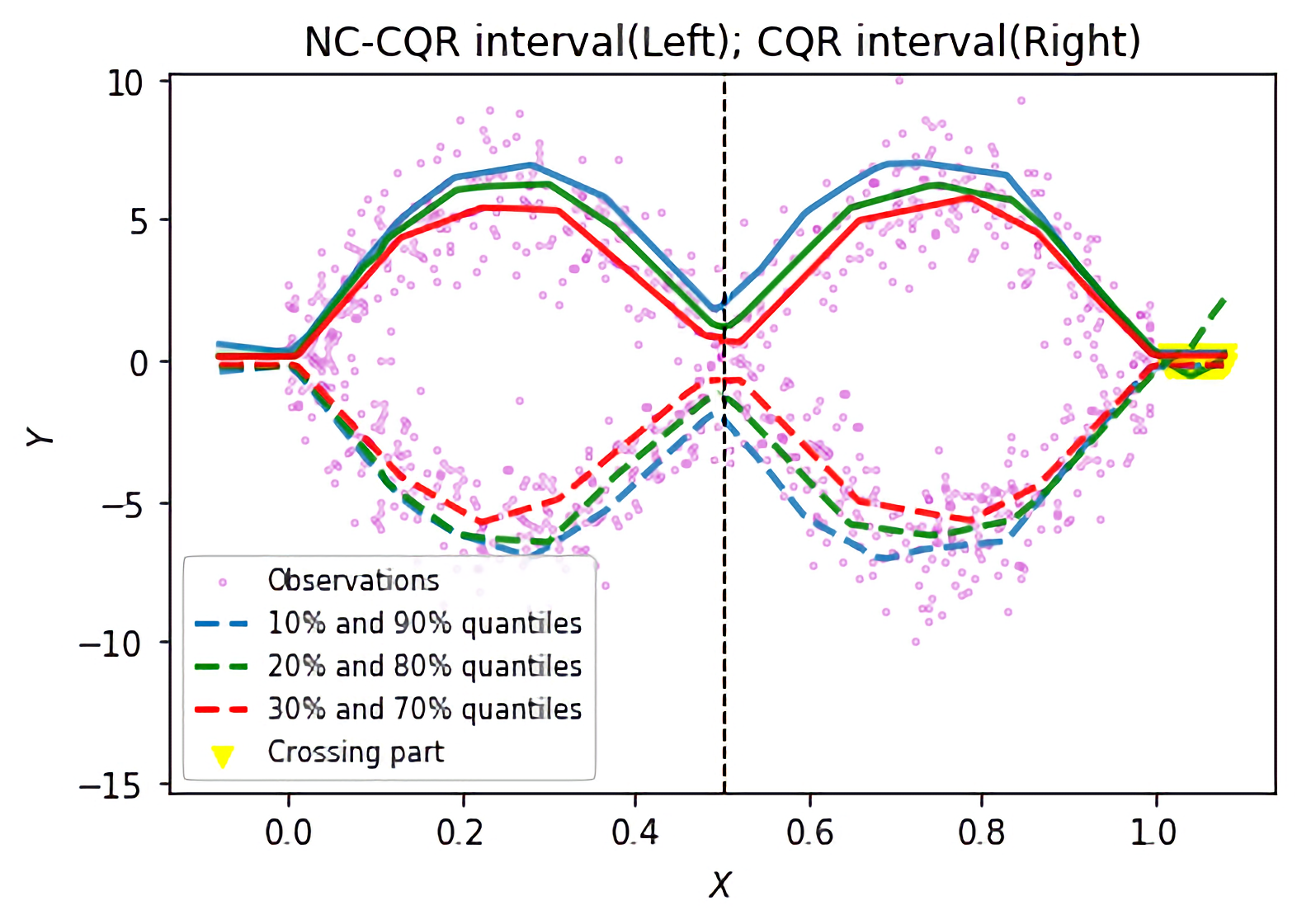
Throughout the paper, we choose the function class ${\mathcal{F}}$ to be a function class of feedforward neural networks. We note that other approximation classes can also be used. However, an important advantage of neural network functions is that they are effective in approximating smooth functions in $\mathbb{R}^{d}$, see, for example, Jiao et al., (2021) and the references therein. A detailed description of neural network functions will be given in Section 2.2. Figure 1 previews non-crossing curve estimation via a toy example, which shows the comparison between the proposed method in (7) (with penalty) and the deep quantile estimation studied in Shen et al., (2021) (without penalty); see Section B.1.2 in Appendix for more details.

Figure 1: A toy example shows that NC-CQR can avoid quantile crossing. The quantile curves on the left panel are estimated by NC-CQR, and those on the right are estimated by the deep quantile regressionShen et al., (2021). The yellow color indicates quantile crossing.

Remark 2.1

The rectified linear unit (ReLU) function $\sigma(x)=\max(0,x)$ is a piecewise-linear function. An important advantage of the ReLU penalty $\max\{f_{1}-f_{2},0\}$ is that it is convex with respect to $f_{1}$ and $f_{2}$, thus the loss function in (6) is also convex with respect to $f_{1}$ and $f_{2}$.

Remark 2.2

The tuning parameter $\lambda$ controls the amount of penalty on crossing quantile curves. As shown in Section 4, a bigger $\lambda$ leads to a larger estimation bias. Therefore, there is a trade-off between the crossing and the accuracy of prediction intervals. Both can be achieved with proper choice of $\lambda$. In the appendix, we propose a cross-validation method to select $\lambda$.

Remark 2.3

Bondell et al., (2010) proposed a non-crossing nonparametric quantile regression using smoothing splines with non-crossing constraints. For two given quantile levels $0<\tau_{1}<\tau_{2}<1$, they proposed to estimate the quantile curves $f_{\tau_{1}}$ and $f_{\tau_{2}}$ by minimizing the following constrained loss function

$$\min_{f_{1},f_{2}} \sum_{t=1}^{2}\sum_{i=1}^{n}\rho_{\tau_{t}}\left(Y_{i}-f_{{t}}\left(X_{i}\right)\right)+\sum_{t=1}^{2}\lambda_{\tau_{t}}V^{\ast}\left(f_{{t}}^{\prime}\right)$$

$$\quad\text{ subject to }f_{{2}}(x)\geq f_{{1}}(x)\ \text{ for all }x\in{\mathcal{X}},$$ (8)

where $f^{\prime}$ denotes the derivative of a function $f$, and $V^{\ast}(f^{\prime})=\int_{0}^{1}|f^{\prime\prime}(t)|dt$ is the total variation penalty to guarantee smoothness. Such a spline-based method works well in the one-dimensional setting, however, it is difficult to apply this approach to multi-dimensional problems.

2.2 ReLU Feedforward neural networks

For the estimation of conditional quantile functions, we choose the function class $\mathcal{F}$ in (7) to be $\mathcal{F}_{\mathcal{D},\mathcal{W},U,\mathcal{S},\mathcal{B}}$, a class of feedforward neural networks $f_{\phi}:$ $\mathbb{R}^{d}\rightarrow\mathbb{R}$ with parameter $\phi$, depth $\mathcal{D}$, width $\mathcal{W}$, size $\mathcal{S}$, number of neurons $\mathcal{U}$ and $f_{\phi}$ satisfying $\left\|f_{\phi}\right\|_{\infty}\leq\mathcal{B}$ for some positive constant ${\mathcal{B}}$, where $\|f\|_{\infty}$ is the supreme norm of a function $f:\mathbb{R}^{d}\rightarrow\mathbb{R}$. Note that the network parameters may depend on the sample size $n$, but this dependence is omitted for notational simplicity. Such a network $f_{\phi}$ has $\mathcal{D}$ hidden layers and $(\mathcal{D}+2)$ layers in total. We use a $(\mathcal{D}+2)$ vector $(w_{0},w_{1},\ldots,w_{\mathcal{D}},w_{\mathcal{D}+1})$ to describe the width of each layer; particularly in nonparametric regression problems, $w_{0}=d$ is the dimension of the input and $w_{\mathcal{D}+1}=1$ is the dimension of the response. The width $\mathcal{W}$ is defined as the maximum width of hidden layers, i.e., $\mathcal{W}=\max\left\{w_{1},\ldots,w_{\mathcal{D}}\right\};$ the size $\mathcal{S}$ is defined as the total number of parameters in the network $f_{\phi}$, i.e., $\mathcal{S}=\sum_{i=0}^{\mathcal{D}}w_{i+1}(w_{i}+1);$ the number of neurons $\mathcal{U}$ is defined as the number of computational units in hidden layers, i.e., $\mathcal{U}=\sum_{i=1}^{\mathcal{D}}w_{i}.$ For an MLP $\mathcal{F}_{\mathcal{D},\mathcal{U},\mathcal{W},\mathcal{S},\mathcal{B}}$, its size $\mathcal{S}$ satisfies $\max\{\mathcal{W},\mathcal{D}\}\leq\mathcal{S}\leq\mathcal{W}(\mathcal{D}+1)+\left(\mathcal{W}^{2}+\mathcal{W}\right)(\mathcal{D}-1)+\mathcal{W}+1.$

From now on, we write $\mathcal{F}_{\mathcal{D},\mathcal{W},U,\mathcal{S},\mathcal{B}}$ as ${\mathcal{F}}_{\phi}$ for short. Then, at the population level, the non-crossing nonparametric quantile estimation is to find a pair of measurable functions $(f_{\phi 1}^{\ast},f_{\phi 2}^{\ast})\in{\mathcal{F}}_{\phi}$ satisfying

$$(f_{\phi 1}^{\ast},f_{\phi 2}^{\ast}):=\arg\min_{f_{1},f_{2}\in{\mathcal{F}}_{\phi}}{\mathcal{R}}^{\tau_{1},\tau_{2}}(f_{1},f_{2}).$$ (9)

3 Non-crossing quantile regression for conformal prediction

Now suppose we have a new observation $X_{n+1}$. We are interested in predicting the corresponding unknown value of $Y_{n+1}$. Our goal is to construct a distribution-free prediction interval $C\left(X_{n+1}\right)\subseteq\mathbb{R}$ with a coverage probability satisfying

$$\mathbb{P}\left\{Y_{n+1}\in C\left(X_{n+1}\right)\right\}\geq 1-\alpha$$ (10)

for any joint distribution ${\mathbb{P}}_{XY}$ and any sample size $n$, where $0<\alpha<1$ is often called a miscoverage rate. We refer to such a coverage stated in (10) as marginal coverage.

First, we define an oracle prediction band based on the conditional quantile functions. For a pre-specified miscoverage rate $\alpha$, we consider the lower and upper quantiles levels such as $\tau_{1}=\alpha/2$ and $\tau_{2}=1-\alpha/2$. Then, a conditional prediction interval for $Y$ given $X=x$ with a nominal miscoverage rate $\alpha$ is

$$C^{\ast}(x)=[f_{\tau_{1}}(x),f_{\tau_{2}}(x)],$$ (11)

where $f_{\tau_{1}}$ and $f_{\tau_{2}}$ are the conditional quantile functions defined in (1) for quantile levels $\tau_{1}$ and $\tau_{2},$ respectively. Such a prediction interval with true quantile functions is ideal but cannot be constructed, only a corresponding empirical version can be estimated based on data in practice.

Next, we use the split conformal method Vovk et al., (2005) for constructing non-crossing conformal intervals. We split the observations $\left\{\left(X_{i},Y_{i}\right)\right\}_{i=1}^{n}$ into two disjoint sets: a training set $\mathcal{I}_{1}$ and a calibration set $\mathcal{I}_{2}$. Non-crossing deep neural estimators of $f_{\tau_{1}}$ and $f_{\tau_{2}}$ based on the training set $\mathcal{I}_{1}$ are given by

$$(\hat{f}_{1},\hat{f}_{2})\in \arg\min_{f_{1},f_{2}\in{\mathcal{F}}_{\phi}}\mathcal{R}^{\tau_{1},\tau_{2}}_{\mathcal{I}_{1}}(f_{1},f_{2}),$$ (12)

where

$$\mathcal{R}^{\tau_{1},\tau_{2}}_{\mathcal{I}_{1}}(f_{1},f_{2})\coloneqq\sum_{i\in\mathcal{I}_{1}}\big{[}\rho_{\tau_{1}}\left\{y_{i}-f_{{1}}\left(x_{i}\right)\right\}+\rho_{\tau_{2}}\left\{y_{i}-f_{{2}}\left(x_{i}\right)\right\}\big{]}+\lambda\sum_{i={\mathcal{I}}_{1}}V(f_{1},f_{2};x_{i})$$

and $\lambda\geq 0$ is a tuning parameter. A key step is to compute the conformity score based on the calibration set $\mathcal{I}_{2}$ Romano et al., (2019), which is defined as

$$\mathcal{E}_{i}:=\max\left\{\hat{f}_{{1}}\left(X_{i}\right)-Y_{i},Y_{i}-\hat{f}_{2}\left(X_{i}\right)\right\},\ \ \ i\in\mathcal{I}_{2}.$$ (13)

Let $\mathcal{E}=\{\mathcal{E}_{i}\}_{i\in{\mathcal{I}}_{2}}$. The conformity scores in $\mathcal{E}$ quantify the errors incurred by the plug-in prediction interval $\left[\hat{f}_{1}(x),\hat{f}_{2}(x)\right]$ evaluated on the calibration set ${\mathcal{I}}_{2}$, and can account for undercoverage and overcoverage.

Finally, for a new input data point $X_{n+1}$ and $\alpha\in(0,0.5)$, the $100(1-\alpha)\%$ prediction interval for $Y_{n+1}$ is defined as

$$\hat{C}\left(X_{n+1}\right)=\left[\hat{f}_{{1}}\left(X_{n+1}\right)-Q_{1-\alpha}\left(\mathcal{E},\mathcal{I}_{2}\right),\hat{f}_{2}\left(X_{n+1}\right)+Q_{1-\alpha}\left(\mathcal{E},\mathcal{I}_{2}\right)\right],$$ (14)

where $Q_{1-\alpha}\left(\mathcal{E},\mathcal{I}_{2}\right)$ is the $(1-\alpha)\left(1+1/\left|\mathcal{I}_{2}\right|\right)$-th empirical quantile of $\left\{\mathcal{E}_{i}:i\in\mathcal{I}_{2}\right\}$, namely, the $\lceil(|{\mathcal{I}}_{2}|+1)(1+\alpha)\rceil$-th smallest value in $\left\{\mathcal{E}_{i}:i\in\mathcal{I}_{2}\right\}$, and $\lceil a\rceil$ denotes the smallest integer no less than $a$. Here, $|\mathcal{I}|$ is the cardinality of a set $\mathcal{I}$. The empirical quantile $Q_{1-\alpha}\left(\mathcal{E},\mathcal{I}_{2}\right)$ is a data-driven quantity, which conformalizes the plug-in prediction interval.

In contrast to the conformalized quantile regression procedure in Romano et al., (2019), our method produces conformal prediction intervals that avoid the quantile crossing problem. We refer to the proposed non-crossing conformalized quantile regression as NC-CQR, and the corresponding conformal interval (14) as NC-CQR interval.

Remark 3.1

The usual linear quantile regression (QR) model assumes that, for a given $\tau\in(0,1)$,

$$Q_{\tau}(Y|X=x)=a_{\tau}+b_{\tau}^{\top}x,$$ (15)

where $a_{\tau}\in\mathbb{R}$ and $b_{\tau}\in\mathbb{R}^{d}$ are the intercept and slope parameters. Following Romano et al., (2019), a conformal interval based on linear quantile regression can be constructed. Specifically, by splitting the observations $\left\{\left(X_{i},Y_{i}\right)\right\}_{i=1}^{n}$ into two disjoint subsets: a training set $\mathcal{I}_{1}$ and a calibration set $\mathcal{I}_{2}$, we can fit model (15) on the training set ${\mathcal{I}}_{1}$ and obtain the estimators for $a_{\tau}$ and $b_{\tau}$ for a given $\tau\in(0,1)$, denoted by $(\hat{a}_{\tau},\hat{b}_{\tau})$. Under model (15), the conformal interval with miscoverage rate $\alpha$ is given by

$$\hat{C}_{\rm qr}(x)=[\hat{f}_{\rm lo}(x)-\hat{Q}_{\rm qr},\ \ \hat{f}_{\rm hi}(x)+\hat{Q}_{\rm qr}],$$ (16)

where $\hat{f}_{\rm lo}(x):=x^{\top}\hat{b}_{\tau_{\rm lo}}+\hat{a}_{\tau_{\rm lo}}$, $\hat{f}_{\rm hi}(x):=x^{\top}\hat{b}_{\tau_{\rm hi}}+\hat{a}_{\tau_{\rm hi}}$ with $\tau_{\rm lo}=\alpha/2$ and $\tau_{\rm hi}=1-\alpha/2$, and $\hat{Q}_{\rm qr}$ is the $\lceil(|{\mathcal{I}}_{2}|+1)(1+\alpha)\rceil$-th smallest value among the conformity scores $\mathcal{E}_{i}^{\rm qr}=\max\{\hat{f}_{\rm lo}(x)-y_{i},y_{i}-\hat{f}_{\rm hi}(x_{i})\},i\in\mathcal{I}_{2}$.

We summarize the implementation of NC-CQR interval construction in the following algorithm.

Algorithm Computation of non-crossing conformalized prediction intervals

Input: Observations $S=\{(X_{i},Y_{i})\}_{i=1}^{n}$ and miscoverage level $\alpha\in(0,0.5).$

Output: $C\left(x\right)=\left[\hat{f}_{{1}}\left(x\right)-Q_{1-\alpha}\left(\mathcal{E},\mathcal{I}_{2}\right),\hat{f}_{2}\left(x\right)+Q_{1-\alpha}\left(\mathcal{E},\mathcal{I}_{2}\right)\right].$

Steps:

1. Split $S$ into a training set $S_{1}=\{(X_{i},Y_{i})\}_{i\in{\mathcal{I}}_{1}}$ and a calibration set $S_{2}=\{(X_{i},Y_{i})\}_{i\in{\mathcal{I}}_{2}}$.
   

2. Fit $S_{1}$ to (12) to obtain $(\hat{f}_{1},\hat{f}_{2})$ for $\tau_{1}=1-\alpha/2$ and $\tau_{2}=\alpha/2$.
   

3. Compute the conformity score $\mathcal{E}_{i}:=\max\{\hat{f}_{{1}}\left(X_{i}\right)-Y_{i},Y_{i}-\hat{f}_{2}\left(X_{i}\right)\}$, $i\in{\mathcal{I}}_{2}.$
   

4. Find $Q_{1-\alpha}\left(\mathcal{E},\mathcal{I}_{2}\right)$, the $\lceil(|{\mathcal{I}}_{2}|+1)(1+\alpha)\rceil$-th smallest value of $\mathcal{E}_{i},i\in{\mathcal{I}}_{2}.$
      5. Compute the prediction band $C\left(x\right)$ according to (14).

4 Theoretical properties

In this section, we study the theoretical properties of the proposed NC-CQR method. We evaluate NC-CQR using the following two criteria:

• Validity: Under proper conditions, a conformal prediction interval $\hat{C}$ satisfies that

  $$\mathbb{P}(Y_{n+1}\in\hat{C}(X_{n+1}))\geq 1-\alpha.$$ (17)

• Accuracy: If the validity requirement (17) is satisfied, a conformal prediction interval should be as narrow as possible.

The validity requirement (17) is evaluated based on the finite-sample marginal coverage in (10), which holds in the sense of averaging over all possible test values of $X_{n+1}$. The accuracy of a prediction interval is usually measured by the discrepancy defined in (19) between the lengths of the prediction interval and the oracle one.

We assume that the target conditional quantile function $f_{\tau}$ defined in (1) is a $\beta$-Hölder smooth function with $\beta>0$ as stated in condition (C3) below. Let $\beta=s+r>0$, $r\in(0,1]$ and $s=\lfloor\beta\rfloor\in\mathbb{N}_{0}$, where $\lfloor\beta\rfloor$ denotes the largest integer strictly smaller than $\beta$ and $\mathbb{N}_{0}$ denotes the set of non-negative integers. For a finite constant $B_{0}>0$, the Hölder class of functions $f:[0,1]^{d}\to\mathbb{R}$ is defined as

$$\mathcal{H}^{\beta}([0,1]^{d},B_{0})=\Big{\{}f:\max_{\|\alpha\|_{1}\leq s}\|\partial^{\alpha}f\|_{\infty}\leq B_{0},\max_{\|\alpha\|_{1}=s}\sup_{x\not=y}\frac{|\partial^{\alpha}{f(y)}-\partial^{\alpha}f(x)|}{\|x-y\|_{2}^{r}}\leq B_{0}\Big{\}},$$ (18)

where $\partial^{\alpha}=\partial^{\alpha_{1}}\cdots\partial^{\alpha_{d}}$ with $\alpha=(\alpha_{1},\ldots,\alpha_{d})^{\top}\in\mathbb{N}_{0}^{d}$ and $\|\alpha\|_{1}=\sum_{i=1}^{d}\alpha_{i}$. We assume the following conditions.

• (C1) The observations $\{(X_{i},Y_{i})\}_{i=1}^{n}$ are i.i.d. copies of $(X,Y)$.

• (C2) (i) The support of the predictor vector $\mathcal{X}$ is a bounded compact set in $\mathbb{R}^{d}$, and without loss of generality we let $\mathcal{X}=[0,1]^{d};$ (ii) Let $\nu$ be the probability measure of $X$. The probability measure $\nu$ is absolutely continuous with respect to the Lebesgue measure.

• (C3) For any fixed $\tau\in(0,1)$, the target conditional quantile function $f_{\tau}$ defined in (1) is a Hölder smooth function of order $\beta$ and a finite constant $B_{0}$.

• (C4) There exist constants $\gamma>0$ and $\kappa_{\tau}>0$ such that for any $|\delta|\leq\gamma$ and any $\tau\in(0,1)$,

  $$\left|F\left(f_{\tau}(x)+\delta\mid x\right)-F\left(f_{\tau}(x)\mid x\right)\right|\geq\kappa_{\tau}|\delta|$$

  for all $x\in\mathcal{X}$ up to a $\nu$-negligible set, where $F(\cdot\mid x)$ is the conditional cumulative distribution function of $Y$ given $X=x$.

Condition (C1) is a basic assumption in conformal inference. The boundedness support assumption in Condition (C2) is made for technical convenience in the proof for deep neural estimation. Condition (C3) is a regular smoothness assumption on the target regression functions so that whose approximation result using deep neural networks can be obtained. Condition (C4) is imposed for self-calibration of the resulting neural estimator.

Theorem 4.1

Under Condition (C1), for a new i.i.d pair $(X_{n+1},Y_{n+1})$, the proposed NC-CQR interval $\hat{C}(X_{n+1})$ satisfies ${{\mathbb{P}}}(Y_{n+1}\in\hat{C}(X_{n+1}))\geq 1-\alpha.$

Theorem 4.1 shows that the proposed NC-CQR interval enjoys a rigorous coverage guarantee. The proof of this theorem is given in the Appendix.

We now quantify the accuracy of the prediction interval in terms of the difference between the NC-CQR interval $\hat{C}(X)$ and the oracle $C^{\ast}(X)$ in (11) on the support of ${\mathcal{X}}.$ Let $\nu$ be the probability measure of $X$ defined in Condition (C2) and define $\|f-g\|_{L^{p}(\nu)}\coloneqq\{{\mathbb{E}}|f(X)-g(X)|^{p}\}^{1/p}$ for $p\geq 1$. The difference between the lengths of $\hat{C}(X)$ and $C^{\ast}(X)$ is given by

$$\Delta_{\mathcal{X}}(C^{\ast},\hat{C})\coloneqq \mathbb{E}\Big{[}\|(\hat{f}_{2}+Q_{1-\alpha}\left(\mathcal{E},\mathcal{I}_{2}\right))-(\hat{f}_{1}-Q_{1-\alpha}\left(\mathcal{E},\mathcal{I}_{2}\right))\|_{L^{2}(\nu)}-\|f_{\tau_{2}}-f_{\tau_{1}}\|_{L^{2}(\nu)}\Big{]}.$$ (19)

By the triangle inequality, we have $\Delta_{\mathcal{X}}(C^{\ast},\hat{C})\leq I_{1}+I_{2}+I_{3},$ where

$$I_{1}:=\mathbb{E}\|\hat{f}_{2}-f_{\tau_{2}}\|_{L^{2}(\nu)},I_{2}:=\mathbb{E}\|\hat{f}_{1}-f_{\tau_{1}}\|_{L^{2}(\nu)}\text{ and }I_{3}:=2\mathbb{E}\|Q_{1-\alpha}\left(\mathcal{E},\mathcal{I}_{2}\right)\|_{L^{2}(\nu)}.$$

To bound $I_{1}$ and $I_{2}$, we need to bound the error $\|\hat{f}-f_{\tau}\|_{L^{2}(\nu)}.$ To this end, we first derive bounds for the the excess risk of $(\hat{f}_{1},\hat{f}_{2})$ defined as $\mathbb{E}\{\mathcal{R}^{\tau_{1},\tau_{2}}(\hat{f}_{1},\hat{f}_{2})-\mathcal{R}^{\tau_{1},\tau_{2}}\left({f}_{\tau_{1}},{f}_{\tau_{2}}\right)\},$ where $\mathcal{R}^{\tau_{1},\tau_{2}}$ is defined in (5). Without loss of generality, we assume that $|{\mathcal{I}}_{1}|=\lceil n/2\rceil$ and $|{\mathcal{I}}_{2}|=\lfloor n/2\rfloor$, where $\lceil a\rceil$ denotes the smallest integer no less than $a$ and $\lfloor a\rfloor$ denotes the largest integer no greater than $a$.

Theorem 4.2

Letting $N=1$ and $L=\lfloor n^{d/2(d+\beta)}\rfloor$, then the width, depth and size of the neural network satisfy

$$\mathcal{W} =114(\lfloor\beta\rfloor+1)^{2}d^{\lfloor\beta\rfloor+1},\ \mathcal{D}=21(\lfloor\beta\rfloor+1)^{2}\left\lceil n^{d/2(d+\beta)}\log_{2}\left(8n^{d/2(d+\beta)}\right)\right\rceil,$$

$$\mathcal{S} =O\left((\lfloor\beta\rfloor+1)^{6}d^{2\lfloor\beta\rfloor+2}\left\lceil n^{d/2(d+\beta)}(\log n)\right\rceil\right).$$

Suppose that Conditions (C1)-(C3) hold. If $\lambda=\log n$, the non-asymptotic error bound of the excess risk satisfies

$$\mathbb{E}\left\{\mathcal{R}^{\tau_{1},\tau_{2}}\left(\hat{f}_{1},\hat{f}_{2}\right)-\mathcal{R}^{\tau_{1},\tau_{2}}\left({f}_{\tau_{1}},{f}_{\tau_{2}}\right)\right\}\leq c_{1}(\lfloor\beta\rfloor+1)^{8}d^{2(\lfloor\beta\rfloor+1)}(\log n)^{5}n^{-\frac{\beta}{d+\beta}},$$

where $c_{1}>0$ is a universal constant independent of $n,d,\tau,{B},\mathcal{S},\mathcal{W}$ and $\mathcal{D}$ and $a\vee b:=\max\{a,b\}$.

The convergence rate of the excess risk is $n^{-\beta/(d+\beta)}$ up to a logarithmic factor. The next theorem gives an upper bound for the accuracy of the proposed prediction interval defined in (19).

Theorem 4.3

(Non-asymptotic upper bound for prediction accuracy) Suppose that Conditions (C1)-(C4) hold. Let $\mathcal{F}_{\phi}=\mathcal{F}_{\mathcal{D},\mathcal{W},\mathcal{U},\mathcal{S},\mathcal{B}}$ be a class of ReLU activated feedforward neural networks with width, depth specified as in Theorem 4.2 and let $(\hat{f}_{1},\hat{f}_{2})\in\arg\min_{f_{1},f_{2}\in\mathcal{F}_{\phi}}R_{n}^{\tau_{1},\tau_{2}}(f_{1},f_{2})$ be the empirical risk minimizer over $\mathcal{F}_{\phi}$. Then, there exists a constant $N>0$, for $n>N$,

$$\Delta_{\mathcal{X}}(C^{\ast},\hat{C})\leq c(\lfloor\beta\rfloor+1)^{8}d^{2(\lfloor\beta\rfloor+1)}(\log n)^{4}n^{-\beta/(d+\beta)},$$

where $c>0$ is a constant independent of $n,d,\tau,{B},\mathcal{S},\mathcal{W}$ and $\mathcal{D}$.

Theorem 4.3 gives an upper bound for the difference between the lengths of our proposed prediction interval and the oracle interval. With properly-selected neural network parameters, the oracle band can be consistently estimated by the NC-CQR band.

Finally, we consider the conformal interval based on linear quantile regression defined in (16).

Corollary 4.1

Suppose that at least one of $f_{\tau_{1}}$ and $f_{\tau_{2}}$ is a non-linear function on a subset of $\mathcal{X}$ with non-zero measure. Then for any sample size $n$, the accuracy of the conformal band $\hat{C}_{\rm qr}$ defined in (16) is strictly worse than that of the oracle conformal band $C^{*}$, i.e., there exists an $\epsilon>0$ such that $\Delta_{\mathcal{X}}(C^{\ast},\hat{C}_{\rm qr})>\epsilon.$

According to Corollary 4.1, a conformal interval based on the linear quantile regression will not reach the oracle accuracy in the presence of nonlinearity.

5 Numerical studies

5.1 Synthetic data

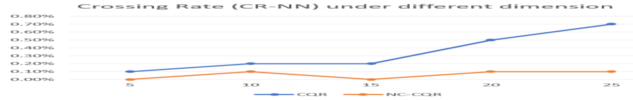
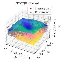
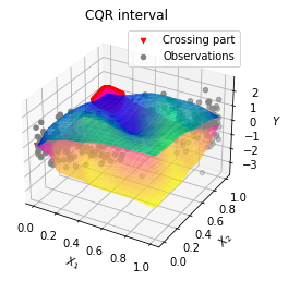
We first simulate a synthetic dataset with a $d$-dimensional feature $X$ and a continuous response $Y$ from the distributions defined in Section B.1.3. Our method is applied to $5,000$ independent observations from this distribution, using $2,000$ of them to train the deep quantile regression estimators and $2,000$ of them for calibration. The remaining data is for testing. We consider different dimensions $d=5,10,15,20,25$ to investigate how the dimensionality of the input affects the overall performance under multivariate input settings. The result is shown in Figure 2. In Figure 2(c), when dimension increases, NC-CQR method performs better than CQR in terms of smaller crossing rate. It shows that the NC-CQR method can mitigate the crossing problem in quantile regression. We also give a 3D visualization of the conformal intervals of our proposed NC-CQR estimation and that of the CQR method when $d=2$ in Figure 2. One can see from Figure 2(a) that the conformal interval by our proposed NC-CQR method does not have any crossing, while in Figure 2(b), the red region indicates that the lower bound is larger than the upper bound of the interval. More details of the results are given in Section B.1.3.

(a) The crossing rates of two methods as dimension increases.

(b) The non-crossing quantile interval.

(c) The quantile interval without non-crossing penalty.

Figure 2: The comparison between the proposed interval estimation with penalty and interval estimation without penalty. The blue surface is the estimated $80\%$-th upper quantile surface and the yellow surface is the $20\%$-th lower quantile surface. Red color indicates quantile crossing.

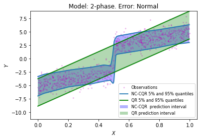
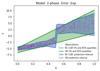
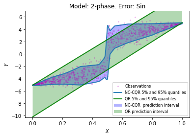
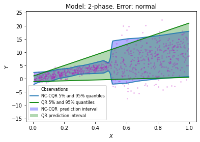
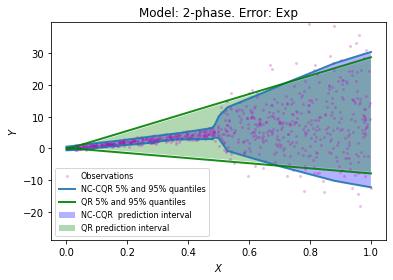
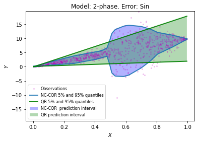
Our next synthetic example illustrates the adaptive property of the proposed NC-CQR prediction interval. We consider the following model with a discontinuous regression function:

$$Y=5X\mathbbm{1}(X\leq 0.5)+5(X-1)\mathbbm{1}(X>0.5)+\varepsilon.$$ (20)

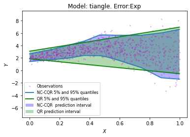
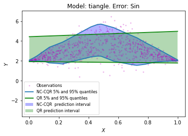
A 90% NC-CQR interval is shown in color blue. The green lines represent a 90% conformal prediction intervals based on the standard linear quantile regression. As can be seen from the plots, the NC-CQR intervals automatically adapt to the shape of the regression function and the heteroscedasticity of the model error. Additional examples demonstrating the advantages of NC-CQR prediction intervals are given in the Appendix.

Figure 3: Prediction intervals based on NC-CQR and linear QR for model (20)

5.2 Real data examples

We compute the NC-CQR prediction intervals for the following datasets: bike sharing, house price and the air foil data sets. To examine the performance of the ReLU penalty, we compare the NC-CQR with CQR. We compute the conformal prediction intervals based on these two methods using the same deep quantile regression estimator. Their performances are evaluated as in Section 5.1. We subsample $40\%$ of data for training, $40\%$ for calibration, and the remaining data is used for testing. All features are standardized to have 0 mean and unit variance. The nominal coverage rate is set to be $80\%$. Figure S5 shows that the proposed NC-CQR method can mitigate the crossing problem encountered in the CQR estimation. Additional details of the result are given in Section B.2 in the Appendix.

(a) CQR interval

(b) NC-CQR interval

Figure 4: The performance of NC-CQR and CQR on several real data sets based a deep nonparametric quantile regression model. Since the input are multidimensional, we sorted the data by the value of responses and depict them along with the corresponding estimated interval in a 2D plot.

6 Concluding remarks

We have proposed NC-CQR, a penalized deep quantile regression method which avoids the quantile crossing problem via a ReLU penalty. We have derived non-asymptotic upper bounds for the excess risk of the non-crossing empirical risk minimizers. Our error bounds achieve optimal minimax rate of convergence, the with the prefactor of the error bounds depending polynomially on the dimension of the predictor, instead of exponentially. The proposed ReLU penalty for monotonic constraints is applicable to problems with different loss functions. It is applicable to other nonparametric estimation method, including smoothing splines, kernel method and neural network. Therefore, the proposed ReLU penalty method may be of independent interest. Based on the estimated non-crossing conditional quantile curves, we construct conformal prediction intervals that are fully adaptive to heterogeneity. We have also provided conditions under which the proposed NC-CQR conformal prediction bands are valid with the correct coverage probability and achieve optimal accuracy in terms of the width of the prediction band.

A main limitation of the proposed method and the theoretical properties is that they rely on the i.i.d. assumption for the data. There are applications where observations are not independent (e.g., time series data) and there may be distribution shift. It would be interesting to extend the proposed method to deal with such non-i.i.d. settings and establish the corresponding theoretical properties.

Appendix A Appendix: Proofs

In this appendix, we prove the theoretical results stated in Section 4. First, we prove Lemma 2.1. For convenience, we restate this lemma below.

Lemma A.1

Suppose $Z$ is a random variable with c.d.f. $F(\cdot)$. For a given $\tau\in(0,1)$, any element in $\{z:F(z)=\tau\}$ is a minimizer of the expected check loss function ${\mathbb{E}}\rho_{\tau}(Z-t)$. Moreover, the pair of the true conditional quantile functions $(f_{\tau_{1}},f_{\tau_{2}})$ is the minimizer of the loss function (5), that is,

$$(f_{\tau_{1}},f_{\tau_{2}})=\arg\min_{f_{1},f_{2}\in{\mathcal{F}}}\mathcal{R}^{\tau_{1},\tau_{2}}({f}_{{1}},{f}_{{2}}),$$

where ${\mathcal{F}}$ is a class of measurable functions that contains the true conditional quantile functions.

Proof[of Lemma A.1] First, we write

$$\min_{t}{\mathbb{E}}\rho_{\tau}(Z-t)=\min\left\{\int_{-\infty}^{t}(\tau-1)(z-t)d{F}(z)+\int_{t}^{\infty}\tau(z-t)dF(z)\right\}.$$

Taking derivative w.r.t $t$, we obtain

$$0 =(1-\tau)\int_{-\infty}^{t}d{F}(z)-\tau\int_{t}^{\infty}dF(z)$$

$$=(1-\tau)F(t)-\tau(1-F(t))=F(t)-\tau.$$

Since $F(\cdot)$ is a c.d.f., it is monotonic and thus any element of $\{z:F(z)=\tau\}$ minimizes the expected loss ${\mathbb{E}}\rho_{\tau}(Z-t)$. For functions $f_{1},f_{2}$, recall that the loss function (5) in the main context is

$$\mathcal{R}^{\tau_{1},\tau_{2}}({f}_{{1}},{f}_{{2}})={\mathbb{E}}_{Z}\left[\rho_{\tau_{1}}\left\{Y-f_{{1}}\left(X\right)\right\}+\rho_{\tau_{2}}\left\{Y-f_{{2}}\left(X\right)\right\}\right]+\lambda{\mathbb{E}}_{Z}V(f_{1},f_{2};X).$$

By the definition of $f_{\tau_{k}}$ in (1) in the main context, $f_{\tau_{k}}$ satisfies $\inf\{y:F(y|X=x)\geq\tau_{k}\}$ for $k=1,2$. Then $f_{\tau_{k}}$ minimizes the expected loss ${\mathbb{E}}\rho_{\tau_{k}}(Y-f_{k}(x))$ for $k=1,2$. Since the true quantile function $(f_{\tau_{1}},f_{\tau_{2}})$ satisfies the monotonicity requirement (2) in the main context, then ${\mathbb{E}}_{Z}V(f_{\tau_{1}},f_{\tau_{2}};X)=0$. Therefore, $(f_{\tau_{1}},f_{\tau_{2}})$ is the minimizer of the loss function (5) in the main context.

Lemma A.2

Suppose that

$$\mathbb{P}\left[\mathbb{E}_{X}\left\{\left(\hat{f}_{1}(X)-f_{\tau_{2}}(X)\right)^{2}\mid{\mathcal{I}}_{1}\right\}+\mathbb{E}_{X}\left\{\left(\hat{f}_{1}(X)-f_{\tau_{2}}(X)\right)^{2}\mid{\mathcal{I}}_{1}\right\}\leq\eta_{n}\right]\geq 1-{\xi_{n}},$$ (S21)

for some sequence $\eta_{n}$ and $\xi_{n}$ such that $\eta_{n}\to 0$ and $\xi_{n}\to 0$ when $n\to\infty$. Define

$$A_{n}:=\left\{x:\left|\hat{f}_{1}\left(x\right)-f_{\tau_{1}}\left(x\right)\right|>\eta_{n}^{1/3}\right\}\cup\left\{x:\left|\hat{f}_{2}\left(x\right)-f_{\tau_{2}}\left(x\right)\right|>\eta_{n}^{1/3}\right\}.$$

Then, under Conditions (C1)-(C4), for any $X$ independent of ${\mathcal{I}}_{1}$,

$$\mathbb{P}\left[X\in A_{n}|{\mathcal{I}}_{1}\right]\leq\eta_{n}^{1/3}+\xi_{n}.$$

Furthermore, if the calibration set ${\mathcal{I}}_{2}$ is partitioned into

$$\mathcal{I}_{2,a}:=\left\{i\in\{n+1,\ldots,2n\}:X_{i}\in A_{n}\right\},\quad\mathcal{I}_{2,b}:=\left\{i\in\{n+1,\ldots,2n\}:X_{i}\in A_{n}^{\mathrm{c}}\right\},$$

then for any constant $c>0$, we have

$$\mathbb{P}\left[\left|\mathcal{I}_{2,a}\right|\geq n\left(\eta_{n}^{1/3}+\xi_{n}\right)+c\sqrt{n\log n}\right]\leq n^{-2c^{2}}.$$

Proof[of Lemma A.2] By Markov inequality, we have

$$\mathbb{P}\left[X\in A_{n}\mid{\mathcal{I}}_{1}\right]$$

$$= \mathbb{P}\left[\left|\hat{f}_{1}\left(x\right)-f_{\tau_{1}}\left(x\right)\right|>\eta_{n}^{1/3},\left|\hat{f}_{2}\left(x\right)-f_{\tau_{2}}\left(x\right)\right|>\eta_{n}^{1/3}\mid{\mathcal{I}}_{1}\right]$$

$$\leq \mathbb{P}\left[\left|\hat{f}_{1}\left(x\right)-f_{\tau_{1}}\left(x\right)\right|>\eta_{n}^{1/3}\mid{\mathcal{I}}_{1}\right]+\mathbb{P}\left[\left|\hat{f}_{2}\left(x\right)-f_{\tau_{2}}\left(x\right)\right|>\eta_{n}^{1/3}\mid{\mathcal{I}}_{1}\right]$$

$$\leq \eta_{n}^{-2/3}{E}_{X}\left[\left(\hat{f}_{1}(X)-{f}_{\tau_{1}}(X)\right)^{2}\mid{\mathcal{I}}_{1}\right]+\eta_{n}^{-2/3}{E}_{X}\left[\left(\hat{f}_{2}(X)-{f}_{\tau_{2}}(X)\right)^{2}\mid{\mathcal{I}}_{1}\right]$$

$$\leq \eta_{n}^{1/3}+\xi_{n}.$$

When the calibration set ${\mathcal{I}}_{2}$ is partitioned into

$$\mathcal{I}_{2,a}:=\left\{i\in{\mathcal{I}}_{2}:X_{i}\in A_{n}\right\},\quad\mathcal{I}_{2,b}:=\left\{i\in{\mathcal{I}}_{2}:X_{i}\in A_{n}^{\mathrm{c}}\right\},$$

it follows from Hoeffding’s inequality that, for any $t>0$,

$$\mathbb{P}\left[\left|\mathcal{I}_{2,a}\right|\geq n\left(\eta_{n}^{1/3}+\xi_{n}\right)+t\right]$$

$$\leq \mathbb{P}\left[\left|\mathcal{I}_{2,a}\right|\geq n\mathbb{P}\left[X\in A_{n}\right]+t\right]$$

$$\leq \mathbb{P}\left[\frac{1}{n}\sum_{i=n+1}^{2n}\mathbbm{1}\left[X_{i}\in A_{n}\right]\geq\mathbb{P}\left[X_{i}\in A_{n}\right]+\frac{t}{n}\right]$$

$$\leq \mathbb{P}\left[\frac{1}{n}\sum_{i=n+1}^{2n}\mathbbm{1}\left[X_{i}\in A_{n}\right]-\mathbb{P}\left[X_{i}\in A_{n}\right]\geq\frac{t}{n}\right]$$

$$\leq \exp\left(-\frac{2t^{2}}{n}\right).$$

Letting $t=c\sqrt{n\log n}$, the proof of the second inequality in Lemma (A.2) is completed.

Proof[of Theorem 4.1] The proof of Theorem 4.1 is similar to that of Theorem 1 in Romano et al., (2019). Let $\mathcal{E}_{n+1}$ be the conformity score

$$\mathcal{E}_{n+1}:=\max\left\{\hat{f}_{{1}}\left(X_{n+1}\right)-Y_{n+1},Y_{n+1}-\hat{f}_{{2}}\left(X_{n+1}\right)\right\}$$

at the test point $\left(X_{n+1},Y_{n+1}\right).$ Recall that the prediction interval

$$\hat{C}\left(X_{n+1}\right)=[\hat{f}_{{1}}\left(X_{n+1}\right)-Q_{1-\alpha}(\mathcal{E},\mathcal{I}_{2}),\hat{f}_{{2}}\left(X_{n+1}\right)+Q_{1-\alpha}(\mathcal{E},\mathcal{I}_{2})].$$

By the construction of the prediction interval, $Y_{n+1}\in\hat{C}\left(X_{n+1}\right)$ if and only if $\mathcal{E}_{n+1}\leq Q_{1-\alpha}\left(\mathcal{E},\mathcal{I}_{2}\right)$, and particularly,

$$\mathbb{P}\left\{Y_{n+1}\in\hat{C}\left(X_{n+1}\right)\mid\left(X_{i},Y_{i}\right)_{i\in\mathcal{I}_{1}}\right\}$$

$$= \mathbb{P}\left\{\hat{f}_{{1}}\left(X_{n+1}\right)-Q_{1-\alpha}(\mathcal{E},\mathcal{I}_{2})\leq Y_{n+1}\leq\hat{f}_{{2}}\left(X_{n+1}\right)+Q_{1-\alpha}(\mathcal{E},\mathcal{I}_{2})\mid\left(X_{i},Y_{i}\right)_{i\in\mathcal{I}_{1}}\right\}$$

$$= \mathbb{P}\left\{\hat{f}_{{1}}\left(X_{n+1}\right)-Y_{n+1}\leq Q_{1-\alpha}(\mathcal{E},\mathcal{I}_{2})\ ,\ Y_{n+1}-\hat{f}_{{2}}\left(X_{n+1}\right)\leq Q_{1-\alpha}(\mathcal{E},\mathcal{I}_{2})\mid\left(X_{i},Y_{i}\right)_{i\in\mathcal{I}_{1}}\right\}$$

$$= \mathbb{P}\left[\max\left\{\hat{f}_{{1}}\left(X_{n+1}\right)-Y_{n+1},Y_{n+1}-\hat{f}_{{2}}\left(X_{n+1}\right)\right\}\leq Q_{1-\alpha}(\mathcal{E},\mathcal{I}_{2})\mid\left(X_{i},Y_{i}\right)_{i\in\mathcal{I}_{1}}\right]$$

$$= \mathbb{P}\left\{\mathcal{E}_{n+1}\leq Q_{1-\alpha}\left(\mathcal{E},\mathcal{I}_{2}\right)\mid\left(X_{i},Y_{i}\right)_{i\in\mathcal{I}_{1}}\right\}.$$

Since the data $(X_{i},Y_{i}),i=1,\ldots,n$ are i.i.d, so are the calibration variables $\mathcal{E}_{i}$ for $i\in\mathcal{I}_{2}$ and $i=n+1$. Therefore, by Lemma 2 on inflated empirical quantiles in Romano et al., (2019), we can conclude that

$$\mathbb{P}\left\{\mathcal{E}_{n+1}\leq Q_{1-\alpha}\left(\mathcal{E},\mathcal{I}_{2}\right)\mid\left(X_{i},Y_{i}\right):i\in\mathcal{I}_{1}\right\}\geq 1-\alpha.$$

We now present a non-asymptotic upper bound for the excess risk.

Lemma A.3

(Non-asymptotic excess risk bound) Consider the $d$-variate nonparametric regression model in (1) in the paper. For any given $N,L\in\mathbb{N}^{+}$, Let $\mathcal{F}_{\phi}=\mathcal{F}_{\mathcal{D},\mathcal{W},\mathcal{U},\mathcal{S},\mathcal{B}}$ be a class of feedforward neural networks with ReLU activation function with width $\mathcal{W}$ and depth $\mathcal{D}$ specified by

$$\mathcal{W}=38(\lfloor\beta\rfloor+1)^{2}d^{\lfloor\beta\rfloor+1}N\lceil\log_{2}(8N)\rceil,\ \mathcal{D} =21(\lfloor\beta\rfloor+1)^{2}L\lceil\log_{2}(8L)\rceil.$$

Assume that Conditions (C1)-(C3) hold with $B_{0}\leq\mathcal{B}$. For any given $0<\tau_{1}<\tau_{2}<1$, let $f_{\tau_{1}}$ and $f_{\tau_{2}}$ denote the corresponding conditional quantile functions and let

$$(\hat{f}_{1},\hat{f}_{2})\in\arg\min_{f_{1},f_{2}\in\mathcal{F}_{\phi}}R_{n}^{\tau_{1},\tau_{2}}(f_{1},f_{2})$$

be the empirical risk minimizer (ERM) over $\mathcal{F}_{\phi}$, then

$$\mathbb{E}\left\{\mathcal{R}^{\tau_{1},\tau_{2}}\left(\hat{f}_{1},\hat{f}_{2}\right)-\mathcal{R}^{\tau_{1},\tau_{2}}\left({f}_{\tau_{1}},{f}_{\tau_{2}}\right)\right\}$$

$$\quad\leq c_{0}\frac{(1+\lambda)\mathcal{B}\log(n){\mathcal{S}}{\mathcal{D}}\log({\mathcal{S}})}{n}+72B_{0}(\lfloor\beta\rfloor+1)^{2}d^{\lfloor\beta\rfloor+(\beta\vee 1)/2}(NL)^{-2\beta/d},$$ (S22)

where $c_{0}>0$ is a universal constant independent of $n,d,\tau,{B},\mathcal{S},\mathcal{W}$ and $\mathcal{D}$, and $a\vee b:=\max(a,b).$

Lemma A.3 provides a general non-asymptotic upper bound for the excess risk. This bound clearly describes how the upper bounds of the excess risk depend on the neural network parameters. The first term of the bound (A.3) is the upper bound of the stochastic error and the second term is the upper bound of the approximation error. Notice that the stochastic error increases with $(N,L)$, while the approximation error decreases with $(N,L)$. Similar to Shen et al., (2021), we next discuss efficient designs of rectangle networks, i.e., networks with equal width for each hidden layer. It follows from the standard structure of multilayer perceptrons that the size of network ${\mathcal{S}}=O(\mathcal{W}^{2}{\mathcal{D}})$. Thus, we can select the neural network width and depth given in terms of $(N,L)$ to balance the stochastic error and approximation error, so as to achieve the optimal convergence rate.

Proof[of Lemma A.3] The sample size of the training set is $\lfloor n/2\rfloor$. Without loss of generality, we let the size of training data $l$ to be proportional to $n$, i.e., there exists a constant $c_{0}\geq 0$ such that $l=c_{0}n$. Let $S=\left\{Z_{i}=\left(X_{i},Y_{i}\right)\right\}_{i=1}^{l}$ be a random sample from the distribution of $Z=(X,Y)$ and let $S^{\prime}=\left\{Z_{i}^{\prime}=\left(X_{i}^{\prime},Y_{i}^{\prime}\right)\right\}_{i=1}^{m}$ be another random sample independent of $S$. First, for any $f_{1},f_{2}\in\mathcal{F}_{\phi}$ and $Z_{i}=(X_{i},Y_{i})$, we denote

$$g(f_{1},f_{2},X_{i})=\mathbb{E}\{m(f_{1},f_{2},Z_{i})+h(f_{1},f_{2},X_{i})\mid X_{i}\},$$

where

$$m(f_{1},f_{2},Z_{i}):= \rho_{\tau_{1}}(f_{1}(X_{i})-Y_{i})+\rho_{\tau_{2}}(f_{2}(X_{i})-Y_{i})-\rho_{\tau_{1}}(f_{\tau_{1}}(X_{i})-Y_{i})$$

$$-\rho_{\tau_{2}}(f_{\tau_{2}}(X_{i})-Y_{i})$$

$$h(f_{1},f_{2},X_{i}):= \lambda[\max\{f_{1}(X_{i})-f_{2}(X_{i}),0\}-\max\{f_{\tau_{1}}(X_{i})-f_{\tau_{2}}(X_{i}),0\}].$$

Note that for any $\tau_{1}<\tau_{2}$, $f_{\tau_{1}}(x)-f_{\tau_{2}}(x)\leq 0\forall x$ and

$$|h(f_{1},f_{2},X_{i})| \leq 4\lambda\mathcal{B}$$

$$|m(f_{1},f_{2},Z_{i})| \leq 4\mathcal{B}$$

$$|g(f_{1},f_{2},X_{i})| \leq 4(1+\lambda)\mathcal{B}.$$

Then the excess risk of $(\hat{f}_{1},\hat{f}_{2})$

$$\mathcal{R}^{\tau_{1},\tau_{2}}\left(\hat{f}_{1},\hat{f}_{2}\right)-\mathcal{R}^{\tau_{1},\tau_{2}}\left({f}_{\tau_{1}},{f}_{\tau_{2}}\right)={\mathbb{E}}_{S^{\prime}}\{g(\hat{f}_{1},\hat{f}_{2},X_{i}^{\prime})\},$$

and the expected excess risk

$${\mathbb{E}}\{\mathcal{R}^{\tau_{1},\tau_{2}}\left(\hat{f}_{1},\hat{f}_{2}\right)-\mathcal{R}^{\tau_{1},\tau_{2}}\left({f}_{\tau_{1}},{f}_{\tau_{2}}\right)\}={\mathbb{E}}_{S}{\mathbb{E}}_{S^{\prime}}\{g(\hat{f}_{1},\hat{f}_{2},X_{i}^{\prime})\}.$$

Define the “best in class” estimator by $(f_{\phi 1}^{*},f_{\phi 2}^{*})=\arg\min_{f_{1},f_{2}\in\mathcal{F}_{\phi}}\mathcal{R}^{\tau_{1},\tau_{2}}(f_{1},f_{2}).$ By the definition of empirical risk minimizer, we have

$$\mathbb{E}_{S}\left\{\frac{1}{l}\sum_{i=1}^{l}g\left(\hat{f}_{1},\hat{f}_{2},X_{i}\right)\right\}\leq\mathbb{E}_{S}\left\{\frac{1}{l}\sum_{i=1}^{l}g\left(f_{\phi 1}^{*},f_{\phi 2}^{*},X_{i}\right)\right\}.$$

Then

$$\mathbb{E}\left\{\mathcal{R}^{\tau_{1},\tau_{2}}\left(\hat{f}_{1},\hat{f}_{2}\right)-\mathcal{R}^{\tau_{1},\tau_{2}}\left({f}_{\tau_{1}},{f}_{\tau_{2}}\right)\right\}$$

$$\leq \mathbb{E}_{S}\left[\frac{1}{l}\sum_{i=1}^{l}\left\{-2g\left(\hat{f}_{1},\hat{f}_{2},X_{i}\right)+\mathbb{E}_{S^{\prime}}g\left(\hat{f}_{1},\hat{f}_{2},X_{i}^{\prime}\right)\right\}\right]+2\mathbb{E}_{S}\left\{\frac{1}{l}\sum_{i=1}^{l}g\left(f_{\phi 1}^{*},f_{\phi 2}^{*},X_{i}\right)\right\}$$

$$= \mathbb{E}_{S}\left[\frac{1}{l}\sum_{i=1}^{l}\left\{-2g\left(\hat{f}_{1},\hat{f}_{2},X_{i}\right)+\mathbb{E}_{S^{\prime}}g\left(\hat{f}_{1},\hat{f}_{2},X_{i}^{\prime}\right)\right\}\right]$$

$$+2\left\{\mathcal{R}^{\tau_{1},\tau_{2}}\left({f}_{\phi 1}^{*},{f}_{\phi 2}^{*}\right)-\mathcal{R}^{\tau_{1},\tau_{2}}\left({f}_{\tau_{1}},{f}_{\tau_{2}}\right)\right\},$$

where the first term is the expectation of a stochastic term and the second term is the approximation error.

Next, we give an upper bound for the stochastic term. Denote $G(f_{1},f_{2},X_{i})={\mathbb{E}}_{S^{\prime}}\{g(f_{1},f_{2},X_{i}^{\prime})\}-2g(f_{1},f_{2},X_{i})$ for any $f_{1},f_{2}$ in $f\in\mathcal{F}_{\phi}$. For a given sequence $x=(x_{1},\ldots,x_{m})\in{\mathcal{X}}^{m}$, let ${\mathcal{F}}_{\phi\mid x}=\{(f(x_{1}),\ldots,f(x_{m})):f\in{\mathcal{F}}_{\phi}\}\subset{\mathbb{R}}^{m}$. For any $\delta>0$, let $\mathcal{N}(\mathcal{F}_{\phi\mid x},\delta,||\cdot||_{\infty})$ be the covering number of ${\mathcal{F}}_{\phi\mid x}$ under $||\cdot||_{\infty}$ norm with radius $\delta$. Define the uniform covering number $\mathcal{N}_{m}\left(\mathcal{F}_{\phi},\delta,\|\cdot\|_{\infty}\right)$ as the maximum over all $x\in\mathcal{X}$ of the covering number $\mathcal{N}\left(\delta,\|\cdot\|_{\infty},\left.\mathcal{F}_{\phi}\right|_{x}\right)$, i.e.,

$$\mathcal{N}_{m}\left(\mathcal{F}_{\phi},\delta,\|\cdot\|_{\infty}\right)=\max\left\{\mathcal{N}\left(\mathcal{F}_{\phi\mid{x}},\delta,\|\cdot\|_{\infty}\right):x\in\mathcal{X}^{m}\right\}.$$

Let ${\mathcal{N}}_{2n}={\mathcal{N}}_{2n}(\mathcal{F}_{\phi},\delta,||\cdot||_{\infty})$ denote the uniform covering number with radius $\delta<B$. We denote the center of the covering balls by $f_{j}\in{\mathcal{F}}_{\phi},\ j=1,\ldots,{\mathcal{N}}_{2n}$. By the definition of the covering, there exist $j_{1}^{\ast},j_{2}^{\ast}\in\{1,\ldots,{\mathcal{N}}_{2n}\}$ such that $||\hat{f}_{1}(x)-f_{j_{1}^{\ast}}(x)||_{\infty}\leq\delta$ and $||\hat{f}_{2}(x)-f_{j_{2}^{\ast}}(x)||_{\infty}\leq\delta$ for all $x\in{\mathcal{X}}^{2n}$. By the Lipschitz property of the check loss function $\rho_{\tau}(\cdot)$, we have for $i=1,\ldots,l$

$$|g(\hat{f}_{1},\hat{f}_{2},X_{i})-g(f_{j_{1}^{\ast}},f_{j_{2}^{\ast}},X_{i})|$$

$$= |\mathbb{E}\{m(\hat{f}_{1},\hat{f}_{2},X_{i})\mid X_{i}\}+\lambda h(\hat{f}_{1},\hat{f}_{2},X_{i})-\mathbb{E}\{m(f_{j_{1}^{\ast}},f_{j_{2}^{\ast}},X_{i})\mid X_{i}\}-\lambda h(f_{j_{1}^{\ast}},f_{j_{2}^{\ast}},X_{i})|$$

$$\leq 2\delta+\lambda|\max\{\hat{f}_{1}(X_{i})-\hat{f}_{2}(X_{i}),0\}-\max\{f_{j_{1}^{\ast}}(X_{i})-f_{j_{2}^{\ast}}(X_{i}),0\}|$$

$$\leq 2\delta+\lambda\{|\hat{f}_{1}(X_{i})-f_{j_{1}^{\ast}}(X_{i})|+|\hat{f}_{2}(X_{i})-f_{j_{2}^{\ast}}(X_{i})|\}$$

$$\leq 2(1+\lambda)\delta,$$ (S23)

and

$$|{\mathbb{E}}_{S^{\prime}}\{g(\hat{f}_{1},\hat{f}_{2},X_{i})\}-{\mathbb{E}}_{S^{\prime}}\{g(f_{j_{1}^{\ast}},f_{j_{2}^{\ast}},X_{i})\}|\leq 2(1+\lambda)\delta.$$

Then we have

$$\mathbb{E}_{S}\left\{\frac{1}{l}\sum_{i=1}^{l}g\left(\hat{f}_{1},\hat{f}_{2},X_{i}\right)\right\}\leq\frac{1}{l}\sum_{i=1}^{l}\mathbb{E}_{S}\left\{g\left(f_{j_{1}^{*}},f_{j_{2}^{*}},X_{i}\right)\right\}+2(1+\lambda)\delta,$$

and

$$\mathbb{E}_{S}\left\{\frac{1}{l}\sum_{i=1}^{l}G\left(\hat{f}_{1},\hat{f}_{2},X_{i}\right)\right\}\leq\frac{1}{l}\sum_{i=1}^{l}\mathbb{E}_{S}\left\{G\left(f_{j_{1}^{*}},f_{j_{2}^{*}},X_{i}\right)\right\}+6(1+\lambda)\delta.$$ (S24)

Note that for any $f_{1},f_{2}\in\mathcal{F}_{\phi}$, $\sigma_{g}^{2}(f_{1}.f_{2}):={\rm Var}(g(f_{1},f_{2},X_{i}))\leq\mathbb{E}\{g(f_{1},f_{2},X_{i})^{2}\}\leq|g(f_{1},f_{2},X_{i})|\mathbb{E}\{g(f_{1},f_{2},X_{i})\}\leq 4(1+\lambda)\mathcal{B}\times{\mathbb{E}}\{g(f_{1},f_{2},X_{i})\}$. Let $u=t/2+\sigma_{g}^{2}\left(f_{j_{1}},f_{j_{2}}\right)/8(1+\lambda)\mathcal{B}$. For each $f_{j_{1}},f_{j_{2}}\in\{f_{j}\}_{j=1,\ldots,{\mathcal{N}}_{2n}}$ and any $t>0$, by applying the Bernstein inequality, we have

$$\mathbb{P}\left\{\frac{1}{l}\sum_{i=1}^{l}G_{\beta_{l}}\left(f_{j_{1}},f_{j_{2}},X_{i}\right)>t\right\}$$

$$= \mathbb{P}\left\{\mathbb{E}_{S^{\prime}}\left\{g_{\beta_{l}}\left(f_{j_{1}},f_{j_{2}},X_{i}^{\prime}\right)\right\}-\frac{2}{l}\sum_{i=1}^{l}g_{\beta_{l}}\left(f_{j_{1}},f_{j_{2}},X_{i}\right)>t\right\}$$

$$= \mathbb{P}\left\{\mathbb{E}_{S^{\prime}}\left\{g_{\beta_{l}}\left(f_{j_{1}},f_{j_{2}},X_{i}^{\prime}\right)\right\}-\frac{1}{l}\sum_{i=1}^{l}g_{\beta_{l}}\left(f_{j_{1}},f_{j_{2}},X_{i}\right)>\frac{t}{2}+\frac{1}{2}\mathbb{E}_{S^{\prime}}\left\{g_{\beta_{l}}\left(f_{j_{1}},f_{j_{2}},X_{i}^{\prime}\right)\right\}\right\}$$

$$\leq \mathbb{P}\left\{\mathbb{E}_{S^{\prime}}\left\{g_{\beta_{l}}\left(f_{j_{1}}^{,}f_{j_{2}},X_{i}^{\prime}\right)\right\}-\frac{1}{l}\sum_{i=1}^{l}g_{\beta_{l}}\left(f_{j_{1}},f_{j_{2}},X_{i}\right)>\frac{t}{2}+\frac{1}{2}\frac{\sigma_{g}^{2}\left(f_{j_{1}},f_{j_{2}}\right)}{4(1+\lambda)\mathcal{B}}\right\}$$

$$= \mathbb{P}\left\{\mathbb{E}_{S^{\prime}}\left\{g_{\beta_{l}}\left(f_{j_{1}}^{,}f_{j_{2}},X_{i}^{\prime}\right)\right\}-\frac{1}{l}\sum_{i=1}^{l}g_{\beta_{l}}\left(f_{j_{1}},f_{j_{2}},X_{i}\right)>u\right\}$$

$$\leq \exp\left(-\frac{lu^{2}}{2\sigma_{g}^{2}\left(f_{j_{1}},f_{j_{2}}\right)+4(1+\lambda)\mathcal{B}u/3}\right)$$

$$\leq \exp\left(-\frac{lu^{2}}{16(1+\lambda)\mathcal{B}u+4(1+\lambda)\mathcal{B}u/3}\right)$$

$$\leq \exp\left(-\frac{3}{52}\frac{lu}{(1+\lambda)\mathcal{B}}\right)$$

$$\leq \exp\left(-\frac{1}{18}\frac{lt}{(1+\lambda)\mathcal{B}}\right).$$

This leads to a tail probability bound of $\sum_{i=1}^{l}G_{\beta_{l}}\left(f_{j_{1}^{*}},f_{j_{2}^{\ast}},X_{i}\right)/l$, that is

$${\mathbb{P}}\left\{\frac{1}{l}\sum_{i=1}^{l}G_{\beta_{l}}\left(f_{j_{1}^{*}},f_{j_{2}^{\ast}},X_{i}\right)>t\right\}\leq 2\mathcal{N}_{2l}^{2}\exp\left(-\frac{1}{18}\cdot\frac{lt}{(1+\lambda)\mathcal{B}}\right).$$

Thus, for any $a_{n}>0$,

$${{\mathbb{E}}}\left\{\frac{1}{l}\sum_{i=1}^{l}G_{\beta_{l}}\left(f_{j_{1}^{*}},f_{j_{2}^{\ast}},X_{i}\right)\right\}$$

$$= \int_{0}^{+\infty}{\mathbb{P}}\left\{\frac{1}{l}\sum_{i=1}^{l}G_{\beta_{l}}\left(f_{j_{1}^{*}},f_{j_{2}^{\ast}},X_{i}\right)>t\right\}dt$$

$$= \int_{0}^{a_{n}}{\mathbb{P}}\left\{\frac{1}{l}\sum_{i=1}^{l}G_{\beta_{l}}\left(f_{j_{1}^{*}},f_{j_{2}^{\ast}},X_{i}\right)>t\right\}dt+\int_{a_{n}}^{+\infty}{\mathbb{P}}\left\{\frac{1}{l}\sum_{i=1}^{l}G_{\beta_{l}}\left(f_{j_{1}^{*}},f_{j_{2}^{\ast}},X_{i}\right)>t\right\}dt$$

$$\leq a_{n}+\int_{a_{n}}^{+\infty}2\mathcal{N}_{2l}^{2}\exp\left(-\frac{1}{18}\cdot\frac{lt}{(1+\lambda)\mathcal{B}}\right)dt$$

$$\leq a_{n}+2\mathcal{N}_{2l}^{2}\exp\left(-\frac{1}{18}\cdot\frac{la_{n}}{(1+\lambda)\mathcal{B}}\right)\frac{18(1+\lambda)\mathcal{B}}{l}.$$

Letting $a_{n}=18(1+\lambda)\mathcal{B}\log({2}{\mathcal{N}}_{2l}^{2})/l$, we can obtain

$${{\mathbb{E}}}\left\{\frac{1}{l}\sum_{i=1}^{l}G_{\beta_{l}}\left(f_{j_{1}^{*}},f_{j_{2}^{\ast}},X_{i}\right)\right\}\leq\frac{18(1+\lambda)\mathcal{B}\{2\log(\sqrt{2}{\mathcal{N}}_{2n})+1\}}{l}.$$ (S25)

Now, we bound the covering number by the pseudo dimension of $\mathcal{F}_{\phi}$ through its parameters. Denote $\operatorname{Pdim}\left(\mathcal{F}_{\phi}\right)$ by the pseudo dimension of $\mathcal{F}_{\phi}$, by Theorem $12.2$ in Anthony et al., (1999), for $2l\geq\operatorname{Pdim}\left(\mathcal{F}_{\phi}\right)$,

$$\mathcal{N}_{2l}\left(\delta,\|\cdot\|_{\infty},\mathcal{F}_{\phi}\right)\leq\left(\frac{2e\mathcal{B}l}{\delta\operatorname{Pdim}\left(\mathcal{F}_{\phi}\right)}\right)^{\operatorname{Pdim}\left(\mathcal{F}_{\phi}\right)},$$

where $e$ is the Euler’s number. Besides, based on Theorem 3 and 6 in Bartlett et al., (2019), there exist universal constants $c,C$ such that

$$c\cdot\mathcal{SD}\log(\mathcal{S}/\mathcal{D})\leq\operatorname{Pdim}\left(\mathcal{F}_{\phi}\right)\leq C\cdot\mathcal{S}\mathcal{D}\log(\mathcal{S}).$$

Recall that $l=c_{0}n$ for some constant $c_{0}$, we set $\delta=1/l$. Combining the inequalities (A), (S24) and (S25), we have

$$\mathbb{E}\left\{\mathcal{R}^{\tau_{1},\tau_{2}}\left(\hat{f}_{1},\hat{f}_{2}\right)-\mathcal{R}^{\tau_{1},\tau_{2}}\left({f}_{\tau_{1}},{f}_{\tau_{2}}\right)\right\}$$

$$\leq c_{0}\frac{(1+\lambda)\mathcal{B}\log(n){\mathcal{S}}{\mathcal{D}}\log({\mathcal{S}})}{n}+2\left\{\mathcal{R}^{\tau_{1},\tau_{2}}\left({f}_{\phi 1}^{*},{f}_{\phi 2}^{*}\right)-\mathcal{R}^{\tau_{1},\tau_{2}}\left({f}_{\tau_{1}},{f}_{\tau_{2}}\right)\right\},$$

for some universal constant $c_{0}>0$. For the second term on the right-hand side of the above inequality, it is sufficient to find the upper bound of the approximation error

$$2\left\{\mathcal{R}^{\tau_{1},\tau_{2}}\left({f}_{\phi 1}^{*},{f}_{\phi 2}^{*}\right)-\mathcal{R}^{\tau_{1},\tau_{2}}\left({f}_{\tau_{1}},{f}_{\tau_{2}}\right)\right\}.$$

By Theorem 3.3 in Jiao et al., (2021), an approximation result for Hölder smooth functions was obtained: given any $N,L\in\mathbb{N}^{+}$, for the function class of ReLU multi-layer perceptrons $\mathcal{F}_{\phi}=\mathcal{F}_{\mathcal{D},\mathcal{W},\mathcal{U},\mathcal{S},\mathcal{B}}$ with $\mathcal{W}=38(\lfloor\beta\rfloor+1)^{2}d^{\lfloor\beta\rfloor+1}N\lceil\log_{2}(8N)\rceil$ and depth $\mathcal{D}=21(\lfloor\beta\rfloor+1)^{2}L\lceil\log_{2}(8L)\rceil$, there exists an $f_{\phi}^{*}$ such that

$$|f(x)-\phi_{0}(x)|\leq 18B_{0}(\lfloor\beta\rfloor+1)^{2}d^{\lfloor\beta\rfloor+(\beta\vee 1)/2}(NL)^{-2\beta/d},$$

for all $x\in[0,1]^{d}\backslash\Omega([0,1]^{d},K,\delta)$, where $a\vee b:=\max\{a,b\}$, $\lceil a\rceil$ denotes the smallest integer no less than $a$, and

$$\Omega([0,1]^{d},K,\delta)=\cup_{i=1}^{d}\{x=[x_{1},x_{2},\ldots,x_{d}]^{\top}:x_{i}\in\cup_{k=1}^{K-1}(k/K-\delta,k/K)\},$$

with $K=\lceil(MN)^{2/d}\rceil$ and $\delta$ an arbitrary number in $(0,{1}/(3K)]$. Note that the Lebesgue measure of $\Omega([0,1]^{d},K,\delta)$ is no more than $\delta Kd$ which can be arbitrarily small since $\delta\in(0,1/\left(3K\right)]$ can be arbitrarily small. Since the probability measure $\nu$ of covariate $X$ is absolutely continuous to Lebesgue measure, we have

$$\mathbb{E}|f(X)-\phi_{0}(X)|\leq 18B_{0}(\lfloor\beta\rfloor+1)^{2}d^{\lfloor\beta\rfloor+(\beta\vee 1)/2}(NL)^{-2\beta/d},$$

and

$$\mathcal{R}^{\tau_{1},\tau_{2}}\left({f}_{\phi 1}^{*},{f}_{\phi 2}^{*}\right)-\mathcal{R}^{\tau_{1},\tau_{2}}\left({f}_{\tau_{1}},{f}_{\tau_{2}}\right) =\inf_{f_{1}\in\mathcal{F}_{\phi}}\mathbb{E}|f_{1}(X)-f_{\tau_{1}}(X)|+\inf_{f_{2}\in\mathcal{F}_{\phi}}\mathbb{E}|f_{2}(X)-f_{\tau_{2}}(X)|$$

$$\leq 36B_{0}(\lfloor\beta\rfloor+1)^{2}d^{\lfloor\beta\rfloor+(\beta\vee 1)/2}(NL)^{-2\beta/d}.$$

This leads to the non-asymptotic upper bound of excess risk and completes the proof of Lemma 4.2.

Proof[of Theorem 4.2] In order to achieve the optimal convergence rate, we should balance between the first term (stochastic error) and the second term (approximation error) of the right-hand side in (20) in the main context. It is obvious that when $N$ and $L$ get larger, the complexity of the neural network increases, and hence the upper bound of the stochastic error gets larger. In the meanwhile, the upper bound of the approximation error will become smaller and vice versa. Therefore we need a trade-off between the stochastic error and approximation error to achieve the optimal convergence rate. If we choose $N=1$ and $L=\lfloor n^{t}\rfloor$, then

$$\mathcal{W} =114(\lfloor\beta\rfloor+1)^{2}d^{\lfloor\beta\rfloor+1},$$

$$\mathcal{D} =21(\lfloor\beta\rfloor+1)^{2}\lfloor n^{t}\rfloor\left\lceil\log_{2}\left(8n^{t}\right)\right\rceil,$$

$$\mathcal{S} \leq O\left(\mathcal{W}^{2}\mathcal{D}\right)=O\left((\lfloor\beta\rfloor+1)^{6}d^{2\lfloor\beta\rfloor+2}\lfloor n^{t}\rfloor\left\lceil\log_{2}\left(8n^{t}\right)\right\rceil\right).$$

To get the optimal convergence rate, we balance the order of stochastic error to be the same as that of the approximation error with respect to the sample size $n$, i.e., ${\mathcal{S}}{\mathcal{D}}\log({\mathcal{S}})/n=O((NL)^{-2\beta/d})$ with respect to the sample size $n$. By simple math, we get $t=d/(2d+2\beta)$. Therefore, when we choose $\lambda=\log n$, $N=1$ and $L=n^{d/(2d+2\beta)}$, we will obtain the optimal rate such that

$$\mathbb{E}\left\{\mathcal{R}^{\tau_{1},\tau_{2}}\left(\hat{f}_{1},\hat{f}_{2}\right)-\mathcal{R}^{\tau_{1},\tau_{2}}\left({f}_{\tau_{1}},{f}_{\tau_{2}}\right)\right\}\leq c_{1}(\lfloor\beta\rfloor+1)^{8}d^{2(\lfloor\beta\rfloor+1)}(\log n)^{4}n^{-\beta/(d+\beta)},$$

where $c_{1}>0$ is a constant independent of $n,d,\tau,{B},\mathcal{S},\mathcal{W}$ and $\mathcal{D}$. The proof of Theorem 4.3 is completed.

Lemma A.4

(Self-calibration) Suppose that Conditions (C1)-(C4) hold. For any $f_{1},f_{2}:\mathcal{X}\rightarrow\mathbb{R}$, denote $\Gamma(f_{1},f_{2})=\mathbb{E}[\min\{\left|f_{1}(x)-f_{\tau_{1}}(x)\right|+\left|f_{2}(x)-f_{\tau_{2}}(x)\right|,\left|f_{1}(x)-f_{\tau_{1}}(x)\right|^{2}+\left|f_{2}(x)-f_{\tau_{2}}(x)\right|^{2}\}]$. Let $\kappa=\min\{\kappa_{\tau_{1}},\kappa_{\tau_{2}}\}$. Then, we have

$$\Gamma(f_{1},f_{2})\leq c_{\kappa,\gamma}\left\{\mathcal{R}^{\tau_{1},\tau_{2}}(f_{1},f_{2})-\mathcal{R}^{\tau_{1},\tau_{2}}\left(f_{\tau_{1}},f_{\tau_{2}}\right)\right\},$$

where $c_{\kappa,\gamma}=\max\{2/\kappa,4/(\kappa\gamma)\}$. Furthermore, for $f_{1},f_{2}:\mathcal{X}\rightarrow\mathbb{R}$ satisfying
$\max\{\left|f_{1}(x)-f_{\tau_{1}}(x)\right|,\left|f_{2}(x)-f_{\tau_{2}}(x)\right|\}\leq\gamma$ for $x\in\mathcal{X}$ up to a $\nu$-negligible set, we have

$$\left\|f_{1}-f_{\tau_{1}}\right\|_{L^{2}(\nu)}^{2}+\left\|f_{2}-f_{\tau_{2}}\right\|_{L^{2}(\nu)}^{2}\leq\frac{2}{\kappa}\left\{\mathcal{R}^{\tau_{1},\tau_{2}}(f_{1},f_{2})-\mathcal{R}^{\tau_{1},\tau_{2}}\left(f_{\tau_{1}},f_{\tau_{2}}\right)\right\},$$

otherwise if $\min\{\left|f_{1}(x)-f_{\tau_{1}}(x)\right|,\left|f_{2}(x)-f_{\tau_{2}}(x)\right|\}\geq\gamma$, we have

$$\left\|f_{1}-f_{\tau_{1}}\right\|_{L^{1}(\nu)}+\left\|f_{2}-f_{\tau_{2}}\right\|_{L^{1}(\nu)}\leq\frac{4}{\kappa\gamma}\left\{\mathcal{R}^{\tau_{1},\tau_{2}}(f_{1},f_{2})-\mathcal{R}^{\tau_{1},\tau_{2}}\left(f_{\tau_{1}},f_{\tau_{2}}\right)\right\}.$$

Proof[of Lemma A.4] By equation (B.3) in Belloni et al., (2019), for any scalar $w,v\in\mathbb{R}$, we have

$$\rho_{\tau}(w-v)-\rho_{\tau}(w)=-v\{\tau-\mathbbm{1}(w\leq 0)\}+\int_{0}^{v}\{\mathbbm{1}(w\leq z)-\mathbbm{1}(w\leq 0)\}dz.$$

Suppose that $f_{1}$ and $f_{2}$ satisfying $\min\{f_{1}(x)-f_{\tau_{1}}(x),f_{2}(x)-f_{\tau_{2}}(x)\}\leq\gamma$ for all $x\in\mathcal{X}$. Let $\kappa=\min\{\kappa_{\tau_{1}},\kappa_{\tau_{2}}\}$. Then given $X=x$, taking conditional expectation on above equation with respect to $Y\mid X=x$, we have

$${\mathbb{E}}\{R^{\tau_{1},\tau_{2}}(f_{1},f_{2})-R^{\tau_{1},\tau_{2}}(f_{\tau_{2}},f_{\tau_{2}})|X=x\}$$

$$= \mathbb{E}\left\{\rho_{\tau_{1}}(Y-f_{1}(X))-\rho_{\tau_{1}}\left(Y-f_{\tau_{1}}(X)\right)+\rho_{\tau_{2}}(Y-f_{1}(X))-\rho_{\tau_{2}}\left(Y-f_{\tau_{1}}(X)\right)\right.$$

$$\left.+\max\{f_{1}(X)-f_{2}(X),0\}-\max\{f_{\tau_{1}}(X)-f_{\tau_{2}}(X),0\}\mid X=x\right\}$$

$$\geq \mathbb{E}\left[-\left\{f_{1}(X)-f_{\tau_{1}}(X)\right\}\{\tau_{1}-\mathbbm{1}(Y-f_{\tau_{1}}(X)\leq 0)\}\mid X=x\right]$$

$$+\mathbb{E}\left[\int_{0}^{f_{1}(X)-f_{\tau_{1}}(X)}\left\{\mathbbm{1}\left(Y-f_{\tau_{1}}(X)\leq z\right)-\mathbbm{1}\left(Y-f_{\tau_{1}}(X)\leq 0\right)\right\}dz\mid X=x\right]$$

$$+\mathbb{E}\left[-\left\{f_{2}(X)-f_{\tau_{2}}(X)\right\}\{\tau_{2}-I(Y-f_{\tau_{2}}(X)\leq 0)\}\mid X=x\right]$$

$$+\mathbb{E}\left[\int_{0}^{f_{2}(X)-f_{\tau_{2}}(X)}\left\{\mathbbm{1}\left(Y-f_{\tau_{2}}(X)\leq t\right)-\mathbbm{1}\left(Y-f_{\tau_{2}}(X)\leq 0\right)\right\}dt\mid X=x\right]$$

$$= \mathbb{E}\left[\int_{0}^{f_{1}(X)-f_{\tau_{1}}(X)}\left\{\mathbbm{1}\left(Y-f_{\tau_{1}}(X)\leq z\right)-\mathbbm{1}\left(Y-f_{\tau_{1}}(X)\leq 0\right)\right\}dz\mid X=x\right]$$

$$+\mathbb{E}\left[\int_{0}^{f_{2}(X)-f_{\tau_{2}}(X)}\left\{\mathbbm{1}\left(Y-f_{\tau_{2}}(X)\leq t\right)-\mathbbm{1}\left(Y-f_{\tau_{2}}(X)\leq 0\right)\right\}dt\mid X=x\right]$$

$$= \int_{0}^{f_{1}(x)-f_{\tau_{1}}(x)}\left\{F\left(f_{\tau_{1}}(x)+z\right)-F\left(f_{\tau_{1}}(x)\right)\right\}dz$$

$$+\int_{0}^{f_{2}(x)-f_{\tau_{2}}(x)}\left\{F\left(f_{\tau_{2}}(x)+t\right)-F\left(f_{\tau_{2}}(x)\right)\right\}dt.$$

Then by Condition (C4), we can obtain

$${\mathbb{E}}\{R^{\tau_{1},\tau_{2}}(f_{1},f_{2})-R^{\tau_{1},\tau_{2}}(f_{\tau_{2}},f_{\tau_{2}})|X=x\}$$

$$\geq \int_{0}^{f_{1}(x)-f_{\tau_{1}}(x)}\kappa_{\tau_{1}}|z|dz+\int_{0}^{f_{2}(x)-f_{\tau_{2}}(x)}\kappa_{\tau_{2}}|t|dt$$

$$\geq \frac{\kappa_{\tau_{1}}}{2}\left|f_{1}(x)-f_{\tau_{1}}(x)\right|^{2}+\frac{\kappa_{\tau_{2}}}{2}\left|f_{2}(x)-f_{\tau_{2}}(x)\right|^{2}$$

$$\geq \frac{\kappa}{2}\left|f_{1}(x)-f_{\tau_{1}}(x)\right|^{2}+\frac{\kappa}{2}\left|f_{2}(x)-f_{\tau_{2}}(x)\right|^{2}.$$

Suppose that $\min\{f_{1}(x)-f_{\tau_{1}}(x),f_{2}(x)-f_{\tau_{2}}(x)\}>\gamma$, similarly we have

$${\mathbb{E}}\{R^{\tau_{1},\tau_{2}}(f_{1},f_{2})-R^{\tau_{1},\tau_{2}}(f_{\tau_{1}},f_{\tau_{2}})|X=x\}$$

$$\geq \int_{0}^{f_{1}(x)-f_{\tau_{1}}(x)}\left\{F\left(f_{\tau_{1}}(x)+z\right)-F\left(f_{\tau_{1}}(x)\right)\right\}dz$$

$$+\int_{0}^{f_{2}(x)-f_{\tau_{2}}(x)}\left\{F\left(f_{\tau_{2}}(x)+t\right)-F\left(f_{\tau_{2}}(x)\right)\right\}dt$$

$$\geq \int_{\gamma/2}^{f_{1}(x)-f_{\tau_{1}}(x)}\left\{F\left(f_{\tau_{1}}(x)+\gamma/2\right)-F\left(f_{\tau_{1}}(x)\right)\right\}dz$$

$$+\int_{\gamma/2}^{f_{2}(x)-f_{\tau_{2}}(x)}\left\{F\left(f_{\tau_{2}}(x)+\gamma/2\right)-F\left(f_{\tau_{2}}(x)\right)\right\}dt.$$

Then,

$${\mathbb{E}}\{R^{\tau_{1},\tau_{2}}(f_{1},f_{2})-R^{\tau_{1},\tau_{2}}(f_{\tau_{1}},f_{\tau_{2}})|X=x\}$$

$$\geq \frac{\kappa_{\tau_{1}}\gamma}{4}\left|f_{1}(x)-f_{\tau_{1}}(x)\right|+\frac{\kappa_{\tau_{2}}\gamma}{4}\left|f_{2}(x)-f_{\tau_{2}}(x)\right|$$

$$\geq \frac{\kappa\gamma}{4}\left|f_{1}(x)-f_{\tau_{1}}(x)\right|+\frac{\kappa\gamma}{4}\left|f_{2}(x)-f_{\tau_{2}}(x)\right|.$$

The proof of Lemma 4.4 is completed.

Proof[of Theorem 4.3]

Since the sizes of the calibration set and the training set are proportional to $n$, without loss of generality, we let $|{\mathcal{I}}_{1}|=|{\mathcal{I}}_{2}|=n$. By Lemma 4.2 and Lemma 4.4, upper bounds for $\mathbb{E}\|\hat{f}_{1}-f_{\tau_{1}}\|_{L^{2}(\nu)}$ and $\mathbb{E}\|\hat{f}_{2}-f_{\tau_{2}}\|_{L^{2}(\nu)}$ can be obtained. Note that by Lemma 4.2 and Lemma 4.4, there exists constant $N>0$ such that for $n>N$,

$$\max\{\left|\hat{f}_{1}(x)-f_{\tau_{1}}(x)\right|,\left|\hat{f}_{2}(x)-f_{\tau_{2}}(x)\right|\}\leq\gamma$$

and

$$\mathbb{E}\left\{\left\|\hat{f}_{1}-f_{\tau_{1}}\right\|_{L^{2}(\nu)}^{2}+\left\|\hat{f}_{2}-f_{\tau_{2}}\right\|_{L^{2}(\nu)}^{2}\right\} \leq\frac{2}{\kappa}\mathbb{E}\left\{\mathcal{R}^{\tau_{1},\tau_{2}}(f_{1},f_{2})-\mathcal{R}^{\tau_{1},\tau_{2}}\left(f_{\tau_{1}},f_{\tau_{2}}\right)\right\},$$

$$\leq c_{1}(\lfloor\beta\rfloor+1)^{8}d^{2(\lfloor\beta\rfloor+1)}(\log n)^{4}n^{-\beta/(d+\beta)},$$

where $\beta$ and $d$ are defined in Theorem 4.3 and $c_{1}>0$ is a constant independent of $n,d,\beta$. By Markov inequality, Lemma 4.2 and Lemma 4.4, we can obtain that, for any $\epsilon$,

$$\mathbb{P}\left[{\mathbb{E}_{X}}\left\{\left(\hat{f}_{1}(X)-f_{\tau_{1}}(X)\right)^{2}\mid{\mathcal{I}}_{1}\right\}+\mathbb{E}_{X}\left\{\left(\hat{f}_{2}(X)-f_{\tau_{2}}(X)\right)^{2}\mid{\mathcal{I}}_{1}\right\}\geq\epsilon\right]$$

$$\leq \epsilon^{-1}{\mathbb{E}}\left(\|\hat{f}_{1}-f_{\tau_{1}}\|_{L^{2}(\nu)}+\|\hat{f}_{2}-f_{\tau_{2}}\|_{L^{2}(\nu)}\right)$$

$$\leq \epsilon^{-1}c_{1}(\lfloor\beta\rfloor+1)^{8}d^{2(\lfloor\beta\rfloor+1)}(\log n)^{4}n^{-\beta/(d+\beta)}.$$

Let $a\in(0,\beta)$ be a positive integer. We define $\eta_{n}=\epsilon=n^{-a}$, and $\xi_{n}=c_{1}(\lfloor\beta\rfloor+1)^{8}d^{2(\lfloor\beta\rfloor+1)}(\log n)^{4}n^{a-\beta/(d+\beta)}$. Then $\eta_{n}$ and $\xi_{n}$ are positive sequence such that $\eta_{n}\to 0$ and $\xi_{n}\to 0$ as $n\to\infty$. Therefore (S21) holds for the defined $\eta_{n}$ and $\xi_{n}$ and

$$\mathbb{P}\left[\mathbb{E}_{X}\left\{\left(\hat{f}_{1}(X)-f_{\tau_{2}}(X)\right)^{2}\mid{\mathcal{I}}_{1}\right\}+\mathbb{E}_{X}\left\{\left(\hat{f}_{1}(X)-f_{\tau_{2}}(X)\right)^{2}\mid{\mathcal{I}}_{1}\right\}\geq\eta_{n}\right]\leq\xi_{n},$$

$$\mathbb{P}\left[\mathbb{E}_{X}\left\{\left(\hat{f}_{1}(X)-f_{\tau_{2}}(X)\right)^{2}\mid{\mathcal{I}}_{1}\right\}+\mathbb{E}_{X}\left\{\left(\hat{f}_{1}(X)-f_{\tau_{2}}(X)\right)^{2}\mid{\mathcal{I}}_{1}\right\}\leq\eta_{n}\right]\geq 1-\xi_{n}.$$ (S26)

Next we bound $\mathbb{E}\|Q_{1-\alpha}(\mathcal{E},\mathcal{I}_{2})\|_{L^{1}(\nu)}$. Recall that $Q_{1-\alpha}(\mathcal{E},\mathcal{I}_{2})$ is defined as the $(1-\alpha)\left(1+1/\left|\mathcal{I}_{2}\right|\right)$-th empirical quantile of $\left\{\mathcal{E}_{i}:i\in\mathcal{I}_{2}\right\}$, where

$$\mathcal{E}_{i}=\max\{\hat{f}_{1}(X_{i})-Y_{i},Y_{i}-\hat{f}_{2}(X_{i})\},\qquad i\in\mathcal{I}_{2}.$$

Now we define $\tilde{\mathcal{E}}_{i}=\max\left\{f_{\tau_{1}}\left(X_{i}\right)-Y_{i},Y_{i}-f_{\tau_{2}}\left(X_{i}\right)\right\}$ for any $i\in\mathcal{I}_{2}.$ Note that

$$\mathbb{P}\left[\tilde{\mathcal{E}}\leq 0\right] =\mathbb{P}\left[\max\left\{f_{\tau_{1}}(X)-Y,Y-f_{\tau_{2}}(X)\right\}\leq 0\right]$$

$$=\mathbb{P}\left\{Y\in\left[f_{\tau_{1}}(X),f_{\tau_{2}}(X)\right]\right\}$$

$$=\tau_{2}-\tau_{1}=1-\alpha.$$

Thus the population $(1-\alpha)$-th quantile of $\tilde{\mathcal{E}}$ is $0$, i.e., $\tilde{Q}_{1-\alpha}(\tilde{\mathcal{E}})=0$. By Lemma A.2, we have $\left|\mathcal{E}_{i}-\tilde{\mathcal{E}}_{i}\right|\leq\eta_{n}^{1/3}$ for $i\in{\mathcal{I}}_{2,a}$, where ${\mathcal{I}}_{2,a}$ and ${\mathcal{I}}_{2,b}$ are defined in Lemma A.2. Denote $F_{n}$ and ${F}_{n,a}$ to be the empirical distributions of $\mathcal{E}_{i}$ for $i\in\mathcal{I}_{2}$ and $i\in{\mathcal{I}}_{n,a}$ respectively. Then ${Q}_{1-\alpha}(\mathcal{E}_{i},{\mathcal{I}}_{2})$ defined in (14) in the main context equals to $F_{n}^{-1}(1-\alpha)$.

For $i\in{\mathcal{I}}_{2}$, $F_{n}^{-1}(1-\alpha)$ is the $\lceil\alpha n\rceil$ largest number in $\{\mathcal{E}_{i}\}_{i\in{\mathcal{I}}_{2}}$. If $\mathcal{E}_{i}>F_{n}^{-1}(1-\alpha)$ for all $i\in{\mathcal{I}}_{2,b}$, then the $\lceil\alpha n-|{\mathcal{I}}_{2,a}|\rceil$ largest number in $\{\mathcal{E}_{i}\}_{i\in{\mathcal{I}}_{2,a}}$ equals to $F_{n}^{-1}(1-\alpha)$. By the definition of ${\mathcal{I}}_{2,a}$ and ${\mathcal{I}}_{2,b}$, elements in ${\mathcal{I}}_{2,a}$ have larger quantity on average, therefore

$$F_{n,a}^{-1}\left(1-\frac{n\alpha-\left|\mathcal{I}_{2,b}\right|}{\left|\mathcal{I}_{2,a}\right|}\right)\geq F_{n}^{-1}(1-\alpha).$$

Similarly, if $\mathcal{E}_{i}<F_{n}^{-1}(1-\alpha)$ for all $i\in{\mathcal{I}}_{2,b}$, then the $\lceil\alpha n\rceil$ largest number in $\{\mathcal{E}_{i}\}_{i\in{\mathcal{I}}_{2,a}}$ equals to $F_{n}^{-1}(1-\alpha)$. However, $\mathcal{E}_{i},i\in{\mathcal{I}}_{2,a}$ will obtain smaller quantity than $F_{n}^{-1}(1-\alpha)$, therefore

$$F_{n,a}^{-1}\left(1-\frac{n\alpha}{\left|\mathcal{I}_{2,a}\right|}\right)\leq F_{n}^{-1}(1-\alpha).$$

Combining these two inequalities and the Lemma A.2, we have

$$\tilde{F}_{n,a}^{-1}\left(1-\frac{n\alpha}{\left|\mathcal{I}_{2,a}\right|}\right)-\eta_{n}^{1/3}\leq F_{n}^{-1}(1-\alpha)\leq\tilde{F}_{n,a}^{-1}\left(1-\frac{n\alpha-\left|\mathcal{I}_{2,b}\right|}{\left|\mathcal{I}_{2,a}\right|}\right)+\eta_{n}^{1/3}.$$

By Lemma (A.2), $|\mathcal{I}_{2,a}|=O_{p}(n)$ and $\tilde{F}_{n,a}^{-1}(1-\alpha)=\tilde{F}_{n}^{-1}(1-\alpha)+o_{p}(1)$. Thus we can obtain that

$$|Q_{1-\alpha}(\mathcal{E}_{i},{\mathcal{I}}_{2})-\tilde{Q}_{1-\alpha}(\tilde{E})|\leq\eta_{n}^{1/3}.$$ (S27)

We have already shown that $\tilde{Q}_{1-\alpha}(\tilde{\mathcal{E}})=0$. By Lemma 4.2, Lemma 4.2 and Theorem 4.3, there exists a constant $N>0$ such that for $n>N$,

$$\Delta_{\mathcal{X}}(C^{\ast},\hat{C})\leq {\mathbb{E}}\left[\left\|\hat{f}_{1}-f_{\tau_{1}}\right\|_{L^{2}(\nu)}+\left\|\hat{f}_{2}-f_{\tau_{2}}\right\|_{L^{2}(\nu)}+\|2Q_{1-\alpha}\left(\mathcal{E},\mathcal{I}_{2}\right)\|_{L^{2}(\nu)}\right]$$

$$\leq c_{1}(\lfloor\beta\rfloor+1)^{8}d^{2(\lfloor\beta\rfloor+1)}(\log n)^{4}n^{-\beta/(d+\beta)},$$

where $c_{1}>0$ is a constant independent of $n,d,\tau,{B},\mathcal{S},\mathcal{W}$ and $\mathcal{D}$. The proof is completed.

Proof[of Corollary 4.4] The length of the prediction interval for linear quantile regression model is $\|(\hat{\beta}_{\tau_{\rm hi}}-\hat{\beta}_{\tau_{\rm lo}})x+2\hat{Q}_{\rm qr}\|_{L^{1}(\nu)}$, where $\hat{Q}_{\rm qr}$ is the $(1-\alpha)$-th quantile of $\mathcal{E}_{i}^{\rm qr}=\max\{\hat{\beta}_{\tau_{\rm lo}}x_{i}-y_{i},y_{i}-\hat{\beta}_{\tau_{\rm hi}}x_{i}\},i\in\mathcal{I}_{2}$. The conformity score is larger than either $\hat{\beta}_{\tau_{\rm lo}}x_{i}-y_{i}$ or $y_{i}-\hat{\beta}_{\tau_{\rm hi}}x_{i}$ and it is a data-driven constant. Thus we assume that $\hat{Q}_{\rm qr}\geq C_{qr}$, where $C_{qr}$ is a positive constant. The target term can be decomposed into

$$\Delta_{\mathcal{X}}(C^{\ast},\hat{C}_{\rm qr}) =\mathbb{E}_{X}\left\{\|\hat{\beta}_{\tau_{\rm lo}}X+\hat{Q}_{\rm qr}-f_{\tau_{1}}(X)\|+\|\hat{\beta}_{\tau_{\rm hi}}X+\hat{Q}_{\rm qr}-f_{\tau_{2}}(X)\|\right\}$$

$$\geq\inf_{\omega_{1},\omega_{2}\in\mathbb{R}^{d},b_{1},b_{2}\in\mathbb{R}}\mathbb{E}_{X}\left\{\|\omega_{1}^{\top}X+b_{1}-f_{\tau_{1}}(X)\|+\|\omega_{2}^{\top}X+b_{2}-f_{\tau_{2}}(X)\|\right\}$$

$$=\inf_{\omega_{1}\in\mathbb{R}^{d},b_{1}\in\mathbb{R}}\mathbb{E}_{X}\|\omega_{1}^{\top}X+b_{1}-f_{\tau_{1}}(X)\|+\inf_{\omega_{2}\in\mathbb{R}^{d},b_{2}\in\mathbb{R}}\mathbb{E}_{X}\|\omega_{2}^{\top}X+b_{2}-f_{\tau_{2}}(X)\|.$$

Since at least one of the $f_{\tau_{1}}$ and $f_{\tau_{2}}$ is nonlinear function, then there exists $\epsilon>0$ such that

$$\inf_{\omega_{1}\in\mathbb{R}^{d},b_{1}\in\mathbb{R}}\mathbb{E}_{X}\|\omega_{1}^{\top}X+b_{1}-f_{\tau_{1}}(X)\|+\inf_{\omega_{2}\in\mathbb{R}^{d},b_{2}\in\mathbb{R}}\mathbb{E}_{X}\|\omega_{2}^{\top}X+b_{2}-f_{\tau_{2}}(X)\|\ \geq\epsilon.$$

This implies $\Delta_{\mathcal{X}}(C^{\ast},\hat{C}_{\rm qr})\geq\epsilon>0$. We have completed the proof.

Appendix B Additional numerical experiments

In this section, we include additional numerical experiments to evaluate the performance of the proposed method. We also apply the proposed method to real datasets to illustrate its application.

We compare the performance of the proposed NC-CQR prediction interval with the conformal interval based on linear quantile regression (QR) in (16) in the main context and the conformalized quantile regression (CQR) in Romano et al., (2019).

B.1 Estimation and Evaluations

The training data $\{(X_{i},Y_{i})\}_{i=1}^{n}$ are generated with size $n$. First, the samples are randomly divided into two sets: the training set $\mathcal{I}_{1}$ with $n_{\rm train}$ samples and the calibration set $\mathcal{I}_{2}$ with $n_{\rm cal}$ samples. We use ${\mathcal{I}}_{1}$ to compute the empirical risk minimizer at the $\tau_{1}$ and $\tau_{2}$ quantiles, i.e.,

$$(\hat{f}_{1},\hat{f}_{2})\in\arg\min_{f_{1},f_{2}\in{\mathcal{F}}}\mathcal{R}^{\tau_{1},\tau_{2}}_{n_{\rm train}}({f}_{{1}},{f}_{{2}}),$$

where ${\mathcal{F}}$ is set to be a class of ReLU activated multilayer perceptrons with $3$ hidden layers and width $(d,256,256,256,2)$ in our simulations, $d$ is the dimension of the input predictor. Next, we calculate the conformity score according to

$$E_{i}:=\max\left\{\hat{f}_{\tau_{1}}\left(X_{i}\right)-Y_{i},Y_{i}-\hat{f}_{\tau_{2}}\left(X_{i}\right)\right\},\ \ \ i\in{\mathcal{I}}_{2}.$$ (S28)

Let ${Q}_{1-\alpha}(E,{\mathcal{I}}_{2})$ be the $\lceil(n_{\rm cal}+1)(1+\alpha)\rceil$-th smallest value among $\{E_{i}\}_{i\in\mathcal{I}_{2}}$. Then for a given sample value $x$, the NC-CQR conformal interval is constructed by

$$\hat{C}\left(x\right) =\left[\hat{f}_{\tau_{1}}\left(x\right)-Q_{1-\alpha}\left(E,\mathcal{I}_{2}\right),\hat{f}_{\tau_{2}}\left(x\right)+Q_{1-\alpha}\left(E,\mathcal{I}_{2}\right)\right]\coloneqq\left[\hat{q}_{\mathrm{lo}}(x),\hat{q}_{\mathrm{hi}}(x)\right],$$

where $\hat{q}_{\mathrm{lo}}(x)$ and $\hat{q}_{\mathrm{hi}}(x)$ are the lower and upper bound of the conformal interval respectively. A test set $\{(X_{t},Y_{t})\}_{t=1}^{T}$ of size $T$ is also generated, which are independent of and of the same distribution as the training set. The performance of the conformal intervals are evaluated on the test set via the following statistics.

1. The average length of the interval, denoted by $\|\hat{C}(x)\|$, is defined as

   $$\|\hat{C}(x)\|:=\frac{1}{T}\sum_{t=1}^{T}|\hat{q}_{\mathrm{hi}}(x_{t})-\hat{q}_{\mathrm{lo}}(x_{t})|,$$ (S29)

2. The coverage rate is calculated by

   $$\frac{1}{T}\sum_{t=1}^{T}\mathbbm{1}\{Y_{t}\in\hat{C}(x_{t})\}.$$ (S30)

To show the effect of the non-crossing penalty, we also compute the crossing rate of the neural network output (CR-NN) and the crossing rate of the conformal interval (CR-CI) as follows:

CR-NN $$=\frac{1}{T}\sum_{t=1}^{T}\mathbbm{1}\big{\{}\hat{f}_{\tau_{2}}(x_{t})<\hat{f}_{\tau_{1}}(x_{t})\big{\}},$$ (S31)

CR-CI $$=\frac{1}{T}\sum_{t=1}^{T}\mathbbm{1}\big{\{}\hat{q}_{{\mathrm{hi}}}(x_{t})<\hat{q}_{{\mathrm{lo}}}(x_{t})\big{\}}.$$ (S32)

In the simulation studies, we set $T=3,000$ in all settings.

B.2 Data generation: univariate models

The training data $\{(X_{i},Y_{i})\}_{i=1}^{n}$ is generated under different univariate models with size $n=2,000$. In settings (1)-(5), the covariate $X$ follows Uniform$[0,1]$ distribution, and the response $Y$ is generated by $Y=f_{0}(X)+\varepsilon$ with different settings specified below.

1. Model 1. “Sine”: Sine function

   $$Y=2\sin(4\pi X)+\varepsilon.$$ (S33)

2. Model 2. “2-phase”: Linear function

   $$Y=10X+5\varepsilon\mathbbm{1}(X>0.5)+\varepsilon\mathbbm{1}(X\leq 0.5).$$ (S34)

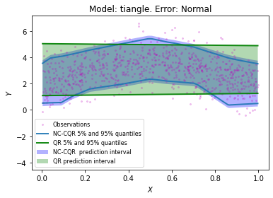
3. Model 3. “Triangle”: Triangular function

   $$Y=(4-3|X-0.5|)+\varepsilon.$$ (S35)

4. Model 4. “Discontinuous”: Discontinuous function

   $$Y=5X\mathbbm{1}(X\leq 0.5)+5(X-1)\mathbbm{1}(X>0.5)+\varepsilon.$$ (S36)

For the above models, we try different error distributions:

• $\varepsilon$ follows the standard normal distribution, i.e., $\varepsilon\sim N(0,1)$, denoted by Normal.

• Conditional on $X=x$, $\varepsilon$ follows a normal distribution with mean 0 and variance increasing in $x$, i.e., $\varepsilon\mid X=x\sim N(0,e^{(x-0.5)^{2}})$, denoted by Exp.

• Conditional on $X=x$, $\varepsilon$ follows a normal distribution with mean 0 and variance depending on $x$ via a sine function, i.e., $\varepsilon\mid X=x\sim N(0,\frac{1}{4}\sin(\pi x))$, denoted by Sin.

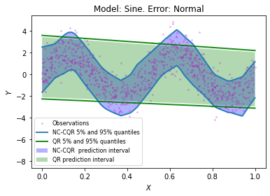
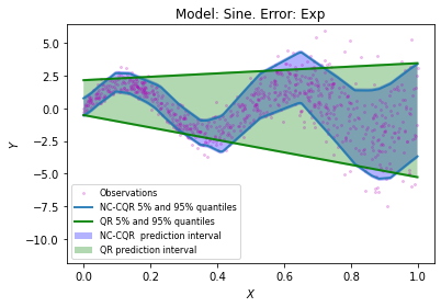
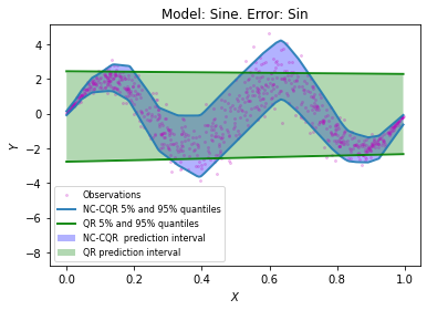
We construct $90\%$ conformal prediction intervals based on our proposed NC-CQR in (12) in the main context and the linear quantile regression (QR) method in (16) in the main context for univariate models 1-4 with $\alpha=0.1$, $\tau_{1}=0.05$ and $\tau_{2}=0.95$. The prediction intervals based on NC-CQR and linear QR under different settings are displayed in Figure S5. In addition, we perform 50 replications by randomly splitting the training data $50$ times, and calculate the average statistics and their standard deviations. The comparison between NC-CQR and QR intervals under different univariate settings is given in Table S1, which shows that on average the NC-CQR interval can achieve valid coverage with shorter average length compared to the QR interval. It is worth noting that although the theoretical guarantees of the accuracy in Lemma 4.2 and Theorem 4.5 require that the target quantile function is a Hölder smooth function in Condition (C3), our NC-CQR method still works reasonably well in terms of valid coverage rate and accuracy under setting 4 with a discontinuous target quantile function.

Table S1: Comparison of NC-CQR and QR interval under univariate settings.

	Error	$Normal$
Setting	Method	Length	Coverage	$Q_{1-\alpha}(E,\mathcal{I}_{2})$
Sine	NC-CQR	3.464(0.096)	90.5%(0.016)	0.085(0.092)
	QR	5.484(0.057)	90.7%(0.010)	0.068(0.066)
2-phase	NC-CQR	9.854(0.276)	90.0%(0.011)	0.095(0.125)
	QR	10.870(0.256)	89.8%(0.009)	0.022(0.191)
Triangle	NC-CQR	3.411(0.091)	90.3%(0.014)	0.026(0.096)
	QR	3.836(0.087)	89.9%(0.015)	0.009(0.057)
Discontinuous	NC-CQR	3.521(0.081)	90.8%(0.015)	0.061(0.080)
	QR	5.234(0.112)	89.6%(0.010)	0.036(0.109)
	Error	$Exp$
Setting	Method	Length	Coverage	$Q_{1-\alpha}(E,\mathcal{I}_{2})$
Sin	NC-CQR	3.857(0.097)	90.3%(0.016)	0.054(0.064)
	QR	5.746(0.090)	90.2%(0.013)	0.001(0.087)
2-phase	NC-CQR	14.739(0.550)	90.6%(0.014)	0.047(0.059)
	QR	16.543(0.482)	90.3%(0.011)	0.066(0.104)
Triangle	NC-CQR	3.807(0.107)	90.0%(0.013)	0.050(0.059)
	QR	4.407(0.094)	89.9%(0.007)	0.020(0.044)
Discontinuous	NC-CQR	3.851(0.066)	90.4%(0.007)	0.040(0.074)
	QR	5.627(0.103)	90.2%(0.012)	0.060(0.056)
	Error	$Sin$
Setting	Method	Length	Coverage	$Q_{1-\alpha}(E,\mathcal{I}_{2})$
Sin	NC-CQR	2.167(0.068)	89.8%(0.014)	0.034(0.041)
	QR	4.838(0.053)	90.1%(0.012)	0.032(0.057)
2-phase	NC-CQR	6.566(0.208)	90.2%(0.011)	0.078(0.071)
	QR	7.967(0.442)	90.1%(0.011)	0.012(0.044)
Triangle	NC-CQR	2.149(0.039)	89.6%(0.012)	0.026(0.028)
	QR	2.853(0.070)	89.2%(0.017)	0.009(0.060)
Discontinuous	NC-CQR	2.211(0.040)	90.1%(0.008)	0.009(0.032)
	QR	4.758(0.075)	90.7%(0.016)	0.010(0.041)

Notes: “Length” denotes the average length defined in (S29); “Coverage” denotes the coverage rate define in (S30); $Q_{1-\alpha}(E,\mathcal{I}_{2})$ is the $(1-\alpha)$-th empirical quantile of the conformity score defined in (S28).

In addition, we also simulated data under Model 5 to show the power of non-crossing penalty.

• Model 5. Double sine function:

  $$Y=5v^{\top}\sin(2\pi X)+5(1-v)^{\top}\sin(-2\pi X)+\varepsilon,$$ (S37)

  where $v\sim Bernoulli(0.5,n)$ and conditional on $X=x$, $\varepsilon$ follows a normal distribution with mean 0 and variance depending on $x$ via a sine function, i.e., $\varepsilon\mid X=x\sim N(0,\frac{1}{4}\sin(\pi x))$.

Fig. 1 in the paper is generated from Model 5 with Sin error. It presents 6 distinct estimated quantiles by CQR method (right) and NC-CQR method (left) where there are crossing parts at the right-hand side and there is no crossing at the left-hand side.

(a) Estimations under Model 1

(b) Estimations under Model 2

(c) Estimations under Model 3

(d) Estimations under Model 4

Figure S5: The comparison between NC-CQR and QR under univariate models 1-4

B.3 Multivariate models

We consider a multivariate setting with heterogeneous error in the simulation studies.

1. Model 6. Single index model with heterogeneous error:

   $$Y=\exp\left(\theta^{\top}X\right)+\varepsilon,\ \ \ \ \varepsilon\mid X\sim N(0,\sin(\pi X)),$$ (S38)

   where $X$ follows Uniform $[0,1]^{d}$ with independent components, and the true value of the parameter vector $\theta\in\mathbb{R}^{d}$ is fixed to be a subvector of the first $d$ value of

   $$\theta*= \left(0.29,0.15,-0.34,-0.62,-1.56,-1.51,-0.94,0.01,0.08,1.02,1.95,-2.35,2.44,\right.$$

   $$\left.0.35,-0.01,-1.09,-0.49,2.11,1.44,-0.51,-0.33,3.14,0.95,0.39,-0.16\right)^{\top}.$$

We consider different dimensions with $d=5,10,15,20,25$, to investigate how the dimensionality of the input affects the overall performance. We construct $80\%$ conformal intervals by our proposed NC-CQR and the CQR (Romano et al.,, 2019). Set $\alpha=0.2$, $\tau_{1}=0.1$ and $\tau_{2}=0.9$. The conformal band is then constructed based on the estimated $10\%$ and $90\%$ quantiles respectively. The simulation results are reported in Table S2, which shows that the estimated quantile curves by our proposed NC-CQR have fewer crossing than the CQR method. While for conformal intervals, after making use of the conformity score in (S28), we observe that there is nearly no crossing in both CQR and NC-CQR, but CQR interval has a larger $(1-\alpha)$-th quantile of the conformity score and larger length than our proposed NC-CQR interval. We give a 3D visualization of the conformal intervals by our proposed NC-CQR and the CQR method with $d=2$ in Figure 2 in main context. Both NC-CQR and CQR intervals achieve $80\%$ coverage rate, and the crossing rate of the NC-CQR and CQR interval are $0\%$ and $0.1\%$ respectively. The average lengths of NC-CQR interval and CQR interval are $1.675$ and $1.681$ respectively, which shows that the NC-CQR interval is slightly shorter.

Table S2: Comparison between NC-CQR and CQR under multivariate settings.

$d$	Method	CR-NN	CR-CI	Coverage	Length	$Q_{1-\alpha}(E,\mathcal{I}_{2})$
$5$	CQR	$0.1\%$	$0.0\%$	$77.5\%$	$2.73$	$0.34$
	NC-CQR	$0.0\%$	$0.0\%$	$80.8\%$	$2.91$	$0.20$
$10$	CQR	$0.2\%$	$0.0\%$	$79.3\%$	$3.02$	$0.75$
	NC-CQR	$0.1\%$	$0.0\%$	$80.3\%$	$3.00$	$0.56$
$15$	CQR	$0.2\%$	$0.0\%$	$79.4\%$	$2.77$	$0.86$
	NC-CQR	$0.0\%$	$0.0\%$	$79.6\%$	$2.01$	$0.56$
$20$	CQR	$0.5\%$	$0.0\%$	$81.1\%$	$2.66$	$1.15$
	NC-CQR	$0.1\%$	$0.0\%$	$80.0\%$	$2.61$	$1.01$
$25$	CQR	$0.7\%$	$0.0\%$	$78.2\%$	$2.53$	$1.07$
	NC-CQR	$0.1\%$	$0.0\%$	$78.3\%$	$2.64$	$0.22$

Notes: “CR-NN” denotes the crossing rate of neural network estimates defined in (S31); “CR-CI” denotes the crossing rate of the conformal interval defined in (S32); “Length” denotes the average length defined in (S29); $Q_{1-\alpha}(E,\mathcal{I}_{2})$ is the $(1-\alpha)$-th empirical quantile of the conformity score defined in (S28). Each presented result is the average of $10$ experiments.

B.4 Real data analysis

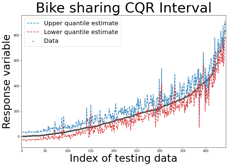
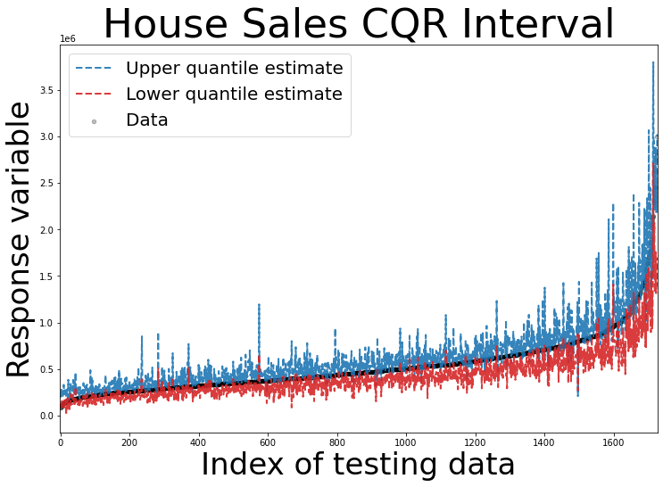
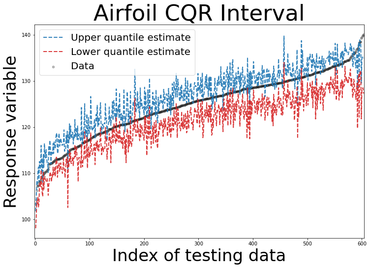
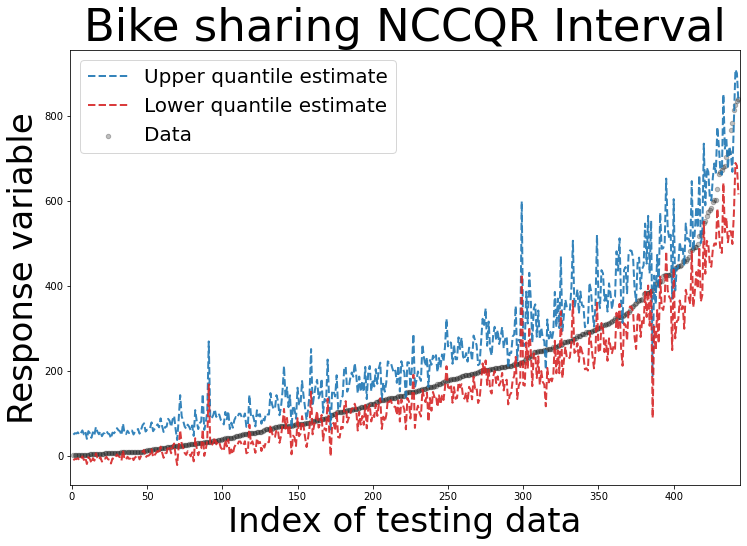
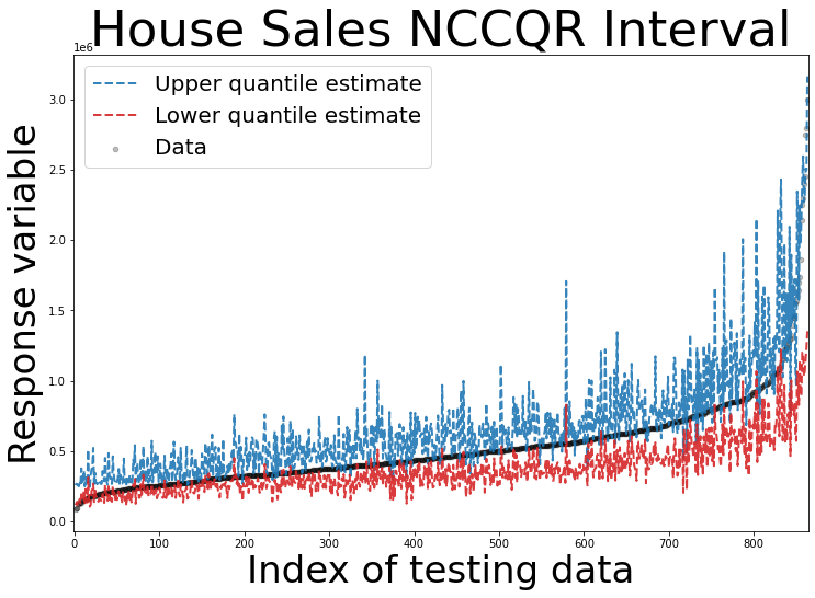
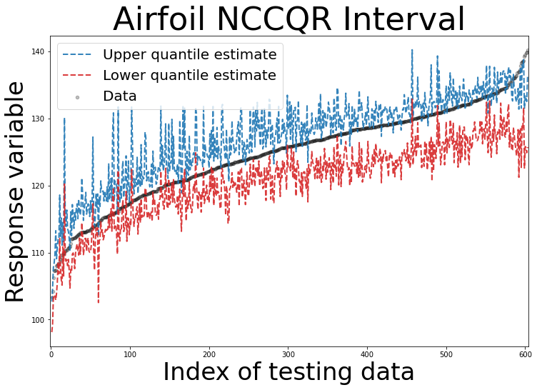
In this subsection, first, we apply the NC-CQR method to the housing sales data in King County, USA. The dataset contains $n=21,563$ sold houses data between May 2014 and May 2015. For each house sold, the data consists of $21$ attributes including housing price, the number of bedrooms, bathrooms, size, view, etc. The prediction target is the housing price. We exclude nominal variables including house id, date, and zip code, and intend to predict the housing price from the remaining $17$ attributes and construct an $80\%$ prediction interval corresponding to the observations. We also apply the proposed method to Bike sharing dataset with $n=10,886,d=18$ and the airfoil dataset with $n=1,503,d=5$. The goal of the analysis on the Bike sharing dataset is to predict the interval of the total number of rental bikes number given the $18$ related attributes such as weather and season. The goal of the analysis on the airfoil dataset is to construct a prediction interval of the scaled sound pressure level given six attributes such as the angle of the attack. We let $\alpha=0.2$, $\tau_{1}=0.1$ and $\tau_{2}=0.9$. The conformal band is constructed based on the estimated $10\%$ and $90\%$ quantiles respectively. We randomly select $T=0.4n$ testing data from $n$ samples. And we evenly split the remaining samples into two subsets: a proper training set ${\mathcal{I}}_{1}$ with $n_{\rm train}=0.3n$ samples and calibration set ${\mathcal{I}}_{2}$ with $n_{\rm cal}=0.3n$ samples.

According to Algorithm 1, we construct the conformal interval by (12) in the main context and the length and coverage rate are computed according to (S29) and (S30). Also, we compare the NC-CQR to CQR and QR described in subsection 4.1. We present the length in (S29) and the $(1-\alpha)$-th empirical quantile of the conformity score, denoted by $Q_{1-\alpha}(E,\mathcal{I}_{2})$, the coverage rate in (S30), CR-NN in (S31) and CR-CI in (S32) in Table S3. Table S3 shows that all three methods achieve valid coverage in the housing price prediction. In addition, NC-CQR avoids the crossing problem of lower and upper bounds in CQR. Besides, the average length of the prediction interval in NC-CQR is smaller than that of the QR method, which means that the NC-CQR is more accurate than QR.

Table S3: Comparison of different methods on three datasets.

			House sales
Method	CR-NN	CR-CI	Coverage	Length	$Q_{1-\alpha}(E,\mathcal{I}_{2})$
NC-CQR	$0.0\%$	$0.0\%$	$79.4\%$	$3.10$	$-0.01$
CQR	$0.2\%$	$0.0\%$	$80.8\%$	$2.15$	$0.02$
QR	$0.0\%$	$0.0\%$	$76.3\%$	$4.52$	$0.27$
			Bike sharing
Method	CR-NN	CR-CI	Coverage	Length	$Q_{1-\alpha}(E,\mathcal{I}_{2})$
NC-CQR	$0.0\%$	$0.0\%$	$81.8\%$	$89.42$	$31.14$
CQR	$0.2\%$	$0.0\%$	$82.1\%$	$84.02$	$24.64$
QR	$0.0\%$	$0.0\%$	$76.3\%$	$123.45$	$25.57$
			Air foil
Method	CR-NN	CR-CI	Coverage	Length	$Q_{1-\alpha}(E,\mathcal{I}_{2})$
NC-CQR	$0.0\%$	$0.0\%$	$81.1\%$	$6.64$	$0.84$
CQR	$0.0\%$	$0.0\%$	$78.1\%$	$5.90$	$0.96$
QR	$0.0\%$	$0.0\%$	$77.4\%$	$11.69$	$-0.34$

Notes: “CR-NN” denotes the crossing rate of neural network estimates defined in (S31); “CR-CI” denotes the crossing rate of the conformal interval defined in (S32); “Coverage” denotes the coverage rate defined in (S30); “Length” denotes the average length defined in (S29); $Q_{1-\alpha}(E,\mathcal{I}_{2})$ is the $(1-\alpha)$-th empirical quantile of the conformity score defined in (S28; For house sales table, the scale of Length and $Q_{1-\alpha}(E,\mathcal{I}_{2})$ is $\times 10^{5}$.

B.5 Tuning Parameter Selection

In the penalized loss function (6) in the paper, the tuning parameter $\lambda$ determines the extent of penalization. The popular One Standard Error Rule (1se rule) is used with cross-validation (CV) to compare models with different numbers of parameters in order to select the most parsimonious model with low error.

The idea of $K$-fold cross-validation is to split the data into $K$ roughly equal-sized parts: $D_{1},\ldots,D_{K}$. For the $k$-th part where $k=1,2,\ldots,K$, we train the model on $K-1$ data set $\left(x_{i},y_{i}\right),i\notin D_{k}$ and the conduct the evaluation on $\left(x_{i},y_{i}\right),i\in D_{k}$. Now consider $\lambda$ in a set of candidate tuning parameter $\left\{\lambda_{1},\ldots,\lambda_{m}\right\}$, we obtain the estimate $(\hat{f}_{1,\lambda}^{(-k)},\hat{f}_{2,\lambda}^{(-k)})$ on the training set $\left(x_{i},y_{i}\right),i\notin D_{k}$. Then we calculate the summation of the average length and the number of crossing points (ALC) on the validation set defined as

$$ALC_{k}(\lambda)=\frac{1}{|D_{k}|}\sum_{i\in D_{k}}\left|\hat{f}_{2,\lambda}^{(-k)}\left(x_{i}\right)-\hat{f}_{1,\lambda}^{(-k)}\left(x_{i}\right)\right|+\sum_{i\in D_{k}}\mathbbm{1}_{\hat{f}_{1,\lambda}^{(-k)}\left(x_{i}\right)<\hat{f}_{2,\lambda}^{(-k)}\left(x_{i}\right)}.$$ (S39)

For each tuning parameter value $\lambda$, we compute the average error over all folds:

$$ALC(\lambda)=\frac{1}{K}\sum_{k=1}^{K}ALC_{k}(\lambda)$$

We then choose the value of the tuning parameter that minimizes the above-average error, $\hat{\lambda}_{\min}=\operatorname{argmin}_{\lambda\in\left\{\lambda_{1},\ldots,\lambda_{m}\right\}}ALC(\lambda).$ By the proposed tuning parameter selection, we can choose the $\lambda$ that can both avoid the crossing problem and achieve a narrow interval.

References

- Anthony et al., (1999) Anthony, M., Bartlett, P. L., Bartlett, P. L., et al. (1999). Neural network learning: Theoretical foundations, volume 9. cambridge university press Cambridge.
- Barber et al., (2021) Barber, F. R., Candes, E. J., Ramdas, A., and Tibshirani, R. J. (2021). The limits of distribution-free conditional predictive inference. Information and Inference: A Journal of the IMA, 10(2):455–482.
- Bartlett et al., (2019) Bartlett, P. L., Harvey, N., Liaw, C., and Mehrabian, A. (2019). Nearly-tight vc-dimension and pseudodimension bounds for piecewise linear neural networks. The Journal of Machine Learning Research, 20(1):2285–2301.
- Belloni et al., (2019) Belloni, A., Chernozhukov, V., and Kato, K. (2019). Valid post-selection inference in high-dimensional approximately sparse quantile regression models. Journal of the American Statistical Association, 114(526):749–758.
- Bondell et al., (2010) Bondell, H. D., Reich, B. J., and Wang, H. (2010). Noncrossing quantile regression curve estimation. Biometrika, 97(4):825–838.
- Brando et al., (2022) Brando, A., Center, B. S., Rodriguez-Serrano, J., Vitria, J., et al. (2022). Deep non-crossing quantiles through the partial derivative. In International Conference on Artificial Intelligence and Statistics, pages 7902–7914. PMLR.
- He, (1997) He, X. (1997). Quantile curves without crossing. The American Statistician, 51(2):186–192.
- Jiao et al., (2021) Jiao, Y., Shen, G., Lin, Y., and Huang, J. (2021). Deep nonparametric regression on approximately low-dimensional manifolds. arXiv 2104.06708.
- Kivaranovic et al., (2020) Kivaranovic, D., Johnson, K. D., and Leeb, H. (2020). Adaptive, distribution-free prediction intervals for deep networks. In International Conference on Artificial Intelligence and Statistics, pages 4346–4356. PMLR.
- Koenker, (1984) Koenker, R. (1984). A note on l-estimates for linear models. Statistics & probability letters, 2(6):323–325.
- Koenker, (2005) Koenker, R. (2005). Quantile Regression. Econometric Society Monographs. Cambridge University Press.
- Lei et al., (2018) Lei, J., G’Sell, M., Rinaldo, A., Tibshirani, R. J., and Wasserman, L. (2018). Distribution-free predictive inference for regression. Journal of the American Statistical Association, 113(523):1094–1111.
- Lei et al., (2013) Lei, J., Robins, J., and Wasserman, L. (2013). Distribution-free prediction sets. Journal of the American Statistical Association, 108(501):278–287.
- Lei and Wasserman, (2014) Lei, J. and Wasserman, L. (2014). Distribution-free prediction bands for non-parametric regression. Journal of the Royal Statistical Society: Series B: Statistical Methodology, pages 71–96.
- Neocleous and Portnoy, (2008) Neocleous, T. and Portnoy, S. (2008). On monotonicity of regression quantile functions. Statistics & probability letters, 78(10):1226–1229.
- Papadopoulos, (2008) Papadopoulos, H. (2008). Inductive conformal prediction: Theory and application to neural networks. INTECH Open Access Publisher Rijeka.
- Papadopoulos et al., (2002) Papadopoulos, H., Proedrou, K., Vovk, V., and Gammerman, A. (2002). Inductive confidence machines for regression. In European Conference on Machine Learning, pages 345–356. Springer.
- Romano et al., (2019) Romano, Y., Patterson, E., and Candes, E. (2019). Conformalized quantile regression. Advances in Neural Information Processing Systems, 32:3543–3553.
- Sesia and Candès, (2020) Sesia, M. and Candès, E. J. (2020). A comparison of some conformal quantile regression methods. Stat, 9(1):e261.
- Shen et al., (2021) Shen, G., Jiao, Y., Lin, Y., Horowitz, J. L., and Huang, J. (2021). Deep quantile regression: Mitigating the curse of dimensionality through composition. arXiv preprint arXiv:2107.04907.
- Tagasovska and Lopez-Paz, (2019) Tagasovska, N. and Lopez-Paz, D. (2019). Single-model uncertainties for deep learning. Advances in Neural Information Processing Systems, 32.
- Vovk, (2012) Vovk, V. (2012). Conditional validity of inductive conformal predictors. In Asian conference on machine learning, pages 475–490. PMLR.
- Vovk et al., (2005) Vovk, V., Gammerman, A., and Shafer, G. (2005). Algorithmic learning in a random world. Springer Science & Business Media.
- Zeni et al., (2020) Zeni, G., Fontana, M., and Vantini, S. (2020). Conformal prediction: a unified review of theory and new challenges. arXiv preprint arXiv:2005.07972.