Generalized interacting Barrow Holographic Dark Energy: cosmological predictions and thermodynamic considerations

Abstract

We construct a generalized interacting model of Barrow Holographic Dark Energy (BHDE) with infrared cutoff being given by the Hubble horizon. We analyze the cosmological evolution of a flat Friedmann-Lemaître-Robertson-Walker Universe filled by pressureless dark matter, BHDE and radiation fluid. The interaction between the dark sectors of the cosmos is assumed of non-gravitational origin and satisfying the second law of thermodynamics and Le Chatelier-Braun principle. We study the behavior of various model parameters, such as the BHDE density parameter, the equation of state parameter, the deceleration parameter, the jerk parameter and the square of sound speed. We show that our model satisfactorily retraces the thermal history of the Universe and is consistent with current observations for certain values of parameters, providing an eligible candidate to describe dark energy. We finally explore the thermodynamics of our framework, with special focus on the validity of the generalized second law.

I Introduction

It is nowadays established experimentally that our Universe is experiencing an accelerated expansion Supern ; Supernbis ; Supernter ; Supernquar ; Supernquin . Despite the intensive theoretical and observational studies, the origin of this phenomenon is yet to be understood, leaving room for disparate explanations. Among the various scenarios, a plausible mechanism is the existence of an exotic form of energy with large negative pressure - the Dark Energy (DE) - which should affect the Universe on large scales. However, the true nature of this entity remains unknown, and a vast number of theoretical models have been proposed to shed light on its properties Peebles:1987ek ; Ratra:1987rm ; Wetterich:1987fm ; Frieman:1995pm ; Turner:1997npq ; Caldwell:1997ii ; Armendariz-Picon:2000nqq ; Amendola:1999er ; Armendariz-Picon:2000ulo ; Kamenshchik:2001cp ; Caldwell:1999ew ; Caldwell:2003vq ; Nojiri:2003vn ; Feng:2004ad ; Guo:2004fq ; Elizalde:2004mq ; Nojiri:2005sx ; Deffayet:2001pu ; Sen:2002in ; Zhangov .

In this context, a valuable approach is the so called Holographic Dark Energy (HDE) model Cohen:1998zx ; Horava:2000tb ; Thomas:2002pq ; Li:2004rb ; Hsu:2004ri ; Huang:2004ai ; Wang:2005ph ; Setare:2006sv ; Granda ; Sheykhi:2011cn ; Bamba:2012cp ; Ghaffari:2014pxa ; Wang:2016och ; Moradpour:2020dfm , which is based on the holographic principle and the use of Bekenstein-Hawking (BH) area law Beke for the entropy on the Universe horizon. Cosmological applications of HDE have been extensively considered in literature Enqvist:2004ny ; Setare:2007hq ; Sriva . Nevertheless, the shortcomings of this model in describing the history of the Universe have motivated tentative changes over the years. For instance, several extensions have been developed to accommodate non-additive Tavayef:2018xwx ; Saridakis:2018unr ; Nojiri:2019skr , relativistic Drepanou:2021jiv ; Hernand and quantum-like BarSar ; Dabrowski:2020atl ; Sheykhi:2021fwh ; Adhikary:2021xym ; Nojiri:2021jxf corrections to BH entropy. The ensuing frameworks are referred to as Tsallis Tavayef:2018xwx ; Saridakis:2018unr ; Nojiri:2019skr ; Luciano:2022ely , Kaniadakis Drepanou:2021jiv ; Hernand ; ModKa and Barrow BarSar ; Dabrowski:2020atl ; Sheykhi:2021fwh ; Adhikary:2021xym ; Nojiri:2021jxf ; LucianoBarrow ; Anagnostopoulos:2020ctz ; GhaffariLuc ; LucTherm HDE, respectively, and have been shown to well fit experimental data for certain values of the model parameters.

In various cosmological scenarios, it is typically assumed that dark energy interacts with dark matter (DM) ReviewDM ; Addazi , the existence of which is invoked to explain the observed flatness of the rotation curves of spiral galaxies. Besides, such an interaction might play a non-trivial rôle in solving some open problems in modern Cosmology, such as the coincidence problem Amendola ; Bolotin:2013jpa and the current tension on the local value of the Hubble constant DiVale ; Kumar:2017dnp . Therefore, cosmological models involving interactions between the dark sectors of the cosmos turn out to be particularly compelling and deserve special attention.

Along this line, interacting models of HDE based on non-extensive Tsallis entropy have been investigated in a variety of contexts, ranging from higher dimensional Cosmology Saha , to the Brans-Dicke Cosmology BDCosmo and DGP brane-world DGP . Recently, a theoretical model of generalized interacting Tsallis HDE has been studied in Mamon:2020wnh along with its thermodynamic implications. Inspired by this analysis, the dynamics of the interacting HDE based on Barrow entropy (Barrow Holographic Dark Energy, BHDE) has been proposed in Mamon:2020spa for a spatially flat Friedmann-Lemaître-Robertson-Walker (FLRW) Universe composed of pressureless DM and BHDE.

Starting from the above premises, in this manuscript we explore the consequences of the interacting BHDE model in a more general scenario. In a recent work by one of the authors LucTherm , the cosmic evolution and thermal stability of BHDE have been studied in nonflat Friedmann-Robertson-Walker geometry by considering a particular form for the interaction and neglecting the radiation content of the Universe. Here we extend the above analysis to the case of the most general interaction satisfying Le Chatelier-Braun principle and also take account of radiation fluid effects, which are particularly relevant in the early stages of Universe existence. In this sense, our work also extends the results of Mamon:2020spa , where a Universe filled up only with dark matter and energy has been considered. In this background, we analyze the behavior of the BHDE density parameter, the deceleration parameter, the jerk parameter and the BHDE equation of state parameter, as well as the classical stability and thermodynamic nature of our model, showing that our generalized scenario has a phenomenology richer than the one of Mamon:2020spa ; LucTherm . This clearly offer fresh insights toward a more comprehensive understanding of the intimate nature of dark energy. We also prove that the present framework is consistent with recent observations, thus providing a good candidate for the description of DE.

The remainder of the work is organized as follows: in the next Section we describe the interacting BHDE model. In particular, we study the cosmological evolution of some characteristic parameters of the model for a Universe filled by pressureless DM and BHDE. In Sec. III we extend this analysis to the case where the radiation fluid is also present. Sec. IV is devoted to investigate the thermodynamic implications of this generalized BHDE model. Conclusions and outlook are finally summarized in Sec. V. Throughout the entire manuscript, we work in units where $\hbar=k_{B}=c=1$, while we keep the gravitational constant $G$ explicit. Furthermore, we use the mostly negative signature for the metric.

II Interacting BHDE model with Hubble scale as IR cutoff

Let us start by describing the framework of the interacting BHDE model and its cosmological implications. BHDE is based upon the holographic principle with the following modified entropy-area law for the Universe horizon BarSar

$$S_{\Delta}\,=\,\left(\frac{A}{A_{0}}\right)^{1+\Delta/2}\,,$$ (1)

where $A$ is the area enclosed by the horizon surface and $A_{0}=4G$ the Planck area. Although this relation was originally proposed by Barrow to accommodate quantum-gravitational effects on the horizon of black holes BarrowBH , it can also be applied in the cosmological framework based on the gravity-thermodynamic conjecture BarSar ; Dabrowski:2020atl ; Sheykhi:2021fwh ; Adhikary:2021xym ; Nojiri:2021jxf . In this way, extra corrections appear in the Standard Model of Cosmology, namely on the Friedmann equations. Such terms are parameterized by the exponent $0\leq\Delta\leq 1$, where $\Delta=0$ gives the standard Bekenstein-Hawking limit, while $\Delta=1$ corresponds to the maximal horizon deformation. In passing, we mention that constraints on $\Delta$ have been derived in Anagnostopoulos:2020ctz ; Leon:2021wyx ; Barrow:2020kug ; Jusufi:2021fek ; Dabrowski:2020atl ; Saridakis:2020cqq ; Luciano:2022pzg ; Vagnozzi:2022moj . Furthermore, the possibility of a running $\Delta$ has been discussed in DiGennaro:2022ykp .

We now observe that the usage of Barrow entropy (1) leads to the following holographic dark energy density BarSar

$$\rho_{D}=CL^{\Delta-2}\,,$$ (2)

where $C$ is an unknown parameter with dimensions $[L]^{-2-\Delta}$ and $L$ is the characteristic size of the system. It is worth noticing that, for $\Delta=0$, the above relation reduces to the standard HDE Cohen:1998zx ; Horava:2000tb ; Thomas:2002pq ; Li:2004rb ; Hsu:2004ri ; Huang:2004ai ; Wang:2005ph ; Setare:2006sv ; Granda ; Sheykhi:2011cn ; Bamba:2012cp ; Ghaffari:2014pxa ; Wang:2016och ; Moradpour:2020dfm , provided that $C=3c^{2}m_{p}^{2}$, where $m_{p}$ is the reduced Planck mass and $c$ a dimensionless constant (not to be confused with the speed of light). Conversely, in the case where deformations effects are taken into account (i.e. $\Delta\neq 0$), BHDE gives rise to a more general framework than HDE BarSar ; Dabrowski:2020atl ; Sheykhi:2021fwh ; Adhikary:2021xym ; Nojiri:2021jxf .

By considering the Hubble horizon $L=H^{-1}$ as the IR cutoff, the energy density of BHDE can be rewritten as

$$\rho_{D}=CH^{2-\Delta}\,.$$ (3)

This relation provides the crucial ingredient of our next analysis.

Let us assume that the Universe is homogenous, isotropic and spatially flat on large scales, so that it can be described by the standard Friedmann-Lemaître-Robertson-Walker (FLRW) metric

$$ds^{2}=dt^{2}-a^{2}(t)\left(dr^{2}+r^{2}d\Omega^{2}\right),$$ (4)

where $a(t)$ is the scale factor depending on the cosmic time $t$ and $r,\Omega$ are the radial and angular coordinates, respectively. Under the further assumption that the Universe be filled by pressureless DM and BHDE of densities $\rho_{m}$ and $\rho_{D}$, respectively, Friedmann equations take the standard form

$$H^{2} = \frac{1}{3m_{p}^{2}}\left(\rho_{m}+\rho_{D}\right),$$ (5)

$$\dot{H} = -\frac{1}{2m_{p}^{2}}\left(\rho_{m}+\rho_{D}+p_{D}\right),$$ (6)

where $H=\dot{a}/a$ is the Hubble parameter and the overdot denotes derivative respect to $t$. The pressure of BHDE has been indicated by $p_{D}$ and is related to the energy density $\rho_{D}$ via the equation of state (EoS)

$$\omega_{D}\equiv\frac{p_{D}}{\rho_{D}}\,,$$ (7)

where $\omega_{D}$ is the so called EoS parameter.

We can also introduce the fractional energy density parameters of DM ($\Omega_{m}$) and BHDE ($\Omega_{D}$) as

$$\Omega_{m} = \frac{\rho_{m}}{\rho_{c}}\,,$$ (8)

$$\Omega_{D} = \frac{\rho_{D}}{\rho_{c}}=\frac{C}{3m_{p}^{2}}H^{-\Delta}\,,$$ (9)

where

$$\rho_{c}=3m_{p}^{2}H^{2}$$ (10)

is the critical energy density. In this way, Eq. (5) can be equivalently rewritten as $\Omega_{m}+\Omega_{D}=1$. Moreover, we define the ratio of the energy densities as $r=\rho_{m}/\rho_{D}=\Omega_{m}/\Omega_{D}$.

Let us now assume that DM and BHDE nontrivially interact with each other. Denoting by $Q$ the rate of energy exchange, the conservation equation for the dark sectors of the Universe can be written as follows

$$\dot{\rho}_{m}+3H\rho_{m}=Q\,,$$ (11a)

$$\dot{\rho}_{D}+3H\left(1+\omega_{D}\right)\rho_{D}=-Q\,.$$ (11b)

Some comments on the sign and functional form of the interaction $Q$ are in order here. First, we notice that for $Q>0$, energy flows from BHDE to DM, while the opposite happens for $Q<0$. Second, while many interactions have been proposed to describe the dynamics of the Universe, the exact form of $Q$ is still unknown (see Q1 ; Q2 ; Q3 ; Q4 for more details). Following Mamon:2020spa ; Mamon:2020wnh , hereafter we assume

$$Q=3H\left(b_{1}^{2}\rho_{m}+b_{2}^{2}\rho_{D}\right),$$ (12)

where the model parameters $b_{1}$ and $b_{2}$ are dimensionless constants. This form of $Q$ is largely used in the literature for different choices of $b_{1}$ and $b_{2}$. Since in our setting the coefficients $b_{1}^{2}$ and $b_{2}^{2}$ are always positive, we have $Q>0$, consistently with the validity of the second law of thermodynamics and Le Chatelier-Braun principle Q2 . We also require $b_{1}^{2}\neq b_{2}^{2}$ and $b_{1}^{2},b_{2}^{2}\ll 1$ for observational reasons Chimento .

Now, by taking the time derivative of Eq. (5) combined with Eqs. (11), we obtain after some algebra

$$\frac{\dot{H}}{H^{2}}=-\frac{3}{2}\Omega_{D}\left(1+\omega_{D}+r\right).$$ (13)

In a similar fashion, the derivative of Eq. (3) leads to

$$\omega_{D}=\frac{-\frac{\Delta}{2}-\frac{b_{1}^{2}}{\Omega_{D}}+b_{1}^{2}-b_{2}^{2}}{1-\left(1-\frac{\Delta}{2}\right)\Omega_{D}}\,.$$ (14)

Notice that this function is divergent for $\Omega_{D}={(1-\Delta/2)}^{-1}$. However, since by definition $\Omega_{D}<1$, such condition cannot be satisfied by any $0\leq\Delta\leq 1$.

The dynamical evolution of the BHDE density parameter $\Omega_{D}$ can be obtained by deriving Eq. (9) respect to $t$ and then resorting to Eqs. (13) and (14). We get the following differential equation

$$\Omega^{\prime}_{D}=\frac{3\Delta\Omega_{D}}{2}\left[\frac{1-\Omega_{D}-b_{1}^{2}+\left(b_{1}^{2}-b_{2}^{2}\right)\Omega_{D}}{1-\left(1-\frac{\Delta}{2}\right)\Omega_{D}}\right],$$ (15)

where the prime denotes derivative respect to $\log a$, i.e. $\Omega^{\prime}_{D}=\frac{d\Omega_{D}}{d(\log a)}$. For our next purposes, we also remind that

$$\frac{1}{a}=\frac{1+z}{a_{0}}\,,$$ (16)

where $z$ denotes the redshift and $a_{0}$ is the present value of the scale factor. Here, we take $a_{0}=1$, so that $a^{-1}=1+z$.

In order to determine the behavior of BHDE density parameter, we solve Eq. (15) by numerical integration. Results are shown in Fig. 2 and Fig. 2 for different values of the interaction terms $b_{1}^{2},b_{2}^{2}$ and Barrow parameter $\Delta$, respectively. From these plots, it is evident that $\Omega_{D}$ increases monotonically from zero at early times to unity in the far future (i.e. $z\rightarrow-1$), indicating an evolution toward a completely dark energy dominated epoch predicted by this model.

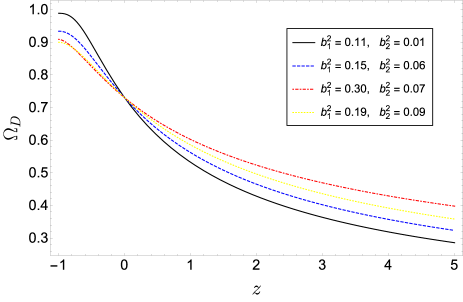
Figure 1: The evolution of $\Omega_{D}$ versus $z$ for different values of $b_{1}^{2}$ and $b_{2}^{2}$. We set $\Delta=0.5$ and $\Omega_{D}^{0}=0.73$ as initial condition.

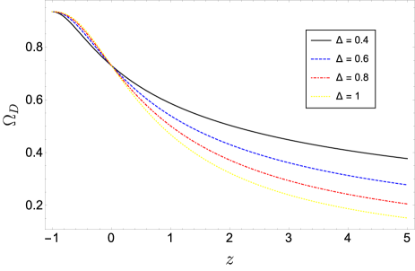
Figure 2: The evolution of $\Omega_{D}$ versus $z$ for different values of $\Delta$. We set $b_{1}^{2}=0.15$, $b_{2}^{2}=0.06$ and $\Omega_{D}^{0}=0.73$ as initial condition.

From Eq. (14), we can infer the dynamics of the EoS parameter $\omega_{D}$. Specifically, from Fig. 4 we see that $\omega_{D}$ always lies in the quintessence regime ($-1<\omega_{D}<-1/3$) at present (i.e. $z=0$) for the considered values of $b_{1}^{2},b_{2}^{2}$. However, it first approaches the cosmological constant behavior ($\omega_{D}=-1$) and then crosses the phantom line ($\omega_{D}<-1$) in the far future (i.e. $z\rightarrow-1$) for increasing $b_{1}^{2},b_{2}^{2}$. The same profile is exhibited by varying the Barrow parameter $\Delta$ and keeping $b_{1}^{2},b_{2}^{2}$ fixed (see Fig. 4). To check the observational consistency of our model, we can also estimate the value of the EoS parameter at present epoch. From Fig. 4, it is found to satisfy $-0.90\leq\omega_{D_{0}}\leq-0.64$, while Fig. 4 gives $-0.82\leq\omega_{D_{0}}\leq-0.53$. Notice that the first interval overlaps with the recent observational constraint $-1.38<\omega_{0}<-0.89$ obtained from Planck+WP+BAO measurements Planck .

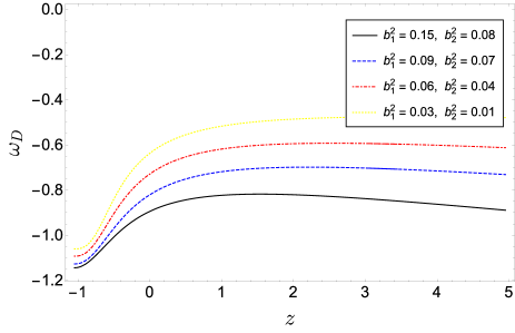
Figure 3: The evolution of $\omega_{D}$ versus $z$ for different values of $b_{1}^{2}$ and $b_{2}^{2}$. We set $\Delta=0.5$ and $\Omega_{D}^{0}=0.73$ as initial condition.

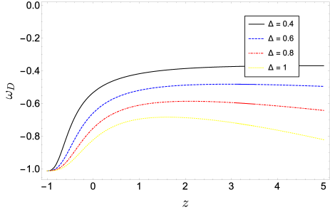
Figure 4: The evolution of $\omega_{D}$ versus $z$ for different values of $\Delta$. We set $b_{1}^{2}=0.03$, $b_{2}^{2}=0.01$ and $\Omega_{D}^{0}=0.73$ as initial condition.

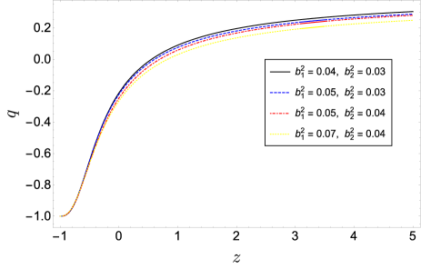
Figure 5: The evolution of $q$ versus $z$ for different values of $b_{1}^{2}$ and $b_{2}^{2}$. We set $\Delta=0.5$ and $\Omega_{D}^{0}=0.73$ as initial condition.

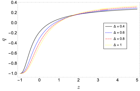
Figure 6: The evolution of $q$ versus $z$ for different values of $\Delta$. We set $b_{1}^{2}=0.05$, $b_{2}^{2}=0.04$ and $\Omega_{D}^{0}=0.73$ as initial condition.

Now, in order to explore the expansion history of the Universe, we consider the deceleration parameter

$$q=-\frac{\ddot{a}}{aH^{2}}=-1-\frac{\dot{H}}{H^{2}}\,.$$ (17)

From this relation, it follows that $q>0$ corresponds to a decelerated expansion (i.e. $\ddot{a}<0$), while $q<0$ indicates an accelerated phase ($\ddot{a}>0$). For the present model, one can show that Mamon:2020spa

$$q=\frac{-\left(1+\Delta\right)\Omega_{D}+1-3b_{1}^{2}+3\left(b_{1}^{2}-b_{2}^{2}\right)\Omega_{D}}{2\left[1-\left(1-\frac{\Delta}{2}\right)\Omega_{D}\right]}\,.$$ (18)

The evolution of $q$ versus $z$ is plotted in Fig. 6 and Fig. 6 for different values of $b_{1}^{2},b_{2}^{2}$ and $\Delta$, respectively. As we can see, the present model predicts the sequence of an early matter dominated era with a decelerated expansion (at high redshift) and a late-time DE dominated era with an accelerated phase (at low redshift), in contrast to the standard Holographic Dark Energy model. The transition redshift $z_{t}$ such that $q(z_{t})=0$, lies within the intervals $0.56\leq z_{t}\leq 0.83$ (Fig. 6) and $0.53\leq z_{t}\leq 0.96$ (Fig. 6) for the considered values of the model parameters, consistently with the recent result $0.5<z_{t}<1$ of Rapetti ; Farooq ; MamonEPJC ; MamonEPJC2 . We can also estimate the current value of the deceleration parameter as $-0.26\leq q_{0}\leq-0.20$ (Fig. 6) and $-0.46\leq q_{0}\leq-0.17$ (Fig. 6), to be compared with the observational result $q_{0}=-0.64\pm 0.22$ found in WuHu from Union2 SNIa data.

In Fig. 8 and Fig. 8 we present the evolution of the jerk parameter $j$. This is a dimensionless third derivative of the scale factor respect to the cosmic time, i.e. Blandford:2004ah ; Rapetti

$$j = \frac{1}{aH^{3}}\frac{d^{3}a}{dt^{3}}=q\left(2q+1\right)+\left(1+z\right)\frac{dq}{dz}$$

$$= \frac{1}{2}\,\Bigg{\{}-\frac{9\Delta\Omega_{D}\left(\Delta-2\right)\left[1-b_{1}^{2}+\left(b_{1}^{2}-b_{2}^{2}-1\right)\Omega_{D}\right]\left\{2b_{1}^{2}+\left(2b_{2}^{2}-2b_{1}^{2}+\Delta\right)\Omega_{D}\right\}}{\left[2+\left(\Delta-2\right)\Omega_{D}\right]^{3}}+\frac{3}{2+\left(\Delta-2\right)\Omega_{D}}$$

$$\times\,\Big{\{}-\frac{6\Delta\left(b_{1}^{2}-b_{2}^{2}\right)\left[1-b_{1}^{2}+\left(b_{1}^{2}-b_{2}^{2}-1\right)\Omega_{D}\right]\Omega_{D}+3\Delta^{2}\left[1-b_{1}^{2}+\left(b_{1}^{2}-b_{2}^{2}-1\right)\Omega_{D}\right]\Omega_{D}}{2+\left(\Delta-2\right)\Omega_{D}}\Big{\}}$$

$$+\,\Big{\{}1+\frac{3\big{\{}-\left(2b_{2}^{2}+\Delta\right)\Omega_{D}+2b_{1}^{2}\left[-1+\Omega_{D}\right]\big{\}}}{2+\left(\Delta-2\right)\Omega_{D}}\Big{\}}\Big{\{}2+\frac{3\big{\{}-\left(2b_{2}^{2}+\Delta\right)\Omega_{D}+2b_{1}^{2}\left[-1+\Omega_{D}\right]\big{\}}}{2+\left(\Delta-2\right)\Omega_{D}}\Big{\}}\Bigg{\}}\,.$$

This parameter provides us with the simplest approach to search for departures of the present model from $\Lambda$CDM, which is characterized by $j=1$. From Fig. 8 and Fig. 8, we see that $j>0$ for any redshift and approaches unity in the far future (i.e. $z\rightarrow-1$). Therefore, in this limit our model resembles $\Lambda$CDM Blandford:2004ah ; Rapetti .

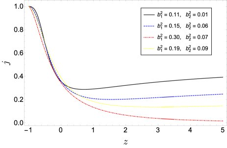
Figure 7: The evolution of $j$ versus $z$ for different values of $b_{1}^{2}$ and $b_{2}^{2}$. We set $\Delta=0.5$ and $\Omega_{D}^{0}=0.73$ as initial condition.

Figure 8: The evolution of $j$ versus $z$ for different values of $\Delta$. We set $b_{1}^{2}=0.05$, $b_{2}^{2}=0.04$ and $\Omega_{D}^{0}=0.73$ as initial condition.

In order to understand the classical stability of BHDE model, let us now focus on the square of sound speed (notice that neither this quantity nor the jerk parameter have been considered in the analysis of Mamon:2020spa ). This is given by

$$v_{s}^{2}=\frac{dp_{D}}{d\rho_{D}}=\omega_{D}+\dot{\omega}_{D}\frac{\rho_{D}}{\dot{\rho}_{D}}\,.$$ (19)

By resorting to Eqs. (11), (14) and (15) and observing that

$$\dot{\omega}_{D}\equiv\frac{d\omega_{D}}{dt}=\frac{d\omega_{D}}{d\Omega_{D}}\,\Omega^{\prime}_{D}\,H\,,$$ (20)

we get

$$v_{s}^{2}=\frac{b_{1}^{2}}{\frac{1}{2}\left(\Delta-2\right)\Omega_{D}\left[1+\frac{\Omega_{D}}{2}\left(\Delta-2\right)\right]^{2}}\,+\,\frac{-\frac{\Delta}{2}-b_{2}^{2}+b_{1}^{2}\left(2+\frac{\Delta}{2}\right)+\Omega_{D}\left(\frac{\Delta}{2}-b_{1}^{2}+b_{2}^{2}\right)}{\left[1+\frac{\Omega_{D}}{2}\left(\Delta-2\right)\right]^{2}}\,,$$ (21)

where we have expressed $H$ in terms of $\Omega_{D}$ by using the inverse of Eq. (9).

The evolutionary trajectories of $v_{s}^{2}$ for different values of $b_{1}^{2}$, $b_{2}^{2}$ and $\Delta$ have been plotted in Fig. 10 and Fig. 10, respectively. It emerges that $v_{s}^{2}<0$ for all the considered combinations of the interactions terms and Barrow parameters, which means that the present model is classically unstable against small perturbations.

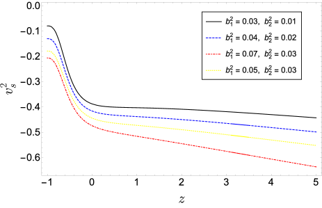
Figure 9: The evolution of $v_{s}^{2}$ versus $z$ for different values of $b_{1}^{2}$ and $b_{2}^{2}$. We set $\Delta=0.5$ and $\Omega_{D}^{0}=0.73$ as initial condition.

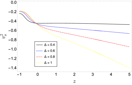
Figure 10: The evolution of $v_{s}^{2}$ versus $z$ for different values of $\Delta$. We set $b_{1}^{2}=0.05$, $b_{2}^{2}=0.04$ and $\Omega_{D}^{0}=0.73$ as initial condition.

III Generalized interacting BHDE model including radiation fluid

Let us now extend the above analysis to the more realistic case where also a radiation fluid is present in the Universe. Denoting by $\rho_{r}$ the energy density of the radiation, Eq. (5) must be generalized to

$$H^{2}=\frac{1}{3m_{p}^{2}}\left(\rho_{m}+\rho_{D}+\rho_{r}\right).\\$$ (22)

Assuming the radiation to be decoupled from BHDE and DM, then the conservation equation for such component takes the form

$$\dot{\rho}_{r}+4H\rho_{r}=0\,.$$ (23)

We also introduce the fractional energy density

$$\Omega_{r}=\frac{\rho_{r}}{\rho_{c}}=\Omega_{r0}\left(1+z\right)^{4}\,,$$ (24)

which allows us to rewrite Eq. (22) as

$$\Omega_{m}+\Omega_{D}+\Omega_{r}=1\,.$$ (25)

If we now differentiate Eq. (22) and then insert Eqs. (11), (23) and (25), we are led to

$$\frac{\dot{H}}{H^{2}}=\frac{1}{2}\left[\Omega_{m}+\Omega_{D}\left(1-3\omega_{D}\right)\right]-2\,,$$ (26)

which coincides with Eq. (13) for $\Omega_{r}=0$, as expected.

In turn, the EoS parameter (14) becomes

$$\omega_{D}=\frac{-\frac{\Delta}{2}+3\left(1-\frac{\Delta}{2}\right)\Omega_{r}}{\left[1+\frac{\Omega_{D}}{2}\left(\Delta-2\right)\right]}\,+\,\frac{\left(b_{1}^{2}-b_{2}^{2}\right)\Omega_{D}+b_{1}^{2}\left(\Omega_{r}-1\right)}{\Omega_{D}\left[1+\frac{\Omega_{D}}{2}\left(\Delta-2\right)\right]}\,,$$ (27)

which gives the following generalized differential equation for $\Omega_{D}$

$$\Omega^{\prime}_{D}=\frac{3\Delta\Omega_{D}}{2}\left[\frac{4-3\Omega_{m}-4\Omega_{D}-b_{1}^{2}\Omega_{m}-b_{2}^{2}\Omega_{D}}{1-\left(1-\frac{\Delta}{2}\right)\Omega_{D}}\right].$$ (28)

By use of Eq. (25), it is easy to show that this expression matches with Eq. (15) in the absence of radiation fluid.

As done in Sec. II, we can solve Eq. (28) numerically (see also Appendix). The behavior of the fractional energy density parameters $\Omega_{D}$, $\Omega_{m}$ and $\Omega_{r}$ is plotted in Fig. 12 for given values of $b_{1}^{2}$, $b_{2}^{2}$ and $\Delta$. It is evident that our model well describes the usual thermal history of the Universe, evolving from an initial radiation dominated era to a matter dominated one. Finally, the Universe enters the DE dominated epoch at $0.52\leq z_{t}\leq 0.82$ (Fig. 16) and $0.52\leq z_{t}\leq 0.97$ (Fig. 16) for the considered values of model parameters. These intervals are again consistent with the observational predictions of Rapetti ; Farooq ; MamonEPJC ; MamonEPJC2 .

On the other hand, in Fig. 12 we plot the evolution of $\Omega_{D}$ in the presence (dashed lines) and absence (solid lines) of radiation fluid for different values of $\Delta$. As expected, the discrepancy between the two sets of curves becomes more evident at higher redshift, where the effects of radiation are more relevant (see Fig. 12). Interestingly enough, we also notice that the larger the value of $\Delta$, the lower the magnitude of the difference between the two sets of curves. This is due to the fact that, for higher $\Delta$, the contribution of BHDE density increases at the expense of the radiation term, whose effects then become increasingly negligible. A similar result has been exhibited in Mamon:2020wnh for the case of the interacting Tsallis Holographic Dark Energy.

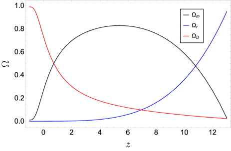
Figure 11: The evolution of $\Omega_{D}$, $\Omega_{m}$ and $\Omega_{r}$ versus $z$. We set $\Delta=0.8$, $b_{1}^{2}=0.03$, $b_{2}^{2}=0.01$ and $\Omega_{D}^{0}=0.73$, $\Omega_{r}^{0}=2.47\times 10^{-5}$ as initial conditions.

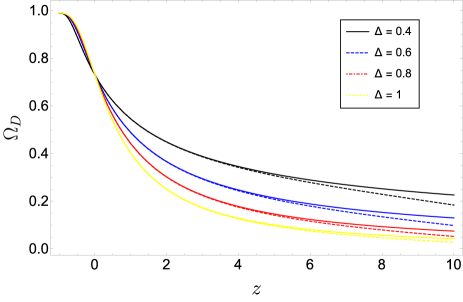
Figure 12: The evolution of $\Omega_{D}$ versus $z$ for different values of $\Delta$. We set $b_{1}^{2}=0.03$, $b_{2}^{2}=0.01$ and $\Omega_{D}^{0}=0.73$, $\Omega_{r}^{0}=2.47\times 10^{-5}$ as initial conditions. The dashed (solid) lines represent the evolution when radiation is present (absent).

The behavior of the BHDE EoS parameter (27) is presented in Fig. 14 for different values of the interaction terms $b_{1}^{2}$ and $b_{2}^{2}$. Again, for lower redshift the dashed and solid lines nearly coincide, which explains why the prediction for the present value of $\omega_{D}$ is the same as that found in the previous Section. In particular, in the interval where the transition from the decelerated to accelerated phase occurs, i.e. $0.5<z_{t}<1$, BHDE lies in the quintessence dominated phase, while it evolves toward a phantom-like behavior for $z\rightarrow-1$. However, as $z$ increases, the two sets of curves depart from each other, in line with the previous discussion. The same profile is exhibited for different values of $\Delta$ (see Fig. 14).

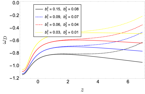
Figure 13: The evolution of $\omega_{D}$ versus $z$ for different values of $b_{1}^{2}$ and $b_{2}^{2}$. We set $\Delta=0.5$ and $\Omega_{D}^{0}=0.73$, $\Omega_{r}^{0}=2.47\times 10^{-5}$ as initial conditions. The dashed (solid) lines represent the evolution when radiation is present (absent).

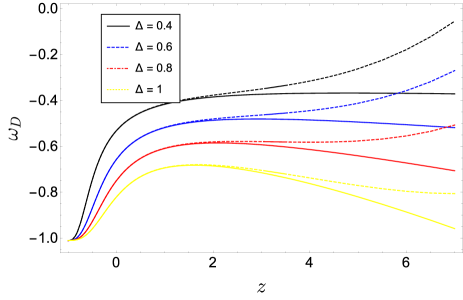
Figure 14: The evolution of $\omega_{D}$ versus $z$ for different values of $\Delta$. We set $b_{1}^{2}=0.03$, $b_{2}^{2}=0.01$ and $\Omega_{D}^{0}=0.73$, $\Omega_{r}^{0}=2.47\times 10^{-5}$ as initial conditions. The dashed (solid) lines represent the evolution when radiation is present (absent).

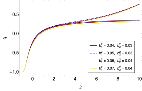
Figure 15: The evolution of $q$ versus $z$ for different values of $b_{1}^{2}$ and $b_{2}^{2}$. We set $\Delta=0.5$ and $\Omega_{D}^{0}=0.73$, $\Omega_{r}^{0}=2.47\times 10^{-5}$ as initial conditions. The dashed (solid) lines represent the evolution when radiation is present (absent).

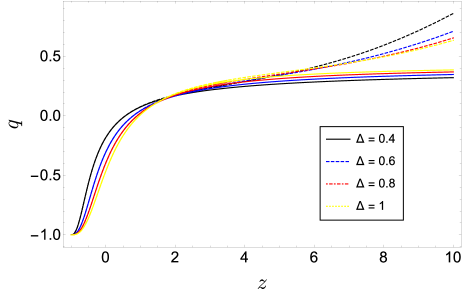
Figure 16: The evolution of $q$ versus $z$ for different values of $\Delta$. We set $b_{1}^{2}=0.05$, $b_{2}^{2}=0.04$ and $\Omega_{D}^{0}=0.73$, $\Omega_{r}^{0}=2.47\times 10^{-5}$ as initial conditions. The dashed (solid) lines represent the evolution when radiation is present (absent).

In Fig. 16 and Fig. 16 we plot the deceleration parameter

$$q=\frac{1}{2}\left\{1+\Omega_{r}^{0}\left(1+z\right)^{4}\,+\,\frac{3\left[-\left(2b_{2}^{2}+\Delta\right)\Omega_{D}-3\Omega_{r}^{0}\left(\Delta-2\right)\left(1+z\right)^{4}\Omega_{D}\right]+6b_{1}^{2}\left[-1+\Omega_{D}+\Omega_{r}^{0}\left(1+z\right)^{4}\right]}{2+\left(\Delta-2\right)\Omega_{D}}\right\}$$ (29)

versus $z$ for different values of $b_{1}^{2},b_{2}^{2}$ and $\Delta$, respectively. We see that also in the present model the Universe evolves from an early decelerated regime (for $z>z_{t}$) to a late accelerated phase (for $z<z_{t}$). The value of $z_{t}$ strongly depends on Barrow parameter $\Delta$, with $z_{t}$ increasing for increasing $\Delta$ (see Fig. 17). However, for $\Delta\gtrsim 0.55$ and the selected values of $b_{1}^{2}$ and $b_{2}^{2}$, we find that $z_{t}>1$, in contrast with the results of Rapetti ; Farooq ; MamonEPJC ; MamonEPJC2 . Thus, large values of $\Delta$ turn out to be disfavored by our model. This is consistent with the stringent upper bounds on $\Delta$ obtained through different cosmological analysis in Anagnostopoulos:2020ctz ; Leon:2021wyx ; Barrow:2020kug ; Jusufi:2021fek ; Dabrowski:2020atl ; Saridakis:2020cqq ; Luciano:2022pzg ; Vagnozzi:2022moj .

Figure 19 and Fig. 19 show the behavior of the jerk parameter

$$j = \frac{1}{2}\,\Bigg{\{}4\Omega_{r}^{0}\left(1+z\right)^{4}-\frac{9\Delta\left(\Delta-2\right)\left[1-b_{1}^{2}+\left(b_{1}^{2}-b_{2}^{2}-1\right)\Omega_{D}+\Omega_{r}^{0}\left(3+b_{1}^{2}\right)\left(1+z\right)^{4}\right]\Omega_{D}}{\left[2+\left(\Delta-2\right)\Omega_{D}\right]^{3}}$$ (30)

$$\times\left\{2b_{1}^{2}+\left(2b_{2}^{2}-2b_{1}^{2}+\Delta\right)\Omega_{D}-\Omega_{r}^{0}\left(1+z\right)^{4}\left[2b_{1}^{2}-3\left(\Delta-2\right)\Omega_{D}\right]\right\}+\frac{3}{2+\left(\Delta-2\right)\Omega_{D}}$$

$$\times\,\Big{\{}8b_{1}^{2}\Omega_{r}^{0}\left(1+z\right)^{4}-12\Omega_{r}^{0}\left(\Delta-2\right)\left(1+z\right)^{4}\Omega_{D}-\frac{6\Delta\left(b_{1}^{2}-b_{2}^{2}\right)\left[1-b_{1}^{2}+\left(b_{1}^{2}-b_{2}^{2}-1\right)\Omega_{D}+\Omega_{r}^{0}\left(3+b_{1}^{2}\right)\left(1+z\right)^{4}\right]\Omega_{D}}{2+\left(\Delta-2\right)\Omega_{D}}$$

$$+\,\frac{3\Delta\left[1-b_{1}^{2}+\left(b_{1}^{2}-b_{2}^{2}-1\right)\Omega_{D}+\Omega_{r}^{0}\left(3+b_{1}^{2}\right)\left(1+z\right)^{4}\right]\left[\Delta+3\Omega_{r}^{0}\left(\Delta-2\right)\left(1+z\right)^{4}\right]\Omega_{D}}{2+\left(\Delta-2\right)\Omega_{D}}\Big{\}}$$

$$+\,\Big{\{}1+\Omega_{r}^{0}\left(1+z\right)^{4}+\frac{3\big{\{}-\left(2b_{2}^{2}+\Delta\right)\Omega_{D}-3\Omega_{r}^{0}\left(\Delta-2\right)\left(1+z\right)^{4}\Omega_{D}+2b_{1}^{2}\left[-1+\Omega_{D}+\Omega_{r}^{0}\left(1+z\right)^{4}\right]\big{\}}}{2+\left(\Delta-2\right)\Omega_{D}}\Big{\}}$$

$$\times\,\Big{\{}2+\Omega_{r}^{0}\left(1+z\right)^{4}+\frac{3\big{\{}-\left(2b_{2}^{2}+\Delta\right)\Omega_{D}-3\Omega_{r}^{0}\left(\Delta-2\right)\left(1+z\right)^{4}\Omega_{D}+2b_{1}^{2}\left[-1+\Omega_{D}+\Omega_{r}^{0}\left(1+z\right)^{4}\right]\big{\}}}{2+\left(\Delta-2\right)\Omega_{D}}\Big{\}}\Bigg{\}}$$

versus the redshift $z$. As in the absence of radiation, we find that $j>0$ and tends to unity in the far future (i.e. $z\rightarrow-1$). Once more, the discrepancy between the curves representing the evolution of $j$ with (dashed lines) and without (solid lines) radiation becomes greater for higher redshift, where the contribution of radiation dominates.

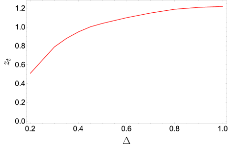
Figure 17: Transition redshift $z_{t}$ versus $\Delta$. We set $b_{1}^{2}=0.07$, $b_{2}^{2}=0.06$ and $\Omega_{D}^{0}=0.73$, $\Omega_{r}^{0}=2.47\times 10^{-5}$ as initial conditions.

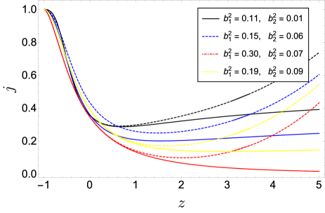
Figure 18: The evolution of $j$ versus $z$ for different values of $b_{1}^{2}$ and $b_{2}^{2}$. We set $\Delta=0.5$ and $\Omega_{D}^{0}=0.73$, $\Omega_{r}^{0}=2.47\times 10^{-5}$ as initial conditions. The dashed (solid) lines represent the evolution when radiation is present (absent).

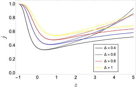
Figure 19: The evolution of $j$ versus $z$ for different values of $\Delta$. We set $b_{1}^{2}=0.05$, $b_{2}^{2}=0.04$ and $\Omega_{D}^{0}=0.73$, $\Omega_{r}^{0}=2.47\times 10^{-5}$ as initial conditions. The dashed (solid) lines represent the evolution when radiation is present (absent).

To conclude, in Fig. 21 and Fig. 21 we plot the evolution of the square of sound speed

$$v_{s}^{2} = \frac{1}{\Omega_{D}\left[2+\left(\Delta-2\right)\Omega_{D}\right]^{2}}\Bigg{\{}2\left[2+\left(\Delta-2\right)\Omega_{D}\right]\Big{\{}\left(b_{1}^{2}-b_{2}^{2}\right)\Omega_{D}+b_{1}^{2}\left[-1+\Omega_{r}^{0}\left(1+z\right)^{4}\right]$$ (31)

$$+\left[-\frac{\Delta}{2}-\frac{3}{2}\Omega_{r}^{0}\left(\Delta-2\right)\left(1+z\right)^{4}\right]\Omega_{D}\Big{\}}+\frac{\Delta}{\Delta-2}\Big{\{}-2b_{1}^{2}\big{\{}\left(\Delta-2\right)\Omega_{D}^{2}+2\left[-1+\Omega_{r}^{0}\left(1+z\right)^{4}\right]$$

$$\,+2\left(\Delta-2\right)\left[-1+\Omega_{r}^{0}\left(1+z\right)^{4}\right]\Omega_{D}\big{\}}+\left(\Delta-2\right)\big{\{}2b_{2}^{2}-6\Omega_{r}^{0}\left(1+z\right)^{4}+\Delta\left[1+3\Omega_{r}^{0}\left(1+z\right)^{4}\right]\big{\}}\Omega_{D}^{2}\Big{\}}\Bigg{\}}$$

against redshift for different values of $b_{1}^{2}$, $b_{2}^{2}$ and $\Delta$, respectively. It is interesting to note that, when the effects of radiation are considered, the model is classically stable ($v_{s}^{2}>0$) at early times (higher redshifts), while it becomes unstable at later times (lower redshifts). This feature is peculiar to the generalized interacting BHDE model considered in this section.

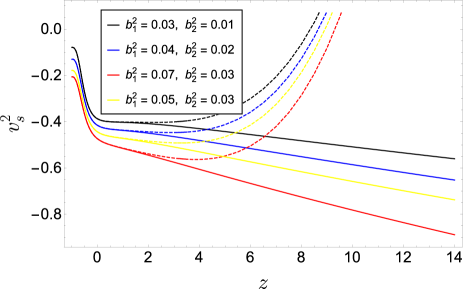
Figure 20: The evolution of $v_{s}^{2}$ versus $z$ for different values of $b_{1}^{2}$ and $b_{2}^{2}$. We set $\Delta=0.5$ and $\Omega_{D}^{0}=0.73$, $\Omega_{r}^{0}=2.47\times 10^{-5}$ as initial conditions. The dashed (solid) lines represent the evolution when radiation is present (absent).

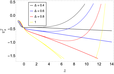
Figure 21: The evolution of $v_{s}^{2}$ versus $z$ for different values of $\Delta$. We set $b_{1}^{2}=0.05$, $b_{2}^{2}=0.04$ and $\Omega_{D}^{0}=0.73$, $\Omega_{r}^{0}=2.47\times 10^{-5}$ as initial conditions. The dashed (solid) lines represent the evolution when radiation is present (absent).

IV Thermodynamics of generalized interacting BHDE model

Let us now study the thermodynamic implications of the present model. We stress that our analysis extends that of Mamon:2020wnh to the case where also radiation is included in the energy budget of the Universe. We consider the Universe as a thermodynamic system bounded by the cosmological apparent horizon of radius Bak

$$r_{h}=\left(H^{2}+\frac{k}{a^{2}}\right)^{-1/2}\,,$$ (32)

where $k$ is the spatial curvature. Clearly, for a spatially flat Universe, the above equation gives $r_{h}=1/H$.

Denoting by $S_{D}$, $S_{m}$ and $S_{r}$ the entropies of BHDE, DM and radiation, respectively, and by $S_{f}=S_{D}+S_{m}+S_{r}$ their sum, the total entropy $S_{tot}$ of the Universe is

$$S_{tot}=S_{f}+S_{h}\,,$$ (33)

where $S_{h}$ is the horizon entropy.

If we consider the Universe as an isolated system, then according to the generalized second law (GSL) of thermodynamics $S$ should obey the inequality Mamon:2020wnh ; Mamon:2020spa

$$\dot{S}_{tot}\geq 0\,.$$ (34)

As noted in Mamon:2020wnh , this condition should hold throughout the evolution of the Universe.

In order to establish whether the GSL is satisfied, let us remember that the horizon entropy $S_{h}$ in BHDE is given by Eq. (1), here rewritten as

$$S_{h}=\gamma r_{h}^{\Delta+2}\,,$$ (35)

where we have expressed the horizon area as $A=4\pi r_{h}^{2}$ and $\gamma=(4\pi/A_{0})^{1+\Delta/2}>0$.

Furthermore, the temperature of the apparent horizon is

$$T=\frac{1}{2\pi r_{h}}\,,$$ (36)

which is formally analogous to the temperature associated to the event horizon of a black hole with the same radius $r_{h}$ CaiKim . At this stage, it is worth noting that such temperature is typically assumed equal to the temperature of the composite matter inside the horizon, otherwise a temperature gradient might arise. In turn, the ensuing energy flow would imply a deformation of the horizon geometry and the need to resort to non-equilibrium thermodynamics Izquierdo ; Padmanabhan:2009vy ; Jamil1 ; Jamil2 ; Mimoso .

Now, the first law of thermodynamics for BHDE, DM and radiation takes the form

$$T\,dS_{D}=dE_{D}+p_{D}\,dV\,,\qquad T\,dS_{m}=dE_{m}\,,\qquad T\,dS_{r}=dE_{r}+p_{r}\,dV\,,$$ (37)

where $V=4\pi r_{h}^{3}/3$ is the spherical volume occupied by the fluid inside the horizon and we have taken into account the assumption of pressureless dark matter (i.e. $p_{m}=0$). Moreover, $E_{D}=4\pi r_{h}^{3}\rho_{D}/3$, $E_{m}=4\pi r_{h}^{3}\rho_{m}/3$ and $E_{r}=4\pi r_{h}^{3}\rho_{r}/3$ denote the internal energies of BHDE, DM and radiation, respectively, while $p_{r}=\rho_{r}/3$ is the radiation pressure.

Differentiation of Eqs. (35) and (37) respect to time gives

$$\dot{S}_{h}=\left(\Delta+2\right)\gamma\,r_{h}^{\Delta+1}\dot{r}_{h}\,,$$ (38)

and

$$\dot{S}_{D}=\frac{1}{T}\left(\dot{E}_{D}+4\pi\,p_{D}\hskip 1.42262ptr^{2}_{h}\hskip 1.42262pt\dot{r}_{h}\right),\qquad\dot{S}_{r}=\frac{\dot{E}_{m}}{T}\,,\qquad\dot{S}_{r}=\frac{1}{T}\left(\dot{E}_{r}+4\pi\,p_{r}\hskip 1.42262ptr^{2}_{h}\hskip 1.42262pt\dot{r}_{h}\right).$$ (39)

Identifying the temperature $T$ in Eq. (39) with the horizon temperature (36), the total entropy variation of the thermodynamic system bounded by the dynamical apparent horizon is

$$\dot{S}_{tot}=\frac{2\pi}{G}\frac{\dot{H}}{H^{5}}\left[\dot{H}+H^{2}-\frac{\gamma G\left(\Delta+2\right)}{2\pi}H^{2-\Delta}\right]\,.$$ (40)

Notice that, for $\Delta=0$, the above expression reproduces the usual BH entropy variation $\dot{S}_{tot}=\frac{2\pi}{G}\frac{\dot{H}^{2}}{H^{5}}$, which takes non-negative values for any $H$. This entails the validity of the GSL of thermodynamics at any time within the standard framework. On the other hand, for $\Delta\neq 0$, we infer that $\dot{S}_{tot}\geq 0$, provided that

$$\dot{H}>0\,\,\,\,\,\mathrm{and}\,\,\,\,\,\left[\dot{H}+H^{2}-\frac{\gamma G\left(\Delta+2\right)}{2\pi}H^{2-\Delta}\right]\geq 0\,,$$ (41)

or

$$\dot{H}<0\,\,\,\,\,\mathrm{and}\,\,\,\,\,\left[\dot{H}+H^{2}-\frac{\gamma G\left(\Delta+2\right)}{2\pi}H^{2-\Delta}\right]\leq 0\,.$$ (42)

Therefore, we find that in our model the total entropy variation is not necessarily a non-negative function, potentially yielding a violation of the GSL of thermodynamics. A similar result is exhibited in the case of interacting Tsallis Holographic Dark Energy Mamon:2020wnh and BHDE in the absence of fluid radiation Mamon:2020spa . A deeper understanding of this result requires further study that will be presented elsewhere.

V Conclusions and outlook

We have analyzed a generalized interacting HDE model with Barrow entropy, which is based on a modified horizon endowed with a fractal structure due to quantum gravitational corrections BarrowBH . Within this framework, we have studied the evolution of a spatially flat FLRW Universe filled by pressureless dark matter, radiation fluid and BHDE, whose IR cutoff is set equal to the Hubble length. We have assumed a suitable interaction between the dark sectors of the cosmos, which reproduces well-known interactions in the literature for some specific values of the model parameters Mamon:2020wnh . The behavior of various quantities, such as the BHDE density parameter, the equation of state parameter, the deceleration parameter, the jerk parameter and the square of sound speed has been investigated. As a result, we have found that the present model well describes the thermal history of the Universe, with the sequence of radiation, dark matter and dark energy epochs, before resulting in a complete dark energy domination in the far future. Moreover, the cosmic evolution of the Universe is nontrivially affected by both the interaction terms $b_{1}^{2},b_{2}^{2}$ and Barrow parameter $\Delta$. Concerning the jerk parameter, we have shown that $j>0$ and approaches to the $\Lambda$CDM model value $j=1$ as $z\rightarrow-1$. Finally, we have calculated the square of sound speed to examine the classical stability of our model against small perturbations. While in the absence of radiation the interacting BHDE model is always unstable ($v_{s}^{2}<0$), it becomes classically stable ($v_{s}^{2}>0$) at early times when the effects or radiation are taken into account. Results are summarized in Table 1, from which we infer the constraints $0.03\leq b_{1}^{2}\leq 0.15$, $0.01\leq b_{2}^{2}\leq 0.08$ and $\Delta<0.55$ to allow consistency with observations. We notice that while the bound on Barrow parameter is slightly wider than those obtained in so-far literature Anagnostopoulos:2020ctz ; Leon:2021wyx ; Barrow:2020kug ; Jusufi:2021fek ; Dabrowski:2020atl ; Saridakis:2020cqq ; Luciano:2022pzg ; Vagnozzi:2022moj ; DiGennaro:2022ykp , constraints on the interaction terms are well-consistent or improve past results (see for instance Newp ; Telep ).

Without radiation	With radiation
Quintessence/Cosmological constant ($z>-1$)	Quintessence/Cosmological constant ($z>-1$)
Phantom ($z\rightarrow-1$)	Phantom ($z\rightarrow-1$)
$-0.9\leq\omega_{D_{0}}\leq-0.64$ ($0.03\leq b_{1}^{2}\leq 0.15,0.01\leq b_{2}^{2}\leq 0.08,\Delta=0.5$)	$-0.9\leq\omega_{D_{0}}\leq-0.64$ ($0.03\leq b_{1}^{2}\leq 0.15,0.01\leq b_{2}^{2}\leq 0.08,\Delta=0.5$)
$0.56\leq z_{t}\leq 0.83$ ($0.04\leq b_{1}^{2}\leq 0.07,0.03\leq b_{2}^{2}\leq 0.04,\Delta=0.5$)	$0.52\leq z_{t}\leq 0.82$ ($0.04\leq b_{1}^{2}\leq 0.07,0.03\leq b_{2}^{2}\leq 0.04,\Delta=0.5$)
$-0.46\leq q_{0}\leq-0.17$ ($b_{1}^{2}=0.05,b_{2}^{2}=0.04,0.4\leq\Delta\leq 1$)	$-0.46\leq q_{0}\leq-0.17$ ($b_{1}^{2}=0.05,b_{2}^{2}=0.04,0.4\leq\Delta\leq 1$)
$j>0$ (for all $z$), $j(z\rightarrow-1)\rightarrow 1$	$j>0$ (for all $z$), $j(z\rightarrow-1)\rightarrow 1$
$v_{s}^{2}<0$ (for all $z$)	$v_{s}^{2}>0$ ($z\gg 1$), $v_{s}^{2}<0$ ($z\rightarrow-1$)

Table 1: Theoretical predictions of EoS parameter, transition redshift, deceleration parameter, jerk parameter and square of sound speed (for the current values of these quantities, we only report the best prediction of our models according to recent observations. Notice that such values are nearly equal for the two models, since effects of radiation fluid are only relevant at early times $z\gg 1$).

As a further study, we have investigated the implications of gravity-thermodynamics in the BHDE model by assuming the apparent horizon as cosmological boundary. We have found that, while in the standard HDE based on BH entropy ($\Delta=0$) the GSL of thermodynamics is always satisfied, on the other hand it might be violated in BHDE ($\Delta\neq 0$), depending on the evolution of the Universe.

Several aspects remain to be addressed. For instance, it would be interesting to investigate the properties of BHDE by considering different IR cutoffs and/or interactions between DM and DE. On the other hand, one might think of extending the present analysis to the case of HDE based on Kaniadakis entropy, which is a self-consistent extension of Boltzmann-Gibbs entropy that arises from relativistic statistical theory Kana . In this case, deviations from the standard framework are characterized by the parameter $-1<K<1$. Along this line, a challenging perspective is to search for any correspondence between the two generalizations of HDE and possible relations between Barrow and Kaniadakis parameters. Finally, since our model provides a phenomenological attempt to account for quantum gravity effects in the evolution of the Universe via the introduction of Barrow entropy, it is important to analyze whether our predictions reconcile with more fundamental candidate theories or phenomenological model of quantum gravity. In this sense, preliminary attempts to establish a connection between deformed entropies and generalizations of the Heisenberg principle induced by quantum gravitational effects have been proposed in Shababi ; LucGUP ; JizbaGUP . Work along these directions is in progress and is reserved for future publications.

Appendix A Dark energy evolution

In order to infer some more detail on the solution of Eq. (15), we express such equation as a differential system in the plane of the form

$$\frac{d\Omega_{D}}{dz}\,=\,3\Delta\Omega_{D}\left[1-\Omega_{D}-b_{1}^{2}+(b_{1}^{2}-b_{2}^{2})\Omega_{D}\right]\,,\qquad\frac{da}{dz}\,=\,2-(2-\Delta)\Omega_{D}\,.$$ (43)

A first integral associated to this system is now

$$I\,=\,a^{-3\Delta}\Omega_{D}^{-\frac{2}{b_{1}^{2}-1}}\left[1-b_{1}^{2}-\Omega_{D}+(b_{1}^{2}-b_{2}^{2})\Omega_{D}\right]^{\frac{(b_{1}^{2}-1)\Delta-2b_{2}^{2}}{(b_{1}^{2}-1)(b_{1}^{2}-b_{2}^{2}-1)}}\,,$$ (44)

and any solution of Eq. (15) is given by setting $I=C$, where $C$ is an arbitrary constant. Specifically, in our case this constant can be fixed by imposing the condition $\Omega_{D}^{0}=0.73$.

For Eq. (28) we cannot proceed as above, since we are now in presence of an ordinary differential equation depending on two variables $\Omega_{D}$ and $\Omega_{m}$. However, we can consider the two following different regimes:

• $z\gg 1$ and $z\rightarrow-1$, where we can roughly consider $\Omega_{m}\simeq 0$ (see Fig. 12). In this case the differential system associated to Eq. (28) is

  $$\frac{d\Omega_{D}}{dz}=3\Delta\Omega_{D}(4-4\Omega_{D}-b_{2}^{2}\Omega_{D}),\quad\frac{da}{dz}=2-(2-\Delta)\Omega_{D}\,.$$ (45)

  A first integral associated to this differential system is then

  $$I=a^{3\Delta}\Omega_{D}^{-\frac{1}{2}}\left[(4+b_{2}^{2})\Omega_{D}-4\right]^{\frac{b_{2}^{2}+2\Delta}{2b_{2}^{2}+8}}.$$

• On the other hand, we can specialize Eq. (28) to the present time $z=0$, where we know that $\Omega^{0}_{m}/\Omega^{0}_{D}\simeq 1/3$. Substitution into Eq. (28) then gives the differential system

  $$\frac{d\Omega_{D}}{d\tau}\,=\,3\Delta\Omega_{D}(4-5\Omega_{D}-b_{1}^{2}\Omega_{D}/3-b_{2}^{2}\Omega_{D}),\quad\frac{da}{d\tau}\,=\,2-(2-\Delta)\Omega_{D},$$ (46)

  and the first integral associated to this system is

  $$I=a^{\Delta}\Omega_{D}^{-\frac{1}{6}}\{\left[b_{1}^{2}+3(5+b_{2}^{2})\right]\Omega_{D}\}^{\frac{1}{6}+\frac{\Delta-2}{b_{1}^{2}+3(5+b_{2}^{2})}}.$$ (47)

References

- (1) A. G. Riess et al. [Supernova Search Team], Astron. J. 116, 1009 (1998).
- (2) S. Perlmutter et al. [Supernova Cosmology Project], Astrophys. J. 517, 565 (1999).
- (3) D. N. Spergel et al. [WMAP], Astrophys. J. Suppl. 148, 175 (2003).
- (4) M. Tegmark et al. [SDSS], Phys. Rev. D 69, 103501 (2004).
- (5) P. A. R. Ade et al. [Planck], Astron. Astrophys. 571, A16 (2014).
- (6) P. J. E. Peebles and B. Ratra, Astrophys. J. Lett. 325, L17 (1988).
- (7) B. Ratra and P. J. E. Peebles, Phys. Rev. D 37, 3406 (1988).
- (8) C. Wetterich, Nucl. Phys. B 302, 668 (1988).
- (9) J. A. Frieman, C. T. Hill, A. Stebbins and I. Waga, Phys. Rev. Lett. 75, 2077 (1995).
- (10) M. S. Turner and M. J. White, Phys. Rev. D 56, R4439 (1997).
- (11) R. R. Caldwell, R. Dave and P. J. Steinhardt, Phys. Rev. Lett. 80, 1582 (1998).
- (12) C. Armendariz-Picon, V. F. Mukhanov and P. J. Steinhardt, Phys. Rev. Lett. 85, 4438 (2000).
- (13) L. Amendola, Phys. Rev. D 62, 043511 (2000).
- (14) C. Armendariz-Picon, V. F. Mukhanov and P. J. Steinhardt, Phys. Rev. D 63, 103510 (2001).
- (15) A. Y. Kamenshchik, U. Moschella and V. Pasquier, Phys. Lett. B 511, 265 (2001).
- (16) R. R. Caldwell, Phys. Lett. B 545, 23 (2002).
- (17) R. R. Caldwell, M. Kamionkowski and N. N. Weinberg, Phys. Rev. Lett. 91, 071301 (2003)
- (18) S. Nojiri and S. D. Odintsov, Phys. Lett. B 562, 147 (2003).
- (19) B. Feng, X. L. Wang and X. M. Zhang, Phys. Lett. B 607, 35 (2005).
- (20) Z. K. Guo, Y. S. Piao, X. M. Zhang and Y. Z. Zhang, Phys. Lett. B 608, 177 (2005).
- (21) E. Elizalde, S. Nojiri and S. D. Odintsov, Phys. Rev. D 70, 043539 (2004).
- (22) S. Nojiri, S. D. Odintsov and S. Tsujikawa, Phys. Rev. D 71, 063004 (2005).
- (23) C. Deffayet, G. R. Dvali and G. Gabadadze, Phys. Rev. D 65, 044023 (2002).
- (24) A. Sen, JHEP 07, 065 (2002).
- (25) Z. Zhang, Class. Quant. Grav. 39, 015003 (2022).
- (26) A. G. Cohen, D. B. Kaplan and A. E. Nelson, Phys. Rev. Lett. 82, 4971 (1999).
- (27) P. Horava and D. Minic, Phys. Rev. Lett. 85, 1610 (2000).
- (28) S. D. Thomas, Phys. Rev. Lett. 89, 081301 (2002).
- (29) M. Li, Phys. Lett. B 603, 1 (2004).
- (30) S. D. H. Hsu, Phys. Lett. B 594, 13 (2004).
- (31) Q. G. Huang and M. Li, JCAP 08, 013 (2004).
- (32) B. Wang, C. Y. Lin and E. Abdalla, Phys. Lett. B 637, 357 (2006).
- (33) M. R. Setare, Phys. Lett. B 642, 421 (2006).
- (34) L.N. Granda, A. Oliveros, Phys. Lett. B 671275, 199 (2009).
- (35) A. Sheykhi, Phys. Rev. D 84, 107302 (2011).
- (36) K. Bamba, S. Capozziello, S. Nojiri and S. D. Odintsov, Astrophys. Space Sci. 342, 155 (2012).
- (37) S. Ghaffari, M. H. Dehghani and A. Sheykhi, Phys. Rev. D 89, 123009 (2014).
- (38) S. Wang, Y. Wang and M. Li, Phys. Rept. 696, 1 (2017).
- (39) H. Moradpour, A. H. Ziaie and M. Kord Zangeneh, Eur. Phys. J. C 80, 732 (2020).
- (40) J. D. Bekenstein, Phys. Rev. D 7, 2333 (1973).
- (41) K. Enqvist, S. Hannestad and M. S. Sloth, JCAP 02, 004 (2005).
- (42) M. R. Setare, Phys. Lett. B 653, 116 (2007).
- (43) S. Srivastava and U. K. Sharma, Int. J. Geom. Meth. Mod. Phys. 18, 2150014 (2021).
- (44) M. Tavayef, A. Sheykhi, K. Bamba and H. Moradpour, Phys. Lett. B 781, 195 (2018).
- (45) E. N. Saridakis, K. Bamba, R. Myrzakulov and F. K. Anagnostopoulos, JCAP 12, 012 (2018).
- (46) S. Nojiri, S. D. Odintsov and E. N. Saridakis, Eur. Phys. J. C 79, 242 (2019)..
- (47) N. Drepanou, A. Lymperis, E. N. Saridakis and K. Yesmakhanova, Eur. Phys. J. C 82, 449 (2022).
- (48) A. Hernández-Almada, G. Leon, J. Magaña, M. A. García-Aspeitia, V. Motta, E. N. Saridakis and K. Yesmakhanova, Mon. Not. Roy. Astron. Soc. 511, 4147 (2022).
- (49) E. N. Saridakis, Phys. Rev. D 102, 123525 (2020).
- (50) M. P. Dabrowski and V. Salzano, Phys. Rev. D 102, 064047 (2020).
- (51) A. Sheykhi, Phys. Rev. D 103, 123503 (2021).
- (52) P. Adhikary, S. Das, S. Basilakos and E. N. Saridakis, Phys. Rev. D 104, 123519 (2021).
- (53) S. Nojiri, S. D. Odintsov and T. Paul, Phys. Lett. B 825, 136844 (2022).
- (54) G. G. Luciano and J. Gine, Phys. Lett. B 833, 137352 (2022).
- (55) G. G. Luciano, Eur. Phys. J. C 82, 314 (2022).
- (56) G. G. Luciano and Y. Liu, [arXiv:2205.13458 [hep-th]].
- (57) F. K. Anagnostopoulos, S. Basilakos and E. N. Saridakis, Eur. Phys. J. C 80, 826 (2020).
- (58) S. Ghaffari, G. G. Luciano and S. Capozziello, [arXiv:2209.00903 [gr-qc]].
- (59) G. G. Luciano, [arXiv:2210.06320 [gr-qc]].
- (60) A. Arbey and F. Mahmoudi, Prog. Part. Nucl. Phys. 119, 103865 (2021).
- (61) A. Addazi, J. Alvarez-Muniz, R. Alves Batista, G. Amelino-Camelia, V. Antonelli, M. Arzano, M. Asorey, J. L. Atteia, S. Bahamonde and F. Bajardi, et al. Prog. Part. Nucl. Phys. 125, 103948 (2022).
- (62) Y. L. Bolotin, A. Kostenko, O. A. Lemets and D. A. Yerokhin, Int. J. Mod. Phys. D 24, 1530007 (2014).
- (63) L. Amendola and S. Tsujikawa, Dark Energy: Theory and Observations (Cambridge University Press, Cambridge, UK) 2010.
- (64) E. Di Valentino, A. Melchiorri and O. Mena, Phys. Rev. D 96, 043503 (2017).
- (65) S. Kumar and R. C. Nunes, Phys. Rev. D 96, 103511 (2017).
- (66) A. Saha and S. Ghose, Astrophys. Space Sci. 365, 98 (2020).
- (67) S. Ghaffari, H. Moradpour, I. P. Lobo, J. P. Morais Graça and V. B. Bezerra, Eur. Phys. J. C 78, 706 (2018).
- (68) A. Iqbal and A. Jawad, Phys. Dark Univ. 26, 100349 (2019).
- (69) A. A. Mamon, A. H. Ziaie and K. Bamba, Eur. Phys. J. C 80, 974 (2020).
- (70) A. A. Mamon, A. Paliathanasis and S. Saha, Eur. Phys. J. Plus 136, 134 (2021).
- (71) J. D. Barrow, Phys. Lett. B 808, 135643 (2020).
- (72) G. Leon, J. Magaña, A. Hernández-Almada, M. A. García-Aspeitia, T. Verdugo and V. Motta, JCAP 12, 032 (2021).
- (73) K. Jusufi, M. Azreg-Aïnou, M. Jamil and E. N. Saridakis, Universe 8, 2 (2022).
- (74) J. D. Barrow, S. Basilakos and E. N. Saridakis, Phys. Lett. B 815, 136134 (2021).
- (75) E. N. Saridakis and S. Basilakos, Eur. Phys. J. C 81, 644 (2021).
- (76) G. G. Luciano and E. N. Saridakis, Eur. Phys. J. C 82, 558 (2022).
- (77) S. Vagnozzi, R. Roy, Y. D. Tsai and L. Visinelli, [arXiv:2205.07787 [gr-qc]].
- (78) S. Di Gennaro and Y. C. Ong, [arXiv:2205.09311 [gr-qc]].
- (79) L. P. Chimento, A. S. Jakubi, D. Pavon and W. Zimdahl, Phys. Rev. D 67, 083513 (2003).
- (80) D. Pavon and W. Zimdahl, Phys. Lett. B 628, 206 (2005).
- (81) C. G. Boehmer, G. Caldera-Cabral, R. Lazkoz and R. Maartens, Phys. Rev. D 78, 023505 (2008).
- (82) G. Caldera-Cabral, R. Maartens and L. A. Urena-Lopez, Phys. Rev. D 79, 063518 (2009).
- (83) L. P. Chimento, Phys. Rev. D 81, 043525 (2010).
- (84) N. Aghanim et al. [Planck], Astron. Astrophys. 641, A6 (2020) [erratum: Astron. Astrophys. 652, C4 (2021)].
- (85) D. Rapetti, S. W. Allen, M. A. Amin and R. D. Blandford, Mon. Not. Roy. Astron. Soc. 375, 1510 (2007).
- (86) O. Farooq, F. R. Madiyar, S. Crandall and B. Ratra, Astrophys. J. 835, 26 (2017).
- (87) A. A. Mamon and S. Das, Eur. Phys. J. C 77, 495 (2017).
- (88) A. A. Mamon, K. Bamba and S. Das, Eur. Phys. J. C 77, 29 (2017).
- (89) Z. Li, P. Wu and H. Yu, Phys. Lett. B 695, 1 (2011).
- (90) R. D. Blandford, M. A. Amin, E. A. Baltz, K. Mandel and P. J. Marshall, ASP Conf. Ser. 339, 27 (2005).
- (91) D. Bak and S. J. Rey, Class. Quant. Grav. 17, L83 (2000).
- (92) R. G. Cai and S. P. Kim, JHEP 02, 050 (2005).
- (93) G. Izquierdo and D. Pavon, Phys. Lett. B 633, 420 (2006).
- (94) T. Padmanabhan, Rept. Prog. Phys. 73, 046901 (2010).
- (95) M. Jamil, E. N. Saridakis and M. R. Setare, JCAP 11, 032 (2010).
- (96) M. Jamil, E. N. Saridakis and M. R. Setare, Phys. Rev. D 81, 023007 (2010).
- (97) N. K. P and T. K. Mathew, [arXiv:2112.07310 [gr-qc]].
- (98) M. Koussour, S. H. Shekh and M. Bennai, [arXiv:2203.08181 [gr-qc]].
- (99) J. P. Mimoso and D. Pavón, Phys. Rev. D 94, 103507 (2016).
- (100) G. Kaniadakis, Phys. Rev. E 66, 056125 (2002).
- (101) H. Shababi and K. Ourabah, Eur. Phys. J. Plus 135, 697 (2020).
- (102) G. G. Luciano, Eur. Phys. J. C 81, 672 (2021).
- (103) P. Jizba, G. Lambiase, G. G. Luciano and L. Petruzziello, Phys. Rev. D 105, L121501 (2022).