Simultaneous Translation for Unsegmented Input:
A Sliding Window Approach

Abstract

In the cascaded approach to spoken language translation (SLT), the ASR output is typically punctuated and segmented into sentences before being passed to MT, since the latter is typically trained on written text. However, erroneous segmentation, due to poor sentence-final punctuation by the ASR system, leads to degradation in translation quality, especially in the simultaneous (online) setting where the input is continuously updated. SSAlso, in the inference time, we are using online text-flow which means we are not handling unstable input. I am not sure how do I rephrase the last sentence without a risk. For now I am keeping as it is for the submission purpose. To reduce the influence of automatic segmentation, we present a sliding window approach to translate raw ASR outputs (online or offline) without needing to rely on an automatic segmenter. We train translation models using parallel windows (instead of parallel sentences) extracted from the original training data. At test time, we translate at the window level and join the translated windows using a simple approach to generate the final translation. Experiments on English-to-German and English-to-Czech show that our approach improves 1.3–2.0 BLEU points over the usual ASR-segmenter pipeline, and the fixed-length window considerably reduces flicker compared to a baseline retranslation-based online SLT system.

Simultaneous Translation for Unsegmented Input:
A Sliding Window Approach

Sukanta Sen University of Edinburgh sukantasen10@gmail.com                        Ondřej Bojar Charles University MFF ÚFAL bojar@ufal.mff.cuni.cz                        Barry Haddow University of Edinburgh bhaddow@ed.ac.uk

1 Introduction

For machine translation (MT) with textual input, it is usual to segment the text into sentences before translation, with the boundaries of sentences in most text types indicated by punctuation. For spoken language translation (SLT), in contrast, the input is audio so there is no punctuation provided to assist segmentation. Segmentation thus has to be guessed by the ASR system or a separate component. Perhaps more importantly, for many speech genres the input cannot easily be segmented into well-formed sentences as found in MT training data, giving a mismatch between training and test.

In order to address the segmentation problem in SLT, systems often include a segmentation component in their pipeline, e.g. Cho et al. (2017). In other words, a typical cascaded SLT system consists of automatic speech recognition (ASR – which outputs lowercased, unpunctuated text) a punctuator/segmenter (which adds punctuation and so defines segments) and an MT system. The segmenter can be a sequence-sequence model, and training data is easily synthesised from punctuated text. However adding segmentation as an extra step has the disadvantage of introducing an extra component to be managed and deployed. Furthermore, errors in segmentation have been shown to contribute significantly to overall errors in SLT (Li et al., 2021), since neural MT is known to be susceptible to degradation from noisy input Khayrallah and Koehn (2018).

These issues with segmentation can be exacerbated in the online or simultaneous setting. This is an important use case for SLT where we want to produce the translations from live speech, as the speaker is talking. To minimise the latency of the translation, we would like to start translating before speaker has finished their sentence. Some online low-latency ASR approaches will also revise their output after it has been produced, creating additional difficulties for the downstream components. In this scenario, the segmentation into sentences will be more uncertain and we are faced with the choice of waiting for the input to stabilise (so increasing latency) or translating early (potentially introducing more errors, or having to correct the output when the ASR is extended and updated).

To address the segmentation issue in SLT, Li et al. (2021) has proposed to a data augmentation technique which simulates the bad segmentation in the training data. They concatenate two adjacent source sentences (and also the corresponding targets) and then start and end of the concatenated sentences are truncated proportionally.

We use a sliding window approach to translate unsegmented input. In this approach, we translate the ASR output as a series of overlapping windows, using a merging algorithm to turn the translated windows into a single continuous (but still sometimes updated) stream. The process is illustrated in Figure 1. To generate the training data, we convert the sentence-aligned training data into window-window pairs, and remove punctuation and casing from the source. We explain our algorithms in detail in Section 2.

For online SLT, we use a retranslation approach (Niehues et al., 2016; Arivazhagan et al., 2020a), where the MT system retranslates a recent portion of the input each time there is an update from ASR. This approach has the advantage that it can use standard MT inference, including beam search, and does not require a modified inference engine as in streaming approaches (e.g. Ma et al. (2019)). Retranslation may introduce flicker, i.e. potentially disruptive changes of displayed text, when outputs are updated. Flicker can be traded off with latency by masking the last $k$ words of the output (Arivazhagan et al., 2020a). Our sliding window approach is easily combined with retranslation to create an online SLT system which can operate on unsegmented ASR. Each time there is an update from ASR, we retranslate the last $n$ tokens and merge the latest translation into the output stream. Using the fixed size window has the advantage of reducing flicker, since we control how much of the output stream can change on each retranslation.

Experiments on English$\rightarrow$Czech and English$\rightarrow$German show that our sliding window approach improves BLEU scores for both online and offline SLT. For the online case, our approach improves the tradeoff between latency and flicker.

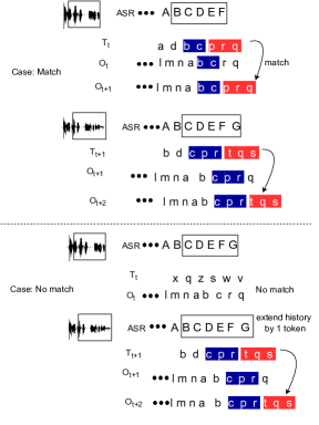
Figure 1: Example of how our proposed window-based translation works at test time in case of a match and no-match of translations of two subsequent windows. The text inside the rectangular box is the source window at time $t$, which is translated into output window (T_t) by the MT system. The text in blue (dark) shade shows the common segment between the output window (T_t) and the output stream (O_t) at time $t$. The text in red shade shows the segment newly added from the output window T_t into the output stream O_t+1. With no common segment between T_t and O_t (“No match”), we extend the input window into the history and translate again. $\bullet\bullet\bullet$ indicates there are more tokens. Note that we used characters here (instead of tokens) just for explanation.

2 Window-Based Translation

2.1 Preprocessing

To make the parallel corpus resemble ASR output, we remove all punctuation (and other special characters) from the source sentences and replace it with spaces. We then remove repeated spaces, and lowercase the source.

2.2 Generating the Window Pairs for Training

To convert the parallel corpus into a set of parallel windows, we use a word-alignment based approach. We first word-align the pre-processed parallel corpus using fast_align (Dyer et al., 2013), then we concatenate each side of the corpus to give two long lines. Note that the word alignments will however never cross sentence boundaries. We randomly select windows of length 15–25 from the target side, and use the word alignment to get the corresponding source window. The algorithms are described in Appendix B.

A subtle detail is whether the original corpus was or was not shuffled at the level of sentences. An original, non-shuffled corpus provides the MT system with useful examples of cross-sentence conditioning, a very useful feature especially for spontaneous speech translation. A minority of our cs-en data is shuffled, which adds some noise to the process, but our method works despite this.

2.3 Translating Input Windows

In our simultaneous MT setting, we assume that the ASR system is transcribing the incoming speech signal into a continuous stream of text. To obtain a new input to the MT system, a fixed-side window is shifted by one token to right every time the stream is extended. For every input window, the MT system translates it and sends it to the module that joins the output windows to the output stream as described in the next section.

2.4 Joining the Output Windows

Since two consecutive source windows overlap, the corresponding output windows normally have an overlap. We use this overlap to join an output window to the output stream.

We show the pseudo code for merging an output window to the output stream in Algorithm 1. We assume that ASR produces an input stream $I$ which is continuously growing by one token at a time. Our algorithm requires a window length $w_{l}$, a threshold $r$ and the current output stream $O_{t}$. For every new token in $I$, our merge module in Algorithm 1 is triggered. The MT system translates the last $w_{l}$ tokens of $I$ to a target window $T_{t}$. For any translated window $T_{t}$ and output stream $O_{t}$ at that time step, we find the longest common substring $s$. The threshold $r$ gives the required minimum length of the common substring. If the match is sufficiently long (“significant” in the following), we merge the current target window $T_{t}$, otherwise we extend input window by 1 token to the left and translate again.

In our experiments, we extend the history to maximum of 5 tokens until we have found a significant match. A higher $r$ assures that the translation of the current window will not accidentally match a random segment in the stream, and as the successive windows are just 1 token apart, we find a match almost always (see Appendix C for details). Once we have found a significant match, we merge $T_{t}$ with $O_{t}$ around the match, chopping the part of $T_{t}$ before match. This approach of joining windows is able to handle both the online and offline situations.

Algorithm 1 Pseudo code for merging newly translated window into existing output.

0:  The current output stream $O_{t}$, input stream $I$, an $MT$ system, window length $w_{l}$, threshold $r\in(0,1)$.

1:  $k=0$ {extra history considered}

2:  while true do

3:     $T_{t}\leftarrow MT(I[\>\lvert I\rvert\>-(w_{l}+k):\>\lvert I\rvert\>])$

4:     $O_{t}^{{}^{\prime}}\leftarrow O_{t}[\>\lvert O_{t}\rvert\>-\>\lvert T_{t}\rvert\>:\>\lvert O_{t}\rvert\>]$

5:     $s,i,j\leftarrow T_{t}\Psi O_{t}^{{}^{\prime}}$ {$s$ is longest common substring. $i$ and $j$ are the start indices of match in $O_{t}^{{}^{\prime}}$ and $T_{t}$}

6:     $k\leftarrow k+1$

7:     if $\>\lvert s\rvert\>\geq\>\lvert T_{t}\rvert\>*r$ or $k>5$ then

8:        break

9:     end if

10:  end while

11:  if $\>\lvert s\rvert\>=0$  then

12:     $i\leftarrow\>\lvert T_{t}\rvert\>$

13:     $j\leftarrow 0$

14:  end if

15:  $O_{t+1}\leftarrow O_{t}[0:\lvert O_{t}\rvert-\lvert T_{t}\rvert+i]+T_{t}[j:\lvert T_{t}\rvert]$

16:  return  $O_{t+1}$

3 Datasets and Experimental Settings

For training, we use parallel datasets from WMT 2020 (Barrault et al., 2020) for English-German and from WMT 2021 (Akhbardeh et al., 2021) for English-Czech (see Appendix A for details). For the validation set, we use the concatenation of IWSLT 2014,15 test sets for English-German, and newstest2019 for English-Czech. We use the ESIC test set for evaluation. ESIC (Macháček et al., 2021) is a corpus derived from the European parliament proceedings which has transcripts of source English speech and interpreted German and Czech transcripts. This test set is aligned at document level.

We use the SentencePiece Kudo and Richardson (2018) tokenizer for preprocessing the windows with a shared subword (Sennrich et al., 2016) vocabulary size of 32k. We train transformer-based (Vaswani et al., 2017) NMT models using the Marian toolkit (Junczys-Dowmunt et al., 2018). MT models are trained to convergence (using early stopping of 10) with a learning rate of $0.0003$, and translate using a beam of 6. We train the following two types of models: i) Baseline: trained on gold-segmented data and evaluated on segmented data generated by the ASR system; ii) Window: trained on windows of 10-25 tokens and evaluated on fixed length windows of ASR output.

SSI think Barry is talking about the test set which we obtain after doing ASR and applying online text-flow (OTF). But I am not aware much about the ASR part. We are using OTF for getting the stable part.

4 Results

	Baseline		Window
Pair	SF	SO	8	10	12	14	16	18	20
en-de	11.2	11.4	12.5	12.8	13.0	13.0	13.1	13.2	13.2
en-cs	9.4	9.4	10.0	10.3	10.4	10.5	10.6	10.6	10.7

Table 1: Sacrebleu scores of segmented and window based approaches. SF: Offline segment level. SO: Online segment level.

We evaluate both the offline and online SLT. For offline SLT, the baseline system is trained using parallel sentences, and for the online version, the baseline system is a prefix-prefix retranslation system (Niehues et al., 2016; Arivazhagan et al., 2020a). For our proposed window-based system, the offline and online are the same system. We evaluate our proposed approach on ESIC using Sacrebleu Papineni et al. (2002); Post (2018) score. As the test set is not sentence aligned, we translate each document and then align the output sentences (hypothesis) to corresponding reference document using mwerSegmenter (Matusov et al., 2005), before calculating BLEU.

For the baseline, we translate the test set using the segmentations produced by ASR. For our proposed window-based method, we evaluate using different fixed-size windows of length 8, 10, $\ldots$, 20 tokens. The results are shown in Table 1where we observe that the proposed method outperforms the baseline with margins of 1.3 and 2.0 BLEU. These BLEU scores in Table 1 across different window length are the best scores obtained after exploring different threshold ($r$) of match (refer to line 7 of Algorithm 1). We show the BLEU scores for each threshold in Appendix Table 3.

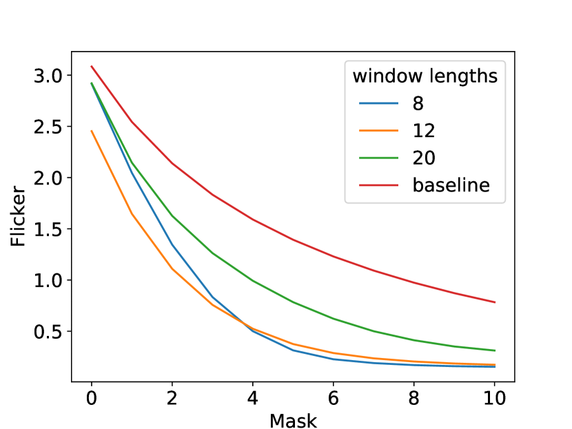
(a) English-German

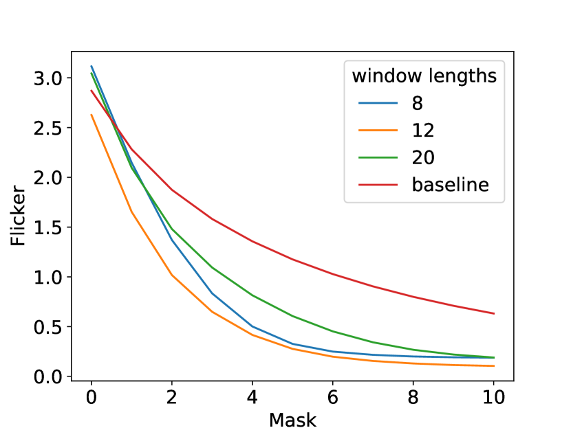
(b) English-Czech

Figure 2: Mask vs Flicker plots for different window lengths at threshold $r$ = 0.4, and the baseline.

For online SLT, since our system uses retranslation, we evaluate quality using BLEU, and flicker using normalised erasure (NE; Arivazhagan et al. 2020a). We first note that flicker is affected by both window length and thresholds – shorter windows force commitment earlier which gives lower flicker. Low thresholds promote spurious matches, make translation flicker more, whilst high thresholds force too many retranslations, and will cause extra flicker when the maximum backoff is exceeded. After exploration (Appendix C), we set the threshold to 0.4 for the rest of our experiments.

Figure 2 shows the flicker-latency tradeoff of our sliding-window approach to online SLT, as we vary the fixed mask. We can see that the tradeoff is improved at all window sizes. This improvement is because the window approach only allows updates that are within the window length. The quality of the online SLT (as measured on full sentences) is the same as the offline SLT. The flexible mask allows further improvements in flicker, for matched latency

5 Conclusion

We proposed window-based approach which works at window (of fixed length of tokens) level, and removes the need of automatic sentence-segmentation of ASR output in cascaded SLT. We experimented with English-German and English-Czech language pairs and found that our proposed approach performs better than the segmentation based translation obtaining an improvement of 1.3-2 BLEU points. We also observed that masking the output reduced the flicker by a considerable margin as compared to the baseline.

Appendix A Training data statistics

In Table 2 we show the breakdown of our training data.

Corpus	Sentence pairs
English-German
Europarl	1.79 M
Rapid	1.45 M
News Commentary	0.35 M
OpenSubtitle	22.51 M
TED corpus	206 K
MuST-C.v2	248 K
English-Czech
Europarl	645 K
ParaCrawl	14 M
CommonCrawl	161 K
News Commentary	260 K
CzEng2.0	36 M
Wikititles	410 K
Rapid	452 K

Table 2: Corpora used in training the systems

Appendix B Creation of Windowed Parallel Corpus

First, we word-align the pre-processed parallel corpus $D$ to obtain alignment $A$ using fast_align (Dyer et al., 2013). Then we concatenate all the source-target sentence pairs $(s_{k},t_{k})$ into a single, very long, pair $(s,t)$ and subsequently, revise the alignment using the Algorithm 2, so that the indexes are still correct in the concatenated corpus.

Algorithm 2 Pseudo code for collapsing a word-aligned parallel corpus into a single pair of sentences preserving the word alignments.

0:  Parallel corpus $D=\{(s_{1},t_{1}),$ $(s_{2},t_{2}),$ $\dots,$ $(s_{n},t_{n})\}$, alignment $A=\{a_{1},a_{2},...,a_{n}\},s=\epsilon,t=\epsilon$, revised alignment $A^{{}^{\prime}}=\{\}$

1:  for $k\leftarrow 1$ to $|D|$ do

2:     for each $i,j\in a_{k}$ do

3:        $i\leftarrow i+|s|$

4:        $j\leftarrow j+|t|$

5:        $A^{{}^{\prime}}\leftarrow A^{{}^{\prime}}\cup(i,j)$

6:     end for

7:     $s\leftarrow s+s_{k}$ {concatenation}

8:     $t\leftarrow t+t_{k}$ {concatenation}

9:  end for

10:  return  $s,\quad t,\quad A^{{}^{\prime}}$

Once we have combined the parallel corpus into a pair of sentences $(s,t)$, we use the revised alignment $A^{{}^{\prime}}$ to generate parallel windows of length 15-25 tokens using Algorithm 3.

Algorithm 3 Pseudo-code for extracting windows from the concatenated corpus

0:  Unsegmented source $s$, target $t$, and word alignment $A^{{}^{\prime}}$

1:  Initialize: $idx\leftarrow 0$

2:  while $idx<|t|$ do

3:     $l\leftarrow random(10,25)$

4:     $W_{t}\leftarrow t[idx:idx+l]$ {target window}

5:     $p=\min_{i}\{(i,j)\in A^{{}^{\prime}},idx\leq j<idx+l\}$

6:     $q=\max_{i}\{(i,j)\in A^{{}^{\prime}},idx\leq j<idx+l\}$

7:     $W_{s}\leftarrow s[p:q]$ {source window}

8:     $idx\leftarrow idx+l$

9:  end while

Appendix C Exploration of Match Threshold

We have two hyperparameters to consider: window length and threshold, when generating the output. We explore their combination to find the best threshold value. Table 3 shows BLEU scores with different window length and threshold. We plot the flicker against the threshold for each window in Figure 3 and we found 0.4 to be the best choice for threshold. Shorter windows force commitment earlier producing lower flicker. Low thresholds promote spurious matches making translation flicker more, whilst high thresholds force too many retranslations. We have shown the number of retranslation in Table 4 for different combination of window length and threshold. The reason why higher threshold forces too many retranslations is that even if we set higher threshold, it matches only with the match ratio between 0.5 to 0.6 on average. We have shown the average match ratio after joining every combination of window length and threshold in Table 5. We observe in Figure 3 that higher threshold increases the flicker. The reason is that: as mentioned before, in one hand, it never reaches a match of $>$ 0.6 on average thus it retranslates more and generates longer output window, on the other hand, flicker depends on actual number of token mismatch - longer window will have more mismatch for the same threshold. In addition to that, these extra retranslations incurs an increase in computation requirement. However, this increase in complexity can be easily ignored, as in real life settings, largest source of latency is waiting for new source content from the speaker (Arivazhagan et al., 2020b).

	Match Threshold ($r$)
Window($w_{l}$)	0.1	0.2	0.4	0.5	0.6	0.8
en$\rightarrow$de
8	10.8	11.3	12.3	12.5	12.4	12.5
10	12.0	12.3	12.7	12.8	12.8	12.7
12	12.5	12.7	12.9	13.0	13.0	12.9
14	12.7	12.8	13.0	13.0	12.9	12.8
16	12.9	12.9	13.1	13.1	13.1	13.0
18	13.0	13.0	13.2	13.2	13.2	13.1
20	13.1	13.0	13.2	13.2	13.2	13.2
en$\rightarrow$cs
8	8.3	9.1	9.8	10.0	10.0	9.9
10	9.5	9.7	10.2	10.3	10.2	10.2
12	10.0	10.2	10.4	10.4	10.4	10.4
14	10.2	10.4	10.5	10.4	10.5	10.4
16	10.5	10.6	10.6	10.6	10.6	10.5
18	10.5	10.5	10.6	10.6	10.6	10.5
20	10.5	10.6	10.7	10.7	10.5	10.5

Table 3: Results with different window length and threshold. Sacrebleu computed after sentence aligning each document using mwerSegmenter. Bleu scores in green have the lowest flickers.

	Match Threshold ($r$)
$w_{l}$	0.1	0.2	0.4	0.5	0.6	0.8	#windows
en$\rightarrow$de
8	1724	10513	66471	103034	140889	200441	45879
10	1303	7352	50345	82775	118991	185398	45497
12	956	6394	46528	74698	110669	178805	45115
14	702	4809	42886	69847	105207	173017	44733
16	432	4098	40447	66391	100591	167585	44351
18	308	3809	38774	65132	99410	163935	43969
20	215	3407	37358	64266	96701	162025	43587
en$\rightarrow$cs
8	2388	14757	74465	111900	148605	206238	45879
10	1257	8906	53651	84838	120135	188964	45497
12	1374	7170	44905	71432	105294	176580	45115
14	1094	5825	40480	64564	97436	169418	44733
16	806	4762	37067	60457	92346	163384	44351
18	489	4118	34710	58321	89392	158114	43969
20	292	3807	33440	57187	87418	154827	43587

Table 4: Number of extra retranslations due to history extension. $w_{l}$ is window length.

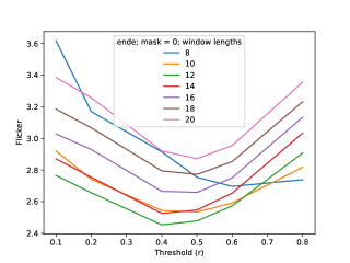
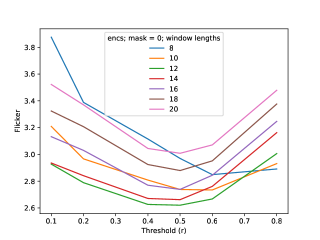
Figure 3: Threshold ($r$) vs Flicker plots.

	Match Threshold ($r$)
$w_{l}$	0.1	0.2	0.4	0.5	0.6	0.8	#windows
en$\rightarrow$de
8	0.40	0.42	0.52	0.56	0.57	0.55	45879
10	0.47	0.49	0.57	0.59	0.60	0.58	45497
12	0.51	0.52	0.59	0.62	0.62	0.59	45115
14	0.52	0.54	0.60	0.63	0.64	0.60	44733
16	0.53	0.55	0.61	0.64	0.65	0.62	44351
18	0.54	0.55	0.61	0.64	0.65	0.62	43969
20	0.55	0.56	0.62	0.64	0.65	0.62	43587
en$\rightarrow$cs
8	0.37	0.41	0.51	0.54	0.56	0.54	45879
10	0.45	0.47	0.56	0.59	0.60	0.57	45497
12	0.50	0.52	0.59	0.61	0.63	0.60	45115
14	0.53	0.54	0.61	0.63	0.65	0.61	44733
16	0.54	0.55	0.62	0.64	0.65	0.63	44351
18	0.55	0.56	0.62	0.65	0.66	0.63	43969
20	0.56	0.57	0.63	0.65	0.66	0.64	43587

Table 5: Average match ratio after joining all the windows across different window length and threshold. We define average match ratio as $\frac{1}{\#window}\sum^{\#window}\frac{\mathrm{match\_length}}{\mathrm{output\_window\_length}}$

References

- Akhbardeh et al. (2021) Farhad Akhbardeh, Arkady Arkhangorodsky, Magdalena Biesialska, Ondřej Bojar, Rajen Chatterjee, Vishrav Chaudhary, Marta R. Costa-jussa, Cristina España-Bonet, Angela Fan, Christian Federmann, Markus Freitag, Yvette Graham, Roman Grundkiewicz, Barry Haddow, Leonie Harter, Kenneth Heafield, Christopher Homan, Matthias Huck, Kwabena Amponsah-Kaakyire, Jungo Kasai, Daniel Khashabi, Kevin Knight, Tom Kocmi, Philipp Koehn, Nicholas Lourie, Christof Monz, Makoto Morishita, Masaaki Nagata, Ajay Nagesh, Toshiaki Nakazawa, Matteo Negri, Santanu Pal, Allahsera Auguste Tapo, Marco Turchi, Valentin Vydrin, and Marcos Zampieri. 2021. Findings of the 2021 conference on machine translation (WMT21). In Proceedings of the Sixth Conference on Machine Translation, pages 1–88, Online. Association for Computational Linguistics.
- Arivazhagan et al. (2020a) Naveen Arivazhagan, Colin Cherry, Te I, Wolfgang Macherey, Pallavi Baljekar, and George Foster. 2020a. Re-Translation Strategies For Long Form, Simultaneous, Spoken Language Translation. In ICASSP 2020 - 2020 IEEE International Conference on Acoustics, Speech and Signal Processing (ICASSP).
- Arivazhagan et al. (2020b) Naveen Arivazhagan, Colin Cherry, Wolfgang Macherey, and George Foster. 2020b. Re-translation versus streaming for simultaneous translation. In Proceedings of the 17th International Conference on Spoken Language Translation, pages 220–227, Online. Association for Computational Linguistics.
- Barrault et al. (2020) Loïc Barrault, Magdalena Biesialska, Ondřej Bojar, Marta R. Costa-jussà, Christian Federmann, Yvette Graham, Roman Grundkiewicz, Barry Haddow, Matthias Huck, Eric Joanis, Tom Kocmi, Philipp Koehn, Chi-kiu Lo, Nikola Ljubešić, Christof Monz, Makoto Morishita, Masaaki Nagata, Toshiaki Nakazawa, Santanu Pal, Matt Post, and Marcos Zampieri. 2020. Findings of the 2020 conference on machine translation (WMT20). In Proceedings of the Fifth Conference on Machine Translation, pages 1–55, Online. Association for Computational Linguistics.
- Cho et al. (2017) Eunah Cho, Jan Niehues, and Alex Waibel. 2017. NMT-Based Segmentation and Punctuation Insertion for Real-Time Spoken Language Translation. Proceedings of Interspeech, pages 2645–2649.
- Dyer et al. (2013) Chris Dyer, Victor Chahuneau, and Noah A. Smith. 2013. A simple, fast, and effective reparameterization of IBM model 2. In Proceedings of the 2013 Conference of the North American Chapter of the Association for Computational Linguistics: Human Language Technologies, pages 644–648, Atlanta, Georgia. Association for Computational Linguistics.
- Junczys-Dowmunt et al. (2018) Marcin Junczys-Dowmunt, Roman Grundkiewicz, Tomasz Dwojak, Hieu Hoang, Kenneth Heafield, Tom Neckermann, Frank Seide, Ulrich Germann, Alham Fikri Aji, Nikolay Bogoychev, André F. T. Martins, and Alexandra Birch. 2018. Marian: Fast neural machine translation in C++. In Proceedings of ACL 2018, System Demonstrations, pages 116–121, Melbourne, Australia. Association for Computational Linguistics.
- Khayrallah and Koehn (2018) Huda Khayrallah and Philipp Koehn. 2018. On the impact of various types of noise on neural machine translation. In Proceedings of the 2nd Workshop on Neural Machine Translation and Generation, pages 74–83, Melbourne, Australia. Association for Computational Linguistics.
- Kudo and Richardson (2018) Taku Kudo and John Richardson. 2018. SentencePiece: A simple and language independent subword tokenizer and detokenizer for neural text processing. In Proceedings of the 2018 Conference on Empirical Methods in Natural Language Processing: System Demonstrations, pages 66–71, Brussels, Belgium. Association for Computational Linguistics.
- Li et al. (2021) Daniel Li, I Te, Naveen Arivazhagan, Colin Cherry, and Dirk Padfield. 2021. Sentence boundary augmentation for neural machine translation robustness. In ICASSP 2021-2021 IEEE International Conference on Acoustics, Speech and Signal Processing (ICASSP), pages 7553–7557. IEEE.
- Ma et al. (2019) Mingbo Ma, Liang Huang, Hao Xiong, Renjie Zheng, Kaibo Liu, Baigong Zheng, Chuanqiang Zhang, Zhongjun He, Hairong Liu, Xing Li, Hua Wu, and Haifeng Wang. 2019. STACL: Simultaneous translation with implicit anticipation and controllable latency using prefix-to-prefix framework. In Proceedings of the 57th Annual Meeting of the Association for Computational Linguistics, pages 3025–3036, Florence, Italy. Association for Computational Linguistics.
- Macháček et al. (2021) Dominik Macháček, Matúš Žilinec, and Ondřej Bojar. 2021. Lost in interpreting: Speech translation from source or interpreter? In Proceedings of INTERSPEECH 2021, pages 2376–2380, Baxas, France. ISCA.
- Matusov et al. (2005) Evgeny Matusov, Gregor Leusch, Oliver Bender, and Hermann Ney. 2005. Evaluating machine translation output with automatic sentence segmentation. In Proceedings of the Second International Workshop on Spoken Language Translation, Pittsburgh, Pennsylvania, USA.
- Niehues et al. (2016) Jan Niehues, Thai Son Nguyen, Eunah Cho, Thanh-Le Ha, Kevin Kilgour, Markus Muüller, Matthias Sperber, Sebastian Stüker, and Alex Waibel. 2016. Dynamic transcription for low-latency speech translation. In Proceedings of Interspeech.
- Papineni et al. (2002) Kishore Papineni, Salim Roukos, Todd Ward, and Wei-Jing Zhu. 2002. Bleu: a method for automatic evaluation of machine translation. In Proceedings of the 40th Annual Meeting of the Association for Computational Linguistics, pages 311–318, Philadelphia, Pennsylvania, USA. Association for Computational Linguistics.
- Post (2018) Matt Post. 2018. A call for clarity in reporting BLEU scores. In Proceedings of the Third Conference on Machine Translation: Research Papers, pages 186–191, Brussels, Belgium. Association for Computational Linguistics.
- Sennrich et al. (2016) Rico Sennrich, Barry Haddow, and Alexandra Birch. 2016. Neural machine translation of rare words with subword units. In Proceedings of the 54th Annual Meeting of the Association for Computational Linguistics (Volume 1: Long Papers), pages 1715–1725, Berlin, Germany. Association for Computational Linguistics.
- Vaswani et al. (2017) Ashish Vaswani, Noam Shazeer, Niki Parmar, Jakob Uszkoreit, Llion Jones, Aidan N. Gomez, Lukasz Kaiser, and Illia Polosukhin. 2017. Attention Is All You Need. CoRR, abs/1706.03762.