Pair correlation function based on Voronoi topology

Abstract

The pair correlation function (PCF) has proven an effective tool for analyzing many physical systems due to its simplicity and its applicability to simulated and experimental data. However, as an averaged quantity, the PCF can fail to capture subtle structural differences in particle arrangements, even when those differences can have a major impact on system properties. Here, we use Voronoi topology to introduce a discrete version of the PCF that highlights local inter-particle topological configurations. The advantages of the Voronoi PCF are demonstrated in several examples including crystalline, hyperuniform, and active systems showing clustering and giant number fluctuations.

I Introduction

Many physical, chemical, and biological systems are studied as large sets of point-like particles whose arrangement in space determines many system properties. Crystals have a relatively simple and elegant structure in which particle positions can be described with finite data (i.e., a periodically repeating unit cell). However, in general, particles may be arranged in more complex ways that cannot be described in such a simple manner torquato2002random . The distribution of molecules in fluids terban2021structural , celestial bodies in galaxies babu1996spatial , trees in forests Velazquez2016 , and animals moving in groups vicsek1995novel are but several examples. The appearance of discrete point patterns in multiple disciplines and on various length scales highlights the need for general methods for describing their structure, in both quantitative and qualitative terms diggle1976statistical ; Ripley2005 ; Spodarev2013 ; morse2014geometric ; morse2016geometric ; patania2017topological ; carlsson2020topological ; skinner2021topological ; skinner2023topological .

The pair correlation function (pcf) was introduced in the early twentieth century as a method of describing structure in spatial point patterns. In particular, the pcf details the distribution of distances between particles within a system, and can therefore be used to infer, among other features, system length scales. Another reason for the tremendous success of the pcf is its close relationship with X-ray diffraction through the structure factor. These tools have facilitated an accurate view of the atomic-level structure of countless materials billinge2019rise .

The pcf, however, is limited in several respects. Most importantly, it is sensitive to small random perturbations, such as those caused by temperature or measurement errors, which do not typically affect structural classification kittel1976introduction . Post-processing is subsequently necessary to distinguish artifacts associated with noise from indicators of structurally significant features. At the same time, it is rather insensitive to changes in a small fraction of particles such as defects or local symmetries, that may be averaged out globally, even though such details can have a significant effect on macroscopic properties torquato2002random . For these reasons, despite its great success in providing deep understanding of crystalline and other ordered systems, its utility in studying disordered ones has been comparatively limited kardarfields ; billinge2019rise .

In this paper we introduce a discrete version of the pcf built on Voronoi topology lazar2015topological ; leipold2016statistical , and which we thus name the Voronoi pair correlation function (vpcf). It is complementary to the classical pcf in several respects: i. It is naturally invariant under rescaling of length, as well as translations and rotations. ii. It is inherently robust to random perturbations and measurement errors . iii. It is sensitive to local order and symmetries. As demonstrated below, the vpcf proves useful in studying both ordered and disordered systems.

Recall the definition of the two-point correlation function, as the two- dimensional marginal distribution, $p^{(2)}$, normalized by the average particle density $\rho$ kardarfields . In many systems, $p^{(2)}$ only depends on distances between particles. One then defines the radial distribution function as

$$g(r)=\frac{1}{\rho a(r)}p^{(2)}(|{\bf r}_{1}-{\bf r}_{2}|=r),$$ (1)

where $a(r)$ is the perimeter or surface area of the $d$-dimensional spherical shell; $a(r)=2\pi r$ in two dimensions and $a(r)=4\pi r^{2}$ in three dimensions. Intuitively, if the probabilities of finding two particles at locations a distance $r_{0}$ apart are independent, then $g(r_{0})=1$. For this reason, in systems with a finite correlation length, $g(r\to\infty)=1$. In particular, for an ideal gas with any density, $g(r)\equiv 1$. In ideal periodic systems, the set of interparticle distances is necessarily discrete. In more general systems, such as those described by thermodynamic ensembles, this set is typically continuous. Thus, $g(r)$ can distinguish between different ordered spatial configurations as well as some disordered ones Torquato2018 ; kardarfields .

\begin{overpic}[trim=52.63759pt 49.081pt 52.63759pt 49.081pt,clip,height=86.07425pt]{Fig1a}\put(-2.0,90.0){ {\fcolorbox{black}{white}{(a)}}} \end{overpic} \begin{overpic}[trim=52.63759pt 49.081pt 52.63759pt 49.081pt,clip,height=86.07425pt]{Fig1b}\put(-2.0,90.0){ {\fcolorbox{black}{white}{(b)}}} \end{overpic} \begin{overpic}[trim=52.63759pt 49.081pt 52.63759pt 49.081pt,clip,height=86.07425pt]{Fig1c}\put(-2.0,90.0){ {\fcolorbox{black}{white}{(c)}}} \end{overpic} \begin{overpic}[trim=52.63759pt 49.081pt 52.63759pt 49.081pt,clip,height=86.07425pt]{Fig1d}\put(-2.0,90.0){ {\fcolorbox{black}{white}{(d)}}} \end{overpic} \begin{overpic}[trim=52.63759pt 49.081pt 52.63759pt 49.081pt,clip,height=86.07425pt]{Fig1e} \put(-2.0,90.0){ {\fcolorbox{black}{white}{(e)}}}\end{overpic}

Figure 1: A central particle and its Voronoi neighbors, colored by Voronoi distances from the central particle: (a) a low temperature, defect-free hexagonal crystal constructed using molecular dynamics and a Lennard-Jones potential, (b) a random organization example of a disordered hyperuniform system, (c) an ideal gas, (d) a Vicsek model of collective motion, and (e) a clustered Poisson process. A modified version of VoroTop vorotop has been used to illustrate the systems.

\begin{overpic}[trim=28.45274pt 25.60747pt 25.60747pt 25.60747pt,clip,height=84.55576pt]{Fig2a}\put(-2.0,90.0){ {\fcolorbox{black}{white}{(a)}}} \end{overpic} \begin{overpic}[trim=28.45274pt 25.60747pt 25.60747pt 25.60747pt,clip,height=84.55576pt]{Fig2b}\put(-2.0,90.0){ {\fcolorbox{black}{white}{(b)}}} \end{overpic} \begin{overpic}[trim=28.45274pt 25.60747pt 25.60747pt 25.60747pt,clip,height=84.55576pt]{Fig2c}\put(-2.0,90.0){ {\fcolorbox{black}{white}{(c)}}} \end{overpic} \begin{overpic}[trim=28.45274pt 25.60747pt 25.60747pt 25.60747pt,clip,height=84.55576pt]{Fig2d}\put(-2.0,90.0){ {\fcolorbox{black}{white}{(d)}}} \end{overpic} \begin{overpic}[trim=28.45274pt 25.60747pt 25.60747pt 25.60747pt,clip,height=84.55576pt]{Fig2e} \put(-2.0,90.0){ {\fcolorbox{black}{white}{(e)}}}\end{overpic}

Figure 2: A central particle and $k$-shells of its Voronoi neighbors, colored by Voronoi distances from the central particle: (a) a low temperature, defect-free hexagonal crystal constructed using molecular dynamics and a Lennard-Jones potential, (b) a random organization example of a disordered hyperuniform system, (c) an ideal gas, (d) a Vicsek model of collective motion, and (e) a clustered Poisson process. Quantitative information about these shells captures information about structural order.

II A topological
pair correlation function

To define a topological version of the pcf, we first consider the Voronoi tessellation, a subdivision of a system into regions, called Voronoi cells, that are closer to one particle than to any other voronoi1908nouvelles ; lazar2022voronoi . Formally, given a discrete set of points (particle positions) $\{s_{1},s_{2},\ldots\}\subset\mathbb{R}^{d}$, the Voronoi cell of particle $i$ is the set

$$V(s_{i})=\{x\in\mathbb{R}^{d}\,|\,d(x,s_{i})\leq d(x,s_{j})\},$$ (2)

where $d(x,y)$ is the standard Euclidean metric. In two dimensions, Voronoi cells are convex polygons, while in three dimensions they are convex polyhedra.

Voronoi tessellations induce a discrete metric on particle systems. We define distances between particles in terms of shortest paths, where path lengths are quantified by the number of Voronoi cells that need be traversed in moving from one particle to another. Figure 1 illustrates several two-dimensional systems and their Voronoi tessellations; particles are colored according to their Voronoi distances from a central reference particle. Figure 2 depicts zoom-outs of the same systems, but showing only several shells – sets of particles located at a fixed Voronoi distance from a central reference particle.

To quantify the patterns observed in the figures above, we next count the number of neighbors at each fixed Voronoi distance from a reference particle, and average over all particles. In a defect-free hexagonal crystal, for example, each particle has exactly $6k$ neighbors at a Voronoi distance $k$; see Fig. 1(a). This is the case even when particles are displaced by small perturbations, such as those resulting from thermal vibrations. In more general systems, however, there can be variation in the number of neighbors at different Voronoi distances; see Figs. 1(b-e). We use $k$-neighbors to refer to neighbors located at a Voronoi distance $k$ away from a reference particle, and $p_{i}(k)$ to denote the number of $k$-neighbors of particle $i$. We use $u(k)$ to denote the average number of $k$-neighbors of particles in a system containing $N$ particles:

$$u(k)=\left<\frac{1}{N}\sum_{i}^{N}p_{i}(k)\right>,$$ (3)

where $\left<\cdot\right>$ denotes ensemble averaging and may also include variation in $N$.

One of the nice properties of the classical pcf is its normalization, which provides an intuitive physical meaning. In contrast to the classical pcf, however, which requires rescaling of lengths, the vpcf is determined by combinatorial features of Voronoi tessellations, which are naturally invariant under rescaling, and therefore no renormalization of length is necessary. We still, however, need to normalize $u(k)$, which diverges as $k\to\infty$, complicating the comparison of systems. Accordingly, and in analogy to the classical pcf, we normalize $u(k)$ using data for an ideal gas, denoted $u_{\rm id}(k)$. We thus define the Voronoi pair correlation function $v(k)$ for a general particle system $S$ as

$$v_{S}(k)=\frac{u_{S}(k)}{u_{\rm id}(k)}.$$ (4)

In all systems considered here, $u(k)$ grows asymptotically linearly with $k$. This is expected under some reasonable assumptions for spatial systems such as a finite variance in the number of neighbors. The ratio between the asymptotic linear growth rate of $u_{S}(k)$ and that of $u_{\rm id}(k)$ provides the asymptotic value of $v_{S}(k)$ as $k\to\infty$. Determining the vpcf only requires tools for the computation of Voronoi cells, or its dual Delaunay triangulation aurenhammer2013voronoi , and shortest paths in networks. These tools are readily available in many software packages, making the vpcf simple to compute. Alternatively, VoroTop vorotop offers an efficient and parallelizable package of Voronoi topology computational tools, including the vpcf.

III Examples

We now demonstrate the utility of the vpcf by considering several two-dimensional systems illustrated in Figs. 1 and 2: a low-temperature, defect-free hexagonal crystal, a random organization example of a disordered hyperuniform system, an ideal gas, a snapshot of a Vicsek simulation , and a Poisson cluster process; Fig. 3 plots $v(k)$ for each.

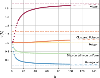
Figure 3: The Voronoi pair correlation function $v(k)$ for the systems depicted in Fig. 1 with roughly 100,000 particles each. Shown are the data (solid points), a least-squares fit to Eq. 5 (dotted line), and the asymptotic values $v(\infty)$ (dashed line).

III.1 Poisson point process

A Poisson point process is a mathematical model of an ideal gas, in which points are independently and uniformly distributed in a fixed region lazar2013statistical ; see Fig. 1(c). Although the full distribution of first nearest neighbors is known analytically calka2003explicit , even the average number of $k$-neighbors for general $k$ is not.

As mentioned earlier, we expect the average number of $k$-neighbors to grow asymptotically linearly with $k$, analogous to the linear growth of the perimeter of a circle with its radius. Simulation data suggest that the average number of $k$-neighbors in equilibrium two-dimensional systems is approximated by a function of the form

$$u(k)=c_{0}+c_{1}k+c_{2}k^{\frac{1}{2}}+c_{3}k^{\frac{1}{4}},$$ (5)

ignoring lower-order terms, and with constants $c_{i}$ that are system specific. For the ideal gas, a least-squares fit of $u(k)$ constrained by $u(1)=6$ yields $c_{0}=18.77$, $c_{1}=12.58$, $c_{2}=-0.49$, and $c_{3}=-24.9$; additional details can be found in the appendix. The constant $c_{1}=12.58$ is noteworthy, since it is the linear growth rate of $k$-neighbors in the ideal gas, and will determine the asymptotic behavior of $v(k)$ for general systems.

III.2 Hexagonal lattice

The hexagonal crystal, illustrated in Fig. 1(a), is among the simplest and most studied two-dimensional physical systems. As mentioned above, the number of $k$-neighbors of each particle is exactly $6k$, and so $u(k)=6k$. Dividing this by the linear term obtained for the ideal gas, $c_{1}=12.58$, we have $v(k\to\infty)=0.477$. Figure 3 shows that $v(k)$ for the hexagonal crystal is smallest among all systems considered.

III.3 Poisson cluster process

A hallmark of active systems is giant number fluctuations ramaswamy2017active . In these systems, activity drives clustering peruani2006nonequilibrium , phase separation cates2015motility , or arrested phase separation worlitzer2021motility . Activity and out-of-equilibrium statistics are thus manifested in spatial configurations. The effectiveness of the vpcf in detecting such patterns is illustrated by consideration of a Matérn cluster point process, an example toy model of disordered systems that exhibits clustering Spodarev2013 . In this model, a set of “parent” points is generated through a homogeneous Poisson point process with intensity, or average density of points per unit area, $\phi$. Next, around each parent point is placed a disk of radius $r$ in which “children” points are generated through independent homogeneous Poisson point processes with intensity $\lambda$. The result is a point process with intensity $\pi r^{2}\phi\lambda$, and in which points are grouped into clusters, possibly overlapping, with an average number of points $\pi r^{2}\lambda$ in each. Figure 1(d) shows an example system with $\phi=1$, $r=0.2$, and $\lambda=500$, and Fig. 3 shows its vpcf. In this case we find that $v(k\to\infty)=1.26$.

To highlight the sensitivity of the vpcf to subtle differences in structure, we next consider a modified version of the Matérn cluster point process that includes “defects”. Specifically, while the majority of children points are located in clusters as described above, a fraction of them, $0<p<1$, are instead distributed randomly in the region. These defect particles can be thought of as being generated by a Poisson point process with intensity $p\pi r^{2}\phi\lambda$; see Fig. 4(a) for an example when $p=0.01$.

\begin{overpic}[width=216.81pt]{Fig4} \put(0.0,44.5){ {\fcolorbox{black}{white}{\footnotesize(a)}}} \put(91.0,44.5){ {\fcolorbox{black}{white}{\footnotesize(b)}}} \end{overpic}

Figure 4: (a) Poisson cluster process with $\phi=10$, $r=0.05$, and $\lambda=100$, and in which a fraction $p=0.01$ of children points are labeled as defects (red) and randomly distributed in space instead of in disks centered at parent points. (b) The Voronoi pair correlation function $v(k)$ for the original Matérn point process and the version with defects. Inset: the classical pair correlation functions of the two systems are indistinguishable.

When $p$ is small, the vast majority of particles belong to densely populated disk-shaped clusters, and the presence of these isolated defects cannot be detected by the classical pcf. In contrast, these defects significantly alter the Voronoi tessellation and the resulting vpcf. Figure 4(b) illustrates the noticeable difference between the vpcf of the original system and that with defects, demonstrating that the vpcf can detect structural features that are “hidden” to the pcf. This might be of interest in analyzing networks in which hubs in otherwise unpopulated areas might significantly impact network structure by reducing path distances between points through local rewiring.

III.4 Disordered hyperuniformity

Hyperuniform structures are point patterns in which long-range spatial fluctuations are suppressed, as compared to an ideal gas Hexner2015 ; Hexner2017 ; Torquato2018 . More formally, a system is said to be hyperuniform if its structure factor $S(q)$ vanishes for $q\to 0$. Recently, it has been shown that hyperuniformity can be detected by considering the entropy of the many-body distribution of positions Ariel2020 .

Examples of hyperuniform systems include crystals and quasicrystals. More intriguingly, disordered systems can exhibit hyperuniformity too.

\begin{overpic}[width=216.81pt]{Fig5} \put(7.2,43.5){ {\fcolorbox{black}{white}{\footnotesize(a)}}} \put(51.7,43.5){ {\fcolorbox{black}{white}{\footnotesize(b)}}} \end{overpic}

Figure 5: (a) The Voronoi pair correlation function $v(k)$ for the random organization model at different densities $\rho$. (b) The simulation time (red line) to reach an absorbing state or a steady state, and the asymptotic value $v(\infty)$ while varying the densities (blue line); the scale is the same as in (a). The minimum of $v(\infty)$ at $\rho=0.35$ indicates the critical density for hyperuniformity (black dashed line).

One of the elegant models exhibiting disordered hyperuniformity is the random organization model Hexner2015 ; Hexner2017 . In this model, $N$ disks of fixed diameter $r$ are randomly and independently placed in a domain $[0,L]^{2}$ with periodic boundaries. Overlapping disks are marked as active and are then displaced; this procedure is repeated until either no disks overlap, in which case the system is said to have reached an absorbing state, or until the fraction of active disks is constant in time, in which case the system is said to have reached a steady state. The control parameter is the area fraction of disks, $\rho=N\pi r^{2}/L^{2}$. At low densities, an absorbing state is reached, while at high densities a steady state is reached. The transition occurs at a critical density $\rho_{c}$, which is smaller than the maximum packing fraction of disks in $[0,L]^{2}$. Interestingly, exactly at the transition, the system becomes hyperuniform, i.e., large scale density fluctuations are suppressed Hexner2015 ; Hexner2017 ; Torquato2018 ; Ariel2020 .

Figure 5(a) shows the vpcf for random organization models with different densities for 50,000 particles. At the critical density $\rho_{c}$, the vpcf decreases fastest with increasing $k$. Indeed, the large distance limit $v(k\to\infty)$ exhibits a cusp with a minimum exactly at the critical density; see Fig. 5(b). Intuitively, a hyperuniform system is similar to a crystal in terms of the number of Voronoi neighbors. As a result, the vpcf is closer to that of a crystal than to that of a non-hyperuniform system; see Fig. 3.

This example illustrates the strength of the vpcf as a general-purpose tool for analyzing structure in particle systems. In particular, the vpcf can detect phase transitions which are characterized by structural changes. Moreover, it is applied directly in real space rather than in Fourier space. This is important, as it is often technically difficult to identify hyperuniformity from the classical pcf or structure factor directly, as finite size effects often prevent the structure factor from vanishing at small wave numbers. In addition, sampling very short wave numbers may not be experimentally accessible ricouvier2017optimizing . However, note that $v(\infty)<1$ is not an indication of hyperuniformity.

\begin{overpic}[trim=7.11317pt 1.42262pt 7.11317pt 2.84526pt,clip,width=149.59943pt]{Fig6a.eps} \put(30.0,63.0){ {\fcolorbox{black}{white}{\footnotesize(a)}}} \end{overpic}

\begin{overpic}[trim=7.11317pt 1.42262pt 7.11317pt 2.84526pt,clip,width=149.59943pt]{Fig6b.eps} \put(30.0,63.0){ {\fcolorbox{black}{white}{\footnotesize(b)}}} \end{overpic}

\begin{overpic}[trim=7.11317pt 1.42262pt 7.11317pt 2.84526pt,clip,width=149.59943pt]{Fig6c.eps} \put(30.0,63.0){ {\fcolorbox{black}{white}{\footnotesize(c)}}} \end{overpic}

Figure 6: The vpcf for the (a) standard and (b) diffusion-modified RSA systems. A phase transition can be observed in the diffusion-modified system near $\rho=0.51$. (c) This phase transition can be observed more clearly by considering the first finite difference of the vpcf.

III.5 Random sequential adsorption

While this short paper cannot address the full breadth of hyperuniform systems torquato2021local , we briefly consider a second example: random sequential adsorption (RSA) and a diffusion-modified version of it; these are widely-studied models of adsorption and surface attachment lavalle1999extended ; torquato2006random .

The standard RSA model in two dimensions is defined as follows. Consider a domain $[0,L]^{2}$ with periodic boundary conditions. Particles are placed sequentially into the domain. After placing $n$ particles, the position of particle $n+1$ is drawn uniformly within the domain. If the new position overlaps with any of the previous $n$ particles, it is discarded and redrawn. The process stops when no available positions remain. It has been shown numerically that the average maximal surface area is about 0.547 lavalle1999extended ; torquato2006random .

We also implemented a variation of the model with surface diffusion lavalle1999extended . Every time a position is discarded, the particles with which the candidate position overlapped are displaced randomly. Displacements in each coordinate are taken as independent Gaussians with zero mean and standard deviation of 0.01.

Figures 6(a) and (b) illustrate $v(k)$ for several $k$ over a range of densities in the standard and diffusion-modified systems. Although the data are similar, the diffusion-modified system illustrates a (continuous) phase transition close to the critical density $\rho=0.51$. Figure 6(c) shows a finite difference estimate of the derivative of $v(k)$ with respect to $\rho$. While $v(k)$ decreases with increasing density $\rho$, its second derivative changes sign at this critical point.

III.6 Three dimensional examples

Ideas developed in this paper immediately generalize to higher dimensions. We briefly illustrate the application of the vpcf to three-dimensional systems. VoroTop [23] was used to compute the average number of $k$-neighbors in a three-dimensional ideal gas and we then used those data to normalize the vpcf of other particle systems described below and summarized in Fig. 7.

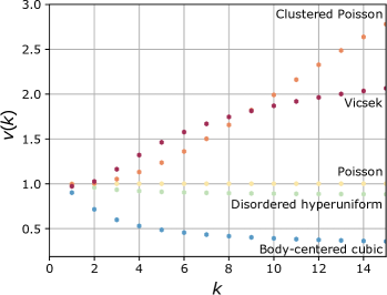
Figure 7: The Voronoi pair correlation function for three-dimensional systems, each with roughly 500,000 particles.

The ideal gas. We constructed 50 independent copies, each with one million particles, and calculated the vpcf in each of them. In two dimensions the number of $k$-neighbors grows linearly in $k$, as the perimeter of a circle is proportional to its radius. The proportion constant quantifies the discrete nature of the conversion from a continuous perimeter to a discretized $k$-shell, and also the degree to which the $k$-shells are circular. In three dimensions, the surface area of a sphere grows as the square of its radius, and so we expect that the number of $k$-neighbors, a discrete analog of surface area, will grow approximately linearly in $k^{2}$. We thus considered functions of the form:

$$u(k)=c_{0}+c_{1}k+c_{2}k^{2}$$ (6)

to describe the number of $k$-neighbors in a three-dimensional ideal gas. A least squares fit of the simulation data results in constants $c_{0}=381$, $c_{1}=-166$, and $c_{2}=42.7$. We note that while this form accurately fits data for large $k$, it is less accurate for small $k$. For this reason we use actual numerical data to normalize $v(k)$ for other systems.

Perturbed crystals. The three-dimensional body-centered cubic crystal can be considered an analog of the two-dimensional hexagonal crystal in the sense that its Voronoi cells are topologically stable – small perturbations of particle positions do not result in topological changes in the Voronoi cells. In this system, each Voronoi cell is a truncated octahedron with eight hexagonal faces and six square ones. Figure 7 shows that $v(k)$ is smallest for the body-centered cubic crystal among all three-dimensional systems considered.

Poisson cluster process. We constructed Poisson cluster processes in the same manner as in two dimensions. In particular, we studied a system with $\phi=10$, $r=0.05$, and $\lambda=100$. The apparent unbounded growth of $v(k)$ for this system might be attributed to the system sizes considered. With the increase in dimension, the number of $k$-neighbors grow, and hence significantly larger systems must be considered to obtain accurate estimates of $v(k)$ for large $k$. Meanwhile, the computational expense to compute them also increases.

Vicsek model. We also looked at a quasi-three dimensional system derived from a Vicsek model. We ran a classical Vicsek model vicsek1995novel with $10^{6}$ particles, unit density, and uniform noise in $[-0.6\pi,0.6\pi]$; simulations were run for $10^{5}$ time steps. At the end of the simulations, we rescaled the particle directions, which normally are measured in angles in $[0,2\pi]$ with periodic boundary conditions to lie in $[0,1]$ instead. Thus, we obtain a quasi-three dimensional representation of the data.

Disordered hyperuniform. We constructed three-dimensional analogs of the two-dimensional random organization model described above. Figure 8 illustrates the same critical behavior in three dimensions observed in two dimensions. In particular, when $\rho$ is below a critical threshold, in this case roughly $0.1$, the vpcf decreases with increasing density $\rho$, after which it increases. This criticality is mirrored in the simulation time necessary to reach an absorbing or steady state.

\begin{overpic}[width=216.81pt]{Fig8} \put(40.2,44.5){ {\fcolorbox{black}{white}{\footnotesize(a)}}} \put(82.75,44.5){ {\fcolorbox{black}{white}{\footnotesize(b)}}} \end{overpic}

Figure 8: (a) The Voronoi pair correlation function $v(k)$ for the random organization model in three dimensions at different densities $\rho$. (b) The simulation time (red line) to reach an absorbing state or a steady state, and the asymptotic value $v(\infty)$ while varying the densities (blue line); the scale is the same as in (a). The minimum of $v(10)$ at $\rho=0.10$ indicates the critical density for hyperuniformity (black dashed line).

IV Discussion

Recent decades have seen the rapid development and application of topological methods in analyzing scientific data patania2017topological ; carlsson2020topological , contributing to progress in many problems in the physical and biological sciences skinner2021topological ; skinner2023topological . Much of the success of such methods results from their segmentation of data in high-dimensional configuration spaces associated with the problem, instead of in lower-dimensional images of those spaces obtained through continuous functions landweber2016fiber .

The discrete Voronoi pair correlation function provides a natural topological version of the classical pair correlation function. The vpcf succinctly captures structural information about particle systems in a manner that is naturally scale invariant, and which is also stable with respect to small perturbations, such as those associated with temperature or measurement error. At the same time it is able to detect structural features “hidden” from classical, purely geometric, methods. This might be useful, for example, in studying the glass transition, which is commonly believed to occur without or with only minimal structural changes janssen2018mode , and for which the classical pcf is ineffective.

The present paper complements recent advances in the application of Voronoi analysis to the study of ordered and disordered particle systems. Morse and Corwin considered the average number of nearest Voronoi neighbors, as well as geometric features of the Voronoi cells, to classify the jamming transition morse2014geometric . Klatt and Torquato looked at volumes, surface areas and mean widths of Voronoi cells to characterize the structure of maximally random jammed sphere packings klatt2014characterization . They further studied correlations of these geometric features among neighboring Voronoi cells to provide a more refined structural description of disordered particle systems klatt2014characterization . In contrast to these predominantly geometric approaches, Skinner and coauthors skinner2021topological ; skinner2023topological develop a topological approach towards quantifying the similarity and difference between Delaunay triangulations obtained from disordered systems. Their method was used to identify structural differences among several biological systems, highlighting the scientific diversity of applications that can benefit from topological methods.

We note that although $v(k)$ captures much structural information in a discrete sequence of numbers, important information is lost due to averaging data over all particles. We can thus also consider higher-order moments of the distribution of $k$-neighbors. Such information might distinguish distinct crystal structures that cannot be distinguished when considering $v(k)$ alone.

Finally, we have focused most of our attention on two-dimensional systems largely for simplicity of presentation and for ease of illustration. We anticipate that higher dimensions will provide interesting challenges as well as opportunities that do not arise in two dimensions. In particular, the shapes of $k$-shells are expected to have significantly richer features.

Acknowledgements. This work was supported by the Data Science Institute at Bar-Ilan University.

Figure 9: Points illustrate the average number of $k$-neighbors of all particles in 100 samples of an ideal gas in two dimensions, each containing half a million points. The fitted curve is of the form given by Eq. 5; error bars are too small to see.

Appendix A Appendix: semi-analytic form of $u_{PV}(k)$

Simulation data suggest that the average number of $k$-neighbors in equilibrium two-dimensional systems is accurately approximated by a function of the form

$$u(k)=c_{0}+c_{1}k+c_{2}k^{\frac{1}{2}}+c_{3}k^{\frac{1}{4}}.$$ (5)

In particular, the number of $k$-neighbors grows asymptotically linearly in $k$. This can be viewed as a discretized version of the linear relationship between the perimeter of a circle, discretized in $k$-shells, and its radius.

To obtain accurate estimates of the parameters $c_{i}$ for the homogeneous Poisson point process, we constructed 100 systems, each containing half a million particles uniformly distributed in a square with periodic boundaries, and computed $u(k)$ in each of them for $1\leq k\leq 100$. Averaging the data and using a weighted least squares fit to Eq. 5, constrained so that $u(1)=6$, yields $c_{0}=18.77$, $c_{1}=12.58$, $c_{2}=-0.49$, and $c_{3}=-24.9$, with the least uncertainty in $c_{1}$. This provides an excellent fit to the observed data for both large and small $k$; the root mean square deviation is $0.01$.

Figure 9 illustrates these data and a fit of $u(k)$ using the parameters $c_{i}$ as described. As can be seen from the inset figures, Eq. 5 with the fitted parameters accurately approximates the observed data for both low and high values of $k$.

References

- (1) S. Torquato, Random Heterogeneous Materials: Microstructure and Macroscopic Properties. Springer-Verlag, New York, 2002.
- (2) M. W. Terban and S. J. Billinge, “Structural analysis of molecular materials using the pair distribution function,” Chemical Reviews, vol. 122, no. 1, pp. 1208–1272, 2021.
- (3) G. J. Babu and E. D. Feigelson, “Spatial point processes in astronomy,” Journal of Statistical Planning and Inference, vol. 50, no. 3, pp. 311–326, 1996.
- (4) E. Velázquez, I. Martínez, S. Getzin, K. A. Moloney, and T. Wiegand, “An evaluation of the state of spatial point pattern analysis in ecology,” Ecography, vol. 39, no. 11, pp. 1042–1055, 2016.
- (5) T. Vicsek, A. Czirók, E. Ben-Jacob, I. Cohen, and O. Shochet, “Novel type of phase transition in a system of self-driven particles,” Physical Review Letters, vol. 75, no. 6, p. 1226, 1995.
- (6) P. J. Diggle, J. Besag, and J. T. Gleaves, “Statistical analysis of spatial point patterns by means of distance methods,” Biometrics, vol. 32, no. 3, pp. 659–667, 1976.
- (7) B. D. Ripley, Spatial Statistics. John Wiley & Sons, 2005.
- (8) E. Spodarev, Stochastic Geometry, Spatial Statistics and Random Fields: Asymptotic Methods, vol. 2068. Springer, 2013.
- (9) P. K. Morse and E. I. Corwin, “Geometric signatures of jamming in the mechanical vacuum,” Physical Review Letters, vol. 112, no. 11, p. 115701, 2014.
- (10) P. K. Morse and E. I. Corwin, “Geometric order parameters derived from the Voronoi tessellation show signatures of the jamming transition,” Soft Matter, vol. 12, no. 4, pp. 1248–1255, 2016.
- (11) A. Patania, F. Vaccarino, and G. Petri, “Topological analysis of data,” EPJ Data Science, vol. 6, no. 1, pp. 1–6, 2017.
- (12) G. Carlsson, “Topological methods for data modelling,” Nature Reviews Physics, vol. 2, no. 12, pp. 697–708, 2020.
- (13) D. J. Skinner, B. Song, H. Jeckel, E. Jelli, K. Drescher, and J. Dunkel, “Topological metric detects hidden order in disordered media,” Physical Review Letters, vol. 126, no. 4, p. 048101, 2021.
- (14) D. J. Skinner, H. Jeckel, A. C. Martin, K. Drescher, and J. Dunkel, “Topological packing statistics of living and nonliving matter,” Science Advances, vol. 9, no. 36, p. eadg1261, 2023.
- (15) S. J. Billinge, “The rise of the x-ray atomic pair distribution function method: a series of fortunate events,” Philosophical Transactions of the Royal Society A, vol. 377, no. 2147, p. 20180413, 2019.
- (16) C. Kittel and P. McEuen, Introduction to Solid State Physics, vol. 8. Wiley New York, 1976.
- (17) M. Kardar, Statistical Physics of Fields. Cambridge University Press, 2007.
- (18) E. A. Lazar, J. Han, and D. J. Srolovitz, “Topological framework for local structure analysis in condensed matter,” Proceedings of the National Academy of Sciences, vol. 112, no. 43, pp. E5769–E5776, 2015.
- (19) H. Leipold, E. A. Lazar, K. A. Brakke, and D. J. Srolovitz, “Statistical topology of perturbed two-dimensional lattices,” Journal of Statistical Mechanics: Theory and Experiment, vol. 2016, no. 4, p. 043103, 2016.
- (20) It is known that the Delaunay triangulation is almost surely unique and robust to infinitesimal perturbations. Degenerate cases, for example the square lattice, can be defined as the singular limit of vanishing Gaussian perturbations.
- (21) S. Torquato, “Hyperuniform states of matter,” Physics Reports, vol. 745, pp. 1–95, 2018.
- (22) E. A. Lazar, “VoroTop: Voronoi cell topology visualization and analysis toolkit,” Modelling and Simulation in Materials Science and Engineering, vol. 26, no. 1, p. 015011, 2017.
- (23) G. Voronoï, “Nouvelles applications des paramètres continus à la théorie des formes quadratiques. Deuxième mémoire. Recherches sur les parallélloèdres primitifs.,” J. Reine Angew. Math., vol. 134, pp. 198–287, 1908.
- (24) E. A. Lazar, J. Lu, and C. H. Rycroft, “Voronoi cell analysis: The shapes of particle systems,” American Journal of Physics, vol. 90, no. 6, pp. 469–480, 2022.
- (25) F. Aurenhammer, R. Klein, and D.-T. Lee, Voronoi Diagrams and Delaunay Triangulations. World Scientific Publishing Company, 2013.
- (26) Simulations follow vicsek1995novel with particles, unit density, and uniform noise in ; simulations were run for time steps.
- (27) E. A. Lazar, J. K. Mason, R. D. MacPherson, and D. J. Srolovitz, “Statistical topology of three-dimensional Poisson-Voronoi cells and cell boundary networks,” Physical Review E, vol. 88, no. 6, p. 063309, 2013.
- (28) P. Calka, “An explicit expression for the distribution of the number of sides of the typical Poisson-Voronoi cell,” Advances in Applied Probability, vol. 35, no. 4, pp. 863–870, 2003.
- (29) S. Ramaswamy, “Active matter,” Journal of Statistical Mechanics: Theory and Experiment, vol. 2017, no. 5, p. 054002, 2017.
- (30) F. Peruani, A. Deutsch, and M. Bär, “Nonequilibrium clustering of self-propelled rods,” Physical Review E, vol. 74, no. 3, p. 030904, 2006.
- (31) M. E. Cates and J. Tailleur, “Motility-induced phase separation,” Annual Review of Condensed Matter Physics, vol. 6, no. 1, pp. 219–244, 2015.
- (32) V. M. Worlitzer, G. Ariel, A. Be’er, H. Stark, M. Bär, and S. Heidenreich, “Motility-induced clustering and meso-scale turbulence in active polar fluids,” New Journal of Physics, vol. 23, no. 3, p. 033012, 2021.
- (33) D. Hexner and D. Levine, “Hyperuniformity of critical absorbing states,” Physical Review Letters, vol. 114, p. 110602, Mar 2015.
- (34) D. Hexner, P. M. Chaikin, and D. Levine, “Enhanced hyperuniformity from random reorganization,” Proceedings of the National Academy of Sciences, vol. 114, no. 17, pp. 4294–4299, 2017.
- (35) G. Ariel and H. Diamant, “Inferring entropy from structure,” Physical Review E, vol. 102, p. 022110, Aug 2020.
- (36) J. Ricouvier, R. Pierrat, R. Carminati, P. Tabeling, and P. Yazhgur, “Optimizing hyperuniformity in self-assembled bidisperse emulsions,” Physical Review Letters, vol. 119, no. 20, p. 208001, 2017.
- (37) S. Torquato, J. Kim, and M. A. Klatt, “Local number fluctuations in hyperuniform and nonhyperuniform systems: higher-order moments and distribution functions,” Physical Review X, vol. 11, no. 2, p. 021028, 2021.
- (38) P. Lavalle, P. Schaaf, M. Ostafin, J.-C. Voegel, and B. Senger, “Extended random sequential adsorption model of irreversible deposition processes: From simulations to experiments,” Proceedings of the National Academy of Sciences, vol. 96, no. 20, pp. 11100–11105, 1999.
- (39) S. Torquato, O. Uche, and F. Stillinger, “Random sequential addition of hard spheres in high Euclidean dimensions,” Physical Review E, vol. 74, no. 6, p. 061308, 2006.
- (40) P. S. Landweber, E. A. Lazar, and N. Patel, “On fiber diameters of continuous maps,” American Mathematical Monthly, vol. 123, no. 4, pp. 392–397, 2016.
- (41) L. M. Janssen, “Mode-coupling theory of the glass transition: A primer,” Frontiers in Physics, vol. 6, p. 97, 2018.
- (42) M. A. Klatt and S. Torquato, “Characterization of maximally random jammed sphere packings: Voronoi correlation functions,” Physical Review E, vol. 90, no. 5, p. 052120, 2014.