Efficient Machine-Learning-based decoder for Heavy Hexagonal QECC

Abstract.

Errors in heavy hexagonal code and other topological codes like surface code were usually decoded using the Minimum Weight Perfect Matching (MWPM) based decoders. Recent advances have shown that topological codes can be efficiently decoded by deploying machine learning (ML) techniques, for example, neural networks. In this work, we first propose an ML based decoder and show that this decoder can decode heavy hexagonal code efficiently, in terms of the values of threshold and pseudo-threshold, for various noise models. We show that the proposed ML based decoding method achieves $\sim 5$ times higher values of threshold than that by MWPM. Next, exploiting the property of subsystem codes, we define gauge equivalence in heavy hexagonal code, by which two different errors can belong to the same error class. We obtain a quadratic reduction in the number of error classes for both bit flip and phase flip errors, thus achieving a further improvement of $\sim 14\%$ in the threshold o ver the basic ML decoder. A novel technique of rank based gauge equivalence minimization to minimize the number of classes is further proposed, which is empirically faster than the previously mentioned gauge equivalence minimization.

1. Introduction

Quantum computers excel than their classical counterparts (Shor:1997:PAP:264393.264406, ; Grover:1996:FQM:237814.237866, ; arute2019quantum, ; montanaro2015quantum, ) by attaining substantial speedup, due to the quantum mechanical properties like entanglement, superposition etc. But quantum states are highly fragile and a slightest unwanted rotation that occurred due to an interaction with the environment can introduce errors in the system. A quantum error correcting code (QECC) encodes $n>1$ physical qubits into $m<n$ logical qubits, where the latter are expected to be more secure under noise. However, the problem in popular QECCs (PhysRevA.52.R2493, ; PhysRevLett.77.793, ; PhysRevLett.77.198, ) is the Nearest Neighbour problem (fowler2012towards, ; bhoumik2022ml, ). In the circuit realization there are multiple operations involving qubits which are not adjacent to each other. An operation on two far-apart qubits is costly. Such an operation requires multiple swap operations making the computation both slow and more prone to errors. Topological QECCs solve this problem by making the qubits interacting only with their neighbours (dennis2002topological, ; fowler2009high, ; wang2011surface, ; wootton2012high, ).

Recently industry research labs such as IBM are shifting towards the hexagonal architecture for their quantum computers. This architecture has the advantage of reducing the number of distinct frequencies, and thus reducing crosstalk. The surface code (bravyi1998quantum, ) structure has been modified to a topological code with a heavy hexagonal structure (chamberland2020topological, ) to be more suitable for these devices. The heavy hexagonal code (chamberland2020topological, ) uses a mixture of degree-two and degree-three vertices, and can be considered as a hybrid of a surface code and a Bacon-Shor code (bacon2006operator, ). These codes reduce the distinct number of frequencies required in their realization by introducing more ancilla qubits (termed as flag qubits) for entanglement in the syndrome measurement (chamberland2020topological, ).

A distance $d$ QECC can correct $\lfloor\frac{d}{2}\rfloor$ errors on the physical qubits, keeping the logical qubit error free. However, if more errors occur, then a logical error is said to be present, which can pose a serious threat towards building error corrected qubits. Hence, decoders for both physical and logical errors are needed. Given a quantum device, the goal is to design a decoder with lower probability of logical error. The performance of a decoder is typically quantified by (i) pseudo threshold, the probability of physical error below which error correction leads to lower logical error probability, and (ii) threshold, the probability of physical error above which increasing the distance of the QECC leads to higher logical error probability. The heavy hexagonal code achieves a threshold of approximately 0.0045 for $X$ errors under depolarizing noise model (chamberland2018deep, ) (details appear in Section 5), using Minimum Weight Perfect Matching (MWPM) (edmonds_1965, ) decoder.

The runtime of MWPM decoders scale as $\mathcal{O}(n^{4})$ where $n$ is the number of qubits. Furthermore, it always aims to find the minimum number of errors ($X$ and $Z$ separately) that can generate the observed syndrome, without considering the correlation between the two types of errors (varsamopoulos2017decoding, ; bhoumik2022ml, ). Machine learning (ML) has been shown to outperform MWPM in terms of time taken and error thresholds, for decoding QECCs such as surface code (chamberland2018deep, ; varsamopoulos2017decoding, ; krastanov2017deep, ; sweke2018reinforcement, ; bhoumik2022ml, ). The decoding time of an ML based decoding scales linearly with the number of qubits (varsamopoulos2019comparing, ). These decoders can also be trained to take the error probability of the system under consideration during decoding. The ML decoders are trained to map the syndrome bit strings to Pauli error strings. However it is challenging to extend this ML approach directly to a subsystem code or gauge code like heavy hexagon code.

Contributions of this paper:

This work initiates the study of using ML for decoding heavy hexagon codes. The heavy hexagon codes is a hybrid of surface code and Bacon-Shor code, where the later is a subsystem code (bacon2006operator, ). Being a subsystem code, the entire codespace of the heavy hexagonal code is divided into equivalent classes (discussed in detail in Sec. 4). By this property, different errors can be clubbed into some equivalent error classes, called gauge equivalence and we identify a unique representative element from each such class. This technique minimizes the number of error classes, resulting in a classification problem with fewer classes, making the training of ML model easier.

For depolarization noise model we use the entire syndrome (i.e., the syndromes for both $X$ and $Z$ stabilizers) to train the ML decoder even when determining the probability of logical $X$ or $Z$ errors individually. We show via simulation that the naive ML decoder itself achieves a threshold of 0.0137 for logical $X$ errors in bitflip noise which is better than the MWPM decoder (chamberland2020topological, ). This is further improved to a threshold of 0.0158 using gauge equivalence. We also show that our ML decoder achieves a threshold of 0.0245 for logical $X$ errors in depolarizing noise, which is better than the MWPM decoder (chamberland2020topological, ). Similar improvements are observed for phase errors as well.

The primary contributions of this article can be summarized as:

1. We introduce a machine learning (ML) based decoder for heavy hexagonal code in various noise models (bit-flip, phase flip and depolarization), where error may occur in one or more of the eleven steps of the QECC cycle (chamberland2020topological, ) with equal probability. We show that our ML decoder achieves higher threshold as compared to that by MWPM based decoder (chamberland2020topological, ).

2. Given that an equivalence relation among errors with respect to syndromes exists, we present two algorithms (namely, search based equivalence and rank based equivalence) to compute a representative from each equivalence class of errors in order to accelerate syndrome decoding. These provide a quadratic reduction in the number of cases for both bit flip and phase flip errors to be tackled. We obtain an empirical improvement in the performance of the ML decoder using this equivalence approach.

The rest of the paper is organized as follows: In Section 2 we have discussed the background of heavy hexagon code structure and ML based decoders. In Section 3 we present the design methodology of the ML based decoder for heavy hexagonal code. In Section 4 we first present the notion of gauge operators (chamberland2020topological, ), then introduce their equivalence relation and describe our methods for error class minimization using this gauge equivalence. In Section 5, we discuss the simulation results and conclude in Section 6.

2. Background

First we describe the heavy hexagon code structure and then the machine learning based decoder for the topological error correction codes.

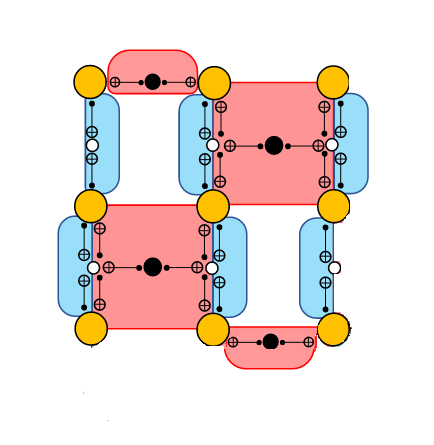
Figure 1. Distance 3 heavy hexagon code encoding one logical qubit. The yellow vertices denote the data qubits, the white vertices the flag qubits and the black vertices represent the ancilla to measure the $X$-type gauge generators (red areas) and the $Z$-type gauge generators (blue areas). The product of the two $Z$-type gauge generators at each white face forms a $Z$-type stabilizer (chamberland2020topological, ).

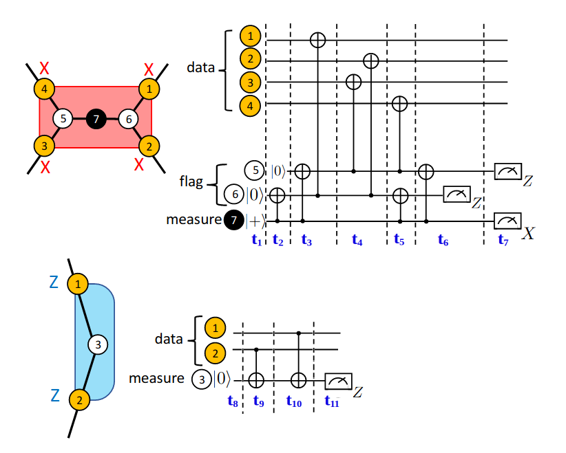
Figure 2. Circuits for the $X$ and $Z$-type parity measurements in the heavy hexagon code where $t_{i}$ denotes the $i^{th}$ time step. Two flag qubits (white circles) are used to measure the weight-four $X$-type gauge generators. One flag qubit is used to measure the weight-two $Z$-type gauge generators (chamberland2020topological, ).

2.1. Heavy Hexagon Code

The heavy hexagon code encodes a logical qubit over a heavy hexagonal lattice. As qubits are placed on both the vertices and edges of the lattice, the term heavy is used. This is a combination of degree-2 and degree-3 qubits hence there is a huge improvement in terms of average qubit degree in comparison with surface code structure which has qubits of degree-4 (chamberland2020topological, ). In Fig 1, the layout for a distance-3 heavy hexagon code encoding one logical qubit and in Fig. 2 an illustration of the circuits for measuring the $X$ and $Z$-type gauge generators is given (chamberland2020topological, ) . A single error correction cycle requires 11 time steps (7 for $X$ and 4 for $Z$) as shown in Fig. 2.

The heavy hexagon code is a combination of surface code and subsystem code (Bacon Shor code) (chamberland2020topological, ). A subsystem code is defined by a set of gauge operators $G$, such that $\forall$ $g\in G$, $\ket{\psi}$ is equivalent to $g\ket{\psi}$, i.e., $\ket{\psi}\equiv g\ket{\psi}$. In other words, a codespace in a subsystem code consists of multiple equivalent subsystems. A gauge operator takes a codeword to an equivalent subsystem. The product of multiple gauge operators form a stabilizer, which keeps the codeword unchanged.

2.1.1. Gauge generators

The gauge group for the heavy hexagon code (chamberland2020topological, ) is given in Eq. (1) . Here, the row and column indices of the data qubits $i,j=1,2,\ldots,d-1,m=(1,2,\ldots,(d-1)/2)$, with the constraint that in case of weight-4 gauge operators, $i+j$ is even for the second term.

(1) $$G=\langle Z_{i,j}Z_{i+1,j},\leavevmode\nobreak\ X_{i,j}X_{i,j+1}X_{i+1,j}X_{i+1,j+1},\leavevmode\nobreak\ X_{1,2m-1}X_{1,2m},\leavevmode\nobreak\ X_{d,2m}X_{d,2m+1}\rangle$$

For the rest of the paper, we call each of the operators in Eq. (1) as gauge generator. In Fig. 3, the $Z$ and $X$-type gauge generators used to correct bit and phase errors, are indicated in blue and red respectively. One or more generators can be used to form a gauge operator.

For example: here $d=5$, $i,j=1,2,3,4;m=1,2$, with the constraint that $i+j$ is even for the second term. Therefore there are 20 $Z$ gauge generators (of the form $Z_{i,j}Z_{i+1,j}$) in Fig. 3:

• $Z_{1,1}Z_{2,1}\rightarrow$ first row first column (top left) blue semicircle,

• $Z_{2,1}Z_{3,1}\rightarrow$ second row first column blue semicircle,
  ⋮

• $Z_{4,5}Z_{5,5}\rightarrow$ last row last column blue semicircle, marked as $Z$ gauge.

The 8 $X$ gauge generators (of the form $X_{i,j}X_{i,j+1}X_{i+1,j}X_{i+1,j+1}$ represented as red squares) in Fig. 3 are:

• $X_{1,2}X_{1,3}X_{2,2}X_{2,3}\rightarrow$ first row second column red square,

• $X_{1,4}X_{1,5}X_{2,4}X_{2,5}\rightarrow$ first row fourth column red square,
  ⋮

• $X_{3,4}X_{3,5}X_{4,4}X_{4,5}\rightarrow$ third row second column red square, marked as $X$ gauge.

The 2 $X$ gauge generators (of the form $X_{1,2m-1}X_{1,2m}$, represented as red semicircles) in Fig. 3 are:

• $X_{1,1}X_{1,2}\rightarrow$ first row first column (top left) red semicircle,

• $X_{1,3}X_{1,4}\rightarrow$ first row third column red semicircle.

The 2 $X$ gauge generators (of the form $X_{d,2m}X_{d,2m+1}$ represented as red semicircles) in Fig. 3 are:

• $X_{5,2}X_{5,3}\rightarrow$ fifth row second column red semicircle,

• $X_{5,4}X_{5,5}\rightarrow$ fifth row fifth column red semicircle (bottom right).

Hence there are a total of 12 $X$ gauge generators in Fig. 3. The number of possible gauge operators is exponential in $d$, thereby syndrome decoding poses a computational challenge.

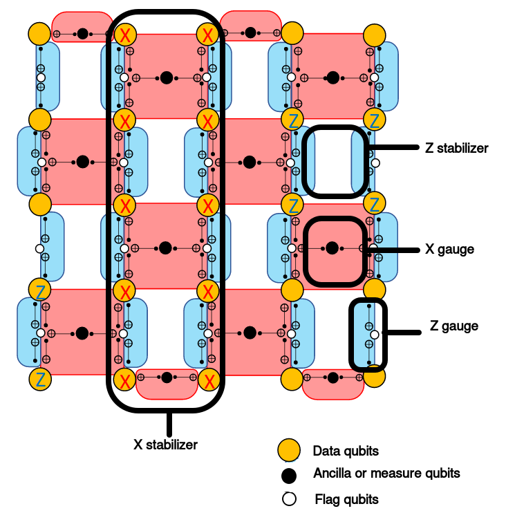
Figure 3. Distance 5 heavy hexagon code Gauge generators: weight-four $X$-type in the plaquetes, weight-two $X$-type on the upper and lower boundaries, and weight-two $Z$-type. Stabilizer operators: a two-column vertical strip with $X$-type, weight-four $Z$-type in the plaquetes, and weight-two $Z$-type on the left and right boundaries. (chamberland2020topological, ).

2.1.2. Stabilizers

The stabilizer group of the heavy hexagon code is shown in Eq. (2) (chamberland2020topological, ). Here, $Z_{i,j}Z_{i,j+1}Z_{i+1,j}Z_{i+1,j+1}$ is a weight-four stabilizer, similar to that in surface code. The measurement outcome of one such stabilizer is the product of the measured eigenvalues of the two weight-two gauge generators $Z_{i,j}Z_{i+1,j}$ and $Z_{i,j+1}Z_{i+1,j+1}$, with the constraint that $i+j$ even for the first term..

(2) $$S=\langle Z_{i,j}Z_{i,j+1}Z_{i+1,j}Z_{i+1,j+1},\leavevmode\nobreak\ Z_{2m-1,d}Z_{2m,d},\leavevmode\nobreak\ Z_{2m,1}Z_{2m+1,1},\leavevmode\nobreak\ \Pi_{i}X_{i,j}X_{i,j+1}\rangle$$

Therefore for $d=5$, the 8 $Z$ stabilizers (of the form $Z_{i,j}Z_{i,j+1}Z_{i+1,j}Z_{i+1,j+1}$) in Fig. 3 are:

• $Z_{1,1}Z_{1,2}Z_{2,1}Z_{2,2}\rightarrow$ first row first column white square,
  ⋮

• $Z_{2,4}Z_{2,5}Z_{3,4}Z_{3,5}\rightarrow$ second row fourth column blue semicircle marked as $Z$ stabilizer.

The 2 $Z$ stabilizers (of the form $Z_{2m-1,d}Z_{2m,d}$) in Fig. 3 are:

• $Z_{1,5}Z_{2,5}\rightarrow$ first row fifth column blue semi circle,

• $Z_{3,5}Z_{4,5}\rightarrow$ which is the third row fifth column blue semi circle.

The 2 $Z$ stabilizers (of the form $Z_{2m,1}Z_{2m+1,1}$) in Fig. 3 are:

• $Z_{2,1}Z_{3,1}\rightarrow$ second row first column blue semi circle,

• $Z_{4,1}Z_{5,1}\rightarrow$ fourth row first column blue semi circle.

There are a total of 12 $Z$ stabilizers in Fig. 3. The 4 $X$ stabilizers (of the form $\Pi_{i}X_{i,j}X_{i,j+1}$) are:

• $X_{1,1}X_{1,2}X_{2,1}X_{2,2}X_{3,1}X_{3,2}X_{4,1}X_{4,2}X_{5,1}X_{5,2}\rightarrow$ the vertical strip of the first two columns,

• $X_{1,2}X_{1,3}X_{2,2}X_{2,3}X_{3,2}X_{3,3}X_{4,2}X_{4,3}X_{5,2}X_{5,3}\rightarrow$ the vertical strip of the second two columns marked as $X$ stabilizer,
  ⋮

For QECCs which are not subsystem codes, such as (Shor:1997:PAP:264393.264406, ; PhysRevLett.77.793, ), $n-k$ stabilizers for an $n$-qubit QECC can correct upto $k$ errors. On the other hand, subsystem codes have fewer number of stabilizers (bacon2006operator, ). Decoding of error is anyway not a one-to-one mapping. Nevertheless, for subsystem codes, this becomes an even more difficult problem since the decoder needs to identify between equivalent errors. This has motivated us here to design an ML based decoder, along with two efficient algorithms to identify equivalence classes for all possible errors to enhance the efficiency of the decoder.

2.2. Machine Learning based decoding

Minimum Weight Perfect Matching algorithm (MWPM) has been used for decoding the heavy hexagonal code (chamberland2020topological, ). Machine learning based decoders have been shown to outperform MWPM for surface codes (baireuther2018machine, ; varsamopoulos2017decoding, ; krastanov2017deep, ; varsamopoulos2019comparing, ; bhoumik2022ml, ). In this article we have designed ML based decoders for the heavy hexagonal code, and have shown that the subsystem property of this code leads to even more efficient decoding than surface code. We elaborate on those properties in Sec. 4 below.

2.2.1. Motivation for using Machine Learning based syndrome decoder

Topological codes, such as surface code and heavy hexagonal code, are degenerate, i.e., $\exists$ errors $e_{1}\neq e_{2}$ such that $e_{1}\ket{\psi}=e_{2}\ket{\psi}$, where $\ket{\psi}$ is the codeword (fowler2012towards, ). This leads to failure of any decoder in distinguishing between such errors $e_{1}\neq e_{2}$. Nevertheless, that does not always lead to a logical error (bhoumik2022ml, ). Usually the decoder incorporates logical errors when it fails to distinguish between $\lfloor\frac{d-1}{2}\rfloor$ and $\lceil\frac{d+1}{2}\rceil$ errors (fowler2012towards, ).

Classical algorithms, such as Minimum Weight Perfect Matching (MWPM) (edmonds_1965, ), used for decoding topological error correcting codes (fowler2012towards, ; chamberland2020topological, ) aim to find the minimum number of errors that can recreate the obtained error syndrome without considering the probability of various errors. Therefore, such a decoder is largely vulnerable to the above discussed drawback. Furthermore, the time complexity of MWPM grows as $\mathcal{O}(N^{4})$ where $N$ is the number of qubits.

In order to overcome these drawbacks, ML techniques have been applied to learn the probability of error in the system and propose the best possible correction accordingly (baireuther2018machine, ; varsamopoulos2017decoding, ; krastanov2017deep, ; varsamopoulos2019comparing, ; bhoumik2022ml, ) with comparatively lower time complexity (varsamopoulos2019comparing, ). Broadly speaking, ML can learn the probability of error and predict which one of the $\lfloor\frac{d-1}{2}\rfloor$ and $\lceil\frac{d+1}{2}\rceil$ errors is more likely.

3. Design methodology of the ML based decoder for heavy hexagonal code

Artificial neural networks (ANN) are brain-inspired systems which are intended to replicate the way that we humans learn and they are one of the most widely used tools in ML. Neural networks consist of one input layer, one output layer, and a few hidden layers consisting of units that transform the input into an intermediate form from which the output layer can find patterns - typically too complex for a human programmer to teach the machine. The time complexity of training a neural network with $N$ inputs, $M$ outputs and one hidden layer with $L$ nodes is $\mathcal{O}((M+N)\cdot L)$. In this paper we are using feed forward neural network for decoding heavy hexagonal code of distance 3, 5, and 7 .

For application of ML techniques to decoding, we first reduce the decoding problem to classification, a well-studied problem in machine learning. Classification is the process of predicting the class of given data points. Classes are also known as labels. Classification is the task of approximating a mapping function $f$ from input variables $x$ to discrete output variables $y$. The methodology to map heavy hexagon code is similar with surface code which has already been discussed in detail in (bhoumik2022ml, ).

A distance $d$ heavy hexagon code has

• $(d^{2}-1)/2$ syndrome bits in case of bit flip error – refer to $Z$ stabilizers in Fig. 3.

• $d-1$ syndrome bits in case of phase flip error – refer to $X$ stabilizers in Fig. 3.

This syndrome is the input data to the ML model. The label of the ML model is the erroneous data qubit of the heavy hexagon code structure hence it has $d^{2}$ qubits in each entry. Now our problem of interest is mapped into a multilabel multiclass classfication problem because there are:

• multiple classes - ${2^{d^{2}}}$;

• each class label consists of multiple bits ($d^{2}$).

We train a feed forward neural network where the input layer is the syndrome (measured ancilla qubits) and the output layer denotes the types of errors along with the physical data qubit where each error has occurred.

4. Error class minimization methods for heavy hexagonal codes

As mentioned in earlier sections, the heavy hexagon code is a subsystem code. A subsystem code is defined by a set of gauge operators $G$, forming a group (called the gauge group) (bacon2006operator, ). This group defines an equivalence relation $\equiv$ over the state space defined by $\forall$ $g\in G$, $\ket{\psi}\equiv g\ket{\psi}$. In other words, in a subsystem code, the entire codespace is divided into equivalent classes called subsystems. A gauge operator takes the codeword to an equivalent subsystem. A stabilizer, which is a product of one or more gauge operators, keeps the codeword unchanged.

The subsystem code property asserts that if $\Pi_{j}g_{j}$ denotes the product of one or more gauge operators, then

• if an error $e=\Pi_{j}g_{j}$, it can be safely ignored since the system transforms to an equivalent subsystem;

• if for two errors $e_{1}$ and $e_{2}$, $e_{2}=e_{1}\Pi_{j}g_{j}$, then $e_{2}$ can be considered as $e_{1}$ since they take the state to equivalent erroneous subsystems,

In this paper, the second scenario is termed as gauge equivalence, which provides significant advantage in designing decoders based on ML.

ML based decoding being a classification problem, for each of $\sigma_{x}$ or $\sigma_{z}$ error, an ML decoder for a distance $d$ heavy hexagon code (which has $d^{2}$ number of qubits) is a classification amongst the $2^{d^{2}}$ possible errors which we call as an error class henceforth. However, since the heavy hexagonal code is a subsystem code, $\exists$ $i\neq j$ such that $Q_{i}$ is gauge equivalent to $Q_{j}$. For the rest of the paper, if $\ket{\psi}\equiv\Pi_{j}g_{j}\ket{\phi}$, where $\Pi_{j}g_{j}$ denotes the product of one or more gauge operators $g_{j}$, then we write $\ket{\psi}\equiv\ket{\phi}$ modulo $(\Pi_{j}g_{j})$.

For example, in Fig 4 there are 4 $X$-gauge generators $G1,G2,G3,G4$, 6 $Z$-gauge generators $g1,g2,g3,g4,g5,g6$ and the qubits are $Q1,Q2,...,Q9$. If $\ket{\psi}$ is the codeword, then,

• $X_{4}X_{7}X_{8}\ket{\psi}\equiv X_{5}\ket{\psi}$ modulo ($G_{3}$), where $X_{k}$ denotes bitflip error on qubit $Q_{k}$.

• $Z_{7}\ket{\psi}\equiv Z_{1}\ket{\psi}$ modulo ($g_{4}g_{1}$), where $Z_{k}$ denotes phaseflip error on qubit $Q_{k}$.

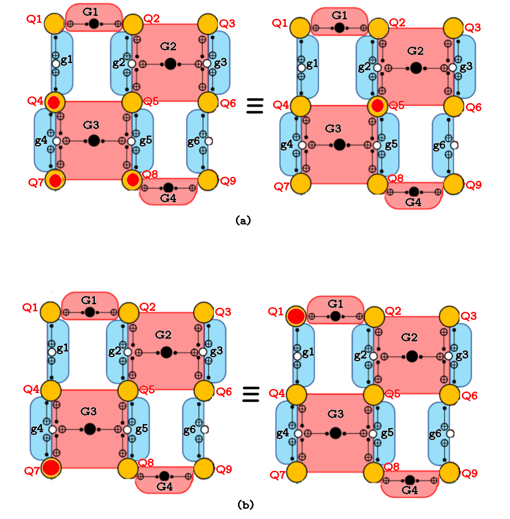
Figure 4. (a) $X$ gauge equivalence (b)$Z$ gauge equivalence

The notion of gauge equivalent error strings creates a problem for machine learning based decoding since the problem of mapping syndromes to error strings is not well defined because there can be multiple Pauli error strings which are gauge equivalent having the same syndrome. In order to remedy the above, we identify a representative element from each such a error class. Every error string in the training data is mapped to the representative element of its corresponding class. Next, can we reduce the number of error classes? Reduction in the number of error classes implies a classification problem with fewer classes, which helps in improving the performance further for the ML model. We now formally define the criteria for two qubits to belong to the same error class.

Lemma 4.1.

Given a codeword $\ket{\psi}$ such that $\ket{\psi}\equiv\Pi_{j}g_{j}\ket{\psi}$, where $\Pi_{j}g_{j}$ implies the product of one or more gauge operators $g_{j}$, any error $e$ acting on the codeword is equivalent to $e(\Pi_{j}g_{j})$.

Proof.

Consider an error $e$ acting on the codeword $\ket{\psi}$ such that $\ket{\psi}\equiv\Pi_{j}g_{j}\ket{\psi}$. Therefore,

$$e\ket{\psi} \equiv e\Pi_{j}g_{j}\ket{\psi}\Rightarrow e\equiv e(\Pi_{j}g_{j})$$

∎

Lemma 4.1 implies that it is acceptable to consider $e$ and $e(\Pi_{j}g_{j})$ as the same error class. Such equivalence leads to a set of error classes whose cardinality is $<2^{d^{2}}$, where errors in the same class act equivalently on the codeword. Therefore, it is not necessary to distinguish between the errors in the same error class. It suffices to identify the error class only.

Henceforth we propose two methods to find gauge equivalence and determine the error classes for the heavy hexagonal code, namely search based equivalence and rank based equivalence.

4.1. Minimizing error classes for bit flip using search based gauge equivalence

The heavy hexagonal code is similar to surface code (bravyi1998quantum, ) and Bacon-Shor code (bacon2006operator, ) for bit flip and phase flip errors respectively (chamberland2020topological, ). We have already discussed that the heavy hexagonal code is a subsystem code. We employ this property to modify our training dataset into another equivalent training dataset with fewer class labels. In this subsection we provide an algorithm to obtain the equivalent training dataset, having fewer class labels for bitflip errors.

In order to provide the Algorithm, we first discuss in Lemma 4.2 the reduction in the number of error classes obtained due to the subsystem property. Since multiple errors can fall under the same class, we require a class representative, which we discuss next, followed finally by the Algorithm to obtain such equivalence.

Lemma 4.2.

The total number of error classes for bit flip error in any distance $d$ heavy hexagonal code is $2^{\frac{d^{2}+1}{2}}$.

Proof.

For a distance $d$ heavy hexagonal code, the total number of data qubits is $d^{2}$ and the number of $X$ gauge generators is $\frac{d^{2}-1}{2}$. Therefore, the total possible combinations of these $X$ gauge operators is $2^{\frac{d^{2}-1}{2}}$. For each of these operators $g$, any error $e\equiv e.g$. Therefore, $e$ and $e.g$ belong to the same error class. The total number of error classes, thus, is

$$2^{d^{2}}/2^{\frac{d^{2}-1}{2}}=2^{\frac{d^{2}+1}{2}}$$

∎

Therefore, we roughly have a square root reduction in the number of error classes. In Table 1 we show the reduction in the number of error classes for codes of distance 3, 5 and 7 due to this equivalence. Since multiple errors fall under the same error class, it is necessary to choose a class representative.

Table 1. Number of class labels before and after gauge equivalence

Code distance	Before equivalence	After equivalence
3	$2^{9}$	$2^{5}$
5	$2^{25}$	$2^{13}$
7	$2^{49}$	$2^{25}$

Choice of class representative: If errors $e_{1},\ldots,e_{k}$ belong to the same error class $\mathcal{E}$, then we choose a class representative $e_{i}\in\mathcal{E}$ which will be considered as the error on the codeword for any error $e\in\mathcal{E}$ occurring on the codeword. To provide an example, it can be verified that bit flip errors on qubits 4, 7 and 8 produce the same syndrome as that on 5 (Refer Fig. 4). But for training the ML decoder, we shall choose the second one as the common label for both since it has a lower weight. However, simply considering the weight of the errors is not sufficient to obtain a class representative. For example, bit errors on qubits 1 and 2 lead to the same syndrome, and both of these errors have weight 1. Therefore, we use the method of lexicographic minima to obtain the class representative.

For finding the lexicographic minima, we assume the set of qubits in the codeword to be a $1\times d^{2}$ array, where the values of the position $k$ is 1 if an error occurred on qubit $k$, or 0 otherwise. In this representation, the previously mentioned bit flip error on qubits 4, 7 and 8 will take the notation $e=[000100110]$. For each error class $\mathcal{E}$, we choose that error $e$ as the class representative for which $\displaystyle\sum_{i\in pos}2^{i}*Arr[i]$ is minimum, where $Arr$ denote the array representation of errors. For example, in a distance 3 heavy hexagonal code, bit flip error on qubits 1 and 2 respectively will have the representations $e_{1}=[100000000]$ and $e_{2}=[010000000]$. We can see that $X$-operator on qubits 1 and 2 form an $X$-gauge operator, say $g_{1}$. Hence applying $g_{1}$ on $e_{1}$ gives us $e_{2}$, and vice-versa. So $e_{1}$ and $e_{2}$ belongs to same error class $\mathcal{E}$. Now to choose the class label for $\mathcal{E}$ we will choose the lexicographic minimum (LM) $\displaystyle\sum_{i\in pos}2^{i}*Arr[i]$, which is $LM_{1}=2^{1}\times 1+2^{2}\times 0+2^{3}\times 0+...+2^{9}\times 0=2$ for $e_{1}$ and $LM_{2}=2^{1}\times 0+2^{2}\times 1+2^{3}\times 0+...+2^{9}\times 0=4$ for $e_{2}$. Since $LM_{1}<LM_{2}$ hence $e_{1}$ will be the class representative.

Now, in Algorithm 1 we provide the algorithm to find the equivalent for each error $e$ in the training dataset, and depict its runtime and space in Lemmata 4.4 and  4.5.

Algorithm 1 Search Based Gauge equivalence minimization for bit flip

0:  List of $X$-gauge operators = $G_{x}$, distance of the code = $d$, error string $e$ .

0:  Error string $MinWeightEquiv$ which is equivalent to $e$ .

1:  $MinWeightEquiv=e$

2:  $MinWeight=\displaystyle\sum_{k\in d^{2}}2^{k}*e[k]$

3:  for all  $g_{x}\in G_{x}$ do

4:     $GaugeEquiv=e\oplus g_{x}$

5:     $weight_{GE}$ = $\displaystyle\sum_{k\in d^{2}}2^{k}*GaugeEquiv[k]$

6:     if $MinWeight>weight_{GE}$ then

7:        $MinWeight=weight_{GE}$

8:        $MinWeightEquiv=GaugeEquiv$

9:     end if

10:  end for

11:  return $MinWeightEquiv$

Theorem 4.3.

Given a training sample $e$ in which each qubit may be error free or has bit flip error only, its corresponding gauge equivalent minima $e_{min}\equiv e$ can be computed, according to Algorithm 1 in $\mathcal{O}(N\cdot d^{2}\cdot 2^{d^{2}/2})$ using $\mathcal{O}(d^{2}\cdot 2^{\frac{d^{2}-1}{2}}+N.d^{2})$ space, where $d$ is the distance of the code and $N$ is the number of training samples.

Proof.

We prove this theorem in two steps. The proofs for time and space complexity are shown individually in Lemmata 4.4 and  4.5 respectively. ∎

Lemma 4.4.

Given a training sample $e$ in which each qubit may be error free or has bit flip error only, its corresponding gauge equivalent minima $e_{min}\equiv e$ can be computed, according to Algorithm 1, in $\mathcal{O}(N\cdot d^{2}\cdot 2^{d^{2}/2})$, where $d$ is the distance of the code and $N$ is the number of training samples.

Proof.

From Lemma 4.2 total possible combinations of the $X$ gauge operators is $2^{\frac{d^{2}-1}{2}}$. Each of line number 2, 5, and 6 of Algorithm 1, requires bitwise operation over the length of the error string which is $d^{2}$.

Finding the minimum weight among gauge equivalent errors requires constant time. Therefore, the runtime for each training sample is $d^{2}+d^{2}\cdot 2^{\frac{d^{2}-1}{2}}+c$, where $c$ is a constant, leading to a time complexity of $\mathcal{O}(d^{2}\cdot 2^{d^{2}/2})$. Hence , the total runtime of Algorithm 1 to find the gauge equivalence for the entire training dataset consisting of $N$ samples is $\mathcal{O}(N\cdot d^{2}\cdot 2^{d^{2}})$. ∎

We consider our dataset consists of $N$ training samples, where each sample can consist of 0 or more errors.

Lemma 4.5.

Given a training sample $e$ in which each qubit may be error free or has bit flip error only, to compute its corresponding gauge equivalent minima $e_{min}\equiv e$ according to Algorithm 1 has space complexity of $\mathcal{O}(d^{2}\cdot 2^{\frac{d^{2}-1}{2}}+N.d^{2})$, where $d$ is the distance of the code and $N$ is the number of training samples.

Proof.

From Lemma 4.2, total possible combinations of the $X$ gauge operators is $2^{\frac{d^{2}-1}{2}}$. Each gauge operator consists of $d^{2}$ bits. Hence the total space required to store all the gauge operators is $\mathcal{O}(d^{2}\cdot 2^{\frac{d^{2}-1}{2}})$. Furthermore, the entire training dataset, consisting of $N$ samples, must be stored as well. Each training data requires $\mathcal{O}(d^{2})$ space, leading to an overall requirement of $\mathcal{O}(N.d^{2})$. Therefore, the total space needed for Algorithm 1 is $\mathcal{O}(d^{2}\cdot 2^{\frac{d^{2}-1}{2}}+N.d^{2})$. ∎

Table 2. Number of class labels before and after gauge equivalence in case of phase flip

Code distance	Before equivalence	After equivalence
3	$2^{9}$	$2^{3}$
5	$2^{25}$	$2^{5}$
7	$2^{49}$	$2^{7}$

Instead of calculating all possible combination of $X$ gauge operators beforehand, if we calculate them on the go, then the space complexity can be reduced to $\mathcal{O}(d^{4}+N.d^{2})$. However, for such an algorithm, the entire set of gauge operators need to be generated for every training sample, leading to a time complexity of upto $\mathcal{O}(N\cdot d^{4}\cdot 2^{d^{2}/2})$.

4.2. Minimizing error classes for phase flip using search based gauge equivalence

In this subsection, we show the similar studies for phase flip error as we did for bit flip error in the previous subsection. The Bacon-Shor structure of phase stabilizers allow for more equivalent subsystems, leading to fewer error classes. We first depict this equivalence for phase errors in Lemma 4.6, and provide the algorithm to find the phase equivalence in Algorithm 2.

Lemma 4.6.

For any column $1\leq j\leq d$ of qubits, where $Z_{i,j}$ denotes the phase operator on $i^{th}$ qubit of the $j^{th}$ column, where $1\leq i\leq d$, $Z_{i,j}$ is gauge equivalent to $Z_{1,j}$.

Proof.

We prove this by induction.

Base Case: If a phase error occurs on the first qubit of any column of qubits $j$, then it is trivially equivalent to $Z_{1,j}$.

Induction Hypothesis: Let for some $1\leq m<d$, $Z_{m,j}$ is gauge equivalent to $Z_{1,j}$.

Induction Step: Consider a phase operator $Z_{m+1,j}$. We note that for any $1\leq m<d$, $\exists$ $Z$ gauge operator $g_{m,m+1,j}$ = $Z_{m,j}Z_{m+1,j}$. Therefore, $Z_{m+1,j}$ is gauge equivalent to $(Z_{m+1,j})\cdot(Z_{m,j}Z_{m+1,j})=Z_{m,j}$ . Since from induction hypothesis, $Z_{m,j}$ is gauge equivalent to $Z_{1,j}$, we have $Z_{m+1,j}$ is also gauge equivalent to $Z_{1,j}$. ∎

Corollary 4.7.

There are $2^{d}$ non-equivalent error classes for phase flip errors.

Proof.

This corollary follows directly from Lemma 4.6. Since for a particular qubit column $j$, $q_{j}^{i}$ is gauge equivalent to $q_{j}^{1}$ for any $1\leq i\leq d$, each qubit column corresponds to a possible error class. There are $d$ many qubit columns. Therefore, for phase flip errors, there are $2^{d}$ non-equivalent error classes. ∎

Now, in Algorithm 2 we provide the algorithm to find the equivalent for each error $e$ in the training dataset, and depict its runtime and space in Lemmata 4.9 and  4.10.

Algorithm 2 Search Based Gauge equivalence minimization for phase flip

0:  Distance of the code = $d$, error string $e$ .

0:  Error string $MinWeightEquiv$ which is equivalent to $e$ .

1:  for $j=d$ to $d^{2}-1$ do

2:     $l=j\%d$

3:     $e[l]=e[l]\oplus e[j]$

4:  end for

5:  $MinWeightEquiv$ = $e$

6:  return $MinWeightEquiv$

Theorem 4.8.

Given a training sample $e$ in which each qubit may be error free or has phase flip error only, its corresponding gauge equivalent minima $e_{min}\equiv e$ can be computed, according to Algorithm 2 in $\mathcal{O}(d^{2})$ using $\mathcal{O}(N.d^{2})$ space, where $d$ is the distance of the code and $N$ is the number of training samples.

Proof.

We prove this theorem in two steps. The proofs for time and space complexity are shown individually in Lemmata 4.9 and  4.10 respectively. ∎

Lemma 4.9.

Given a phase flip error $e$, its corresponding gauge equivalent minima $e_{min}\equiv e$ can be computed, according to Algorithm 2 in $\mathcal{O}(d^{2})$, where $d$ is the distance of the code.

Proof.

Lemma 4.6 asserts that for each of the column of the heavy hexagonal code, any phase error on a qubit in that column is gauge equivalent to the phase error on the top most qubit of that column. Therefore, Algorithm 2 starts from the second row of the heavy hexagonal structure, leaving aside the topmost row (length $d$) which consists of the 1st qubits of each column. Each of line number 2 and 3 of Algorithm 2, requires a constant time operation for $d^{2}-d$ number of strings. Therefore, the total runtime of Algorithm 2 is $c\cdot(d^{2}-d)$, where $c$ is a constant, leading to a time complexity of $\mathcal{O}(d^{2})$. ∎

Therefore, we obtain a quadratic reduction in the number of error classes for both, bit flip and phase flip errors but the reduction is much higher in case of phase flip errors.

Lemma 4.10.

Given a phase flip error $e$, to compute its corresponding gauge equivalent minima $e_{min}\equiv e$, according to Algorithm 2 has a space complexity of $\mathcal{O}(N.d^{2})$ where $d$ is the distance of the code, and $N$ number of training samples.

Proof.

In order to store $N$ number of training samples we need $\mathcal{O}(N.d^{2})$ amount of space. Therefore, the total space needed for Algorithm 2 is $\mathcal{O}(N.d^{2})$ . ∎

We observed that the time complexity for bit flip error is $\mathcal{O}(d^{2}\cdot 2^{d^{2}})$ and for phase flip $\mathcal{O}(d^{2})$. In the next subsection we are proposing a method named rank based gauge equivalence minimization which can further reduce the time complexity for bitflip errors.

4.3. Minimizing error classes for bit flip using rank based gauge equivalence minimization

In this subsection we provide a more time-efficient algorithm to find the gauge equivalence for bit flip errors. This algorithm relies on finding the rank of the matrix created using the gauge generators, as its column. The rank of a matrix denotes the number of linearly independent columns of that matrix (strang2006linear, ). We denote $M=[GEN_{x}]$ to be the matrix generated by using the $X$-gauge generators as its column. Since each gauge generators are linearly independent, $M$ will exhibit full rank, i.e., the number of gauge generators $(d^{2}-1)/2$. Now, if two errors $e_{i}$ and $e_{k}$ are equivalent, then $e_{k}$ can be written as $(\Pi_{j}g_{j})e_{i}$. In other words, if we form another matrix $M^{\prime}=[GEN_{x},e_{i}-e_{k}]$, where $e_{i}-e_{k}$ is the last column of $M^{\prime}$, then $M$ and $M^{\prime}$ will have the same rank if $e_{i}$ and $e_{k}$ are equivalent. We use this notion to find the gauge equivalence for bit flip errors faster than Algorithm 1.

In Algorithm 3 we provide the algorithm to find the equivalent for each error $e$ in the training dataset, and depict its time and space complexities in Lemmata 4.12 and  4.13 respectively.

Algorithm 3 Rank Based Gauge equivalence minimization for bit flip

0:  List of $X$-gauge generators = $GEN_{x}$, distance of the code = $d$, List of all errors in the dataset $E[1:j]$ which consists $e_{1},e_{2},...,e_{j}$.

0:  Error string $MinWeightEquiv$ which is equivalent to $e_{j}$.

1:  $MinWeightEquiv={e_{j}}$

2:  $MinWeight=\displaystyle\sum_{k\in d^{2}}2^{k}*{e_{j}}[k]$

3:  $M=[GEN_{x}]$ where each $GEN_{x}$, $0\leq x\leq(d^{2}-1)/2$ forms a column of $M$.

4:  Calculate the rank $M$

5:  for all $e=e_{1}$ to $e_{j-1}$ do

6:     if $syndrome(e_{j})==syndrome(e)$ then

7:        Form a matrix $M^{\prime}$ by appending $e_{j}-e$ as the last column of $M$

8:        Calculate the rank of $M^{\prime}$

9:        if $Rank(M)==Rank(M^{\prime})$  then

10:           $weight_{GE}$ = $\displaystyle\sum_{k\in d^{2}}2^{k}*e[k]$

11:           if $MinWeight>weight_{GE}$ then

12:              $MinWeight=weight_{GE}$

13:              $MinWeightEquiv=e$

14:           end if

15:        end if

16:     end if

17:  end for

18:  Return $MinWeightEquiv$

Theorem 4.11.

Given a training sample $e$ in which each qubit may be error free or has bit flip error only, its corresponding gauge equivalent minima $e_{min}\equiv e$ can be computed, according to Algorithm 3 in $\mathcal{O}(N^{2}\cdot d^{4})$ using $\mathcal{O}(d^{4}+N.d^{2})$ space, where $d$ is the distance of the code and $N$ is the number of training samples.

Proof.

We prove this theorem in two steps. The proofs for time and space complexity are shown individually in Lemmata 4.12 and  4.13 respectively. ∎

Lemma 4.12.

Given a bit flip error $e$, its corresponding gauge equivalent minima $e_{min}\equiv e$ can be computed, according to Algorithm 3 in $\mathcal{O}(N^{2}\cdot d^{4})$ where $d$ is the distance of the code and entire dataset consists of $N$ errors.

Proof.

According to Algorithm 3, both of line 2, and 10 requires bitwise operation over the length of the error string which is $d^{2}$ and computation of the syndrome equality in line 6 requires bitwise operation over the length of the syndrome string which is $(d^{2}-1)/2$. There are $d^{2}$ number of data qubits and the number of gauge generators is $(d^{2}-1)/2$. Furthermore, calculation of rank of an $m\times n$ matrix is $\mathcal{O}(m\cdot n)$ (cormen2022introduction, ). Therefore calculating the rank of matrix M of size ($d^{2}\times(d^{2}-1)/2)$), in line 4, has a running time of $\mathcal{O}(d^{4})$. Hence for a particular error $e_{j}$, time required to calculate the gauge equivalence is $\sum_{i=1}^{j-1}\mathcal{O}(d^{4}+d^{2})$ = $\mathcal{O}((d^{4}+d^{2})\cdot j)$.
Hence for the entire dataset consisting of $N$ errors, the runtime of Algorithm 3 is

$$\mathcal{O}((d^{4}+d^{2})\cdot\sum_{j=1}^{N}j) = \mathcal{O}(N^{2}\cdot(d^{4}+d^{2}))$$

$$= \mathcal{O}(N^{2}\cdot d^{4})$$

∎

Lemma 4.13.

Given a bit flip error $e$, to compute its corresponding gauge equivalent minima $e_{min}\equiv e$, according to Algorithm 3 has space complexity of $\mathcal{O}(d^{4}+N.d^{2})$ where $d$ is the distance of the code and $N$ is the number of training samples.

Proof.

For a distance $d$ heavy hexagonal code, the total number of data qubits is $d^{2}$ and the number of $X$ gauge generators is $\frac{d^{2}-1}{2}$. Each of the gauge generators consists $d^{2}$ bits. Hence, to store the generator matrix $M$, the space needed is $d^{2}\cdot(d^{2}-1)/2$. To store the appended matrix $M^{\prime}$, $d^{2}\cdot((d^{2}-1)/2+1)$ space is needed and to store $N$ number of training samples, $N\cdot d^{2}$ space is needed. Hence, the total amount of space needed is $d^{2}\cdot(d^{2}-1)/2+d^{2}\cdot((d^{2}-1)/2+1)+N\cdot d^{2}$ leading to a space complexity of $\mathcal{O}(d^{4}+N.d^{2})$.

∎

A natural question, therefore, is when it is better to use rank based equivalence over the search based one. We provide the criteria in Corollary 4.14.

Corollary 4.14.

Rank based equivalence method finds gauge equivalence faster than the search based method when $N\cdot d^{2}\cdot 2^{d^{2}}\geq c_{\cdot}(N^{2}\cdot d^{4})$, where $d$ is the distance of the code, $N$ is the number of training samples, and $c$ is some constant.

Proof.

According to Lemma 4.4, given a bit flip error $e$, its corresponding gauge equivalent minima $e_{min}\equiv e$ can be computed, according to Algorithm 1, in $\mathcal{O}(d^{2}\cdot 2^{d^{2}})$, where $d$ is the distance of the code. Hence the total time required to find the gauge equivalence for the entire training dataset consisting of $N$ samples is $\mathcal{O}(N\cdot d^{2}\cdot 2^{d^{2}})$. According to 4.12 given a bit flip error $e$, its corresponding rank based gauge equivalent minima $e_{min}\equiv e$ can be computed, according to Algorithm 3 in $\mathcal{O}(N^{2}\cdot d^{4})$ where $d$ is the distance of the code and entire dataset consists of $N$ errors. Hence we will use rank based gauge minimization only when,

$$\mathcal{O}(N\cdot d^{2}\cdot 2^{d^{2}}) \geq \mathcal{O}(N^{2}\cdot d^{4})$$

$$\Rightarrow c_{1}\cdot N\cdot d^{2}\cdot 2^{d^{2}} \geq c_{2}N^{2}\cdot d^{4}$$

$$\Rightarrow N\cdot d^{2}\cdot 2^{d^{2}} \geq c_{2}N^{2}\cdot d^{4}$$

where $c=\frac{c_{2}}{c_{1}}$ is a constant. ∎

From corollary 4.14 we find the condition for which the rank based minimization requires lesser time. We have empirically tested that for $d>3$ rank based minimization is faster than its search based counterpart. But this improvement is obtained only for bit flip error. Hence for phase flip errors we have used only search based gauge equivalence minimization throughout the result section.

5. Simulation Results

5.1. Noise models

5.1.1. Bit flip

Given a quantum state $\rho$ in its density matrix formulation (nielsen2002quantum, ), the evolution of the state in a bit flip is given as

$$\rho\rightarrow(1-p_{x})\rho+p_{x}X\rho X^{\dagger}$$

where $p_{x}$ represent the probability of occurrence of unwanted Pauli $X$ error.

5.1.2. Phase flip

The evolution of the state in a phase flip is given as

$$\rho\rightarrow(1-p_{z})\rho+p_{z}z\rho z^{\dagger}$$

where $p_{z}$ represent the probability of occurrence of unwanted Pauli $Z$ error.

5.1.3. Depolarization noise model

Given a quantum state $\rho$ in its density matrix formulation (nielsen2002quantum, ), the evolution of the state in a depolarization noise model is given as

$$\rho\rightarrow(1-p_{x}-p_{y}-p_{z})\rho+p_{x}X\rho X^{\dagger}+p_{y}Y\rho Y^{\dagger}+p_{Z}Z\rho Z^{\dagger}$$

where $p_{x},p_{y},p_{z}$ represent the probability of occurrence of unwanted Pauli $X$, $Y$, and $Z$ error. In symmetric depolarization noise model, $p_{x}=p_{y}=p_{z}$.

Furthermore, each error correction cycle in heavy hexagon code requires eleven steps (Fig. 2. We have considered that an error can occur on one or more of the $d^{2}$ data qubits in each of the eleven steps, where $d$ is the distance of the code. Therefore, if $p_{x}+p_{y}+p_{z}=p$, then the overall probability of error for each error correction cycle is $1-(1-p)^{11}$.

5.2. Machine Learning Parameters

For our study, we have trained the ML model with batches of data, not the entire data set at once. The size of our dataset is $10^{6}$. This is often beneficial in terms of training time as well as memory capacity. We have used batch size = 10000, epochs = 1000, learning rate = 0.01 (with Stochastic Gradient Descent), and we have reported the average performance of each batch over 5 instances. This method is repeated for each value of the Physical error probabilty ($p_{phys}$) considered in this study.

5.3. Comparison of ML based decoder results with MWPM

5.3.1. Bitflip error on data qubit

First, we show the decoding performance of our FFNN-based decoder for heavy hexagon codes of distances 3, 5, and 7 for bitflip noise model on data qubit (assuming noise-free measure qubits and ideal measurements). Our model outperforms the performance of the existing MWPM decoder.

	Threshold		Pseudo Threshold
		d=3	0.0002
MWPM	0.0042	d=5	0.0012
		d=7	0.0024
		d=3	0.006
FFNN	0.015	d=5	0.0086
		d=7	0.0115

Table 3. Comparison of FFNN based decoder result in case of Bitflip error (assuming noise-free measure qubits and ideal measurements)

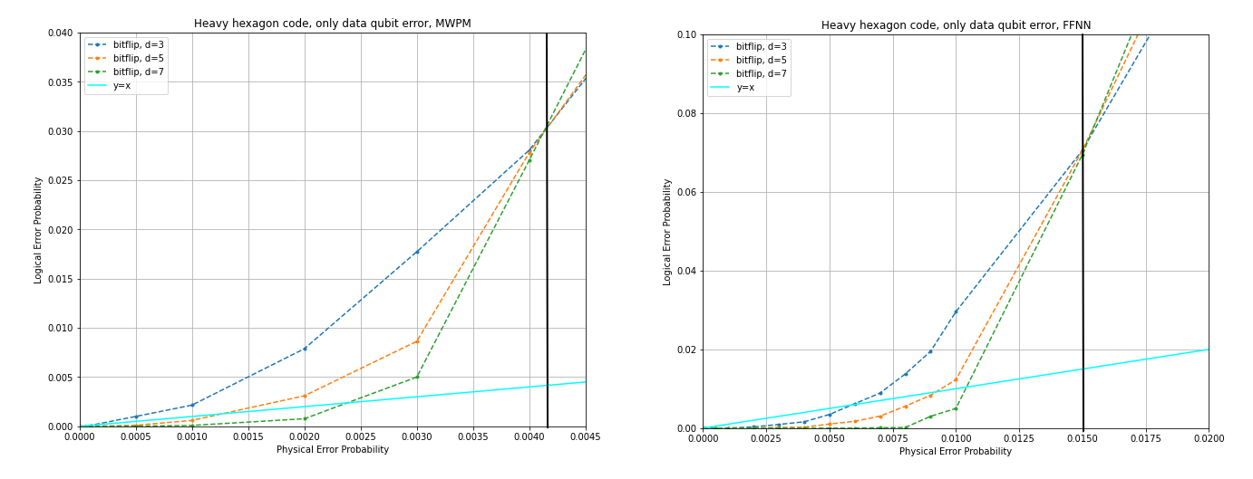
Figure 5. Threshold and pseudo-threshold values for MWPM and ML based decoders in case of distance 3, 5, and 7 heavy hexagonal code for bitflip error on data qubit

In Fig. 5, we show the increase in the logical error probability with physical error probability $p$, which is the probability of error per step in the heavy hexagonal code cycle. The results of MWPM and FFNN-based decoder for bitflip noise models on data qubits are shown. In Tables 3 we note the threshold value for both decoders and pseudo-threshold values for both decoders in case of distance 3, 5, and 7. In Fig. 5, the blue, orange, and green lines respectively are for distance 3, 5, and 7. The cyan straight line consists of the points where the probabilities of physical and logical error are equal.

The point where the decoder curves and the straight line intersects, defines the value of pseudo-threshold for the decoder. As expected, the pseudo threshold improves with increasing distance of the heavy hexagon code. Nevertheless, the threshold value is the probability of physical error beyond which increasing the distance leads to poorer performance. Therefore, threshold is independent of the distance and is a property of the error correcting code and the noise model only. Here we observe that ML- based decoders are working better than MWPM decoders in heavy hexagonal QECC in terms of threshold.

5.3.2. Comparison of FFNN based decoder result without and with gauge equivalence in case of bitflip error on data qubit along with measurement, and stabilizer error

Then we show the decoding performance of our FFNN-based decoder for heavy hexagon codes of distances 3, 5, and 7 for bitflip noise model on data qubit along with measurement, and stabilizer error for three cases, i.e. without gauge equivalence, with search-based gauge equivalence minimization, and with rank-based gauge equivalence minimization. Our FFNN based model outperforms the performance of the existing MWPM decoder. We also show that the performance of FFNN with gauge equivalence is better than FFNN without gauge equivalence, and also the performance of search based and rank based gauge equivalence is more or less equal. We then produce the comparison of decoding time (in seconds) needed for distance 5 and 7 heavy hexagon code in case of FFNN based decoder for 3 different case - without gauge equivalence, with search based gauge equivalence and with rank based gauge equivalence which supports the fact that rank based gauge equivalence method is faster than search based gauge equivalence minimization (Fig 7). Though the time needed for the basic FFNN decoder is much lesser than search based gauge or rank based gauge but the decoding performance is poorer as we have already stated.

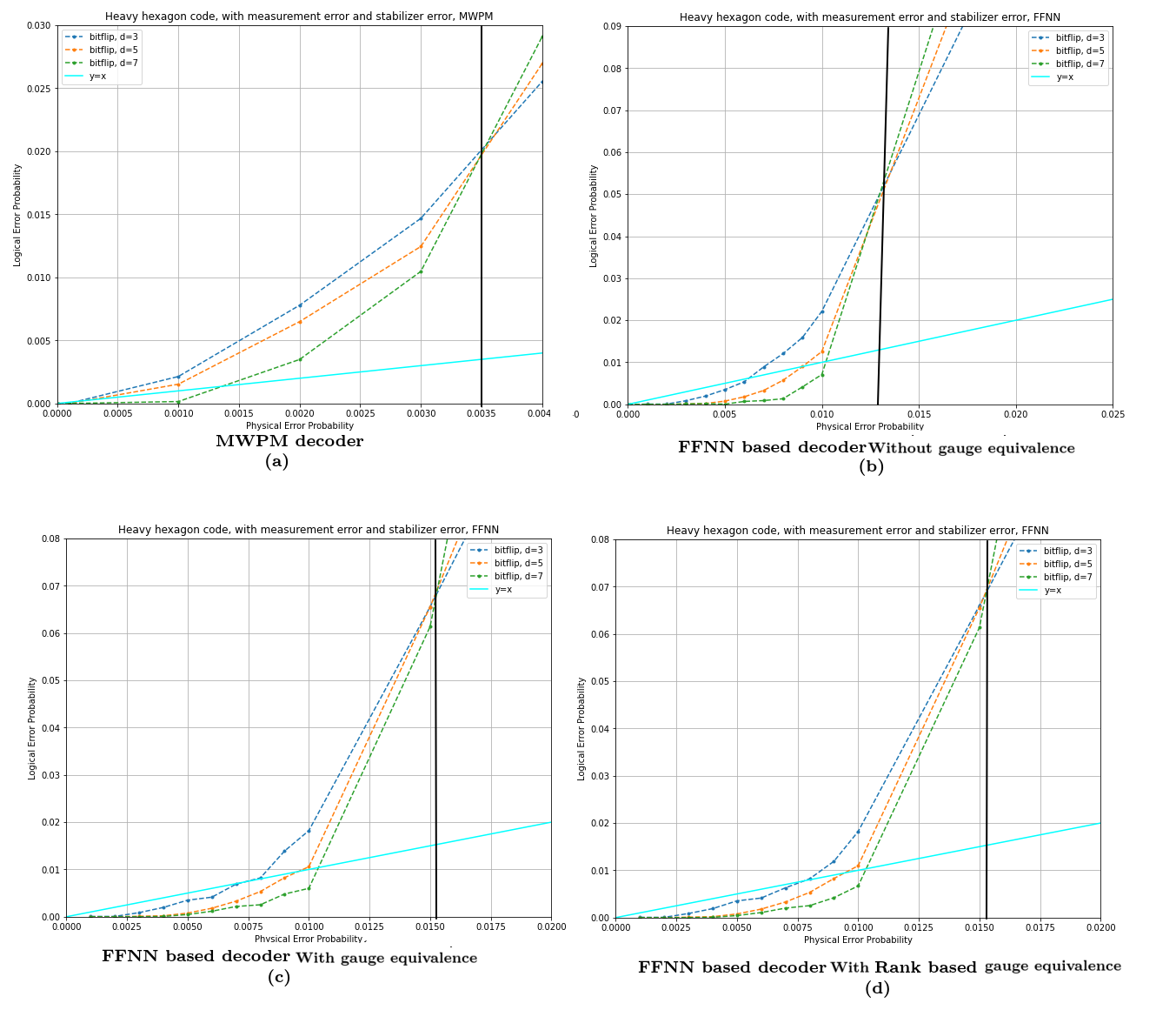
Figure 6. Threshold and pseudo-threshold values for MWPM and ML based decoders (without and with gauge equivalence) and in case of distance 3, 5, and 7 heavy hexagonal code for bitflip error on data qubit along with measurement, and stabilizer error

In Fig. 6, we show the increase in the logical error probability with physical error probability $p$, which is the probability of error per step in the heavy hexagonal code cycle.

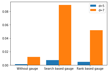
Figure 7. Comparison of decoding time (in seconds) needed for distance 5 and 7 heavy hexagon code in case of FFNN based decoder for 3 different case - without gauge equivalence (blue), with search based gauge equivalence (orange) and with rank based gauge equivalence (green)

	Threshold		Pseudo Threshold
		d=3	0.00018
MWPM	0.0035	d=5	0.00023
		d=7	0.0013
		d=3	0.0055
FFNN without gauge equivalence	0.01375	d=5	0.008
		d=7	0.011
		d=3	0.0081
FFNN with search based gauge equivalence	0.01586	d=5	0.0102
		d=7	0.0112
		d=3	0.0082
FFNN With rank based gauge equivalence	0.01587	d=5	0.0103
		d=7	0.0112

Table 4. Comparison of FFNN based decoder result without and with gauge equivalence in case of bitflip error on data qubit along with measurement, and stabilizer error

In Table 4 we note the threshold value for MWPM and FFNN based decoders (With and Without Using Gauge equivalence) and pseudo-threshold values for both decoders in case of distance 3, 5, and 7, for this same noise model. Here we observe $\sim 1.15\times$ (that is about $\sim 14\%$) increase in the threshold for ML-decoders using gauge equivalence as compared to ML-decoders without using gauge equivalence.

5.3.3. Depolarization noise model

Then we show the decoding performance of our FFNN-based decoder for heavy hexagon codes of distances 3, 5, and 7 for depolarizing noise models in terms of Logical $X$ (bitflip) and Logical $Z$ (phase flip) errors. Our model outperforms the performance of the existing decoders.

	Threshold		Pseudo-threshold
		d=3	0.0005
MWPM	0.0045	d=5	0.002
		d=7	0.0032
		d=3	0.0105
FFNN ( with gauge equivalence)	0.0245	d=5	0.0125
		d=7	0.0207

Table 5. Comparison of FFNN based decoder result with MWPM decoder for logical $X$ in depolarization noise model

Hence for depolarization noise model, using FFNN based decoder, the threshold is 0.0245 in case of heavy hexagon code. Note: For depolarization noise model, using FFNN based decoder, the threshold was 0.03 in case of surface code (bhoumik2022ml, ).

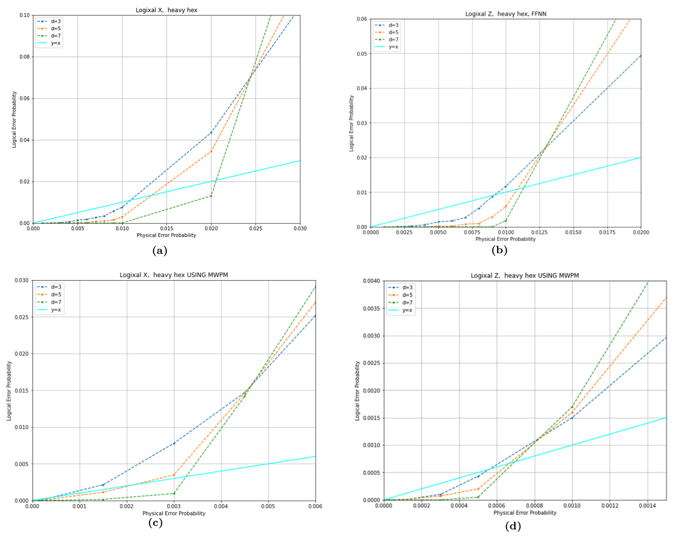
Figure 8. In FFNN based decoder (a) Logical $X$ error rates and (b) logical $Z$ error rates for the heavy hexagon code. In MWPM based decoder (a) Logical $X$ error rates and (b) logical $Z$ error rates for the heavy hexagon code.

6. Discussion

In this paper, we have proposed an ML-decoder for heavy hexagon code which makes use of a novel technique based on gauge equivalence to improve the performance of decoding. First we map decoding to a ML based classification problem. Exploiting the properties of heavy hexagon code as a subsystem code, we have defined gauge equivalence, which, in turn, reduces the number of error classes for ML based classification. We have proposed search based and rank based methods for finding the gauge equivalence; the former being faster for finding equivalence in phase flip errors and the later for bit flip errors.

We have empirically tested our decoders for distance 3, 5, and 7 heavy hexagon codes. We have shown that even the naive ML decoder outperforms the MWPM based decoder in terms of pseudo-thresholds and threshold. Moreover using gauge equivalence leads to further improvement in the decoder performance. This research provides a plausible method for scaling current quantum devices to the fault-tolerant era. Future directions may be to study the applicability of gauge equivalence and ML based decoders for other noise models such as Pauli and amplitude damping noise.

References

- [1] Peter W. Shor. Polynomial-time algorithms for prime factorization and discrete logarithms on a quantum computer. SIAM J. Comput., 26(5):1484–1509, October 1997.
- [2] Lov K. Grover. A fast quantum mechanical algorithm for database search. In Proceedings of the Twenty-eighth Annual ACM Symposium on Theory of Computing, STOC ’96, pages 212–219, New York, NY, USA, 1996. ACM.
- [3] Frank Arute, Kunal Arya, Ryan Babbush, Dave Bacon, Joseph C Bardin, Rami Barends, Rupak Biswas, Sergio Boixo, Fernando GSL Brandao, David A Buell, et al. Quantum supremacy using a programmable superconducting processor. Nature, 574(7779):505–510, 2019.
- [4] Ashley Montanaro. Quantum speedup of monte carlo methods. Proceedings of the Royal Society A: Mathematical, Physical and Engineering Sciences, 471(2181):20150301, 2015.
- [5] Peter W. Shor. Scheme for reducing decoherence in quantum computer memory. Phys. Rev. A, 52:R2493–R2496, Oct 1995.
- [6] A. M. Steane. Error correcting codes in quantum theory. Phys. Rev. Lett., 77:793–797, Jul 1996.
- [7] Raymond Laflamme, Cesar Miquel, Juan Pablo Paz, and Wojciech Hubert Zurek. Perfect quantum error correcting code. Phys. Rev. Lett., 77:198–201, Jul 1996.
- [8] Austin G Fowler, Adam C Whiteside, and Lloyd CL Hollenberg. Towards practical classical processing for the surface code. Physical review letters, 108(18):180501, 2012.
- [9] Debasmita Bhoumik, Pinaki Sen, Ritajit Majumdar, Susmita Sur-Kolay, Latesh Kumar KJ, and Sundaraja Sitharama Iyengar. Machine-learning based decoding of surface code syndromes in quantum error correction. Journal of Engineering Research and Sciences, 1(6):21–35, 2022.
- [10] Eric Dennis, Alexei Kitaev, Andrew Landahl, and John Preskill. Topological quantum memory. Journal of Mathematical Physics, 43(9):4452–4505, 2002.
- [11] Austin G Fowler, Ashley M Stephens, and Peter Groszkowski. High-threshold universal quantum computation on the surface code. Physical Review A, 80(5):052312, 2009.
- [12] David S Wang, Austin G Fowler, and Lloyd CL Hollenberg. Surface code quantum computing with error rates over 1%. Physical Review A, 83(2):020302, 2011.
- [13] James R Wootton and Daniel Loss. High threshold error correction for the surface code. Physical review letters, 109(16):160503, 2012.
- [14] Sergey B Bravyi and A Yu Kitaev. Quantum codes on a lattice with boundary. arXiv preprint quant-ph/9811052, 1998.
- [15] Christopher Chamberland, Guanyu Zhu, Theodore J Yoder, Jared B Hertzberg, and Andrew W Cross. Topological and subsystem codes on low-degree graphs with flag qubits. Physical Review X, 10(1):011022, 2020.
- [16] Dave Bacon. Operator quantum error-correcting subsystems for self-correcting quantum memories. Physical Review A, 73(1):012340, 2006.
- [17] Christopher Chamberland and Pooya Ronagh. Deep neural decoders for near term fault-tolerant experiments. arXiv preprint arXiv:1802.06441, 2018.
- [18] Jack Edmonds. Paths, trees, and flowers. Canadian Journal of Mathematics, 17:449–467, 1965.
- [19] Savvas Varsamopoulos, Ben Criger, and Koen Bertels. Decoding small surface codes with feedforward neural networks. Quantum Science and Technology, 3(1):015004, 2017.
- [20] Stefan Krastanov and Liang Jiang. Deep neural network probabilistic decoder for stabilizer codes. Scientific reports, 7(1):1–7, 2017.
- [21] R. Sweke et al. Reinforcement learning decoders for fault-tolerant quantum computation. arXiv preprint arXiv:1810.07207, 2018.
- [22] Savvas Varsamopoulos, Koen Bertels, and Carmen Garcia Almudever. Comparing neural network based decoders for the surface code. IEEE Transactions on Computers, 69(2):300–311, 2019.
- [23] P Baireuther et al. Machine-learning-assisted correction of correlated qubit errors in a topological code. Quantum, 2:48, 2018.
- [24] Gilbert Strang. Linear algebra and its applications. Belmont, CA: Thomson, Brooks/Cole, 2006.
- [25] Thomas H Cormen, Charles E Leiserson, Ronald L Rivest, and Clifford Stein. Introduction to algorithms. MIT press, 2022.
- [26] Michael A Nielsen and Isaac Chuang. Quantum computation and quantum information, 2002.