TFAD: A Decomposition Time Series Anomaly Detection Architecture with Time-Frequency Analysis

Abstract.

Time series anomaly detection is a challenging problem due to the complex temporal dependencies and the limited label data. Although some algorithms including both traditional and deep models have been proposed, most of them mainly focus on time-domain modeling, and do not fully utilize the information in the frequency domain of the time series data. In this paper, we propose a Time-Frequency analysis based time series Anomaly Detection model, or TFAD for short, to exploit both time and frequency domains for performance improvement. Besides, we incorporate time series decomposition and data augmentation mechanisms in the designed time-frequency architecture to further boost the abilities of performance and interpretability. Empirical studies on widely used benchmark datasets show that our approach obtains state-of-the-art performance in univariate and multivariate time series anomaly detection tasks. Code is provided at https://github.com/DAMO-DI-ML/CIKM22-TFAD.

1. Introduction

With the rapid development of the Internet of Things (IoT) and other monitoring systems, there has been an enormous increase in time series data (Wen et al., 2022; Faloutsos et al., 2020). Thus, effectively monitoring and detecting anomalies or outliers on the time series data is crucial to discovering faults and avoiding potential risks in many real-world applications. Generally, an anomaly is an observation that deviates from normality. Anomaly detection has been studied widely in different disciplines, including statistics, data mining, and machine learning (Ruff et al., 2021), but how to perform it effectively on time series data is an active research topic and has received a lot of attentions recently (Ren et al., 2019; Gao et al., 2020; Zhang et al., 2021; Lai et al., 2021; Tuli et al., 2022; Li et al., 2022; Patel et al., 2022) due to the special properties of time series.

Unlike ordinary tabular data, one distinguishing property of time series is the temporal dependencies. Usually, a point or a subsequence of time series is called an anomaly when compared to its corresponding “context”. Based on the relationship between the anomaly in time series and its context, we can define different types of anomalies, such as global point anomaly, seasonality anomaly, shapelet anomaly, etc. Thus, the first challenge in time series anomaly is how to model the relationship between a point/subsequence and its temporal context for different types of anomalies. Secondly, like other anomaly detection tasks, anomaly happens rarely, and there is usually limited labeled data for data-driven models. A possible solution is data augmentation, which is widely used in deep learning training (Shorten and Khoshgoftaar, 2019). Although some data augmentation methods have been proposed for time series data (Wen et al., 2021b), how to design and apply data augmentation in time series anomaly detection remains an open problem.

As a typical signal, the time series data can be analyzed not only from the time domain but also from the frequency domain (Hamilton, 1994). Most of the existing methods, including conventional and deep methods, focus mainly on time-domain modeling and do not fully utilize the information in the frequency domain. The frequency domain can provide vital information for time series, such as seasonality (Wen et al., 2021a). In addition, it is much easier to detect in the frequency domain than in the time domain for some complex group anomalies and seasonality anomalies. Recently, there have been some attempts to model time series from the frequency domain (Parhizkar et al., 2015), such as the data augmentation in the frequency domain (Gao et al., 2020). Unfortunately, how to systematically and directly utilize the frequency domain and time domain information simultaneously in modeling time series anomaly detection is still not fully explored in the literature.

In this paper, to better detect various kinds of time series anomalies, we proposed a Time-Frequency domain analysis time series Anomaly Detection model, TFAD. It mainly contains two branches: the time-domain analysis branch and the frequency domain analysis branch. Specifically, with a well-designed window-based model structure, we implement a time series decomposition module to detect anomalies in different components with interference among different components reduced and a representation learning module with a neural network to gain richer sequence information. To deal with the challenges of insufficient anomaly data, we conduct data augmentation of TFAD in different views: normal data augmentation, abnormal data augmentation (not fully considered in existing works), time-domain data augmentation, and frequency domain data augmentation.

In summary, our main contributions are listed as follows:

• We integrate the frequency domain analysis branch with the time domain analysis branch to identify the temporal information and improve detection performance.

• We combine the time series decomposition module with a concise neural representation network. With the help of time series decomposition, a simple temporal convolution neural network performs well. Moreover, it makes the model easy to be implemented, and the anomaly results of different components give insights into why it is abnormal.

• Various data augmentation methods, besides normal data augmentation and time domain data augmentation, abnormal data augmentation and frequency domain data augmentation are also implemented to overcome the lack of anomaly data.

The rest of the paper is organized as follows. In Section 2, we review the related work. In Section 3, we briefly introduce the definitions of time series anomalies. In Section 4, we introduce our proposed TFAD algorithm, including motivations, architecture, and network design. In Section 5, we evaluate our algorithm empirically on both univariate and multivariate time series datasets in comparison with other state-of-the-art algorithms. An ablation study is also performed to analyze different modules in the network. And we conclude our discussion in Section 6.

2. Related Work

Both traditional and deep methods have been applied in time series anomaly detection tasks. A survey of traditional techniques for time series anomaly detection is in (Gupta et al., 2013). Traditional techniques can be roughly classified as similarity-based (Lane et al., 1997; Guan et al., 2016), window-based (Gao et al., 2002), decomposition-based (Gao et al., 2020; Wen et al., 2019), deviants detection based methods (Muthukrishnan et al., 2004), et al. With the rapid development of deep learning, a vast of deep anomaly detection methods emerge (Kiran et al., 2018; Hendrycks et al., 2018; Ruff et al., 2021), including one-class type SVDD-based model (Ruff et al., 2018), reconstruction type GAN/VAE-based model (Rezende et al., 2014), et al. Deep methods are also applied in time series anomaly detection (Shen et al., 2020; Xu et al., 2022; Zong et al., 2018).

According to the input data type, there are methods designed for univariate time series, multivariate time series, or both. According to the access of labels, there are unsupervised, semi-supervised, and supervised time series anomaly detection methods. Online anomaly detection (Chen et al., 2022a; Bock et al., 2022) is also quite different from offline settings. For univariate time series anomaly detection, many traditional methods have been designed (Ren et al., 2019; Siffer et al., 2017; Xu et al., 2018). POT (Siffer et al., 2017) proposes an approach based on Extreme Value Theory to detect outliers without the assumption of distribution. M-ELBO (Xu et al., 2018) designs a VAE-based algorithm on the Yahoo dataset. For multivariate time series anomaly detection, the development of representation learning stimulates blowout growth in the multivariate time series anomaly detection field. THOC (Shen et al., 2020) proposes a temporal classification model for time series anomaly detection by capturing temporal dynamics in multi scales. It follows the one-class classification framework generally used (Ruff et al., 2021, 2018). Anomaly Transformer (Xu et al., 2022) designs unsupervised anomaly detection methods combining the transformer framework with a point-wise prior association by a mini-max strategy. Generative models, such as DAGMM (Zong et al., 2018), AnoGAN(Schlegl et al., 2017), and LSTM-VAE (Park et al., 2018), also form a mainstream research direction. Some surveys compare different kinds of anomaly detection methods in time series (Freeman et al., 2021; Blázquez-García et al., 2021).

The most related work of this paper is (Carmona et al., 2022), which introduces a window-based framework for anomaly detection in time series applied in unsupervised/supervised and univariate/multivariate settings. However, like most existing anomaly detection methods, it only works in the time domain. Although it works well for point-wise anomalies, it is usually hard to detect complex pattern anomalies, e.g., a sub-sequence time series. Instead, AutoAI-TS (Shah et al., 2021) also takes the advantage of frequency domain analysis for period/seasonal forecasting. In summary, our designed TFAD model contains two branches: the time-domain analysis branch and the frequency domain analysis branch, which is different from existing works. Besides, the time series decomposition module used in traditional methods is also implemented in our TFAD architecture. Furthermore, several well-designed data augmentation methods are also considered in TFAD to gain rich, reasonable, and reliable dataset.

3. Preliminaries

In this Section, we will first give a brief view of the definitions of general anomalies. Anomalies appear in many situations. Anomalies in time series are a special type as the point without information of neighbor points means nothing. Such characteristics make time series analysis different from others. Thus, we will also show the definitions of time series or more specially, saying, sequential anomaly definitions.

3.1. General Anomaly Definitions

In applications with non-sequential data, set $\mathcal{D}\in R$ as the data space and the normality follows distribution $\mathcal{N}^{+}$. Assuming $\mathcal{N}^{+}$ has a corresponding probability density function $p^{+}$, then the anomalies can be set as

(1) $$A=\{d\in\mathcal{D}\ |p^{+}(d)\leq\tau\},\tau>0,$$

where $\tau$ is the threshold of anomaly.

Anomalies in non-sequential data can be mainly classified into three types: point anomaly, contextual anomaly, and group anomaly. A point anomaly is an individual data point that deviates from normality and is the most common case in anomaly detection. It can also be called a global anomaly. A context anomaly is also called a conditional anomaly. It is anomalous in a specific context. For instance, the temperature of 20 degrees is normal in most areas but abnormal in Antarctica. A group or collective anomaly is a group of points that abnormal.

3.2. Sequential Anomaly Definitions

Time series data is a sequence of data points $X=(x_{0},x_{1},x_{2},\cdots,x_{n})$ where $x_{i}$ is the point at timestamp $i$. More specially, time series can be formally defined by structural modeling (Shumway et al., 2000; Lai et al., 2021) to include trend, seasonality and shapelets, as

(2) $$X=\sum_{n}\{A\sin(2\pi\omega_{n}T)+B\cos(2\pi\omega_{n}T)\}+\tau(T),$$

where $T=(1,2,3,\cdots,n)$ is a series of timestamps, $\omega_{n}$ is the frequency of wave $n$, $A,B$ are coefficients, the combination of sinusoidal wave represents the shapelets and seasonality, and $\tau(T)$ is trend component.

The definitions in a non-sequential context can not sufficiently define the group and context anomalies in sequential data. Instead, sequential anomalies can be classified as point anomaly (global point anomaly and context point anomaly) and pattern anomaly (shapelet anomaly, seasonal anomaly, and trend anomaly) (Lai et al., 2021), as shown in Figure 1.

Formally, point-wise anomalies can be defined as ${|x_{t}-\hat{x_{t}}|}>{\sigma}$ where $\hat{x_{t}}$ is the expected value and $\sigma$ is threshold. Shapelet anomaly can be defined as $s(\rho(\cdot),\hat{\rho}(\cdot))>\sigma,$ where function $s$ measures the difference between two subsequences, $\hat{\rho}$ is the expected shapelet and $\sigma$ is a threshold. Seasonal anomaly refers to subsequence with abnormal seasonality and it is defined as $s(\omega,\hat{\omega})>\sigma$ where $\hat{\omega}$ is expected seasonality. Trend anomaly is a subsequence whose trend alters the trend of $X$. It can be defined as $s(\tau(\cdot),\hat{\tau}(\cdot))>\sigma$ where $\hat{\tau}$ is the expected trend of subsequence.

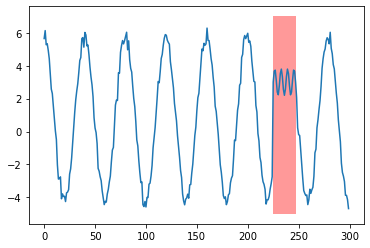
(a) shapelet anomaly

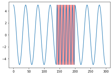
(b) seasonal anomaly

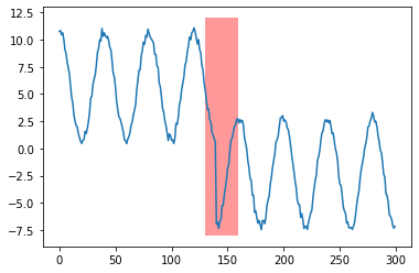
(c) trend anomaly

(d) global point anomaly

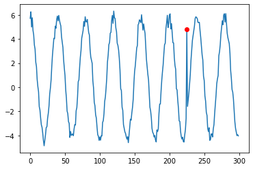
(e) context point anomaly

Figure 1. Anomalies in time series.

4. Proposed TFAD Algorithm

4.1. Motivation: Time-Frequency Analysis

In this part, we will provide the design motivation of TFAD algorithm through the uncertainty principle of time-frequency analysis and demonstrate its effectiveness in time series anomaly detection.

4.1.1. Uncertainty Principle for Time Series Representation in Time and Frequency Domains

The uncertainty principle expresses a fundamental relationship between the standard deviation of a continuous function and the standard deviation of its Fourier transformation (Cohen, 1995). Let the input signal $s(t)$ have a spectrum $S(\omega)$ as

(3) $$S(\omega)=\frac{1}{\sqrt{2\pi}}\int_{-\infty}^{\infty}s(t)e^{-j\omega t}dt.$$

The standard deviations of the time and frequency density functions, $\sigma_{t}$ and $\sigma_{\omega}$, are defined as the parameters that describe the broadness of the signal in time and frequency domains, respectively

(4) $$\sigma_{t}^{2}=\int(t-<t>)^{2}|s(t)|^{2}dt,~{}~{}\sigma_{\omega}^{2}=\int(\omega-<\omega>)^{2}|S(\omega)|^{2}d\omega.$$

Then we have the following result based on Schwarz inequality

(5) $$\sigma_{t}^{2}\sigma_{\omega}^{2} =\int|ts(t)|^{2}dt\times\int\left|s^{\prime}(t)\right|^{2}dt$$

$$\geq\left|\int ts^{\star}(t)s^{\prime}(t)dt\right|^{2}=\left|-\frac{1}{2}+j\operatorname{Cov}_{t\omega}\right|^{2}=\frac{1}{4}+\operatorname{Cov}_{t\omega}^{2}.$$

When we view the uncertainty principle from time series anomaly detection, it means that when one structure has a good catch of point-wise anomaly in the time domain, it would have a less sensitive detection power in the frequency domain, and vice versa. Designing a model with a single structure that can detect the time and frequency simultaneously is difficult. A better approach could be using different structures to detect them and merge them as a whole model.

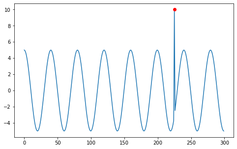
(a) Point-wise anomaly example

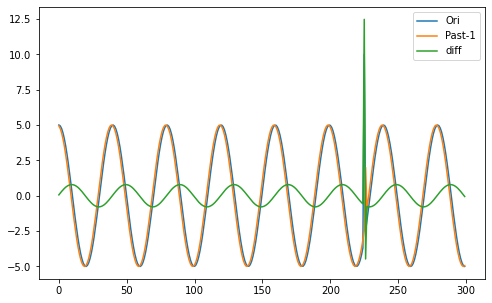
(b) Diff in time domain w/o point-wise anomaly

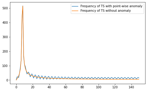
(c) Diff in frequency domain w/o point-wise anomaly

Figure 2. Examples of point-wise anomaly in time and frequency domain.

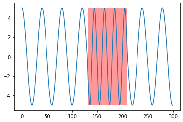
(a) Seasonality anomaly example.

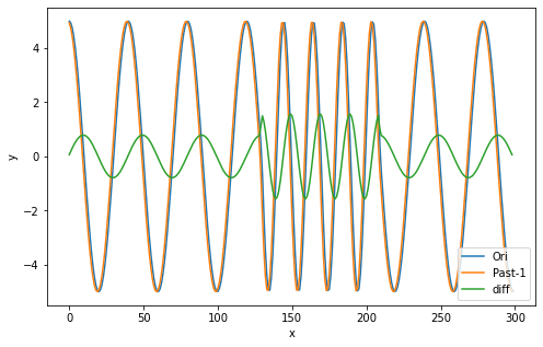
(b) Diff in time domain w/o seasonality anomaly

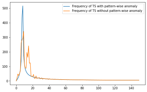
(c) Diff in frequency domain w/o seasonality anomaly

Figure 3. Examples of pattern-wise anomaly in time and frequency domain.

4.1.2. Understanding the Limitations of Single Domain Analysis

This subsection will show the significant difference in point-wise anomaly detection and pattern-wise anomaly detection intuitively by two simple examples and demonstrate the limitations of detecting anomalies only in the time or frequency domain. The illustration examples are plotted in Figure 2 and Figure 3, where Figure 2 shows the differences between the detection of point-wise anomaly in time domain (fig 2(b)) and frequency domain (fig 2(c)) by a global point anomaly example (fig 2(a)), and Figure 3 shows the differences between the detection of pattern wise anomaly in time domain (fig 3(b)) and frequency domain (fig 3(c)) by a seasonality anomaly example (fig 3(a)).

Generally, anomaly detection in time domain is done by comparing the point with its past neighbors. For simplicity, assume the time step is one between two adjacent points. We show the analysis in time domain intuitively by computing the difference (noted as diff) between the original point (noted as Ori) and the point before it (noted as Past-1). Figure 2(b) and figure 3(b) show the different results in time domain of the point-wise anomaly example and pattern-wise anomaly example, respectively. It can be seen that point anomaly is easier to be detected than seasonality anomaly in time domain analysis. Detecting seasonality anomalies only through time-domain analysis is not easy.

For anomaly detection in the frequency domain, we compare the time series results with/without anomalies after time to frequency transform (by Fourier transform). Figure 2(c) shows results of the time series in frequency domain with and without point-wise anomalies. The difference is subtle and disperses in many channels, indicating it is hard to detect point-wise anomaly only with time domain analysis. Figure 3(c) shows the results of time series in frequency domain with and without seasonality-wise anomaly. Unlike the situation in point-wise anomalies, the difference is quite evident as different numbers of peaks are shown. Thus, seasonality anomaly is easier to detect than point anomaly in frequency domain analysis. It is impractical to detect point-wise anomalies only by frequency domain analysis.

4.2. Motivation: Data Augmentation and Decomposition

Besides the time-frequency analysis, we also consider data augmentation and decomposition to further improve the performance of time series anomaly detection.

4.2.1. Time Series Data Augmentation

The performance of machine learning usually relies on many training data. However, in reality, labeled data is usually limited. Data augmentation (Wen et al., 2021b) contributes a lot to help mitigate these challenges. Unlike most existing works where augmented data should follow the original data distribution, we consider two kinds of data augmentation methods for the anomaly detection task: Data augmentation for normal data and anomaly data. In the anomaly detection task, anomalies are samples different from normal data. There are usually various kinds of anomalies. Thus, when anomaly data is augmented, there is no need to create anomalies identical to real anomalies in the dataset, which is also impractical. Diverse augmented anomalies generally contribute to the robustness of models.

4.2.2. Time Series Decomposition

Generally speaking, time-series data often exhibit various patterns, and it is usually helpful to split a time series into main components. It is a powerful technology for analyzing complex time series widely adopted in time series anomaly detection (Hochenbaum et al., 2017; Gao et al., 2020; Zhang et al., 2021) and forecasting (Zhou et al., 2022; Xu et al., 2021; Chen et al., 2022b). Furthermore, with the help of time series decomposition, simple temporal convolution neural networks can bring desirable performance (this will be discussed later). It makes the model easy to be implemented and provides insights based on anomaly results of different components.

4.3. High Level Architecture of TFAD

Following the aforementioned motivations, the high level architecture of our designed TFAD algorithm is summarized in Fig 4. Our method consists of two main branches, the time-domain analysis branch and the frequency-domain analysis branch. Besides that, both normal data augmentation module and anomaly data augmentation module are designed to increase the robustness of our method. Furthermore, the time series decomposition module is adopted to better detect anomalies in different components and provide insights into the explanation of anomalies.

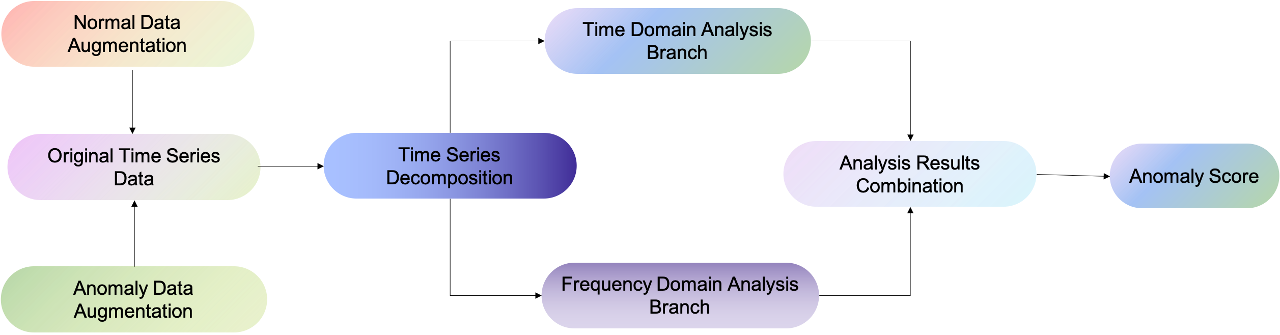
Figure 4. High-level diagram of TFAD architecture.

4.4. Network Design of TFAD

In this section, we provide the detailed design of the TFAD algorithm. The whole network structure of TFAD is plotted in Fig. 5, where each module will be elaborated in the following parts.

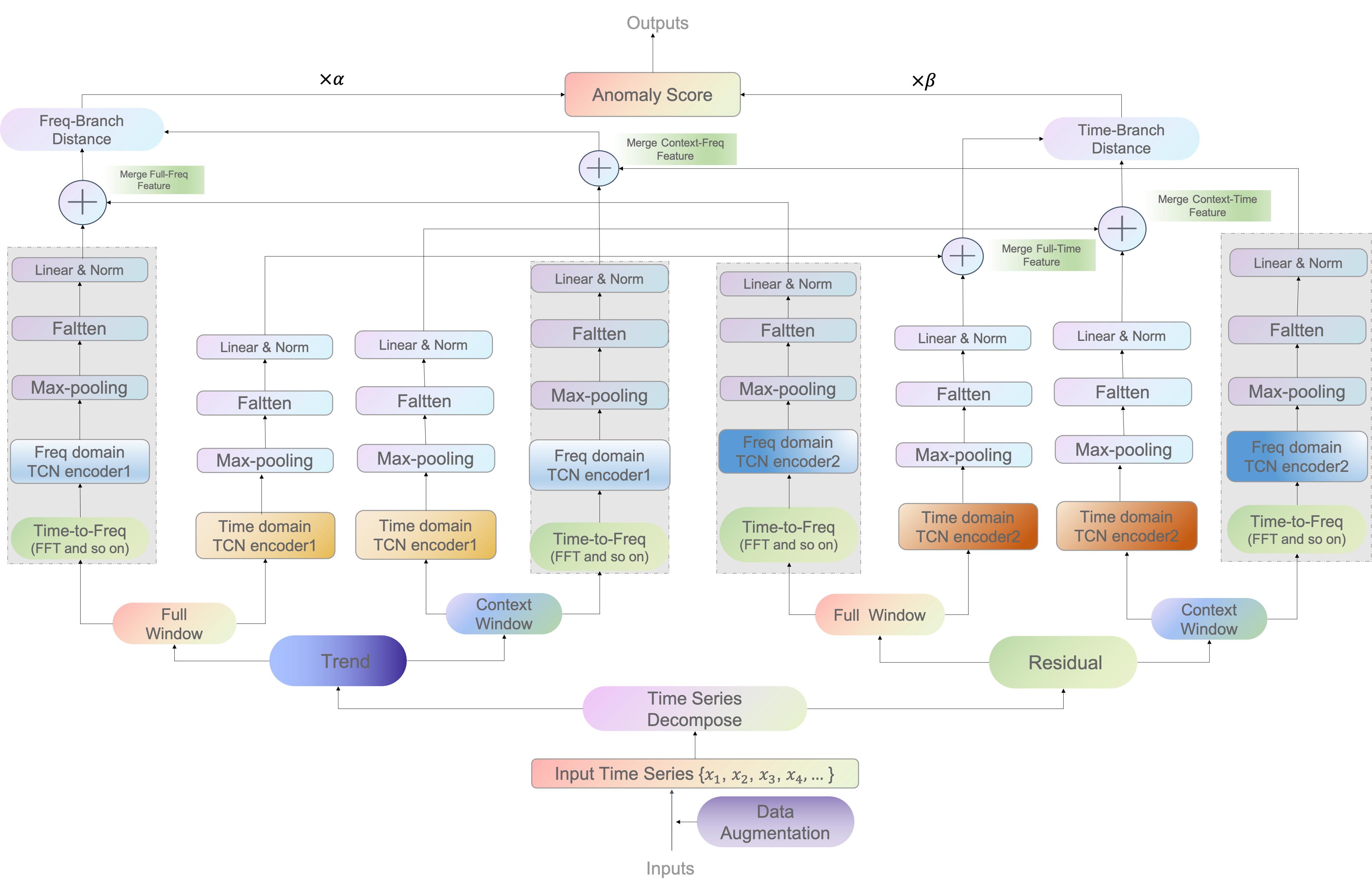
Figure 5. Network structure of the proposed TFAD algorithm. The shaded blocks indicate the frequency domain branch.

4.4.1. Data Augmentation Module

As discussed before, we consider both normal and anomaly data augmentation.

For normal data augmentation, firstly, we generate data with low noise, which is more normal. Robust STL (Wen et al., 2019) is a desirable option to get trend and seasonal information of time series data, and the residual, which is in some way noise, can be ignored. Such more normal data keep the innate character of normal patterns and have larger differences with anomalies. It is easier to distinguish more normal data from anomalies and helps our model learn the intrinsic quality of normal data. To create diverse normal data, we transfer time series to the frequency domain by Fourier transform and make small changes in both the imaginary and the real parts to gain new data. In this way, diverse data is augmented. An example is shown in Figure 6.

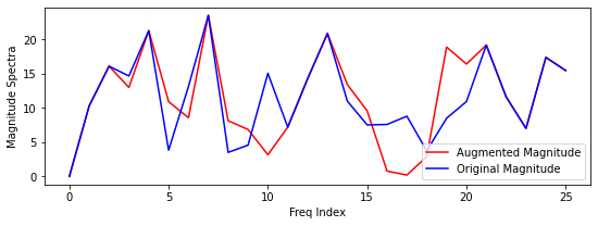
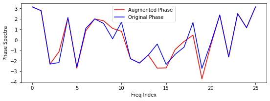
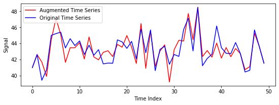
Figure 6. Norm data augmentation by frequency domain changes.

Besides the typical anomalies in the data set for anomaly data augmentation, other possible anomalies should also be considered for anomaly data augmentation. It helps to detect new anomalies and contributes to the robustness of our method. Similar results also appear in the computer vision field (Ruff et al., 2020), which demonstrates that relatively few random outlier exposure images help to yield state-of-the-art detection performance. Specifically, we consider several data augmentation methods. Point scale modification in the time domain is adopted for point change anomaly, which is the most common type. For context anomalies, point/short sequence exchange and a mix-up between two different time series are considered. For anomalies in seasonal and some other complicated anomalies, several different data augmentation methods in the frequency domain are used to generate various sequence anomalies.

4.4.2. Decomposition Module

There are different kinds of methods to make time-series decomposition, for example, moving averages, classical decomposition methods such as additive decomposition and multiplicative decomposition, X11 decomposition method (Dagum and Bianconcini, 2016), seat decomposition method (Dagum and Bianconcini, 2016), and STL decomposition method (Robert et al., 1990). In this paper, Hodrick–Prescott (HP) filter (Hodrick and Prescott, 1997) is adopted for time series decomposition since it is easy to implement and works well in the real world.

Denote time series $y_{t}$, $t=\{1,2,\dots,T\}$ contains a trend component ${\tau}_{t}$, a residual part ${\epsilon}_{t}$. That is, $y_{t}=\tau_{t}+\epsilon_{t}$. Then, in HP filter, the trend component can be obtained by solving the following minimization problem

(6) $${\min}_{\tau}\left(\sum_{t=1}^{T}(y_{t}-\tau_{t})^{2}+\lambda\sum_{t=2}^{T-1}{[(\tau_{t+1}-\tau_{t})-(\tau_{t}-\tau_{t-1})]}^{2}\right),$$

where the multiplier $\lambda$ is the parameter that adjusts the sensitivity of the trend to fluctuation and can be adjusted according to the frequency of observations (Ravn and Uhlig, 2002). After decomposition, both trend and residual components are utilized to improve performance since different anomalies may appear in different components.

We mainly consider the decomposition method for univariate time series in TFAD. For multivariate time series, we decompose each time series sequence separately. It may not be the best method for multivariate time series decomposition. However, significant improvement is gained, and we will leave a special design for multivariate time series as future work.

4.4.3. Window Splitting Module

In the time series anomaly detection task, temporal correlations among observations are significant, and sequence anomalies are usually harder to be detected than point anomalies. Furthermore, even point anomaly is hard to be detected without temporal correlations. Therefore, we adopt time series window to better gain sequence-wise/temporal correlation information (Carmona et al., 2022; Tuli et al., 2022). Specifically, a full time series window and a context time series window are set to detect anomalies in a suspect sequence, where the full window consists of a context window and a suspect window, as illustrated in Figure 7. The assumption is that suppose the context window is normal. If the pattern of the full window is consistent with the pattern of the context window, then there is no anomaly in the suspect window. If there is an anomaly in the suspect window, the pattern of the full window will not be consistent with the context window. With sliding windows, the label of each time point can be known and more details are in Section 4.4.5.

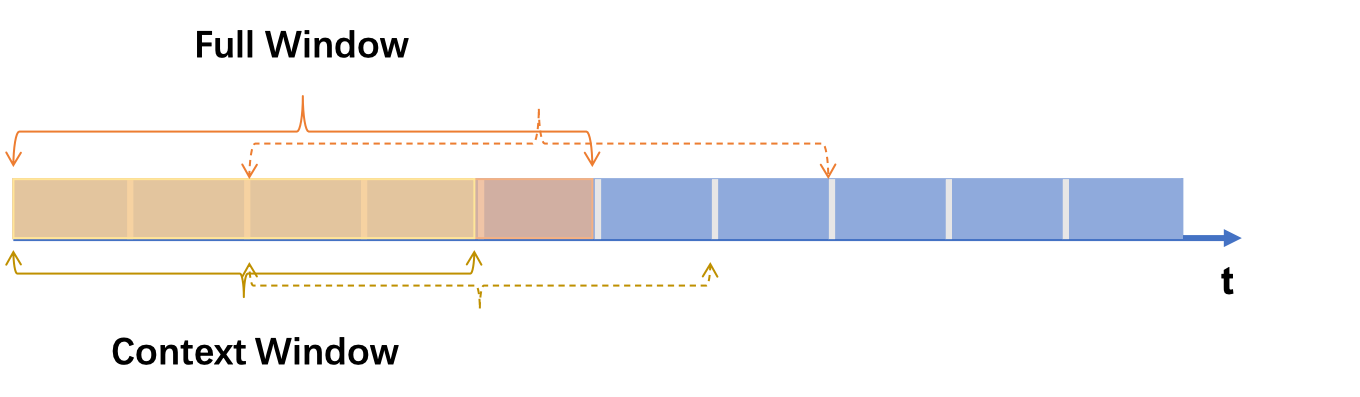
Figure 7. Window splitting.

4.4.4. Time and Frequency Branches

In this section, the time and frequency branches will be discussed. As shown in Fig 5, the original time series will be first decomposed into trend and residual components. For each component, we set the full window sequence and context window sequence with the aforementioned window splitting. After that, time-domain representation learning and frequency-domain representation learning for each window sequence will be done to gain rich information on sequences. After that, the distance between the context window and the full window would be measured to calculate the anomaly score.

For the representation, most of the classical distances, such as Cosine distance, dynamic time warping (DTW) distance, are too susceptible to the length of time series to be used here. Instead, neural networks are widely used to gain the representation of complex samples in many tasks due to the power of representation ability. Thus, we utilize a neural representation network to overcome the above shortcoming of classical methods. Specifically, the temporal convolutional network (TCN) (Bai et al., 2018) is a simple and powerful architecture. Therefore, we adopt the TCN design as our representation network.

TFAD first transforms the time series from time-domain to frequency-domain for the frequency branch by discrete Fourier transform (DFT). For time series $\{x_{n}\}:=x_{0},x_{1},\dots,x_{N-1}$, its discrete Fourier transform $\{X_{k}\}:=X_{0},X_{1},\dots,X_{N-1}$ is defined as

(7) $$X_{k}=\sum_{n=0}^{N-1}x_{n}\cdot e^{-\frac{i2\pi}{N}kn}\\ =\sum_{n=0}^{N-1}x_{n}\cdot\left[cos(\frac{2\pi}{N}kn)-i\cdot sin(\frac{2\pi}{N}kn)\right].$$

The results of DFT contain real-part (denoted as $Re$) and imaginary-part (denoted as $Im$). To better get the information of time series in different locations, TFAD intersects $Re$ and $Im$ and gets $\{X_{k}\}=F_{\{x_{n}\}}=\{Re_{1},Im_{1},Re_{2},Im_{2},\dots,Re_{n},Im_{n}\}$. After obtaining DFT results, representation learning is done by TCN similarly to the time branch.

There are different transform methods for time-frequency translation besides DFT, such as continuous Fourier Transform (CFT), short-time Fourier Transform (STFT), and wavelet transform. DFT is more suitable for our situation: the time-series data is usually discrete. As the length of the anomaly sequence is unknown, the window length of STFT is hard to set. Wavelet transform is considered to contain time and frequency information simultaneously, but evaluation shows that it does not gain a good performance as DFT. The main reason may be that, with the time-domain branch added already, a DFT with frequency information can gain more marginal utility than a wavelet.

4.4.5. Anomaly Score Module

Comparison between full window sequence and context window sequence is used to set anomaly score, which is a widely used metric for the degree of anomalousness (Ruff et al., 2021). Here, the cosine similarity between full window sequence and context window sequence is set as anomaly score. Specifically, denote anomaly score as $AS$, then

(8) $$AS=\mathcal{F}\{dis(RV_{treT},RV_{resT},RV_{treF},RV_{resF})\},$$

where $RV_{treT}$, $RV_{resT}$ are representation results of trend component and residual component in time domain respectively, $RV_{treF},RV_{resF}$ are representation results of trend component and residual component in frequency domain respectively, and the distance function $dis()$ is the cosine similarity. The higher the anomaly score is, the higher the dissimilarity is, which means the suspect window is more likely to be abnormal. We can decide whether the suspect window is abnormal with a threshold for anomaly score. Thus, suspect windows can be labeled with an anomaly or not. However, we also want to know what label should be set for every time point. Therefore, a voting strategy is adopted. With sliding full and context windows, the suspect window is also sliding. Every point belongs to several suspect windows, and if more than half of them are labeled as an anomaly, the point will be set as an anomaly.

5. Experiments

This section studies the proposed TFAD model empirically compared to other state-of-the-art time series anomaly detection algorithms on both univariate and multivariate time series benchmark datasets. We also investigate how each component in TFAD contributes to the final accurate detection by ablated studies and discuss the insights.

5.1. Baselines, Datasets, Metrics, and Evaluation

5.1.1. Baselines.

For univariate time series anomaly detection, we compare our method with the state-of-the-art algorithms, including SPOT, DSPOT (Siffer et al., 2017), DONUT (Xu et al., 2018), SR, SR-DNN, SR-CNN (Ren et al., 2019), and NCAD (Carmona et al., 2022). For multivariate time series anomaly detection, we compare recent deep neural network models like AnoGAN (Schlegl et al., 2017), DeepSVDD (Ruff et al., 2018), DAGMM (Zong et al., 2018), LSTM-VAE (Park et al., 2018), MSCRED (Zhang et al., 2019), OmniAnomaly (Su et al., 2019), MTAD-GAT (Zhao et al., 2020), THOC (Shen et al., 2020). Note that some baselines above are not designed for temporal data, but they are extended for time series data with fixed lengths by sliding windows.

5.1.2. Datasets.

We adopt the widely-adopted univariate and multivariate datasets for time series anomaly detection as follows:

• KPI (Competition, 2018) is a univariate time series dataset released in the AIOPS anomaly detection competition. It contains dozens of KPI curves with labeled anomaly points. The points are collected every 1 minute or 5 minutes from Internet Companies, for instance, Sogou, Tencent, eBay, etc.

• Yahoo (Research, 2015) is a univariate time series dataset for time series anomaly detection released by Yahoo research. Part of the dataset is synthetic, where the anomalies are algorithmically generated. Part of it is real traffic data to Yahoo services, where the anomalies are labeled manually by editors.

• SMAP and MSL (Hundman et al., 2018) are two multivariate time series datasets published by NASA. SMAP and MSL have 55 and 27 unique telemetry channels, respectively, that is, 55 and 27 dimensions time series. More specifically, anomaly sequences in SMAP are composed of $62\%$ point anomalies and $38\%$ contextual anomalies, while MSL consists of $53\%$ point anomalies and $47\%$ contextual anomalies.

The summary of these datasets is shown in Table 1.

Table 1. Summary of adopted datasets.

data set	$\#$Curves/Dims	$\#$Points	$\%$Anomaly
KPI	58	5922913	2.26
Yahoo	367	572966	0.68
SMAP	55	429735	12.8
MSL	27	66709	10.5

5.1.3. Metrics.

Point adjusted F1 score (Shen et al., 2020; Audibert et al., 2020; Su et al., 2019) is the widely used metric in the time series anomaly detection task. In this metric, if one point is detected as an anomaly in a segment, the whole anomaly segment will be considered as detected. This metric fits well with real-world situations as, in most cases, the anomaly event affects more than one time point. For such an abnormal event, a single anomaly alarm is enough. Note that several other F1-type metrics (Kim et al., 2022; Garg et al., 2021; Jacob et al., 2020; Hwang et al., 2022) have been proposed to provide a more precise evaluation of abnormal event detection. Either the first alarm of group anomalies is set with higher importance, or the proportion of alarms is evaluated. However, in this paper, our primary aim is not to discuss which metric is the best as different metrics are applied in different situations. Thus, we adopt the widely used point-adjusted F1 score as our metric and leave evaluations on more different metrics for future work.

5.1.4. Evaluation Details.

We follow the common setting as in (Ren et al., 2019; Carmona et al., 2022) for better comparisons. Specifically, we split each dataset into the train part, validation part, and test part to choose models. For the Yahoo dataset, we split 50% as test data, 30% as train data, and 20% as validation data. The original KPI dataset contains train and test data, and we set 30% of the training data as validation data. For the evaluation of the KPI dataset, we apply both supervised setting (sup.) where all labeled data are utilized and unsupervised setting (un.) where the label information is not utilized. Every setting has been run ten times, and the mean and variance are reported.

5.2. Performance Comparisons

The performance comparisons of different baseline algorithms and our TFAD are summarized in Table 2 and Table 3 for univariate and multivariate time series anomaly detection tasks, respectively.

For the univariate time series anomaly detection in Table 2, it can be seen that deep learning methods usually bring better performance than the conventional methods like SPOT and DSPOT, due to their strong representation abilities. Note that both NCAD (Carmona et al., 2022) and our TFAD introduce data augmentation, and the randomness of augmented data brings in fluctuation in the F1 score. The variance of TFAD is significantly lower than NCAD in most cases, which indicates our TFAD method would be more robust and stable in practical systems. In summary, our TFAD algorithm produces comparable performance to the best NCAD algorithm on the Yahoo dataset, and significantly outperforms all other competing algorithms on the KPI dataset.

Table 2. F1 score of anomaly detection on univariate time series datasets. The best results are highlighted.

Model	Yahoo (un.)	KPI (un.)	KPI (sup.)
SPOT	33.8	21.7	–
DSPOT	31.6	52.1	–
DONUT	2.6	34.7	–
SR	56.3	62.2	–
SR-CNN	65.2	77.1	–
SR-DNN	–	–	81.1
NCAD	$\textbf{81.16}\pm 1.43$	$76.64\pm 0.89$	$79.20\pm 0.92$
TFAD	${81.13}\pm\textbf{0.52}$	$\textbf{79.80}\pm\textbf{0.74}$	$\textbf{82.10}\pm\textbf{0.42}$

Table 3. F1 score of anomaly detection on multivariate time series datasets. The best results are highlighted.

Model	SMAP (un.)	MSL (un.)
AnoGAN	74.59	86.39
DeepSVDD	71.71	88.12
DAGMM	82.04	86.08
LSTM-VAE	75.73	73.79
MSCRED	77.45	85.97
OmniAnomaly	84.34	89.89
MTAD-GAT	90.13	90.84
THOC	95.18	93.67
NCAD	$94.45\pm\textbf{0.68}$	$95.60\pm 0.59$
TFAD	$\textbf{96.32}\pm 1.57$	$\textbf{96.41}\pm\textbf{0.34}$

Table 4. Ablation studies of the proposed TFAD on KPI dataset. Denote the time series decomposition module as Dec, the norm data augmentation module as NorAug, the time domain anomaly data augmentation module as TimeAnAug, the frequency domain anomaly data augmentation module as FreqAnAug, and the frequency domain analysis module as FreqBran. The proposed TFAD algorithm combines all these modules. The best results are highlighted.

case	TCN	Dec	NorAug	TimeAnAug	FreqAnAug	FreqBran	Precision	Recall	F1 score
Freq Branch						$\checkmark$	${13.81}\pm{3.08}$	${35.97}\pm{4.40}$	${19.59}\pm{2.81}$
Time Branch	$\checkmark$						$44.888\pm 0.095$	$57.227\pm 0.0381$	$50.312\pm 0.0569$
(a)	$\checkmark$	$\checkmark$					$57.557\pm 5.374$	$81.111\pm 5.339$	$66.968\pm 2.58$
(b)	$\checkmark$	$\checkmark$	$\checkmark$				$57.869\pm 4.65$	$80.49\pm 4.85$	$67.099\pm 3.075$
(c)	$\checkmark$	$\checkmark$		$\checkmark$			$62.569\pm 7.059$	$\textbf{89.45}\pm 7.84$	$72.942\pm 2.644$
(d)	$\checkmark$	$\checkmark$	$\checkmark$	$\checkmark$			$68.528\pm 9.412$	$85.949\pm 11.3698$	$74.934\pm 2.908$
(e)	$\checkmark$	$\checkmark$	$\checkmark$	$\checkmark$	$\checkmark$		$69.444\pm 7.133$	$86.638\pm 8.044$	$76.385\pm 2.387$
TFAD	$\checkmark$	$\checkmark$	$\checkmark$	$\checkmark$	$\checkmark$	$\checkmark$	$\textbf{79.176}\pm 1.875$	$85.231\pm 1.464$	$\textbf{82.058}\pm 0.4199$

For the multivariate time series anomaly detection in Table 3, we only compare TFAD with recent deep neural network models, since the conventional non-deep methods exhibit worse performance due to the limited ability for modeling the complex interaction and nonliterary of multivariate time series data. Note that all algorithms adopt unsupervised setting since none of multivariate datasets provides labels in the training data. It is interesting to find that our method even outperforms the state-of-the-art algorithms THOC (Shen et al., 2020) and NCAD (Carmona et al., 2022) by a reasonable margin. This is mainly due to our novel architecture with both time and frequency branches, while existing works detect anomalies only in the time domain. In summary, our TFAD algorithm achieves the best F1 score among all competing algorithms in both SMAP and MSL datasets for multivariate time series anomaly detection.

5.3. Ablation Studies

To better understand how each component in TFAD contributes to the final accurate anomaly detection, we conduct ablation studies in the KPI dataset under supervised setting, and the results are summarized in Table 4.

Firstly, when only time branch (base TCN model) or frequency branch (DFT followed by TCN) is adopted, it performs not well. Secondly, with the decomposition module added in the time branch, the F1 score gains nearly 30% improvement compared with the same base TCN model, which demonstrates the benefits of decomposition in TFAD model. Thirdly, with the extra normal data augmentation module added where the ratio of augmentation data is set as 0.5, additional marginal improvement can be achieved. Similar improvements can be obtained with the time-domain abnormal data augmentation module added where the ratio of augmentation data is set as 0.4. An interesting phenomenon is that, when both NormAug and TimeAnAug modules are added in the previous version, the improvement of the F1 score is more than the sum of improvement when they are added respectively. It can be explained that such two directions of data augmentation make the distance between normality and anomaly larger with a nearly multiplicative effect. Note that the ratios of augmentation data may not be the best hyperparameters, but their performance improvements are still obvious. Lastly, after the frequency branch are added (corresponding to the full TFAD model), not only the F1 score improves, but the variance decreases. The reason is that, only with the time-domain branch without frequency branch, some sequence-wise anomalies are hard to be detected, and overfitting usually appears in the train set, which affects the performance in the test set. These ablation studies demonstrate the effectiveness of our TFAD design with time-frequency branches, data augmentation, and decomposition.

5.4. Model Analysis and Discussion

In this section, we provide visualizations and case studies to explain how the model works intuitively and obtain insights.

5.4.1. Contribution of time series decomposition module

Figure 8 shows an example in the Yahoo data set to help understand how time series decomposition contributes to anomaly detection. Figure 8(a) is the original time series without time series decomposition. Figure 8(b) shows the results of Figure 8(a) after time series decomposition. The blue line is the residual component, the yellow line is the trend component, and the anomalies detected are labeled with red circles. Obviously, with the decomposition module, the anomalies are easier to detect.

What is more, in our TFAD architecture as shown in Figure 5, representation results can be gained for trend component and residual component independently, which makes it possible to obtain an anomaly score for each component and explain in which component anomaly happens.

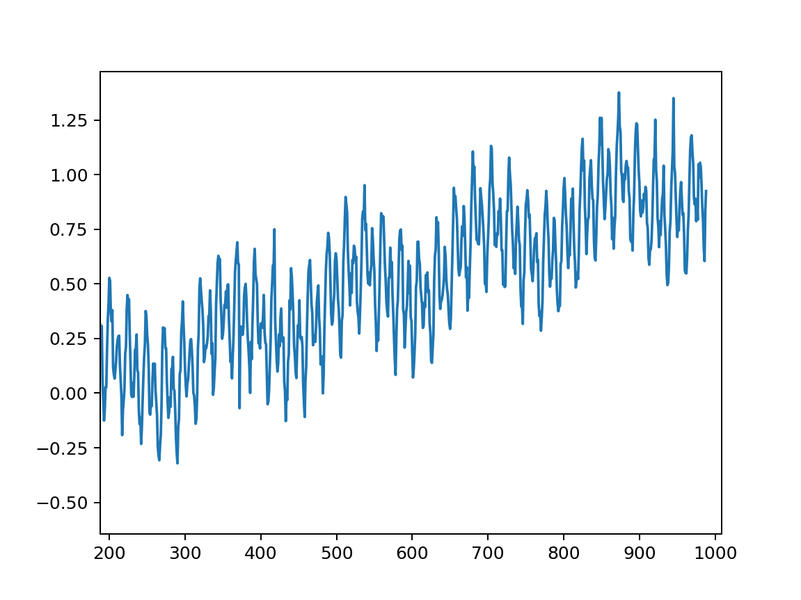
(a) Original time series

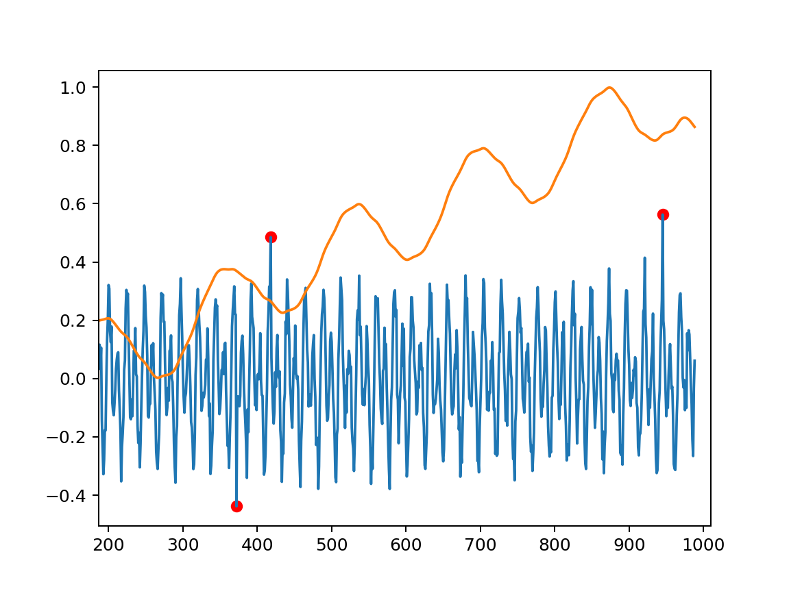
(b) Time series with decomposition

Figure 8. Examples on how decomposition helps time series anomaly detection.

5.4.2. Effect of special anomaly data augmentation.

Results in Table 4 show that, with data augmentation added, performance can be improved. The anomaly data augmentation methods above are general and not designed for specific datasets. However, if prior information of the dataset is given, special anomaly data augmentation methods can be designed to take advantage of the pattern of anomalies for further performance improvements.

To demonstrate it, one case study is summarized in Table 5 on SMAP dataset. The observation is that the first dimension of SMAP contains slow slops when anomalies appear. By utilizing this prior information, we conduct slow-slop injection on the first dimension of SMAP datasets as special anomaly data augmentation. With this specially designed data augmentation method, it can be seen in Table 5 that significant extra performance gain is achieved in the TFAD model.

Table 5. Results with slow-slop injection on first dimension of SMAP datasets as special anomaly data augmentation.

Model	Precision	Recall	F1 score
TFAD	91.90	89.32	90.32
TFAD+injection	94.04	98.36	96.09

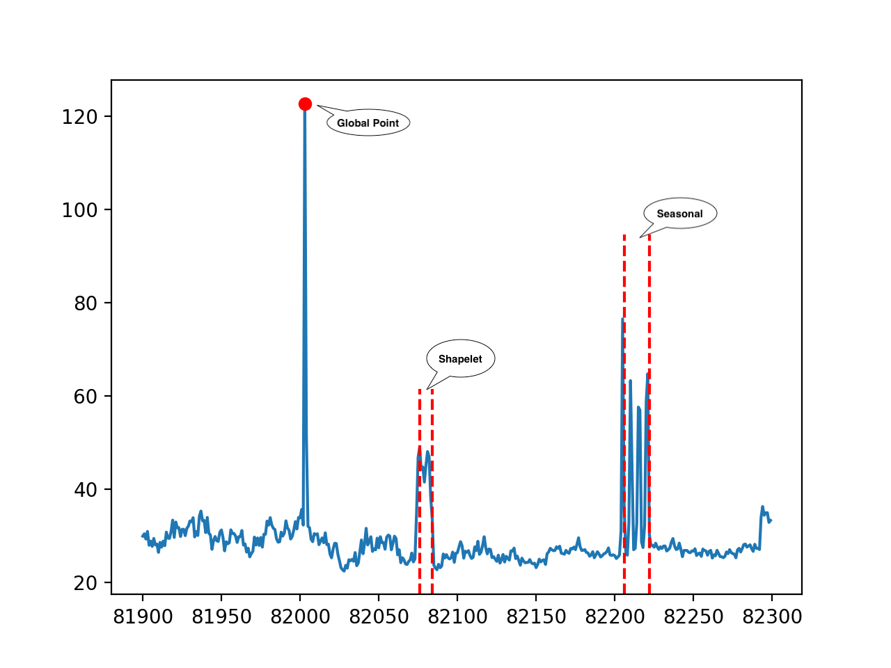
(a) Typical anomalies detected

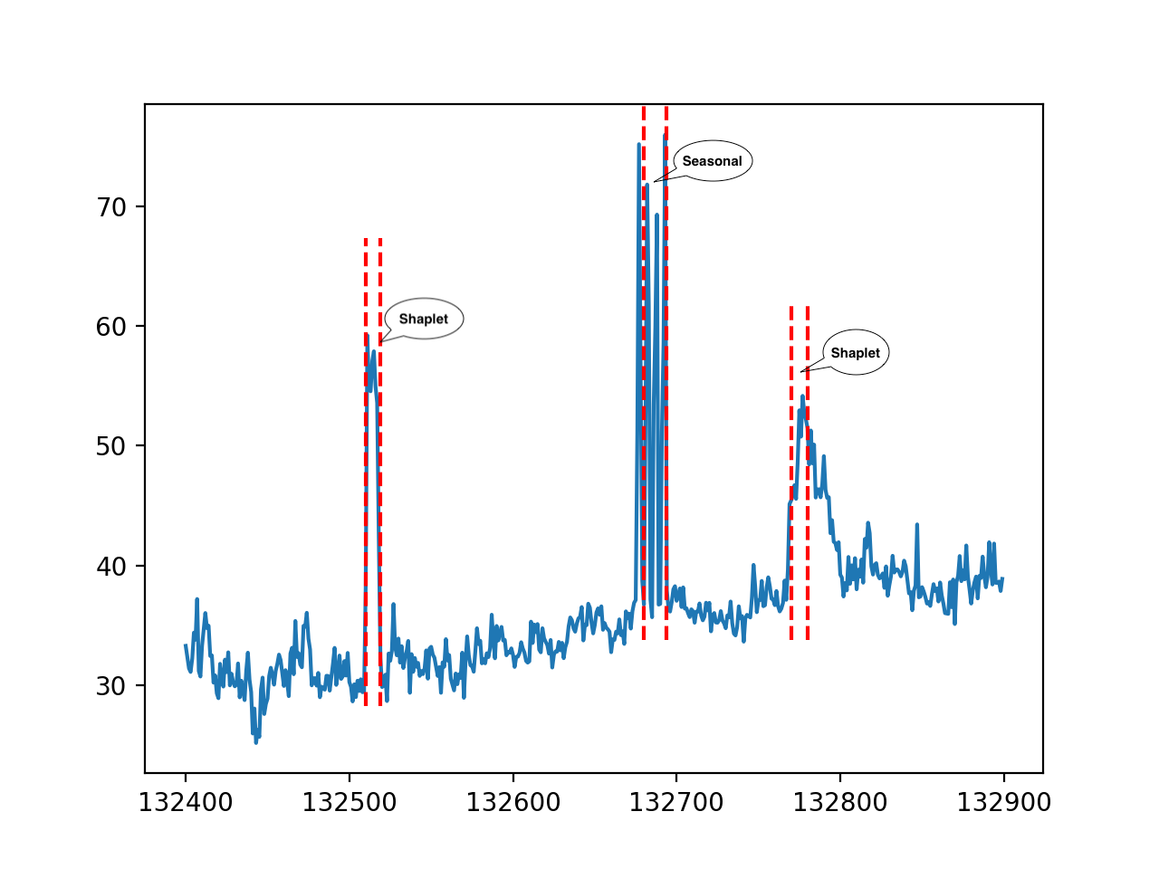
(b) Part of anomalies detected

Figure 9. Detected anomaly examples of the proposed TFAD model on KPI datasets.

5.4.3. Adaptive window size

Several typical detected anomalies of the proposed TFAD model are shown in Figure 9. In Figure 9(a), all the anomalies are detected, including point anomaly, shapelet anomaly, and seasonal anomaly. While in Figure 9(b), one interesting phenomenon is that part of the rightmost sub-sequence anomalies are not detected effectively. Considering that the anomalies in the middle and rightmost parts are near to each other and the anomalies in the middle part are more obvious than those in the rightmost part, thus when the suspect window is tested, the anomalies in the middle part change the representation of the full window and context window significantly, which will conceal the anomalies in the suspect window in the rightmost part. The adaptive window size may be a feasible solution for this problem, and we will leave it for future work.

5.4.4. Representation Network

In the TFAD model, simple temporal convolution neural (TCN) network is adopted as a representation network. We also tried the popular Transformer (Vaswani et al., 2017) based representation learning networks for time series anomaly detection, since they are widely investigated in recent time series analysis (Zhou et al., 2022; Xu et al., 2021; Zhou et al., 2021). Unfortunately, besides the high memory usage of the Transformer, the F1 score is also much less than that of TCN: F1 score of 0.59 is gained with Transformer while F1 score of 0.75 is gained with TCN on KPI dataset. The reason is that the Transformer usually works well with long time series. However, with window splitting for time series anomaly detection, the window length can not be set too long to distinguish between the full window and the context window. In this case, TCN can better model the local time series information in the window than Transformer networks. Therefore, we adopt TCN network in the TFAD model, and it not only performs quite well in anomaly detection performance but also simplifies the implementation with low memory usage.

6. Conclusion

This paper proposes a time-frequency analysis-based model (TFAD) for time series anomaly detection. Although most of the traditional and deep methods in time series anomaly detection have achieved great success, how to take advantage of the time-frequency properties of time series is not well investigated. Our design with time and frequency branches fills in this gap. Besides, time series decomposition is implemented to bring insights into the explainability of the proposed model as well as simplify the neural network design. Furthermore, we also adopt data augmentation to overcome the lack of labeled anomaly data.

Based on these considerations, the proposed TFAD with time-frequency architecture can handle the challenges of various anomalies in time series. Although no complex neural network architecture is implemented, we gain better performance than most existing deep models in time series anomaly detection. Extensive empirical studies with four benchmark datasets show that our TFAD scheme obtains a state-of-the-art performance. Furthermore, ablation studies show that TFAD gains not only higher accuracy but also lower variance for time series anomaly detection in both univariate and multivariate scenarios.

References

- (1)
- Audibert et al. (2020) Julien Audibert, Pietro Michiardi, Frédéric Guyard, Sébastien Marti, and Maria A Zuluaga. 2020. USAD: unsupervised anomaly detection on multivariate time series. In Proceedings of the 26th ACM SIGKDD International Conference on Knowledge Discovery & Data Mining. 3395–3404.
- Bai et al. (2018) Shaojie Bai, J Zico Kolter, and Vladlen Koltun. 2018. An empirical evaluation of generic convolutional and recurrent networks for sequence modeling. arXiv preprint arXiv:1803.01271 (2018).
- Blázquez-García et al. (2021) Ane Blázquez-García, Angel Conde, Usue Mori, and Jose A Lozano. 2021. A review on outlier/anomaly detection in time series data. ACM Computing Surveys (CSUR) 54, 3 (2021), 1–33.
- Bock et al. (2022) Christian Bock, François-Xavier Aubet, Jan Gasthaus, Andrey Kan, Ming Chen, and Laurent Callot. 2022. Online Time Series Anomaly Detection with State Space Gaussian Processes. arXiv preprint arXiv:2201.06763 (2022).
- Carmona et al. (2022) Chris U Carmona, François-Xavier Aubet, Valentin Flunkert, and Jan Gasthaus. 2022. Neural contextual anomaly detection for time series. In Proceedings of International Joint Conference on Artificial Intelligence (IJCAI’22).
- Chen et al. (2022b) Weiqi Chen, Wenwei Wang, Bingqing Peng, Qingsong Wen, Tian Zhou, and Liang Sun. 2022b. Learning to Rotate: Quaternion Transformer for Complicated Periodical Time Series Forecasting. In Proceedings of the 28th ACM SIGKDD Conference on Knowledge Discovery and Data Mining (Washington DC, USA) (KDD ’22). 146–156.
- Chen et al. (2022a) Zhuangbin Chen, Jinyang Liu, Yuxin Su, Hongyu Zhang, Xiao Ling, Yongqiang Yang, and Michael R Lyu. 2022a. Adaptive Performance Anomaly Detection for Online Service Systems via Pattern Sketching. arXiv preprint arXiv:2201.02944 (2022).
- Cohen (1995) Leon Cohen. 1995. Time-frequency analysis. Vol. 778. Prentice hall New Jersey.
- Competition (2018) AIOps Competition. 2018. KPI dataset. https://github.com/iopsai/iops/tree/master/phase2_env
- Dagum and Bianconcini (2016) Estela Bee Dagum and Silvia Bianconcini. 2016. Seasonal adjustment methods and real time trend-cycle estimation. Springer.
- Faloutsos et al. (2020) Christos Faloutsos, Valentin Flunkert, Jan Gasthaus, Tim Januschowski, and Yuyang Wang. 2020. Forecasting Big Time Series: Theory and Practice. In Companion Proceedings of the Web Conference 2020 (Taipei, Taiwan) (WWW ’20). 320–321.
- Freeman et al. (2021) Cynthia Freeman, Jonathan Merriman, Ian Beaver, and Abdullah Mueen. 2021. Experimental Comparison and Survey of Twelve Time Series Anomaly Detection Algorithms. Journal of Artificial Intelligence Research 72 (2021), 849–899.
- Gao et al. (2002) Bo Gao, Hui-Ye Ma, and Yu-Hang Yang. 2002. Hmms (hidden markov models) based on anomaly intrusion detection method. In Proceedings. International Conference on Machine Learning and Cybernetics, Vol. 1. IEEE, 381–385.
- Gao et al. (2020) Jingkun Gao, Xiaomin Song, Qingsong Wen, Pichao Wang, Liang Sun, and Huan Xu. 2020. RobustTAD: Robust time series anomaly detection via decomposition and convolutional neural networks. KDD Workshop on Mining and Learning from Time Series (KDD-MileTS’20) (2020).
- Garg et al. (2021) Astha Garg, Wenyu Zhang, Jules Samaran, Ramasamy Savitha, and Chuan-Sheng Foo. 2021. An Evaluation of Anomaly Detection and Diagnosis in Multivariate Time Series. IEEE Transactions on Neural Networks and Learning Systems (2021).
- Guan et al. (2016) Xudong Guan, Chong Huang, Gaohuan Liu, Xuelian Meng, and Qingsheng Liu. 2016. Mapping rice cropping systems in Vietnam using an NDVI-based time-series similarity measurement based on DTW distance. Remote Sensing 8, 1 (2016), 19.
- Gupta et al. (2013) Manish Gupta, Jing Gao, Charu C Aggarwal, and Jiawei Han. 2013. Outlier detection for temporal data: A survey. IEEE Transactions on Knowledge and data Engineering 26, 9 (2013), 2250–2267.
- Hamilton (1994) James D. Hamilton. 1994. Time Series Analysis (1 ed.). Princeton University Press. http://www.amazon.com/exec/obidos/redirect?tag=citeulike07-20&path=ASIN/0691042896
- Hendrycks et al. (2018) Dan Hendrycks, Mantas Mazeika, and Thomas Dietterich. 2018. Deep anomaly detection with outlier exposure. arXiv preprint arXiv:1812.04606 (2018).
- Hochenbaum et al. (2017) Jordan Hochenbaum, Owen S Vallis, and Arun Kejariwal. 2017. Automatic anomaly detection in the cloud via statistical learning. arXiv preprint arXiv:1704.07706 (2017).
- Hodrick and Prescott (1997) Robert J Hodrick and Edward C Prescott. 1997. Postwar US business cycles: an empirical investigation. Journal of Money, credit, and Banking (1997), 1–16.
- Hundman et al. (2018) Kyle Hundman, Valentino Constantinou, Christopher Laporte, Ian Colwell, and Tom Soderstrom. 2018. Detecting spacecraft anomalies using lstms and nonparametric dynamic thresholding. In Proceedings of the 24th ACM SIGKDD international conference on knowledge discovery & data mining. 387–395.
- Hwang et al. (2022) Won-Seok Hwang, Jeong-Han Yun, Jonguk Kim, and Byung Gil Min. 2022. Do you know existing accuracy metrics overrate time-series anomaly detections?. In Proceedings of the 37th ACM/SIGAPP Symposium on Applied Computing. 403–412.
- Jacob et al. (2020) Vincent Jacob, Fei Song, Arnaud Stiegler, Bijan Rad, Yanlei Diao, and Nesime Tatbul. 2020. Exathlon: a benchmark for explainable anomaly detection over time series. arXiv preprint arXiv:2010.05073 (2020).
- Kim et al. (2022) Siwon Kim, Kukjin Choi, Hyun-Soo Choi, Byunghan Lee, and Sungroh Yoon. 2022. Towards a Rigorous Evaluation of Time-series Anomaly Detection. AAAI (2022).
- Kiran et al. (2018) B Ravi Kiran, Dilip Mathew Thomas, and Ranjith Parakkal. 2018. An overview of deep learning based methods for unsupervised and semi-supervised anomaly detection in videos. Journal of Imaging 4, 2 (2018), 36.
- Lai et al. (2021) Kwei-Herng Lai, Daochen Zha, Junjie Xu, Yue Zhao, Guanchu Wang, and Xia Hu. 2021. Revisiting time series outlier detection: Definitions and benchmarks. In Thirty-fifth Conference on Neural Information Processing Systems Datasets and Benchmarks Track (Round 1).
- Lane et al. (1997) Terran Lane, Carla E Brodley, et al. 1997. Sequence matching and learning in anomaly detection for computer security. In AAAI Workshop: AI Approaches to Fraud Detection and Risk Management. Providence, Rhode Island, 43–49.
- Li et al. (2022) Longyuan Li, Junchi Yan, Qingsong Wen, Yaohui Jin, and Xiaokang Yang. 2022. Learning Robust Deep State Space for Unsupervised Anomaly Detection in Contaminated Time-Series. IEEE TKDE (2022).
- Muthukrishnan et al. (2004) Shan Muthukrishnan, Rahul Shah, and Jeffrey Scott Vitter. 2004. Mining deviants in time series data streams. In Proceedings. 16th International Conference on Scientific and Statistical Database Management, 2004. IEEE, 41–50.
- Parhizkar et al. (2015) Reza Parhizkar, Yann Barbotin, and Martin Vetterli. 2015. Sequences with minimal time–frequency uncertainty. Applied and Computational Harmonic Analysis 38, 3 (2015), 452–468.
- Park et al. (2018) Daehyung Park, Yuuna Hoshi, and Charles C Kemp. 2018. A multimodal anomaly detector for robot-assisted feeding using an lstm-based variational autoencoder. IEEE Robotics and Automation Letters 3, 3 (2018), 1544–1551.
- Patel et al. (2022) Dhaval Patel, Giridhar Ganapavarapu, Srideepika Jayaraman, Shuxin Lin, Anuradha Bhamidipaty, and Jayant Kalagnanam. 2022. AnomalyKiTS: Anomaly Detection Toolkit for Time Series. Proceedings of the AAAI Conference on Artificial Intelligence 36, 11 (Jun. 2022), 13209–13211.
- Ravn and Uhlig (2002) Morten O Ravn and Harald Uhlig. 2002. On adjusting the Hodrick-Prescott filter for the frequency of observations. Review of economics and statistics 84, 2 (2002), 371–376.
- Ren et al. (2019) Hansheng Ren, Bixiong Xu, Yujing Wang, Chao Yi, Congrui Huang, Xiaoyu Kou, Tony Xing, Mao Yang, Jie Tong, and Qi Zhang. 2019. Time-series anomaly detection service at microsoft. In Proceedings of the 25th ACM SIGKDD international conference on knowledge discovery & data mining. 3009–3017.
- Research (2015) Yahoo Research. 2015. A Benchmark Dataset for Time Series Anomaly Detection, https://yahooresearch.tumblr.com/post/114590420346/a-benchmark-dataset-for-time-series-anomaly. (2015).
- Rezende et al. (2014) Danilo Jimenez Rezende, Shakir Mohamed, and Daan Wierstra. 2014. Stochastic backpropagation and approximate inference in deep generative models. In International conference on machine learning. PMLR, 1278–1286.
- Robert et al. (1990) Cleveland Robert, C William, and Terpenning Irma. 1990. STL: A seasonal-trend decomposition procedure based on loess. Journal of official statistics 6, 1 (1990), 3–73.
- Ruff et al. (2021) Lukas Ruff, Jacob R Kauffmann, Robert A Vandermeulen, Grégoire Montavon, Wojciech Samek, Marius Kloft, Thomas G Dietterich, and Klaus-Robert Müller. 2021. A unifying review of deep and shallow anomaly detection. Proc. IEEE (2021).
- Ruff et al. (2018) Lukas Ruff, Robert Vandermeulen, Nico Goernitz, Lucas Deecke, Shoaib Ahmed Siddiqui, Alexander Binder, Emmanuel Müller, and Marius Kloft. 2018. Deep one-class classification. In International conference on machine learning. PMLR, 4393–4402.
- Ruff et al. (2020) Lukas Ruff, Robert A Vandermeulen, Billy Joe Franks, Klaus-Robert Müller, and Marius Kloft. 2020. Rethinking assumptions in deep anomaly detection. arXiv preprint arXiv:2006.00339 (2020).
- Schlegl et al. (2017) Thomas Schlegl, Philipp Seeböck, Sebastian M Waldstein, Ursula Schmidt-Erfurth, and Georg Langs. 2017. Unsupervised anomaly detection with generative adversarial networks to guide marker discovery. In International conference on information processing in medical imaging. Springer, 146–157.
- Shah et al. (2021) Syed Yousaf Shah, Dhaval Patel, Long Vu, Xuan-Hong Dang, Bei Chen, Peter Kirchner, Horst Samulowitz, David Wood, Gregory Bramble, Wesley M. Gifford, Giridhar Ganapavarapu, Roman Vaculin, and Petros Zerfos. 2021. AutoAI-TS: AutoAI for Time Series Forecasting. In Proceedings of the 2021 International Conference on Management of Data (Virtual Event, China) (SIGMOD ’21). 2584–2596.
- Shen et al. (2020) Lifeng Shen, Zhuocong Li, and James Kwok. 2020. Timeseries anomaly detection using temporal hierarchical one-class network. Advances in Neural Information Processing Systems 33 (2020), 13016–13026.
- Shorten and Khoshgoftaar (2019) Connor Shorten and Taghi M Khoshgoftaar. 2019. A survey on image data augmentation for deep learning. Journal of big data 6, 1 (2019), 1–48.
- Shumway et al. (2000) Robert H Shumway, David S Stoffer, and David S Stoffer. 2000. Time series analysis and its applications. Vol. 3. Springer.
- Siffer et al. (2017) Alban Siffer, Pierre-Alain Fouque, Alexandre Termier, and Christine Largouet. 2017. Anomaly detection in streams with extreme value theory. In Proceedings of the 23rd ACM SIGKDD International Conference on Knowledge Discovery and Data Mining. 1067–1075.
- Su et al. (2019) Ya Su, Youjian Zhao, Chenhao Niu, Rong Liu, Wei Sun, and Dan Pei. 2019. Robust anomaly detection for multivariate time series through stochastic recurrent neural network. In Proceedings of the 25th ACM SIGKDD international conference on knowledge discovery & data mining. 2828–2837.
- Tuli et al. (2022) Shreshth Tuli, Giuliano Casale, and Nicholas R Jennings. 2022. TranAD: Deep Transformer Networks for Anomaly Detection in Multivariate Time Series Data. In Proceedings of 48th International Conference on Very Large Databases (VLDB’22).
- Vaswani et al. (2017) Ashish Vaswani, Noam Shazeer, Niki Parmar, Jakob Uszkoreit, Llion Jones, Aidan N Gomez, Łukasz Kaiser, and Illia Polosukhin. 2017. Attention is all you need. Advances in neural information processing systems 30 (2017).
- Wen et al. (2019) Qingsong Wen, Jingkun Gao, Xiaomin Song, Liang Sun, Huan Xu, and Shenghuo Zhu. 2019. RobustSTL: A robust seasonal-trend decomposition algorithm for long time series. In Proceedings of the AAAI Conference on Artificial Intelligence (AAAI’19), Vol. 33. 5409–5416.
- Wen et al. (2021a) Qingsong Wen, Kai He, Liang Sun, Yingying Zhang, Min Ke, and Huan Xu. 2021a. RobustPeriod: Robust Time-Frequency Mining for Multiple Periodicity Detection. In Proceedings of the 2021 International Conference on Management of Data (SIGMOD’21). 2328–2337.
- Wen et al. (2021b) Qingsong Wen, Liang Sun, Fan Yang, Xiaomin Song, Jingkun Gao, Xue Wang, and Huan Xu. 2021b. Time Series Data Augmentation for Deep Learning: A Survey. In Proceedings of International Joint Conference on Artificial Intelligence (IJCAI’21). 4653–4660.
- Wen et al. (2022) Qingsong Wen, Linxiao Yang, Tian Zhou, and Liang Sun. 2022. Robust Time Series Analysis and Applications: An Industrial Perspective. In Proceedings of the 28th ACM SIGKDD Conference on Knowledge Discovery and Data Mining (Washington DC, USA) (KDD ’22). 4836–4837.
- Xu et al. (2018) Haowen Xu, Wenxiao Chen, Nengwen Zhao, Zeyan Li, Jiahao Bu, Zhihan Li, Ying Liu, Youjian Zhao, Dan Pei, Yang Feng, et al. 2018. Unsupervised anomaly detection via variational auto-encoder for seasonal kpis in web applications. In Proceedings of the 2018 world wide web conference. 187–196.
- Xu et al. (2021) Jiehui Xu, Jianmin Wang, Mingsheng Long, et al. 2021. Autoformer: Decomposition transformers with auto-correlation for long-term series forecasting. Advances in Neural Information Processing Systems 34 (2021).
- Xu et al. (2022) Jiehui Xu, Haixu Wu, Jianmin Wang, and Mingsheng Long. 2022. Anomaly Transformer: Time Series Anomaly Detection with Association Discrepancy. In International Conference on Learning Representations.
- Zhang et al. (2019) Chuxu Zhang, Dongjin Song, Yuncong Chen, Xinyang Feng, Cristian Lumezanu, Wei Cheng, Jingchao Ni, Bo Zong, Haifeng Chen, and Nitesh V Chawla. 2019. A deep neural network for unsupervised anomaly detection and diagnosis in multivariate time series data. In Proceedings of the AAAI conference on artificial intelligence (AAAI’19), Vol. 33. 1409–1416.
- Zhang et al. (2021) Yingying Zhang, Zhengxiong Guan, Huajie Qian, Leili Xu, Hengbo Liu, Qingsong Wen, Liang Sun, Junwei Jiang, Lunting Fan, and Min Ke. 2021. CloudRCA: A Root Cause Analysis Framework for Cloud Computing Platforms. In CIKM 2021.
- Zhao et al. (2020) Hang Zhao, Yujing Wang, Juanyong Duan, Congrui Huang, Defu Cao, Yunhai Tong, Bixiong Xu, Jing Bai, Jie Tong, and Qi Zhang. 2020. Multivariate time-series anomaly detection via graph attention network. In 2020 IEEE International Conference on Data Mining (ICDM). IEEE, 841–850.
- Zhou et al. (2021) Haoyi Zhou, Shanghang Zhang, Jieqi Peng, Shuai Zhang, Jianxin Li, Hui Xiong, and Wancai Zhang. 2021. Informer: Beyond efficient transformer for long sequence time-series forecasting. In Proceedings of the AAAI Conference on Artificial Intelligence (AAAI’21).
- Zhou et al. (2022) Tian Zhou, Ziqing Ma, Qingsong Wen, Xue Wang, Liang Sun, and Rong Jin. 2022. FEDformer: Frequency enhanced decomposed transformer for long-term series forecasting. In 39th International Conference on Machine Learning (ICML).
- Zong et al. (2018) Bo Zong, Qi Song, Martin Renqiang Min, Wei Cheng, Cristian Lumezanu, Daeki Cho, and Haifeng Chen. 2018. Deep autoencoding gaussian mixture model for unsupervised anomaly detection. In International conference on learning representations (ICLR’18).