Fast Functionalization with High Performance in the Autonomous Information Engine

Abstract

Mandal and Jarzynski have proposed a fully autonomous information heat engine, consisting of a demon, a mass and a memory register interacting with a thermal reservoir [Proc. Natl. Acad. Sci. U.S.A. 109, 11641 (2012)]. This device converts thermal energy into mechanical work by writing information to a memory register, or conversely, erasing information by consuming mechanical work. Here, we derive a speed limit inequality between the relaxation time of state transformation and the distance between the initial and final distributions, where the combination of the dynamical activity and entropy production plays an important role. Such inequality provides a hint that a speed-performance trade-off relation exists between the relaxation time to functional state and the average production. To obtain fast functionalization while maintaining the performance, we show that the relaxation dynamics of information heat engine can be accelerated significantly by devising an optimal initial state of the demon. Our design principle is inspired by the so-called Mpemba effect, where water freezes faster when initially heated.

Introduction.—Maxwell’s demon is a device that can measure the microstate of a closed system, thereby reducing its entropy, seemingly in violation with the second law Maxwell and Pesic (2001). Discussions on this thought experiment raged through most of the twentieth century Smoluchowski (1927); Szilard (1929); Brillouin (1951); Penrose (2005); Feynman et al. (2011) and found a full resolution with the works of Landauer and Bennett Landauer (1961); Bennett (1982). Crucial point to understand the problem is the fact that the demon needs to store information about the gas particles and this involves increasing the information entropy of the memory registers. Later, deleting this information requires an increase in entropy such that the second law is restored Maruyama et al. (2009). Due to experimental advances, it is nowadays possible to control systems down to the nanoscale, making it possible to realize Maxwell’s demon in the laboratory Serreli et al. (2007); Bérut et al. (2012); Toyabe et al. (2010); Koski et al. (2014a, b, 2015); Vidrighin et al. (2016); Cottet et al. (2017); Kumar et al. (2018); Masuyama et al. (2018); Ribezzi-Crivellari and Ritort (2019); Paneru et al. (2020). Maxwell’s "intelligent" demon provides an excellent arena for studying the thermodynamic framework of information processing Zurek (1989); Maruyama et al. (2009); Hosoya et al. (2011). Theoretical research on models fall into two categories: autonomous Mandal and Jarzynski (2012); Mandal et al. (2013); Barato and Seifert (2014); Horowitz and Esposito (2014); Strasberg et al. (2017); Joseph and Kiran (2021); Lu and Jarzynski (2019) and feedback control loops Barato and Seifert (2014); Horowitz and Esposito (2014); Strasberg et al. (2017); Quan et al. (2006); Abreu and Seifert (2011); Ribezzi-Crivellari and Ritort (2019).

Recently, physicists have devised a series of autonomous models without the participation of any "intelligent" demon, which can achieve Maxwell’s original vision and obtain results that are consistent with the predictions of Landauer’s principle Mandal and Jarzynski (2012); Mandal et al. (2013); Barato and Seifert (2014); Horowitz and Esposito (2014); Strasberg et al. (2017); Joseph and Kiran (2021); Lu and Jarzynski (2019). The construction of autonomous information heat engines or erasers not only helps to understand the basic concepts of information thermodynamics, but also has important application prospects. Particularly, Mandal and Jarzynski proposed a fully autonomous information heat engine (IHE) setup Mandal and Jarzynski (2012). After a certain relaxation time to enter the functional state, the IHE converts thermal energy into mechanical work by writing information to a memory register, rectifying thermal fluctuations, or conversely, by consuming mechanical work to (partially) erase the information on the memory register. Going a step further, they also considered an autonomous information refrigerator (IR) model Mandal et al. (2013). Similar to the IHE model, the refrigerator utilizes thermal fluctuations to transfer heat from a low temperature thermal reservoir to a high temperature, or acts as an eraser to reduce the information on the memory register after a finite relaxation interval to function. The performance of the autonomous IHE/IR is measured by the average production, which quantifies the rectification of the bits. A natural thought is that one may expect that an efficient model can quickly enter the functional state with high-performance. Therefore, how to design the IHE to achieve fast functionalization while maintaining high production is of great importance.

In this letter, we analyze both the speed (relaxation time to functional state) and the performance (average production) of autonomous IHE model. An inequality related the rate of the state transformation to the distance between two probability distributions has been derived to claim that there is a speed-performance trade-off relation between the relaxation time and the production, highlighting that the IHE cannot be functionalized quickly with high production for fixed entropy production. To overcome this limitation, we are committed to develop a design strategy that allows the IHE to move quickly into an highly efficient state. Remarkably, we show that the IHE can always reach the stationary functional state at a remarkable faster pace by specially preparing the demon’s initial state, which is reminiscent of the Markovian Mpemba effect Aristotle and Aristotle (1933); Mpemba and Osborne (1969); Lu and Raz (2017); Klich et al. (2019); Gal and Raz (2020); Carollo et al. (2021); Kumar and Bechhoefer (2020); Lasanta et al. (2017); Baity-Jesi et al. (2019); Gijón et al. (2019); Torrente et al. (2019); Chétrite et al. (2021); Vadakkayil and Das (2021); Yang and Hou (2020); Busiello et al. (2021); Schwarzendahl and Löwen (2021); Santos and Prados (2020); Biswas et al. (2022).

Model.—We start by introducing a modified IHE setup proposed by Mandal and Jarzynski, as illustrated in Fig. 1. In general, the IHE model has $k$-state demon that interacts with a mass, a thermal reservoir with temperature $T$, and a stream of bits (labeled $0$ and $1$), which acts as memory registers. The demon is initially set up in contact with another thermal reservoir with temperature $T_{\text{ini}}$ to reach equilibrium, and then it is coupled to the memory registers, constituting a $2k$-states composite system. At any instant in time, the bit stream moves through the demon in a given sequence written in advance at a constant speed. After interacting with the demon for a fixed time interval $\tau$, the bit moves forward, and a new bit comes in. The demon transfers randomly between $k$ states, and the bit can transfer together with the demon from state 0 (1) to 1 (0). Net differences between the clockwise (CW) and counterclockwise (CCW) cyclic transition will cause the demon to display directional rotation and lift the mass.

Take the 3-state model ($k=3$, labeled $A$, $B$ and $C$) for example shown in Fig. 1 (a), where the states $B$ and $A/C$ are characterized by an energy difference $\Delta E=E_{u}-E_{d}$ with $E_{B}=E_{u}$ and $E_{A}=E_{C}=E_{d}$ [c.f. Fig. 1 (b)]. It can be defined that the transition in the $A\rightarrow B\rightarrow C\rightarrow A$ direction is CW, and the transition in the opposite direction is CCW. If the demon is uncoupled to the bit, it can only jump between states $A$ and $B$, and $B$ and $C$, which means there is no net cycle and the mass can not be lifted. However, if the demon interacts with the bit, they will together form a composite system with six states ($A_{0}$, $A_{1}$, $B_{0}$, $B_{1}$, $C_{0}$, $C_{1}$). Thereupon, the demon is allowed to transfer from $C$ to $A$ if the bit flips from $0$ to $1$ simultaneously, and vice versa [c.f. Fig. 1(c)], which means that the net flux of cycle can emerge due to such cooperative transitions with the help of the bit stream. The average number of net cycles can be identified as the production, which is the key performance of IHE. The incoming bit stream of the IHE contains a mixture of $0$’s and $1$’s with fixed probabilities $p_{0}$ and $p_{1}$, which are statistically independent respectively. The evolution of the probability distribution in every interval can be separated into two stages: (i) the Markovian evolution of composite $2k$-state distribution governed by transition matrix $\{R_{ij}\}$, and (ii) the projection process at the end of every interval, which eliminates the correlations between the $k$-state system and the bit. For a finite interval, the IHE will relax to a periodic steady state for a large enough interval number. Let $\delta=p_{0}-p_{1}$ denotes the proportional excess of $0$’s among incoming bits initially. Once the demon has reached its periodic steady state, let $p_{0}^{\prime}$ and $p_{1}^{\prime}$ denote the fractions of $0$’s and $1$’s in the outgoing bit stream, and $\delta^{\prime}=p_{0}^{\prime}-p_{1}^{\prime}$. The circulation as a measure of the average production of $1$’s per interaction interval in the outgoing bit stream can then be defined as

$$\Phi=p_{1}^{\prime}-p_{1}=\frac{\delta-\delta^{\prime}}{2}.$$ (1)

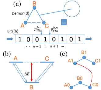
Figure 1: The information heat engine (IHE) setup. (a) The three-state demon interacts with a sequence of bits, a mass and a reservoir. (b) Schematic depiction of the demon. The state of the demon is indicated by an arrow pointing in one of the directions. The states $B$ and $A/C$ are characterized by an energy difference $\Delta E=E_{u}-E_{d}$ with $E_{B}=E_{u}$ and $E_{A}=E_{C}=E_{d}$. (c) Network depiction of the composite $6$-state system, showing allowed transitions. The edge connecting $A_{1}$ and $C_{0}$ originates from the coupling between demons and bits.

Further elaborating the evolution of composite $2k$-state system, we introduce the transition matrix $\mathcal{\bm{\mathcal{T}}=\mathcal{\bm{\mathcal{T}}}}_{k\times k}$ whose element $T_{\mu\nu}$ represents the probability for the demon to be in state $\mu$ at the end of an interaction interval, given that it was in state $\nu$ at the start of the interval. Let $\bm{p}_{\text{INI}}^{d,n}/\bm{p}_{\text{FIN}}^{d,n}$ ($\bm{p}_{\text{INI}}^{b,n}/\bm{p}_{\text{FIN}}^{b,n}$) denote the distribution of the demon (bit) at the start/end of the $n$-th interaction interval, and $\bm{p}_{\text{INI}}^{b,0}=(p_{0},p_{1})$. The evolution of the demon over many intervals is given by repeated application of the matrix $\mathcal{\bm{\mathcal{T}}}$ [SM]. Because $\mathcal{\bm{\mathcal{T}}}$ is a positive transition matrix, the demon evolves to a periodic steady state,

$$\lim_{n\to\infty}\bm{p}_{\text{INI}}^{d,n}=\lim_{n\to\infty}\mathcal{\bm{\mathcal{T}}}^{n}\bm{p}_{\text{INI}}^{d,0}=\bm{p}_{\text{INI}}^{d,ps}.$$ (2)

The unique periodic steady state can be obtained by solving $\mathcal{\bm{\mathcal{T}}}\bm{p}_{\text{INI}}^{d,ps}=\bm{p}_{\text{INI}}^{d,ps}$, which is just the functional state of the IHE which can produce anomalous work stably. Meanwhile, the bit distribution at the end of the $n$-th interaction interval, $\bm{p}_{\text{FIN}}^{b,n}$, also converges to a periodic steady state as $\lim_{n\to\infty}\bm{p}_{\text{FIN}}^{b,n}=\bm{p}_{\text{FIN}}^{b,ps}=(p_{0}^{\prime},p_{1}^{\prime})$. Nevertheless, compared to the evolution of demon distribution [Eq. (2)], the evolution of bit distribution cannot be simply described by a propagator due to the bit reset operation at the start of each interval. For the 3-state model introduced above [c.f. Fig. 1], the exact expression of the periodic steady state $\bm{p}_{\text{INI}}^{d,ps}$ and average production $\Phi$ can be obtained by solving the evolution theoretically, which can be found in the Supplemental Material [SM].

Speed-performance trade-off relation.— As stated above, the demon will go through a certain number of time intervals before reaching the periodic steady state, and the relaxation time for the demon to move from an initial state to the functional state is another crucial feature besides the production. In the following, we turn to analyze the relationship between the relaxation time and average production. We use the $L^{1}$-norm to measure the statistical distance of two probability distributions $\bm{p}$ and $\bm{q}$, i.e., the total variation distance reads as $D(\bm{p},\bm{q})=\left\|\bm{p}-\bm{q}\right\|=\sum_{i}\left|p_{i}-q_{i}\right|$. When the demon reaches the periodic steady state, the composite system reaches the functional state simultaneously. We assume that there exists a critical interval number $N_{c}=N_{c}(d)$ satisfying $D(\bm{p}_{\text{FIN}}^{b,N_{c}},\bm{p}_{\text{FIN}}^{b,\infty})\leq d$, which is expected to be proportional to the relaxation time $\tau_{c}=N_{c}\tau$ when the cut-off parameter $d$ is sufficiently small. Thus, it is important to analyze the distance between the bit distribution of the $n$-th interval $\bm{p}_{\text{FIN}}^{b,n}$ and the steady one $\bm{p}_{\text{FIN}}^{b,\infty}$ at the end of each period, i.e., $D(\bm{p}_{\text{FIN}}^{b,n},\bm{p}_{\text{FIN}}^{b,\infty})$. The average production are connected to the distance between the initial bit state $\bm{p}_{\text{INI}}^{b,0}=(p_{0},p_{1})$ and the final periodic steady state $\bm{p}_{\text{FIN}}^{b,\infty}=(p_{0}^{\prime},p_{1}^{\prime})$ as $2\Phi=D(\bm{p}_{\text{INI}}^{b,0},\bm{p}_{\text{FIN}}^{b,\infty})$. Then, we perform an approximation that $2\Phi=D(\bm{p}_{\text{INI}}^{b,0},\bm{p}_{\text{FIN}}^{b,\infty})\approx D(\bm{p}_{\text{FIN}}^{b,0},\bm{p}_{\text{FIN}}^{b,\infty})$, assuming that the difference between the initial bit state and final one of the first interval is small. This assumption is based on the intuition that the change of the bit state in a single interval will not be particularly large.

As mentioned above, the evolution of the bit is non-Markovian (can not be described by a propagator), so it is difficult to explore the convergence of the bit distribution $\bm{p}_{\text{FIN}}^{b,n}$, i.e., $D(\bm{p}_{\text{FIN}}^{b,n},\bm{p}_{\text{FIN}}^{b,\infty})$. However, the evolution of demon distribution is easier to capture, so we develop an information-theoretical relation between the distance function of the bit and demon to face this difficulty, which reads

$$D(\bm{p}_{\text{FIN}}^{b,n},\bm{p}_{\text{FIN}}^{b,0})\leq D(\bm{p}_{\text{INI}}^{d,n},\bm{p}_{\text{INI}}^{d,0})$$ (3)

for any interval number $n$ [SM]. Eq. (3) shows that the distance between final bit distribution of the $n$-th interval and initial one is always smaller than the distance between initial demon distribution of the $n$-th interval and initial one, which serves as a hierarchy of the distance function between the distribution of demon and bit. Physically, such hierarchical relation can be interpreted as the bit distance is the projection of the demon distance in lower dimensions, determined by the unusual dynamics of IHE [SM]. Based on Eq. (3), the relationship between the average production and the demon distance can be obtained as

$$2\Phi\lesssim D(\bm{p}_{\text{INI}}^{d,0},\bm{p}_{\text{INI}}^{d,\text{$\infty$}}).$$ (4)

Without loss of generality, we further assume the transition matrix $\mathcal{\mathcal{\bm{\mathcal{T}}}}$satisfies the detailed balance condition Mandal and Jarzynski (2012). By using the hierarchical structure, a speed limit inequality between the critical interval number $N_{c}$ (i.e., the relaxation time) and average production can be obtained as $\Phi$

$$N_{c}\geq N_{\text{SL}}=\frac{\Phi}{\sqrt{\frac{1}{2}\text{$\dot{\Sigma}_{N_{c}}$}\cdot\langle A\rangle_{N_{c}}}}.$$ (5)

Here, $\Sigma_{N_{c}}\equiv\sum_{n=0}^{N_{c}}\Delta_{n}S$ is the total entropy production with $\Delta_{n}S\equiv\sum_{i,j}\mathcal{T}_{ij}p_{\text{INI},j}^{d,n}\ln\left(\mathcal{T}_{ij}p_{\text{INI},j}^{d,n}/\mathcal{T}_{ji}p_{\text{INI},i}^{d,n}\right)$ the entropy production for the $n$th interaction interval, and $\dot{\Sigma}_{N_{c}}=\Sigma_{N_{c}}/N_{c}$ is its average rate. The dynamical activity $A(n)=\sum_{i\neq j}\mathcal{T}_{ij}p_{\text{INI},j}^{d,n}$ and its time average $\langle A\rangle_{N_{c}}=N_{c}^{-1}\sum_{n=0}^{N_{c}}A(n)$ quantify how frequently jumps between different states occur, i.e., the time scale of the system Shiraishi et al. (2018); Lecomte et al. (2007); Garrahan et al. (2007); Baiesi et al. (2009a, b); Maes (2017); Di Terlizzi and Baiesi (2018). The novelty of this nontrivial relation reveals that there exists a speed-performance trade-off between the relaxation time and average production, highlighting that the IHE cannot be functionalized quickly with high production for fixed entropy production. The structure of Eq.(5) also reminds us of the conventional quantum speed limit Mandelstam and Tamm (1991); Fleming (1973); Anandan and Aharonov (1990); Margolus and Levitin (1998); Pfeifer (1993); Taddei et al. (2013); del Campo et al. (2013); Deffner and Lutz (2013); Pires et al. (2016); Funo et al. (2017); Deffner (2017), which is an important issue relevant to broad research fields including quantum control theory and have been extended to the case of classical dynamics recently Shanahan et al. (2018); Okuyama and Ohzeki (2018); Ito (2018); Shiraishi et al. (2018); Shiraishi and Saito (2019); Nicholson et al. (2020); Ito and Dechant (2020); Van Vu et al. (2020); Gupta and Busiello (2020); Yoshimura and Ito (2021). In addition, we state that a series of similar inequalities can be obtained and the result of Eq. (5) can be further improved. Among them, the tightest form reads

$$N_{c}\geq N_{TSL}=\frac{2\Phi}{\dot{\Sigma}_{N_{c}}}\cdot f\left(\frac{\dot{\Sigma}_{N_{c}}}{2\langle A\rangle_{N_{c}}}\right).$$ (6)

Eqs. (5) and (6) constitute our first important result. Here, $f(x)$ is the inverse function of $x\tanh(x)$, and the concavity property of the function $(x^{2}/y)f(x/y)^{-2}$ ensures that Eq. (6) is tighter than Eq. (5) with $N_{c}\geq N_{TSL}\geq\max\left\{N_{\text{SL}},\Phi/\langle A\rangle_{N_{c}}\right\}$ Vo et al. (2022); Lee et al. (2022). The detailed derivation has been provided in the Supplemental Material (SM). Finally, we reiterate that the speed limit holds for the detailed balance case and declare that an analogous relation for the general case without detailed balance condition can also be obtained in a similar way, where the excess entropy production Hatano and Sasa (2001) plays a substitute role as the conventional total entropy production Shiraishi et al. (2018).

Here, we demonstrate the speed limit inequality with the $3$-state IHE model introduced above, c.f. Fig. 1. The control parameters in this model are the weight parameter $\epsilon$, excess of the incoming bit $\delta$ and the time interval $\tau$. More detailed descriptions have been provided in the SM [SM]. By setting the cut-off parameter $d=10^{-6}$, the critical interval number $N_{c}$, entropy production rate $\dot{\Sigma}_{N_{c}}$ and the average dynamical activity $\langle A\rangle_{N_{c}}$ can be obtained from numerically operating the convergence of demon state, $\bm{p}_{\text{INI}}^{d,n}=\mathcal{\bm{\mathcal{T}}}^{n}\bm{p}_{\text{INI}}^{d,0}$. Meanwhile, the average production $\Phi$ can be obtained from the exact expression [SM]. We depict the critical interval number $N_{c}$ (black circles), the speed limit bound $N_{SL}$ (orange down triangles) and its tighter form $N_{TSL}$ (blue up triangles) as functions of the average production $\Phi$ by varying $\delta$ with fixed $\tau=1.0$ and $\epsilon=0.1$ in Fig. 2. Our speed limits Eq.(5) and Eq.(6) are valid, which provides the hint of the speed-performance trade-off and do reasonable job of predicting the critical functionalization interval of the IHE.

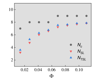
Figure 2: Demonstration of the speed-limit inequalities for the $3$-state model. The critical interval number $N_{c}$ (black circles), speed limit bound $N_{\text{SL}}$ (orange down triangles) and its tighter form $N_{TSL}$ (blue up triangles) have been shown as functions of the average production $\Phi$, where $f(x)$ is the inverse function of $x\tanh(x)$. Both Eqs. (5) and (6) have been verified. Different points are obtained from varying $\delta$ with fixed $\tau=1.0$ and $\delta=0.1$.

Fast functionalization.—Due to the speed-performance trade-off relation, we are motivated to find a design strategy to speed up the functionalization while maintaining the average production. To this goal, we analyze the relaxation modes and timescales based on the framework of spectral decomposition. As mentioned above, the matrix $\mathcal{\bm{\mathcal{T}}}$ governs the evolution of the system. The eigenvalues of $\mathcal{\bm{\mathcal{T}}}$ is related to the timescale for different dynamical modes, which can be numbered in a descending order: $1=\mu_{1}>\left|\mu_{2}\right|\geq\left|\mu_{3}\right|\geq...$ (here, we assume that $\mu_{1}$ is not degenerate). Accordingly, the right $\bm{R}_{i}$ and left eigenvectors $\bm{L}_{i}$ for an eigenvalue $\mu_{i}$ correspond to the $i$-th dynamical modes, which read $\mathcal{\mathcal{\bm{\mathcal{T}}}}\bm{R}_{i}=\mu_{i}\bm{R}_{i}$ and $\bm{L}_{i}^{\text{T}}\mathcal{\mathcal{\bm{\mathcal{T}}}}=\mu_{i}\bm{L}_{i}^{\text{T}}$, respectively. The right eigenvector $\bm{R}_{1}$ for the principal eigenvalue $1=\mu_{1}$ is the functional periodic steady state, $\bm{R}_{1}=\bm{p}_{\text{INI}}^{d,ps}$, and its corresponding left eigenvector is the identity. The spectral decomposition allows us to expand any probability distribution as a linear combination of the eigenvectors. Particularly, for the initial state $\bm{p}_{\text{INI}}^{d,0}$, it can be written as

$$\bm{p}_{\text{INI}}^{d,0}=\bm{p}_{\text{INI}}^{d,ps}+\sum_{i>1}d_{i}\bm{R}_{i},$$ (7)

where the corresponding overlap coefficient between the initial probability and the $i$-th left eigenvector $\bm{L}_{i}^{\text{T}}$ is

$$d_{i}=\frac{\bm{L}_{i}^{\text{T}}\cdot\bm{p}_{\text{INI}}^{d,0}}{\bm{L}_{i}^{\text{T}}\cdot\bm{R}_{i}}.$$ (8)

During the relaxation process, the initial demon distribution of the $n$-th time interval, $\bm{p}_{\text{INI}}^{d,n}$, can then be obtained as

$$\bm{p}_{\text{INI}}^{d,n}=\mathcal{\bm{\mathcal{T}}}^{n}\bm{p}_{\text{INI}}^{d,0}=\bm{p}_{\text{INI}}^{d,ps}+\sum_{i>1}d_{i}\mu_{i}^{n}\bm{R}_{i}.$$ (9)

We once again emphasize that the eigenvectors can be interpreted as dynamical modes that transport probability density from one part of the conformational space to another, and the modules of the eigenvalues give the relaxation rates of all the modes which has been excited. From Eq.(9), we find that the second eigenvalue $\left|\mu_{2}\right|$ determines the spectral gap, characterizing the longest timescale of the relaxation, and $\bm{R}_{2}$ is in fact the slowest decaying mode of the demon. Hence, the probability distribution (9) can be approximated after a long time as $\mathcal{\bm{\mathcal{T}}}^{n}\bm{p}_{\text{INI}}^{d,0}\approx\bm{p}_{\text{INI}}^{d,ps}+d_{2}\mu_{2}^{n}\bm{R}_{2}$.

The explicit expression of the distance between the initial demon distribution of the $n$-th time interval and the functional state can be measured by the $L^{1}$-norm, which reads $\left\|\mathcal{\bm{\mathcal{T}}}^{n}\bm{p}_{\text{INI}}^{d,0}-\bm{p}_{\text{INI}}^{d,ps}\right\|=\sum_{i>1}d_{i}\left|\mu_{i}\right|_{q}^{n}\left\|R_{i}\right\|$. Since the second eigenvalue $\left|\mu_{2}\right|$ determines the decaying process dominantly, the relaxation timescale $\tau_{c}\equiv N_{c}\tau$ can be typically characterized as $\tau_{c}\sim\tau_{2}=-1/\text{$\ln$}\left|\mu_{2}\right|$, i.e., the critical interval number $N_{c}$ is proportional to the relaxation timescale as $N_{c}\propto\tau_{2}$ for a non-degenerate system. Further, it can be found that the decaying rate of process depends mostly on the overlap between between the initial probability and the dominant mode $d_{2}$. A smaller $d_{2}$ implies that the dominant mode are excited moderately and will induce a faster relaxation. Such mechanism is in spirit similar to some kind of anomalous relaxation referred as the Markovian Mpemba effect Lu and Raz (2017), where initiating the system at a hot temperature results in faster cooling down than any colder temperature when the system is coupled to a cold bath. Generally, the dynamics of the demon overlaps with all decaying modes, particularly the slowest one. However, it can be observed that the slowest mode can be completely depopulated initially if there exists an equilibrium initial demon distribution $\bm{\pi}_{\text{INI}}^{d}$ satisfying $d_{2}|_{\bm{p}_{\text{INI}}^{d,0}=\bm{\pi}_{\text{INI}}^{d}}=0$, i.e.,

$$\bm{L}_{2}^{\text{T}}\cdot\bm{\pi}_{\text{INI}}^{d}=0,$$ (10)

Reasonably, for the IHE, the specific initial state $\bm{\pi}_{\text{INI}}^{d}=\bm{\pi}_{\text{INI}}^{d}(T_{opt})$ can be obtained by preparing the demon in a thermal reservoir with an optimal temperature $T_{\text{ini}}=T_{\text{opt}}\neq T$. To be specific, by preparing the demon’s initial state $\bm{p}_{\text{INI}}^{d,0}=\bm{\pi}_{\text{INI}}^{d}(T_{opt})$ orthogonal to $\bm{L}_{2}$, the state converges at a shorter timescale $\tau_{3}=-1/\text{$\ln$}\left|\mu_{3}\right|$, which is in favor of a remarkable faster pace of the relaxation. Particularly, for the 3-state IHE with $\bm{L}_{2}=(L_{21},L_{22},L_{23})$, the optimal temperature can be solved as [SM]

$$T_{\text{opt}}/\Delta E=\left[k_{b}\ln(-\frac{L_{21}+L_{23}}{L_{22}})\right]^{-1},$$ (11)

which is the second main result of our paper. Here, $k_{b}$ is the Boltzmann constant. The basic mechanism underpinning such phenomenon is reminiscent of the strong Mpemba effect (SME) Klich et al. (2019), which has been verified by experiments in colloidal systems Kumar and Bechhoefer (2020). The set of initial states whose projection along $\bm{L}_{2}^{\text{T}}$ vanishes will identify a ($k-2$)-manifold which is referred to as the strong Mpemba space (SM space), suggesting that the SME can only exist in the model with more than two states. Although the relationship between the energy landscape and approach to stationary state is generally complex and volatile, the SME shows that special initial state setups will induce a shortcut in relaxation, providing a useful recipe for the design of high-quality information machine.

Figure 3: Demonstration of the strong Mpemba effect (SME). Optimal initial temperatures of demon $T_{opt}/\Delta E$ [obtained from Eq. (11)] are plotted as a function of the weighted parameter $\epsilon$ (the red line). Parameter $\tau=3.0$ and $\delta=0.5$ are fixed. Inset shows the critical relaxation time $N_{c}\tau$ (green squares) and the overlap between between the initial probability and the dominant mode $d_{2}$ (the blue line) as a function of the initial demon temperature $T_{ini}/\Delta E$ for $\epsilon=0.4$. When $d_{2}(T_{opt})=0$, the relaxation time reaches its minimum and the SME occurs.

In the following, we illustrate that the 3-state IHE model allows us to demonstrate how the SME controls the timescale for the approach to the functional state. In Fig. 3, the optimal initial temperatures of demon $T_{opt}/\Delta E$, which can be theoretically predicted from Eq. (11), have been plotted as a function of the weighted parameter $\epsilon$ (the red line) with $\tau=3.0$ and $\delta=0.5$. Also, the critical relaxation time $N_{c}\tau$ (green squares) can be numerically calculated, and the overlap between between the initial probability and the dominant mode $d_{2}$ (the blue line) can be obtained from the theoretical result of the spectral decomposition of $\mathcal{\bm{\mathcal{T}}}$ [SM]. Both $N_{c}\tau$ and $d_{2}$ have been depicted as a function of the initial demon temperature $T_{ini}/\Delta E$ for fixed $\epsilon=0.4$ in the inset of Fig. 3. Remarkably, it can be found that the relaxation process is typically accelerated for the certain initial demon temperature where the SME occurs with $d_{2}(T_{opt})=0$, demonstrating the applicability of our design principle.

Discussion.—In summary, we have derived speed limit inequalities for the case of information machine. These results can be useful for understanding trade-off relation between the speed of relaxation to the functional state and the average production. To address this issue, we have presented a design principle to shorten the timescale for the approach to the functional state. Without sacrificing the production, speed of relaxation can be accelerated by rationally designing the initial state of the demon so that the slowest relaxation mode is no longer excited. We have demonstrated our results by numerical verification.

Besides the speed limit we derived, other techniques might also be hopeful to reveal such relation, such as the thermodynamic uncertainty relation for arbitrary initial states Liu et al. (2020) and the information geometry Ito (2018); Ito and Dechant (2020). And, the trade-off between speed and performance may be widespread in other systems, such as periodic heat engine. Since the existence of SME is robust to perturbations and can be observed even in the thermodynamic limit Klich et al. (2019), we believe that the proposed design principle is readily accessible in experiments. Finally, we also suggest another interesting avenue deserving special attention is that the stochastic resetting mechanism can further improve the speed and performance of information engine Bao et al. (2022).

Supplementary Material for “Faster Functionalization with High Performance in the Autonomous Information Engine”

Appendix A Details of the model

Here, we introduce the modified IHE model in more details, as shown in Fig. 1. As mentioned in the main text, the IHE model has $k$-state (here, $k=3$) demon that interacts with: a thermal reservoir, a mass that can be lifted or lowered, and a stream of bits (labeled $0$ and $1$). When the bit moves forward, the demon transitions between the $A$, $B$ and $C$ states simultaneously. When uncoupled to the bit, the demon can jump between states $A$ and $B$, and $B$ and $C$. With the help of the bit stream, the demon and bit together form a composite system with six states, $A_{0},\dots,C_{1}$, which allows the transitions between $A$ and $C$ for the demon. Precisely, when the demon interacts with the bit, the demon can transition from $C$ to $A$ if the bit flips from $0$ to $1$ simultaneously, and vice versa, as shown in Fig. 1(c). The frequency difference between the CW transition and the CCW transition will cause the demon to display directional rotation.

We consider a positive positive external load $f=mg\Delta h/k_{b}T>0$ ($T$ is the temperature of the thermal reservoir and $k_{b}$ is Boltzmann constant), assuming that the mass $m$ is lifted by $\Delta h$ every time the demon makes a transition $C\rightarrow A$, and lowered with $A\rightarrow C$. The transition rates with detailed balance can be written as

$$\frac{R_{A,B}}{R_{B,A}}=\frac{R_{C,B}}{R_{B,C}}=e^{-\Delta E/k_{b}T},$$ (12)

and

$$\frac{R_{A_{1},C_{0}}}{R_{C_{0},A_{1}}}=e^{-f}.$$ (13)

For convenience, we set the $\Delta E\ll T\sim mg\Delta h$ so that $R_{ij}=1$ for all transition rates except $R_{A_{1},C_{0}}$ and $R_{C_{0},A_{1}}$. In particular, when the demon interacts with a fixed bit for a long enough time, both of them will reach equilibrium simultaneously, whose distribution read

$$p_{i,\>i\in\{A_{0},B_{0},C_{0}\}}^{eq}=\frac{e^{f}}{Z},\qquad p_{i,\>i\in\{A_{1},B_{1},C_{1}\}}^{eq}=\frac{1}{Z}$$ (14)

with $Z=3(1+e^{f})$. For simplicity, a weight parameter $\epsilon$ is defined to describe the difference between the equilibrium probabilities for the bit after summing over the states of the demon,

$$\epsilon\equiv p_{0}^{eq}-p_{1}^{eq}=\tanh(\frac{f}{2}).$$ (15)

We assume that the incoming bit stream contains a mixture of $0$’s and $1$’s, with probabilities $p_{0}$ and $p_{1}$, respectively, with no correlations between bits. As stated in the main text, $\delta=p_{0}-p_{1}$ denotes the proportional excess of 0’s among incoming bits. The evolution of the composite six-state system in every interval can be separated into two stages: (i) the dynamic evolution governed by transition rates $\{R_{ij}\}$, and (ii) the projection process at the end of every interval, which eliminates the correlations between the three-state system and the bit. For a finite $\tau$, the IHE will reach a periodic steady state for large enough period number. Once the demon has reached its periodic steady state, let $p_{0}$ and $p_{1}$ denote the fractions of $0$’s and $1$’s in the outgoing bit stream, and let $\delta^{\prime}=p_{0}^{\prime}-p_{1}^{\prime}$ denote the excess of outgoing $0$’s. The circulation as a measure of the average production of $1$’s per interaction interval in the outgoing bit stream, which is the key performance of the engine, can is defined as $\Phi=p_{1}^{\prime}-p_{1}=\left(\delta^{\prime}-\delta\right)/2$ [c.f. Eq. (1) in the main text].

Appendix B Derivation of the speed limit

B.1 Solving for the average production

Firstly, we show the exact expression of average production, which can be obtained by solving the periodic steady state as Mandal and Jarzynski (2012)

$$\Phi(\delta,\epsilon;\tau)=\frac{\delta-\epsilon}{2}\left[1-K(\tau)+\frac{\tau\delta}{6}J(\tau,\epsilon\delta)\right]$$ (16)

with

$$K(\tau)=e^{-2\tau}\frac{\left(1+8\alpha+4\sqrt{3}\beta\right)-\left(2+7\alpha+4\sqrt{3}\beta\right)e^{-2\tau}}{3-\left(2+\alpha\right)e^{-2\tau}}$$ (17)

and

$$J(\tau,\epsilon\delta)=\frac{\left(1-e^{-\tau}\right)\left[2e^{-2\tau}\left(\alpha+\sqrt{3}\beta-1\right)\right]^{2}}{\left[3\left(1-\epsilon\delta e^{-\tau}\right)-\left(1-\epsilon\delta\right)\left(2+\alpha\right)e^{-2\tau}\right]\left[3-\left(2+\alpha\right)e^{-2\tau}\right]}.$$ (18)

Here, $\alpha=\cosh(\sqrt{3}\tau)$, $\beta=\sinh(\sqrt{3}\tau)$. Then, we provide key steps in the derivation of the periodic steady state. We will use the notation $\bm{p}^{d}=\{p_{i}^{d}\}$ to denote the probability distribution of the demon, $\bm{p}^{b}=\{p_{i}^{b}\}$ to denote the distribution of the bit. For the IHE model, $\bm{p}^{d}=(p_{A},p_{B},p_{C})^{\text{T}}$, $\bm{p}^{b}=(p_{0},p_{1})^{\text{T}}$, and $\bm{p}=(p_{A0},p_{B0},p_{C0},p_{A1},p_{B1},p_{C1})^{\text{T}}$ is the joint probability distribution. The transition matrix $\mathcal{\bm{\mathcal{T}}=\mathcal{\bm{\mathcal{T}}}}_{3\times 3}$ whose element $T_{\mu\nu}$ ($\mu$, $\nu$$\in\{A,B,C\}$) represents the probability for the demon to be in state $\mu$ at the end of an interaction interval, given that it was in state $\nu$ at the start of the interval. Let $\bm{p}_{0}^{d}$ denote the distribution of the demon at the start of a given interaction interval. The evolution of the demon over many intervals is given by repeated application of the matrix $\mathcal{\bm{\mathcal{T}}}$, which can be written as

$$\bm{\mathcal{T}}=\mathcal{P}^{d}e^{\mathcal{R}\tau}\mathcal{M}.$$ (19)

Here, $\mathcal{P}^{d}=\left(\mathbb{I},\mathbb{I}\right)$ and $\mathcal{M}=\begin{pmatrix}p_{0}\mathbb{I}\\ p_{1}\mathbb{I}\end{pmatrix}$ with $\mathbb{I}$ the identity matrix. $\mathcal{P}^{d}$ projects out the state of the bit and $\mathcal{M}\bm{p}_{\text{INI}}^{d}$ gives the composite state of the initially uncorrelated demon and bit. The transition rate matrix for the demon and the interacting bit reads

$$\mathcal{R}=\begin{pmatrix}-1&1&0&0&0&0\\ 1&-2&1&0&0&0\\ 0&1&-2+\epsilon&1+\epsilon&0&0\\ 0&0&1-\epsilon&-2-\epsilon&1&0\\ 0&0&0&-2&-2&1\\ 0&0&0&1&1&-1\end{pmatrix},$$ (20)

whose diagonal elements are determined by the requirement that the elements in each column sum to zero. This matrix has six real, non-degenerate eigenvalues that are (surprisingly) independent of $\epsilon$:

$$\{\lambda_{i}\}=\{0,-c,-1,-2,-3,-d\},$$ (21)

where $a=1-\sqrt{3}$, $c=2-\sqrt{3}$, $x=1+\epsilon,$$b=1+\sqrt{3}$, $d=2+\sqrt{3}$ and $y=1-\epsilon$. The quantities $a$, $b$, $x$ and $y$ will be used momentarily. As discussed in the main text, the demon evolves to a periodic steady state,

$$\lim_{n\to\infty}\mathcal{\bm{\mathcal{T}}}^{n}\bm{p}_{\text{INI}}^{d,0}=\bm{p}_{\text{INI}}^{d,ps}$$ (22)

with $\mathcal{\bm{\mathcal{T}}}\bm{p}_{\text{INI}}^{d,ps}=\bm{p}_{\text{INI}}^{d,ps}$ gives the marginal distribution of the demon at the start of each interaction interval.

The existence and uniqueness is guaranteed by the Perron-Frobenius theorem. After a straightforward calculation we obtain that

$$\mathcal{\bm{\mathcal{T}}}=\frac{1}{12}\begin{pmatrix}F+G+\delta H&M-2\delta L&F-G+\delta H\\ M&M+12\sigma^{3}&M\\ F-G-\delta H&M+2\delta L&F+G-\delta H\end{pmatrix}+\frac{\epsilon}{12}\begin{pmatrix}F-G-H&M+2L&F-G-H\\ 0&0&0\\ -F+G+H&-M-2L&-F+G+H\end{pmatrix},$$ (23)

where $\sigma=e^{-\tau}$, $F=4+2\sigma^{3}$, $G=4\sigma^{2}+\sigma^{c}+\sigma^{d}$, $H=\sqrt{3}(\sigma^{c}-\sigma^{d}),$$L=2\sigma^{2}-\sigma^{c}-\sigma^{d}$, and $M=4-4\sigma^{3}$. By solving the equation $\mathcal{\bm{\mathcal{T}}}\bm{p}_{ini}^{d,ps}=\bm{p}_{ini}^{d,ps}$, the periodic steady state reads

$$\bm{p}_{\text{INI}}^{d,ps}=\frac{1}{3}\begin{pmatrix}1+N\\ 1\\ 1-N\end{pmatrix},\qquad N(\delta,\epsilon)=\frac{(\delta-\epsilon)(H-L)}{6-G+\delta\epsilon(G-6\sigma)}.$$ (24)

To understand Eq.(19), let $\bm{p}_{\text{INI}}^{d}$ denote the distribution of the demon at the start of a given interaction interval. $\bm{p}_{\text{INI}}=\mathcal{M}\bm{p}_{\text{INI}}^{d}$ gives the initial joint distribution of the demon and the incoming bit. From this initial distribution, the joint state evolves under the master equation $d\bm{p}/dt=\mathcal{R}\bm{p}$, then $\bm{p}_{\text{FIN}}=e^{\mathcal{R}\tau}\mathcal{M}\bm{p}_{\text{INI}}^{d}$ gives the joint distribution at the end of the interaction interval. The matrix $\mathcal{P}^{d}$ then projects out the state of the bit, thus $\bm{p}_{\text{FIN}}^{d}=\mathcal{P}^{d}e^{\mathcal{R}\tau}\mathcal{M}\bm{p}_{\text{INI}}^{d}=\bm{\mathcal{T}}\bm{p}_{\text{INI}}^{d}$ gives the final marginal distribution of the demon.

B.2 Derivation of Eq. (3)

Here, we present the derivation of the hierarchical relation between distance, namely Eq. (3) in the main text. The distribution of the interacting bit at the end of the $n$th interaction interval, are connected to the demon distribution at the start of the $n$th interaction interval as

$$\bm{p}_{\text{FIN}}^{b,n}=\bm{W}\bm{p}_{\text{INI}}^{d,n},$$ (25)

where, $\bm{W}=\mathcal{P}^{b}e^{\mathcal{R}\tau}\mathcal{M}$ with

$$\mathcal{P}^{b}=\begin{pmatrix}1&1&1&0&0&0\\ 0&0&0&1&1&1\end{pmatrix}$$ (26)

projecting out the state of the demon. For the bit labeled $0$ and $1$,

$$p_{\text{FIN},0}^{b,n}=\sum_{i}W_{1i}p_{\text{INI},i}^{d,n},$$ (27)

$$p_{\text{FIN},1}^{b,n}=\sum_{i}W_{2i}p_{\text{INI},i}^{d,n},$$ (28)

where $W_{1i}+W_{2i}=1$. In the following, we examine the relationship between the distance of the bit distribution

$$D(\bm{p}_{\text{FIN}}^{b,n},\bm{p}_{\text{FIN}}^{b,0})=\left|p_{\text{FIN},0}^{b,n}-p_{\text{FIN},0}^{b,0}\right|+\left|p_{\text{FIN},1}^{b,n}-p_{\text{FIN},1}^{b,0}\right|$$ (29)

and the distance of demon distribution

$$D(\bm{p}_{\text{INI}}^{d,n},\bm{p}_{\text{INI}}^{d,0})=\sum_{i}\left|p_{\text{INI},i}^{d,n}-p_{\text{INI},i}^{d,0}\right|.$$ (30)

Since

$$D(\bm{p}_{\text{FIN}}^{b,n},\bm{p}_{\text{FIN}}^{b,0}) =\left|\sum_{i}W_{1i}\left(p_{\text{INI},i}^{d,n}-p_{\text{INI},i}^{d,0}\right)\right|+\left|\sum_{i}W_{2i}\left(p_{\text{INI},i}^{d,n}-p_{\text{INI},i}^{d,0}\right)\right|$$

$$\leq\sum_{i}\left(W_{1i}+W_{2i}\right)\left|p_{\text{INI},i}^{d,n}-p_{\text{INI},i}^{d,0}\right|$$

$$=D(\bm{p}_{\text{INI}}^{d,n},\bm{p}_{\text{INI}}^{d,0}),$$ (31)

which has been presented in the main text as Eq. (3). The LHS of Eq. (31) corresponds to the distance between final bit distribution of the $n$-th interval and initial interval, and the RHS of Eq. (31) is the distance between initial demon distribution of the $n$-th interval and initial interval. Therefore, the above inequality serves as a hierarchy of the distance function between the distribution of demon and bit. Such hierarchical relation follows from Eq. (25), $\bm{p}_{\text{FIN}}^{b,n}=\bm{W}\bm{p}_{\text{INI}}^{d,n}$, which reveals that the bit distribution $\bm{p}_{\text{FIN}}^{b,n}$ can be identified as the projection of the demon distribution $\bm{p}_{\text{INI}}^{d,n}$ in a lower dimension.

B.3 Derivation of the speed limit Eq.(5)

With the help of the hierarchical relation between distance, we derive an explicit speed limit inequality. As mentioned in the main text, we assume that there is a critical interval number $N_{c}$, satisfying $\sum_{i=0}|p_{\text{FIN},i}^{b,N_{c}}-p_{\text{FIN},i}^{b,\infty}|\leq d$. For brevity, we let $p_{\text{INI},i}^{d,n}\equiv p_{i}^{n}$ on the following derivations.Then

$$D(\bm{p}_{\text{INI}}^{d,\infty},\bm{p}_{\text{INI}}^{d,0}) =\sum_{i}\left|p_{i}^{\infty}-p_{i}^{0}\right|$$

$$\leq\sum_{i=0}\left|p_{i}^{0}-p_{i}^{N_{c}}\right|+d$$

$$=\sum_{i=0}\left|\sum_{n=0}^{N_{c}}\left(p_{i}^{n+1}-p_{i}^{n}\right)\right|+d$$

$$=\sum_{i=0}\left|\sum_{n=0}^{N_{c}}\left(\sum_{j=0}\mathcal{T}_{ij}p_{j}^{n}-p_{i}^{n}\right)\right|+d.$$ (32)

One can define a pseudo average entropy production for the $n$-th interaction interval as

$$\Delta_{n}S\equiv \sum_{i,j}\mathcal{T}_{ij}p_{j}^{n}\ln\frac{\mathcal{T}_{ij}p_{j}^{n}}{\mathcal{T}_{ji}p_{i}^{n}}$$

$$= \frac{1}{2}\sum_{i,j}\left(\mathcal{T}_{ij}p_{j}^{n}-\mathcal{T}_{ji}p_{i}^{n}\right)\ln\frac{\mathcal{T}_{ij}p_{j}^{n}}{\mathcal{T}_{ji}p_{i}^{n}}$$

$$\geq \sum_{i,j}\frac{\left(\mathcal{T}_{ij}p_{j}^{n}-\mathcal{T}_{ji}p_{i}^{n}\right)^{2}}{\mathcal{T}_{ij}p_{j}^{n}+\mathcal{T}_{ji}p_{i}^{n}},$$ (33)

where in the last line the inequality $(a-b)\ln(a/b)\geq 2(a-b)^{2}/(a+b)$ has been used. Moreover, to quantify the system’s time scale, we introduce the dynamical activity $A(n)$ and its time average $\langle A\rangle_{N}$ as

$$A(n) \equiv\sum_{i\neq j}\mathcal{T}_{ij}p_{j}^{n}=\sum_{i<j}\left(\mathcal{T}_{ij}p_{j}^{n}+\mathcal{T}_{ji}p_{i}^{n}\right),$$ (34)

$$\langle A\rangle_{N} \equiv\frac{1}{N}\sum_{n=0}^{N}A(n).$$ (35)

Using the property of the transition matrix $\bm{\mathcal{T}}$, $\sum_{j=0}\mathcal{T}_{ji}=1$, the summation term of the total distance can be rewritten as

$$2\Phi-d= \sum_{i=0}\left|\sum_{n=0}^{N_{c}}\left(\sum_{j=0}\mathcal{T}_{ij}p_{j}^{n}-p_{i}^{n}\right)\right|$$

$$= \sum_{i=0}\left|\sum_{n=0}^{N_{c}}\left(\sum_{j=0}\mathcal{T}_{ij}p_{j}^{n}-\left(\sum_{j=0}\mathcal{T}_{ji}\right)p_{i}^{n}\right)\right|$$

$$\leq \sum_{n=0}^{N_{c}}\sum_{i=0}\left|\sum_{j=0}\left(\mathcal{T}_{ij}p_{j}^{n}-\mathcal{T}_{ji}p_{i}^{n}\right)\right|$$

$$\leq \sum_{n=0}^{N_{c}}\sum_{i=0}\sqrt{\left(\sum_{j=0}\frac{\left(\mathcal{T}_{ij}p_{j}^{n}-\mathcal{T}_{ji}p_{i}^{n}\right)^{2}}{\mathcal{T}_{ij}p_{j}^{n}+\mathcal{T}_{ji}p_{i}^{n}}\right)\left(\sum_{j=0}(\mathcal{T}_{ij}p_{j}^{n}+\mathcal{T}_{ji}p_{i}^{n})\right)}$$

$$\leq \sum_{n=0}^{N_{c}}\sqrt{\left(\sum_{i,j}\frac{\left(\mathcal{T}_{ij}p_{j}^{n}-\mathcal{T}_{ji}p_{i}^{n}\right)^{2}}{\mathcal{T}_{ij}p_{j}^{n}+\mathcal{T}_{ji}p_{i}^{n}}\right)\left(\sum_{i,j}(\mathcal{T}_{ij}p_{j}^{n}+\mathcal{T}_{ji}p_{i}^{n})\right)}$$

$$\leq \sum_{n=0}^{N_{c}}\sqrt{\Delta_{n}S\cdot 2A(n)}$$

$$\leq \sqrt{\left(\sum_{n=0}^{N_{c}}\Delta_{n}S\right)\cdot\left(\sum_{n=0}^{N_{c}}2A(n)\right)}=\sqrt{2N_{c}\Sigma_{N_{c}}\langle A\rangle_{N_{c}}},$$ (36)

where $\Sigma_{N_{c}}\equiv\sum_{n=0}^{N_{c}}\Delta_{n}S$ is the total pseudo average entropy production during these $N_{c}$ intervals. When $d\to 0$, we arrive at $\Phi^{2}\leq\frac{1}{2}N_{c}\Sigma_{N_{c}}\langle A\rangle_{N_{c}}.$ By simply rewriting, a lower bound of the critical interval number $N_{c}$ is obtained as

$$N_{c}\geq N_{SL}\equiv\frac{\Phi}{\sqrt{\frac{1}{2}\text{$\dot{\Sigma}_{N_{c}}$}\cdot\langle A\rangle_{N_{c}}}},$$ (37)

which is referred to the Eq. (5) in the main text. Here, $\dot{\Sigma}_{N_{c}}\equiv N_{c}^{-1}\Sigma$ is the time averaged of the entropy production per interval (i.e. approximately the entropy production rate during the relaxation process).

B.4 Derivation of the tighter speed limit Eq. (6)

The equality

$$\frac{\left(a-b\right)^{2}}{a+b}=\frac{\left[(a-b)\ln\frac{a}{b}\right]^{2}}{4(a+b)}f\left(\frac{(a-b)\ln\frac{a}{b}}{2(a+b)}\right)^{-2}$$ (38)

can help us to derive a tighter lower bound for the relaxation interval number $N_{c}$ than inequality (5), where the concave function $f(x)$ is the inverse function of $x\tanh(x)$ Vo et al. (2022); Lee et al. (2022). For simplicity, we define the jump frequency $a_{ij}^{n}$, probability flux $J_{ij}^{n}$ and entropy production rate $\sigma_{ij}^{n}$ associated with the state $i$ and $j$ of the bit as

$$a_{ij}^{n}\equiv\mathcal{T}_{ij}p_{j}^{n}+\mathcal{T}_{ji}p_{i}^{n},\ J_{ij}^{n}\equiv\mathcal{T}_{ij}p_{j}^{n}-\mathcal{T}_{ji}p_{i}^{n}$$

$$\sigma_{ij}^{n} =J_{ij}^{n}\ln\frac{\mathcal{T}_{ij}p_{j}^{n}}{\mathcal{T}_{ji}p_{i}^{n}},$$

so that the dynamical activity and the entropy production per interaction can be rewritten as

$$A(n)=\sum_{i<j}a_{ij}^{n},\ \Delta_{n}S=\sum_{i<j}\sigma_{ij}^{n}.$$

According to equation (38), one has

$$\frac{(J_{ij}^{n})^{2}}{a_{ij}^{n}}=\frac{(\sigma_{ij}^{n})^{2}}{4a_{ij}^{n}}f\left(\frac{\sigma_{ij}^{n}}{2a_{ij}^{n}}\right)^{-2},$$ (39)

then

$$2\Phi\leq \sum_{n=0}^{N_{c}}\sqrt{\left(\sum_{i\neq j}\frac{\left(\mathcal{T}_{ij}p_{j}^{n}-\mathcal{T}_{ji}p_{i}^{n}\right)^{2}}{\mathcal{T}_{ij}p_{j}^{n}+\mathcal{T}_{ji}p_{i}^{n}}\right)\left(\sum_{i\neq j}(\mathcal{T}_{ij}p_{j}^{n}+\mathcal{T}_{ji}p_{i}^{n})\right)}$$

$$= \sum_{n=0}^{N_{c}}\sqrt{\left(2\sum_{i<j}\frac{\left(J_{ij}^{n}\right)^{2}}{a_{ij}^{n}}\right)\left(2A(n)\right)}$$

$$= \sum_{n=0}^{N_{c}}\sqrt{\sum_{i<j}\left[\frac{(\sigma_{ij}^{n})^{2}}{2a_{ij}^{n}}f\left(\frac{\sigma_{ij}^{n}}{2a_{ij}^{n}}\right)^{-2}\right]\left(2A(n)\right)}$$

$$\leq \sum_{n=0}^{N_{c}}\sqrt{\left[\frac{\left(\sum_{i<j}\sigma_{ij}^{n}\right)^{2}}{2\sum_{i<j}a_{ij}^{n}}f\left(\frac{\sum_{i<j}\sigma_{ij}^{n}}{2\sum_{i<j}a_{ij}^{n}}\right)^{-2}\right]\left(2A(n)\right)}$$

$$= \sum_{n=0}^{N_{c}}\sqrt{\left[\frac{\left(\Delta_{n}S\right)^{2}}{2A(n)}f\left(\frac{\Delta_{n}S}{2A(n)}\right)^{-2}\right]\left(2A(n)\right)}$$

$$\leq \sqrt{\left[\frac{\left(\sum_{n=0}^{N_{c}}\Delta_{n}S\right)^{2}}{\sum_{n=0}^{N_{c}}2A(n)}f\left(\frac{\sum_{n=0}^{N_{c}}\Delta_{n}S}{\sum_{n=0}^{N_{c}}2A(n)}\right)^{-2}\right]\left(\sum_{n=0}^{N_{c}}2A(n)\right)}$$

$$= \sqrt{\Sigma^{2}f\left(\frac{\dot{\Sigma}_{N_{c}}}{2\langle A\rangle_{N_{c}}}\right)^{-2}}=\frac{N_{c}\dot{\Sigma}_{N_{c}}}{f\left(\frac{\dot{\Sigma}_{N_{c}}}{2\langle A\rangle_{N_{c}}}\right)},$$ (40)

thus the new bound is given by

$$N_{c}\geq N_{TSL}=\frac{2\Phi}{\dot{\Sigma}_{N_{c}}}\cdot f\left(\frac{\dot{\Sigma}_{N_{c}}}{2\langle A\rangle_{N_{c}}}\right).$$ (41)

It can be observed that

$$N_{TSL}\geq\max\left\{N_{SL},\frac{\Phi}{\langle A\rangle_{N_{c}}}\right\},$$ (42)

which is always tighter than the first bound $N_{c}\geq N_{SL}$. Note that in the Eq. (40), the concavity property of the function $(x^{2}/y)f(x/y)^{-2}$ for $x,y>0$ and $\tanh(x)<1$ for $x,y>0$ has been used. Various appropriate choices of the concave function $g(x)$ satisfying the relation

$$\frac{\left(a-b\right)^{2}}{a+b}\leq\frac{\left[(a-b)\ln\frac{a}{b}\right]^{2}}{4(a+b)}g\left(\frac{(a-b)\ln\frac{a}{b}}{2(a+b)}\right)^{-2}$$ (43)

lead to improved bounds than the speed limit inequality, namely Eq. (5) in the main text. Since $f(x)$ makes the above relation identity [c.f. Eq. (38)], Eq. (41) provides the tightest form of the speed limit inequality.

Appendix C Analysis of the relaxation modes and timescales

Here, we provide detailed analysis of the relaxation modes and timescales based on the spectral decomposition. As shown in the main text, the transition matrix $\mathcal{\bm{\mathcal{T}}}$ has right eigenvectors $\bm{R}_{i}$, $\bm{\mathcal{T}}\bm{R}_{i}=\mu_{i}\bm{R}_{i}$ , and left eigenvectors $\bm{L}_{i}$ as $\bm{L}_{i}^{\text{T}}\bm{\mathcal{T}}=\mu_{i}\bm{L}_{i}^{\text{T}}$ with $\mu_{i}$ the eigenvalues, which are sorted as $1=\mu_{1}>\left|\mu_{2}\right|\geq\left|\mu_{3}\right|\geq...$ . The right eigenvector $\bm{R}_{0}$ with $1=\mu_{0}$ corresponds to the periodic steady state, so we write $\bm{R}_{1}=\bm{p}_{\text{INI}}^{d,ps}$. The initial state $\bm{p}_{\text{INI}}^{d,0}$ can be expanded as $\bm{p}_{\text{INI}}^{d,0}=\bm{p}_{\text{INI}}^{d,ps}+\sum_{i>1}d_{i}\bm{R}_{i}$, where $d_{i}=\frac{\bm{L}_{i}^{\text{T}}\cdot\bm{p}_{\text{INI}}^{d,0}}{\bm{L}_{i}^{\text{T}}\cdot\bm{R}_{i}}$ [c.f. Eq. (7) and (8) in the main text]. For an evolution starting at a given initial distribution $\bm{p}_{\text{INI}}^{d}$, we have that $d_{i}$ is the corresponding overlap coefficient between the initial probability and the $i$-th relaxation mode, represented by left eigenvector $\bm{L}_{i}^{\text{T}}$. During the relaxation process, the initial distribution of the demon of the $n$-th time interval, $\mathcal{\bm{\mathcal{T}}}^{n}\bm{p}_{\text{INI}}^{d,0}$, can be written as $\mathcal{\bm{\mathcal{T}}}^{n}\bm{p}_{\text{INI}}^{d,0}=\bm{p}_{\text{INI}}^{d,ps}+\sum_{i>1}d_{i}\mu_{i}^{n}\bm{R}_{i}$ [c.f. Eq. (9) in the main text]. The distance between the initial distribution of the demon of the $n$-th time interval and the periodic steady state can be written as

$$\left\|\bm{\mathcal{T}}^{n}\bm{p}_{\text{INI}}^{d,0}-\bm{p}_{\text{INI}}^{d,ps}\right\|_{q}=\sum_{i>1}d_{i}\left\|\mu_{i}\right\|_{q}^{n}\left\|R_{i}\right\|_{q},$$ (44)

which reveals that the decay process depends on the relaxation timescales $\left\{\mu_{i}\right\}$ and the overlap coefficients $\left\{d_{i}\right\}$, especially the dominant elements $\mu_{2}$ and $d_{2}$.

For the three-state model we used, we present the relaxation mode analysis of the transition matrix $\mathcal{T}_{3\times 3}$ , whose eigenvalues can be solved exactly as

$$\mu_{1}=1,$$ (45)

$$\mu_{2}=\frac{\sigma\left[\sigma\left(4+\sigma^{\sqrt{3}}+\sigma^{-\sqrt{3}}\right)+\delta\epsilon\left(6-4\sigma-\sigma^{1-\sqrt{3}}-\sigma^{1+\sqrt{3}}\right)\right]}{6},$$ (46)

$$\mu_{3}=\sigma^{3},$$ (47)

where $\sigma=e^{-\tau}\in[0,1].$ It has been confirmed by $Mathematica$ that $\mu_{2}$ is always larger than $\mu_{3}$. Hence, one can optimally design the initial state for faster functionalization, whose overlap between the relaxation mode corresponds to the timescale $\mu_{2}$ is zero, i.e. $\bm{L}_{2}^{\text{T}}\cdot\bm{\pi}_{\text{INI}}^{d}=0$. In practice, we can prepare the demon in a thermal reservoir at an optimal temperature $T_{\text{ini}}=T_{\text{opt}}\neq T$. The initial demon distribution of each state in equilibrium read

$$\bm{\pi}_{\text{INI}}^{d}(A)=\bm{\pi}_{\text{INI}}^{d}(C)=\frac{e^{-\beta_{\text{opt}}\Delta E}}{1+2e^{-\beta_{\text{opt}}\Delta E}},\qquad\bm{\pi}_{\text{INI}}^{d}(B)=\frac{1}{1+2e^{-\beta_{\text{opt}}\Delta E}},$$ (48)

where $\beta_{\text{opt}}=1/T_{\text{opt}}$. By solving $L_{21}\bm{\pi}_{\text{INI}}^{d}(A)+L_{22}\bm{\pi}_{\text{INI}}^{d}(B)+L_{23}\bm{\pi}_{\text{INI}}^{d}(C)=0$, the optimal temperature can be solved as

$$T_{\text{opt}}/\Delta E=\left[k_{b}\ln(-\frac{L_{21}+L_{23}}{L_{22}})\right]^{-1}.$$ (49)

References

- Maxwell and Pesic (2001) J. C. Maxwell and P. Pesic, Theory of heat (Courier Corporation, 2001).
- Smoluchowski (1927) M. Smoluchowski, Pisma Mariana Smoluchowskiego 2, 226 (1927).
- Szilard (1929) L. Szilard, Zeitschrift für Physik 53, 840 (1929).
- Brillouin (1951) L. Brillouin, Journal of Applied Physics 22, 334 (1951).
- Penrose (2005) O. Penrose, Foundations of statistical mechanics: a deductive treatment (Courier Corporation, 2005).
- Feynman et al. (2011) R. P. Feynman, R. B. Leighton, and M. Sands, The Feynman lectures on physics, Vol. I: The new millennium edition: mainly mechanics, radiation, and heat, vol. 1 (Basic books, 2011).
- Landauer (1961) R. Landauer, IBM journal of research and development 5, 183 (1961).
- Bennett (1982) C. H. Bennett, International Journal of Theoretical Physics 21, 905 (1982).
- Maruyama et al. (2009) K. Maruyama, F. Nori, and V. Vedral, Reviews of Modern Physics 81, 1 (2009).
- Serreli et al. (2007) V. Serreli, C.-F. Lee, E. R. Kay, and D. A. Leigh, Nature 445, 523 (2007).
- Bérut et al. (2012) A. Bérut, A. Arakelyan, A. Petrosyan, S. Ciliberto, R. Dillenschneider, and E. Lutz, Nature 483, 187 (2012).
- Toyabe et al. (2010) S. Toyabe, T. Sagawa, M. Ueda, E. Muneyuki, and M. Sano, Nature physics 6, 988 (2010).
- Koski et al. (2014a) J. V. Koski, V. F. Maisi, T. Sagawa, and J. P. Pekola, Physical review letters 113, 030601 (2014a).
- Koski et al. (2014b) J. V. Koski, V. F. Maisi, J. P. Pekola, and D. V. Averin, Proceedings of the National Academy of Sciences 111, 13786 (2014b).
- Koski et al. (2015) J. V. Koski, A. Kutvonen, I. M. Khaymovich, T. Ala-Nissila, and J. P. Pekola, Physical review letters 115, 260602 (2015).
- Vidrighin et al. (2016) M. D. Vidrighin, O. Dahlsten, M. Barbieri, M. Kim, V. Vedral, and I. A. Walmsley, Physical review letters 116, 050401 (2016).
- Cottet et al. (2017) N. Cottet, S. Jezouin, L. Bretheau, P. Campagne-Ibarcq, Q. Ficheux, J. Anders, A. Auffèves, R. Azouit, P. Rouchon, and B. Huard, Proceedings of the National Academy of Sciences 114, 7561 (2017).
- Kumar et al. (2018) A. Kumar, T.-Y. Wu, F. Giraldo, and D. S. Weiss, Nature 561, 83 (2018).
- Masuyama et al. (2018) Y. Masuyama, K. Funo, Y. Murashita, A. Noguchi, S. Kono, Y. Tabuchi, R. Yamazaki, M. Ueda, and Y. Nakamura, Nature communications 9, 1 (2018).
- Ribezzi-Crivellari and Ritort (2019) M. Ribezzi-Crivellari and F. Ritort, Nature Physics 15, 660 (2019).
- Paneru et al. (2020) G. Paneru, S. Dutta, T. Sagawa, T. Tlusty, and H. K. Pak, Nature communications 11, 1 (2020).
- Zurek (1989) W. H. Zurek, Nature 341, 119 (1989).
- Hosoya et al. (2011) A. Hosoya, K. Maruyama, and Y. Shikano, Physical Review E 84, 061117 (2011).
- Mandal and Jarzynski (2012) D. Mandal and C. Jarzynski, Proceedings of the National Academy of Sciences 109, 11641 (2012).
- Mandal et al. (2013) D. Mandal, H. Quan, and C. Jarzynski, Physical review letters 111, 030602 (2013).
- Barato and Seifert (2014) A. Barato and U. Seifert, Physical review letters 112, 090601 (2014).
- Horowitz and Esposito (2014) J. M. Horowitz and M. Esposito, Physical Review X 4, 031015 (2014).
- Strasberg et al. (2017) P. Strasberg, G. Schaller, T. Brandes, and M. Esposito, Physical Review X 7, 021003 (2017).
- Joseph and Kiran (2021) T. Joseph and V. Kiran, Physical Review E 103, 022131 (2021).
- Lu and Jarzynski (2019) Z. Lu and C. Jarzynski, Entropy 21, 65 (2019).
- Quan et al. (2006) H. Quan, Y. Wang, Y.-x. Liu, C. Sun, and F. Nori, Physical review letters 97, 180402 (2006).
- Abreu and Seifert (2011) D. Abreu and U. Seifert, EPL (Europhysics Letters) 94, 10001 (2011).
- Aristotle and Aristotle (1933) A. Aristotle and Aristotle, Metaphysics, vol. 2 (Harvard University Press Cambridge, MA, 1933).
- Mpemba and Osborne (1969) E. B. Mpemba and D. G. Osborne, Physics Education 4, 172 (1969).
- Lu and Raz (2017) Z. Lu and O. Raz, Proceedings of the National Academy of Sciences 114, 5083 (2017).
- Klich et al. (2019) I. Klich, O. Raz, O. Hirschberg, and M. Vucelja, Physical Review X 9, 021060 (2019).
- Gal and Raz (2020) A. Gal and O. Raz, Physical review letters 124, 060602 (2020).
- Carollo et al. (2021) F. Carollo, A. Lasanta, and I. Lesanovsky, Physical Review Letters 127, 060401 (2021).
- Kumar and Bechhoefer (2020) A. Kumar and J. Bechhoefer, Nature 584, 64 (2020).
- Lasanta et al. (2017) A. Lasanta, F. V. Reyes, A. Prados, and A. Santos, Physical review letters 119, 148001 (2017).
- Baity-Jesi et al. (2019) M. Baity-Jesi, E. Calore, A. Cruz, L. A. Fernandez, J. M. Gil-Narvión, A. Gordillo-Guerrero, D. Iñiguez, A. Lasanta, A. Maiorano, E. Marinari, et al., Proceedings of the National Academy of Sciences 116, 15350 (2019).
- Gijón et al. (2019) A. Gijón, A. Lasanta, and E. Hernández, Physical Review E 100, 032103 (2019).
- Torrente et al. (2019) A. Torrente, M. A. López-Castaño, A. Lasanta, F. V. Reyes, A. Prados, and A. Santos, Physical Review E 99, 060901 (2019).
- Chétrite et al. (2021) R. Chétrite, A. Kumar, and J. Bechhoefer, Frontiers in Physics 9, 141 (2021).
- Vadakkayil and Das (2021) N. Vadakkayil and S. K. Das, Physical Chemistry Chemical Physics 23, 11186 (2021).
- Yang and Hou (2020) Z.-Y. Yang and J.-X. Hou, Physical Review E 101, 052106 (2020).
- Busiello et al. (2021) D. M. Busiello, D. Gupta, and A. Maritan, New Journal of Physics 23, 103012 (2021).
- Schwarzendahl and Löwen (2021) F. J. Schwarzendahl and H. Löwen, arXiv preprint arXiv:2111.06109 (2021).
- Santos and Prados (2020) A. Santos and A. Prados, Physics of Fluids 32, 072010 (2020).
- Biswas et al. (2022) A. Biswas, V. Prasad, and R. Rajesh, Journal of Statistical Physics 186, 1 (2022).
- Shiraishi et al. (2018) N. Shiraishi, K. Funo, and K. Saito, Physical review letters 121, 070601 (2018).
- Lecomte et al. (2007) V. Lecomte, C. Appert-Rolland, and F. Van Wijland, Journal of statistical physics 127, 51 (2007).
- Garrahan et al. (2007) J. P. Garrahan, R. L. Jack, V. Lecomte, E. Pitard, K. van Duijvendijk, and F. van Wijland, Physical review letters 98, 195702 (2007).
- Baiesi et al. (2009a) M. Baiesi, C. Maes, and B. Wynants, Physical review letters 103, 010602 (2009a).
- Baiesi et al. (2009b) M. Baiesi, C. Maes, and B. Wynants, Journal of statistical physics 137, 1094 (2009b).
- Maes (2017) C. Maes, Non-dissipative effects in nonequilibrium systems (Springer, 2017).
- Di Terlizzi and Baiesi (2018) I. Di Terlizzi and M. Baiesi, Journal of Physics A: Mathematical and Theoretical 52, 02LT03 (2018).
- Mandelstam and Tamm (1991) L. Mandelstam and I. Tamm, in Selected papers (Springer, 1991), pp. 115–123.
- Fleming (1973) G. N. Fleming, Il Nuovo Cimento A (1965-1970) 16, 232 (1973).
- Anandan and Aharonov (1990) J. Anandan and Y. Aharonov, Physical review letters 65, 1697 (1990).
- Margolus and Levitin (1998) N. Margolus and L. B. Levitin, Physica D: Nonlinear Phenomena 120, 188 (1998).
- Pfeifer (1993) P. Pfeifer, Physical review letters 70, 3365 (1993).
- Taddei et al. (2013) M. M. Taddei, B. M. Escher, L. Davidovich, and R. L. de Matos Filho, Physical review letters 110, 050402 (2013).
- del Campo et al. (2013) A. del Campo, I. L. Egusquiza, M. B. Plenio, and S. F. Huelga, Physical review letters 110, 050403 (2013).
- Deffner and Lutz (2013) S. Deffner and E. Lutz, Physical review letters 111, 010402 (2013).
- Pires et al. (2016) D. P. Pires, M. Cianciaruso, L. C. Céleri, G. Adesso, and D. O. Soares-Pinto, Physical Review X 6, 021031 (2016).
- Funo et al. (2017) K. Funo, J.-N. Zhang, C. Chatou, K. Kim, M. Ueda, and A. Del Campo, Physical Review Letters 118, 100602 (2017).
- Deffner (2017) S. Deffner, New Journal of Physics 19, 103018 (2017).
- Shanahan et al. (2018) B. Shanahan, A. Chenu, N. Margolus, and A. Del Campo, Physical review letters 120, 070401 (2018).
- Okuyama and Ohzeki (2018) M. Okuyama and M. Ohzeki, Physical review letters 120, 070402 (2018).
- Ito (2018) S. Ito, Physical review letters 121, 030605 (2018).
- Shiraishi and Saito (2019) N. Shiraishi and K. Saito, Physical review letters 123, 110603 (2019).
- Nicholson et al. (2020) S. B. Nicholson, L. P. Garcia-Pintos, A. del Campo, and J. R. Green, Nature Physics 16, 1211 (2020).
- Ito and Dechant (2020) S. Ito and A. Dechant, Physical Review X 10, 021056 (2020).
- Van Vu et al. (2020) T. Van Vu, Y. Hasegawa, et al., Physical Review E 102, 062132 (2020).
- Gupta and Busiello (2020) D. Gupta and D. M. Busiello, Physical Review E 102, 062121 (2020).
- Yoshimura and Ito (2021) K. Yoshimura and S. Ito, Physical review letters 127, 160601 (2021).
- Vo et al. (2022) V. T. Vo, T. Van Vu, and Y. Hasegawa, arXiv preprint arXiv:2203.11501 (2022).
- Lee et al. (2022) J. S. Lee, S. Lee, H. Kwon, and H. Park, arXiv preprint arXiv:2204.07388 (2022).
- Hatano and Sasa (2001) T. Hatano and S.-i. Sasa, Physical review letters 86, 3463 (2001).
- Liu et al. (2020) K. Liu, Z. Gong, and M. Ueda, Physical Review Letters 125, 140602 (2020).
- Bao et al. (2022) R. Bao, Z. Cao, J. Zheng, and Z. Hou, arXiv preprint arXiv:2209.11419 (2022).