Domain walls in fractional media

Abstract

Currently, much interest is drawn to the analysis of optical and matter-wave modes supported by the fractional diffraction in nonlinear media. We predict a new type of such states, in the form of domain walls (DWs) in the two-component system of immiscible fields. Numerical study of the underlying system of fractional nonlinear Schrödinger equations demonstrates the existence and stability of DWs at all values of the respective Lévy index ($\alpha<2$) which determines the fractional diffraction, and at all values of the XPM/SPM ratio $\beta$ in the two-component system above the immiscibility threshold. The same conclusion is obtained for DWs in the system which includes the linear coupling, alongside the XPM interaction between the immiscible components. Analytical results are obtained for the scaling of the DW’s width. The DW solutions are essentially simplified in the special case of $\beta=3$, as well as close to the immiscibility threshold. In addition to symmetric DWs, asymmetric ones are constructed too, in the system with unequal diffraction coefficients and/or different Lévy indices of the two components.

I Introduction

The Schrödinger equation with fractional spatial dispersion was originally derived for the wave function of particles moving by Lévy flights, using the Feynman-integral formulation of fundamental quantum mechanics [1, 2]. While experimental realization of fractional quantum mechanics has not been reported yet, it was proposed to emulate it in terms of classical photonics, using the commonly known similarity of the Schrödinger equations and equations for the paraxial diffraction of optical beams [3, 4]. A universal method for the emulation of the fractional diffraction is to use the basic 4f configuration, which makes it possible to perform the spatial Fourier transform of the beam, apply the phase shift, which is tantamount to the action of the fractional diffraction, by means of an appropriate phase plate, and finally transform the beam back from the Fourier space [3]. In addition to that, implementations of the fractional Schrödinger equations were proposed in Levy crystals [5] and polariton condensates [6].

Theoretical studies initiated by the above-mentioned scheme were developed in various directions, including the interplay of the fractional diffraction with parity-time ($\mathcal{PT}$) symmetric potentials [7]-[10], propagation of Airy waves in the fractional geometry [11, 12], and adding the natural Kerr nonlinearity to the underlying setting, thus introducing fractional nonlinear Schrödinger equations (FNLSEs). The work with nonlinear models has produced many predictions, such as the modulational instability of continuous waves (CWs) [13] and diverse types of optical solitons [14]-[44]. These are quasi-linear “accessible solitons” [17, 18], gap solitons maintained by lattice potentials [23]-[27], self-trapped vortices [28, 29], multi-peak [30]-[33] and cluster [34] modes, fractional solitons in discrete systems [35], localized states featuring spontaneously broken symmetry [8, 37, 38], solitons in dual-core couplers [40, 9], solitary states supported by the quadratic nonlinearity [41, 42], and dark modes [36]. Also studied were dissipative solitons in the fractional version of the complex Ginzburg-Landau equation [43]. Many of these results were reviewed in Ref. [44].

The objective of the present work is to introduce one-dimensional settings for binary immiscible fields under the action of the fractional diffraction. The immiscibility naturally gives rise to stable patterns in the form of domain walls (DW), alias grain boundaries, which separate half-infinite domains filled by the immiscible field components. In areas of traditional physical phenomenology, DWs are well known as basic patterns in thermal convection [45]-[49]. Grain boundaries of a different physical origin occur in various condensed-matter settings [50]-[55]. In optics, DWs were predicted and experimentally observed in bimodal light propagation in fibers [56, 57]. Similar states were predicted in binary Bose-Einstein condensates (BECs), provided that the inter-component repulsion is stronger than the self-repulsion of each component, which provides for the immiscibility [58]-[61].

The interplay of the two-component immiscibility, that maintains DWs, with fractional diffraction may naturally appear in optics, considering the fractional bimodal propagation of light in a self-defocusing spatial waveguide. A similar model, based on a system of fractional Gross-Pitaevskii equations (FGPEs) [44], may also naturally emerge in a binary BEC composed of repulsively interaction particles which move by Lévy flights. We construct DW solutions for coupled FNLSEs and verify their stability by means of numerical methods. Some results – in particular, scaling relations which determine the DW’s width as a function of basic parameters of the system – are obtained in an analytical form.

The paper is organized as follows. The model is formulated in Section 2, which also includes analytical expressions for CW, i.e., spatially uniform states, that may be linked by DW patterns, thus supporting them. Analytical results for the DWs are collected in Section 3. Numerical results are reported in Section 4, and the paper is concluded by Section 5.

II The model and CW states

II.1 Basic equations

In terms of the optical bimodal propagation in the spatial domain, the scaled system of coupled FNLSEs for amplitudes of copropagating electromagnetic waves $u\left(x,z\right)$ and $v\left(x,z\right)$ with orthogonal polarizations is

$$i\frac{\partial u}{\partial z} = \frac{1}{2}\left(-\frac{\partial^{2}}{\partial x^{2}}\right)^{\alpha/2}u+(|u|^{2}+\beta|v|^{2})u-\lambda v,$$

$$i\frac{\partial v}{\partial z} = \frac{1}{2}\left(-\frac{\partial^{2}}{\partial x^{2}}\right)^{\alpha/2}v+(|v|^{2}+\beta|u|^{2})v-\lambda u,$$ (1)

where $z$ is the propagation distance, $x$ is the transverse coordinate, and the cubic terms, with normalized coefficients $1$ and $\beta>0$, represent, respectively, the defocusing nonlinearity of the self-phase-modulation (SPM) and cross-phase-modulation (XPM) types. The optical self-defocusing occurs, in particular, in semiconductor waveguides [62]. In the BEC model, the SPM and XPM terms represent repulsive interactions between two atomic states in the binary condensate. In the latter case, the system of scaled FGPEs is written in the form of Eq. (1), with $z$ replaced by the temporal variable, $t$.

In optics, two natural values of the XPM coefficient are $\beta=2$ for components $u$ and $v$ representing circular polarizations of light, or $\beta=2/3$ in the case of linear polarizations [63]. The value of $\beta$ may be varied in broader limits (in particular, the case of $\beta=3$ plays an essential role below) in photonic crystals [64, 65]. In binary BEC, the effective XPM coefficient can be readily adjusted by means of the Feshbach resonance [66, 67].

In the case of orthogonal linear polarizations in optics [corresponding to $\beta=2/3$ in Eq. (1)], the nonlinear interaction between the components includes, in addition to the XPM terms, also the four-wave mixing (FWM), represented by terms $\left(1/3\right)v^{2}u^{\ast}$ and $\left(1/3\right)u^{2}v^{\ast}$ in FNLSEs (1) for $u$ and $v$ (where $\ast$ stands for complex conjugate), although these terms are usually suppressed by the phase-velocity-birefringence effect [63]. In any case, the FWM terms appearing in the optical system with orthogonal linear polarizations are not relevant in the present context, as the condition of the immiscibility of the two components holds only for $\beta>1$ [see Eq. (20) below], eliminating the case of $\beta=2/3$. The optical system with orthogonal circular polarizations corresponds, as said above, to $\beta=2$, which admits the immiscibility, but the FWM terms do not appear in the latter case. Normally, they do not appear either in the BEC model based on the system of coupled FGPEs, therefore FWM terms are not considered here.

The linear-coupling terms with coefficient $\lambda\geq 0$ in Eq. (1) account for mixing between the optical modes, or between the two atomic states in BEC. In the former case, the linear mixing between circular polarizations may be imposed by the birefringence [63], and in the latter case the mutual conversion of atomic states in BEC may be driven by resonant radiofrequency radiation [68].

The fractional-diffraction operator with a positive Lévy index (LI) $\alpha$ is defined as the Riesz derivative [69, 70, 71],

$$\left(-\frac{\partial^{2}}{\partial x^{2}}\right)^{\alpha/2}u(x)\equiv$$

$$=\frac{1}{2\pi}\int_{-\infty}^{+\infty}|p|^{\alpha}dp\int_{-\infty}^{+\infty}d\xi e^{ip(x-\xi)}u(\xi)\equiv\frac{1}{\pi}\int_{0}^{+\infty}p^{\alpha}dp\int_{-\infty}^{+\infty}d\xi\cos\left(p(x-\xi\right))u(\xi),$$ (2)

which is built as the juxtaposition of the direct and inverse Fourier transform, with the fractional diffraction acting at the intermediate stage. While there are different definitions of fractional derivatives, this one naturally appears in quantum mechanics [1, 2] and optics [3]. Normally, the LI takes values $1<\alpha\leq 2$, but, in the case of the self-defocusing sign of the nonlinearity, when the system is not subject to the wave collapse (implosion driven by self-attraction), it is also possible to consider values $0<\alpha\leq 1$. The usual (non-fractional) diffraction naturally corresponds to $\alpha=2$ in Eq. (1).

Stationary solutions to Eqs. (1) with propagation constant $k<0$ are looked for as

$$\left\{u\left(x,z\right),v\left(x,z\right)\right\}=e^{ikz}\left\{U(x),V(x)\right\},$$ (3)

where $U(x)$ and $V(x)$ are real functions which satisfy the following system of equations:

$$kU+\frac{1}{2}\left(-\frac{\partial^{2}}{\partial x^{2}}\right)^{\alpha/2}U+(U^{2}+\beta V^{2})U-\lambda V = 0,$$

$$kV+\frac{1}{2}\left(-\frac{\partial^{2}}{\partial x^{2}}\right)^{\alpha/2}V+(V^{2}+\beta U^{2})V-\lambda U = 0.$$ (4)

The energy (Hamiltonian) of the stationary state (4) with the Riesz derivatives defined as per Eq. (2) is

$$E=\frac{1}{4\pi}\int_{-\infty}^{+\infty}dx\int_{-\infty}^{+\infty}d\xi\int_{0}^{+\infty}p^{\alpha}dp\int_{-\infty}^{+\infty}d\xi\cos\left(p(x-\xi\right))\left[U(x)U(\xi)+V(x)V(\xi)\right]$$

$$+\int_{-\infty}^{+\infty}dx\left[\frac{1}{4}\left(U^{4}+V^{4}+2\beta U^{2}V^{2}\right)-\lambda UV\right].$$ (5)

Stability of stationary solutions, obtained in the form of expression (3), against small perturbations was investigated by means of the usual approach, looking for the perturbed solution as

$$u\left(x,z\right) = e^{ikz}\left[U(x)+e^{\gamma z}a(x)+e^{\gamma^{\ast}z}b^{\ast}(x)\right],$$

$$v\left(x,z\right) = e^{ikz}\left[V(x)+e^{\gamma z}c(x)+e^{\gamma^{\ast}z}d^{\ast}(x)\right],$$ (6)

where $\left\{a(x),b(x),c(x),d(x)\right\}$ are components of an eigenmode of infinitesimal perturbations, and $\gamma$ is the respective eigenvalue (which may be a complex number). The substitution of the perturbed expression (6) in Eq. (1) and linearization leads to the system of coupled equations,

$$\left(-k+i\gamma\right)a = \frac{1}{2}\left(-\frac{\partial^{2}}{\partial x^{2}}\right)^{\alpha/2}a+\left(2U^{2}+\beta V^{2}\right)a+U^{2}b+\beta UV(c+d)-\lambda c,$$

$$\left(-k-i\gamma\right)b = \frac{1}{2}\left(-\frac{\partial^{2}}{\partial x^{2}}\right)^{\alpha/2}b+\left(2U^{2}+\beta V^{2}\right)b+U^{2}a+\beta UV(c+d)-\lambda d,$$

$$\left(-k+i\gamma\right)c = \frac{1}{2}\left(-\frac{\partial^{2}}{\partial x^{2}}\right)^{\alpha/2}c+\left(2U^{2}+\beta V^{2}\right)c+U^{2}d+\beta UV(a+b)-\lambda a,$$

$$\left(-k-i\gamma\right)d = \frac{1}{2}\left(-\frac{\partial^{2}}{\partial x^{2}}\right)^{\alpha/2}d+\left(2U^{2}+\beta V^{2}\right)d+U^{2}c+\beta UV(a+b)-\lambda b.$$

The underlying DW solution is stable if numerical solution of Eq. (LABEL:linearized) yields solely imaginary eigenvalues, with zero real parts.

II.2 Continuous-wave (CW) solutions and the immiscibility condition

The spatially uniform version of Eq. (4), with $U,V=\mathrm{const}$, gives rise to two asymmetric (partly immiscible, with $U\neq V$) CW solutions, labeled by subscripts $+$ and $-$, which are mirror images of each other:

$$\left\{\begin{array}[]{c}U_{+}\\ V_{+}\end{array}\right\} = \frac{1}{\sqrt{2}}\left\{\begin{array}[]{c}\sqrt{-\frac{k}{2}+\frac{\lambda}{\beta-1}}+\sqrt{-\frac{k}{2}-\frac{\lambda}{\beta-1}}\\ \sqrt{-\frac{k}{2}+\frac{\lambda}{\beta-1}}-\sqrt{-\frac{k}{2}-\frac{\lambda}{\beta-1}}\end{array}\right\},$$ (12)

$$\left\{\begin{array}[]{c}U_{-}\\ V_{-}\end{array}\right\} = \frac{1}{\sqrt{2}}\left\{\begin{array}[]{c}\sqrt{-\frac{k}{2}+\frac{\lambda}{\beta-1}}-\sqrt{-\frac{k}{2}-\frac{\lambda}{\beta-1}}\\ \sqrt{-\frac{k}{2}+\frac{\lambda}{\beta-1}}+\sqrt{-\frac{k}{2}-\frac{\lambda}{\beta-1}}\end{array}\right\}.$$ (17)

Note that the total density of solutions (12) and (17) is

$$U_{+}^{2}+V_{+}^{2}=U_{-}^{2}+V_{-}^{2}=-k.$$ (18)

While in the limit of $\lambda=0$ (no linear mixing), the obvious CW states are completely immiscible, with $V_{+}=U_{-}=0$, the partly immiscible states given by Eqs. (12) and (17) were found only recently in Ref. [49]. Parallel to the asymmetric CW states (12) and (17) there is the mixed (symmetric) one, with

$$U_{0}=V_{0}=\sqrt{(\lambda-k)/(1+\beta)}.$$ (19)

For given $k$, i.e., for given CW density [see Eq. (18)], CW states (12) and (17) exist under the following condition:

$$\beta-1>\left(\beta-1\right)_{\mathrm{immisc}}\equiv 2\lambda/|k|.$$ (20)

In the absence of the linear mixing, $\lambda=0$, Eq. (20) amounts to the commonly known immiscibility condition [58], $\beta>\beta_{\mathrm{immisc}}=1$. At $\lambda>0$, Eq. (20) demonstrates that the linear mixing pushes the immiscibility threshold to higher values, as was first demonstrated in Ref. [72] under normalization condition $k=-1$. Precisely at the threshold, i.e., at $\beta-1=2\lambda/|k|$, Eqs. (12), (17) and (19) yield the following magnitude of the CW fields,

$$U_{\mathrm{thresh}}=V_{\mathrm{thresh}}=\sqrt{\lambda/(\beta-1)}.$$ (21)

As shown in Ref. [72], the meaning of immiscibility condition (20) can be understood in terms of energy: at $\beta-1>\left(\beta-1\right)_{\mathrm{immisc}}$, for given density of the CW state [see Eq. (18)], the energy density of the partly immiscible state, determined as per the second line of Eq. (5), is lower than that of the mixed one (19), hence the asymmetric CW solutions (12) and (17) play the role of the system’s ground state, while the mixed CW state (19) is unstable. On the other hand, at $\beta-1<\left(\beta-1\right)_{\mathrm{immisc}}$ the mixed CW state is the only existing one, being the (stable) ground state in that case.

III Domain-wall (DW) solutions: Analytical findings

DW states exist when Eq. (4) maintains the (partly) immiscible CW states, as given by Eqs. (12) and (17). The DW solution links two different CW states, that fill the space at $x\rightarrow\pm\infty$, according to the following boundary conditions:

$$\lim_{x\rightarrow+\infty}\left\{\begin{array}[]{c}U(x)\\ V(x)\end{array}\right\} = \left\{\begin{array}[]{c}U_{-}\\ V_{-}\end{array}\right\},$$ (26)

$$\lim_{x\rightarrow-\infty}\left\{\begin{array}[]{c}U(x)\\ V(x)\end{array}\right\} = \left\{\begin{array}[]{c}U_{+}\\ V_{+}\end{array}\right\},$$ (32)

An essential fact is that, in the particular case of $\beta=3$, the system of two equations (4) can be exactly reduced to a single equation, by the substitution of

$$\left\{\begin{array}[]{c}U(x)\\ V(x)\end{array}\right\}=\frac{1}{2}\left\{\begin{array}[]{c}\sqrt{\lambda-k}-W(x),\\ \sqrt{\lambda-k}+W(x),\end{array}\right\}$$ (33)

where $W(x)$ is a real odd function of $x$ satisfying the equation

$$(k+\lambda)W+\frac{1}{2}\left(-\frac{\partial^{2}}{\partial x^{2}}\right)^{\alpha/2}W+W^{3}=0,$$ (34)

which is supplemented by the boundary conditions

$$\lim_{x\rightarrow\pm\infty}W(x)=\pm\frac{1}{2}\sqrt{-k-\lambda}$$ (35)

[note that it follows from Eq. (20) with $\beta=3$ that values $\sqrt{-k-\lambda}$ in Eq. (35) are real].

In the case of the fractional diffraction (for $\alpha<2$), Eqs. (33) and (34) represent a new result for $\beta=3$, while in the case of the usual diffraction, i.e., at $\alpha=2$, the respective solution was recently found in a fully explicit form [49]:

$$\left\{\begin{array}[]{c}U(x)\\ V(x)\end{array}\right\}_{\alpha=2,\beta=3}=\frac{1}{2}\left\{\begin{array}[]{c}\sqrt{-k+\lambda}-\sqrt{-k-\lambda}\tanh\left(\sqrt{-k-\lambda}x\right)\\ \sqrt{-k+\lambda}+\sqrt{-k-\lambda}\tanh\left(\sqrt{-k-\lambda}x\right)\end{array}\right\}.$$ (36)

The existence of the relevant solution to Eq. (34) with $\alpha<2$ is corroborated by the numerical results for dark solitons as solutions of the FNLSE, which were reported (in a different context) in Ref. [36]. Furthermore, as $\left(k+\lambda\right)$ is the single control parameter in Eq. (34), an exact property of the solutions with all values of $\alpha$ is a scaling relation for the DW’s width, $L$:

$$L\sim\left(-k-\lambda\right)^{-1/\alpha}.$$ (37)

In particular, Eq. (37) agrees with the exact solution (36) in the case of $\alpha=2$.

An approximate scaling relation for the DW can be constructed in the case when propagation constant $k$ is taken close to the threshold value (20), i.e., setting

$$k=-\frac{2\lambda}{\beta-1}-q,$$ (38)

with

$$0<q\ll 2\lambda/(\beta-1).$$ (39)

In this case, Eqs. (LABEL:link) and (12), (17) show that the DW links boundary values with a small difference between them,

$$\left\{U(x=\pm\infty),V(x=\pm\infty)\right\}\approx\left\{\sqrt{\lambda/(\beta-1)}\mp\sqrt{q}/2,\sqrt{\lambda/(\beta-1)}\pm\sqrt{q}/2\right\},$$ (40)

where the main term is the same as in Eq. (21). Further, straightforward analysis of Eq. (4) demonstrates that, under condition (39), the DW’s width scales with the variation of $q$ as

$$L\sim q^{-1/\alpha},$$ (41)

cf. Eq. (37).

Finally, in the case of $\lambda=0$ in Eq. (4), the near-threshold case is defined, instead of Eq. (39), simply as

$$0<\beta-1\ll 1,$$ (42)

see Eq. (20). In this case, the analysis of Eq. (4) leads to the following asymptotic scaling relation for the DW’s width,

$$L\sim\left(\beta-1\right)^{-1/\alpha},$$ (43)

cf. Eqs. (37) and (43).

In the case of the normal diffraction, $\alpha=2$, the situation valid under condition (42) was considered in Ref. [56], where the scaling was obtained in the form of $L\sim(\beta-1)^{-1/2}$, cf. Eq. (43). Also in agreement with Eq. (43), DWs do not exist in the system with the Manakov’s nonlinearity [73], $\beta=1$.

IV Numerical results

Numerical solutions of Eq. (4) for stationary DWs were produced by means of the well-known Newton’s conjugate-gradient method [74]. The results are presented below separately for the systems without and with the linear coupling ($\lambda=0$ and $\lambda>0$, respectively), and also, in a brief form for an asymmetric generalization of Eq. (4), with unequal diffraction coefficients and/or values of the LI for components $U$ and $V$.

IV.1 The system without the linear coupling ($\lambda=0$)

First, we consider the basic system of stationary equations (4) with $\lambda=0$. Results produced by the numerical solution of this system are summarized in Fig. 1 for $\beta=3$, because this value of the XPM coefficient, as shown above, simplifies the system, allowing one to reduce it to the single equation (34). In this and similar figures, the propagation constant is fixed as $k=-1$, which is always possible by means of rescaling. It is seen that the DW patterns are truly robust ones, as the variation of the LI in broad limits, from $\alpha=2$ up to $\alpha=0.2$, produces relatively mild changes in the shape of the DWs, which persist, as solutions of Eq. (4), at all values of the LI (numerical results are not presented for very small values of $\alpha$, as the numerical method encounters technical problems in that case).

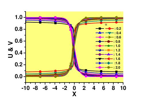
Figure 1: A set of stationary profiles of the two components of the numerically generated DW (domain-wall) solutions of Eq. (4) with $\lambda=0$, $\beta=3$, $k=-1$ and indicated values of the LI (Lévy index) varying from $\alpha=2$ (which corresponds to the normal non-fractional diffraction) up to $\alpha=0.2$.

Furthermore, the numerical solution of the system of linearized equations (LABEL:linearized) for small perturbations produces completely stable spectra of eigenvalues for all stationary DW patterns (not shown here in detail, as they do not exhibit essential peculiarities). The stability of the DWs was also corroborated by direct simulations of the system of underlying equations (1), see a typical examples displayed in Fig. 2 for $\alpha=1$.

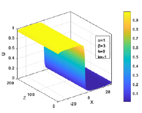
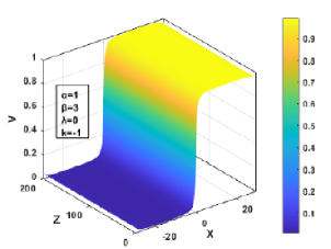
Figure 2: An example of the stable evolution of the two components of the DW [shown in panels (a) and (b)] with $k=-1$, produced by simulations of Eq. (1) with $\alpha=1$, $\beta=3$, and $\lambda=0$. The stability of the DW is corroborated by a purely stable spectrum of eigenvalues produced, for the same DW state, by numerical solution of Eq. (LABEL:linearized) (not shown here).

Similar results, i.e., a family of stable DW solutions, are produced by the numerical analysis of Eqs. (1), (4), and (LABEL:linearized), for values of the XPM coefficient $\beta\neq 3$, as shown by a set of profiles in Fig. 3 for $\alpha=1$ (it is a typical value of the LI corresponding to the fractional diffraction).

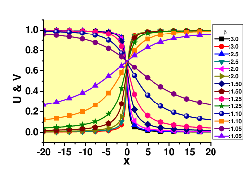
Figure 3: A set of DW solutions with $k=-1$, produced by Eq. (4) with $\lambda=0$, $\alpha=1$ and values of XPM coefficient varying in interval $1.05\leq\beta\leq 3$. All the solutions are stable, according to the calculation of eigenvalues [see Eq. (LABEL:linearized)] and direct simulations of Eq. (1).

The set of DW profiles is displayed in Fig. 3 for $\beta\geq 1.05$, as, for very small values of $\beta-1$, the width of the DW diverges, in accordance with the scaling relation given, for $\lambda=0$, by Eq. (43). For different values of $\alpha$ the DW families are characterized by dependences of their width $L$ on $(\beta-1)$, as shown in the top left panel of Fig. 4. The width was identified, from the numerical solution, as the distance between points where $U(x)$ and $V(x)$ take values $1/2$, i.e., half of the asymptotic values $U(x\rightarrow-\infty)=V(x=+\infty)=1$ for $k=-1$, see Eqs. (12) and (17). In the same figure 4, the numerically found dependences are compared to the analytically predicted asymptotic scaling relations given by Eq. (43). It is seen that the prediction is indeed very close to the numerical results for sufficiently small values of $\left(\beta-1\right)$.

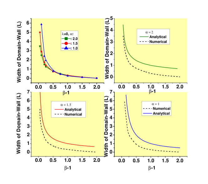
Figure 4: The top left panel: Width $L$ of the DW for $k=-1$, $\lambda=0$, and three different values of the LI, $\alpha=2$ (which corresponds to the normal non-fractional diffraction), $\alpha=1.5$, and $\alpha=1,$ vs. the proximity, $\left(\beta-1\right)$, to the DW’s existence threshold, $\beta=1$. The other panels show the comparison of the respective numerically found curves, $L(\beta-1)$, to the asymptotic analytically predicted scaling relation (43).

IV.2 The system including the linear coupling ($\lambda>0$)

The inclusion of the linear coupling in Eq. (4) neither destroys DW solutions nor destabilizes them, but makes their shapes more complex, even in the case of $\beta=3$, when substitution (33) reduces the system of two equations (4) to the single equation (34). First, Fig. 5(a) demonstrates that the linear coupling with strength $\lambda=0.5$ produces a relatively weak effect on the shape of the DW states if the LI takes values in the interval of $1\leq\alpha\leq 2$. On the other hand, Fig. 5(b) demonstrates a more conspicuous effect of the same linear coupling for smaller values of the LI, viz., in the interval of $0.1\leq\alpha<1$: the corresponding DWs become essentially broader, in comparison to their counterparts found at $\lambda=0$. These results are summarized by Fig. 5(c), where, in a broader spatial domain, it is shown that the DW solutions eventually converge to asymptotic values at $|x|\rightarrow\infty$, which are, according to Eqs. (35) and (33),

$$U_{\pm}=\left(\sqrt{0.725}\pm\sqrt{0.225}\right)/\sqrt{2}\approx\left\{0.94,0.27\right\}$$ (44)

for the case of $k=1$, $\lambda=0.5$, $\beta=3$, although at small values of $\alpha$ the convergence is very slow. These findings are readily explained by the scaling relation (37), which predicts the growth of the DW’s width with the increase of the linear-coupling constant $\lambda$ and decrease of the LI, $\alpha$.

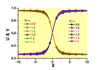
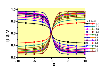
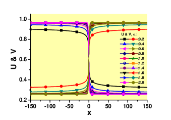
Figure 5: Shapes of stable DW solutions produced by Eqs. (33) and (34) for $\beta=3$, $\lambda=0.5$, $k=1$, and the LI varying in intervals indicated in the panels. (a) Narrow DWs for $1\leq\alpha\leq 2$; (b) broad DWs for $0.1\leq\alpha<1$ [for the comparison’s sake, the DW profile with $\alpha=2$, i.e., in the case of the normal diffraction, is also included in (b)]; (c) both narrow and broad DWs, displayed in a much larger spatial domain for the entire range of the values of the LI, $0.2\leq\alpha\leq 2$.

The effects of the linear coupling on the DW states at $\beta\neq 3$ are qualitatively similar to those displayed in Fig. 5 for $\beta=3$. In all the cases, the DW solutions remain stable if the linear coupling is incorporated. Further, for comparison of the $L(\beta-1)$ dependences which are displayed for $\lambda=0$ in Fig. 4, similar dependences for $\lambda=0.5$ are presented in Fig. 6. In this case, the dependencies end close to $\beta-1=1$, in accordance with Eq. (20), which gives $\left(\beta-1\right)_{\mathrm{immisc}}=1$ for $\lambda=0.5$ and $k=-1$. The fact that all the curves yield the same DWs’ width at $\beta=3$ is explained by the above finding that this value plays a special role, simplifying the DW solutions.

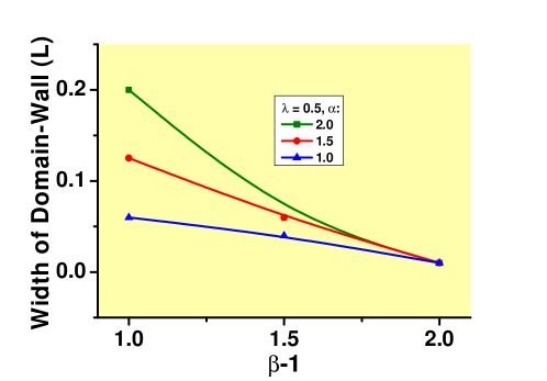
Figure 6: The numerically found dependences of width $L$ of the DW on $\left(\beta-1\right)$ for $k=-1$, $\lambda=0.5$, and three different values of the LI, $\alpha=2$ (which corresponds to the normal non-fractional diffraction), $\alpha=1.5$, and $\alpha=1$.

IV.3 DWs in a system with unequal diffraction coefficients and different values of the Lévy index

A relevant generalization of the system of coupled equations which give rise to DW solutions is one with different diffraction coefficients, $D_{1}\neq D_{2}$, in the two equations, as recently proposed in Ref. [49] (in the case of the normal diffraction). In the optical system, unequal coefficients $D_{1,2}\equiv\cos^{2}\theta_{1,2}$ are determined by different angles $\theta_{1,2}$ between carrier wave vectors of the two components of the light waves and the common propagation direction. The effective diffraction coefficients are also unequal in the BEC model including two heteronuclear components with different atomic masses, $m_{1,2}\sim 1/D_{1,2}$, but in the latter case only the system with $\lambda=0$ is a physically relevant one (two different atomic species cannot transform into each other).

The extension of Eq. (4) with $D_{1}\neq D_{2}$ takes the form of

$$kU+\frac{D_{1}}{2}\left(-\frac{\partial^{2}}{\partial x^{2}}\right)^{\alpha/2}U+(U^{2}+\beta V^{2})U-\lambda V = 0,$$

$$kV+\frac{D_{2}}{2}\left(-\frac{\partial^{2}}{\partial x^{2}}\right)^{\alpha/2}V+(V^{2}+\beta U^{2})V-\lambda U = 0.$$ (45)

The numerical solution of Eq. (45) demonstrates that the asymmetry of the diffraction coefficients makes the shapes of the two components of the DWs mutually asymmetric, but does not destroy them. An example of the so deformed shape of the DWs is displayed in Fig. 7, for both cases of $\lambda=0$ and $\lambda>0$. This solution and all others produced by the asymmetric system remain completely stable, as shown by the solution of the respectively modified Eq. (LABEL:linearized), as well as by direct simulations of the asymmetric version of Eq. (1) (not shown here in detail).

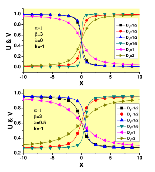
Figure 7: Examples of stable asymmetric DWs with $D_{1}\neq D_{2}$, produced by the numerical solution of Eq. (45) with $\alpha=1$, $\beta=3$, $k=-1,$ and two different values of the linear-coupling constant, $\lambda=0$ and $\lambda=0.5$ in the top and bottom panels. respectively. The two field components, $U$ and $V$, are displayed for three pairs of values $D_{1,2}$, which are indicated, from top to bottom, in the panels.

Furthermore, it is also possible to consider the system with different values of the LI, $\alpha_{1}\neq\alpha_{2}$, in the equations for the two components:

$$kU+\frac{D_{1}}{2}\left(-\frac{\partial^{2}}{\partial x^{2}}\right)^{\alpha_{1}/2}U+(U^{2}+\beta V^{2})U-\lambda V = 0,$$

$$kV+\frac{D_{2}}{2}\left(-\frac{\partial^{2}}{\partial x^{2}}\right)^{\alpha_{1}/2}V+(V^{2}+\beta U^{2})V-\lambda U = 0,$$ (46)

where we set $\alpha_{1}=2$ (non-fractional diffraction) and $\alpha_{2}=1$. Such a system may be realized in terms of BEC, considering immiscible components which represent usual particles ($U$) and those moving by the Lévy flights ($V$). This system also supports stable DW states, as shown in Fig. 8.

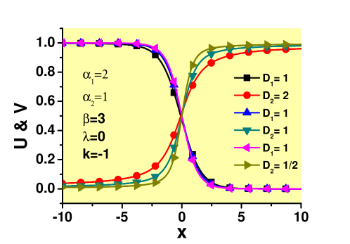
Figure 8: Examples of stable asymmetric DWs with different values of the LI in the two componnts, $\alpha_{1}=2$ and $\alpha_{2}=1$, produced by the numerical solution of Eq. (46) with $\beta=3$, $k=-1,$ and $\lambda=0$. The field components, $U$ and $V$, are displayed for three pairs of values of the diffraction coefficients, $D_{1,2}$, which are indicated, from top to bottom, in the plot.

V Conclusion

The objective of this work is to demonstrate that the variety of states maintained by the interplay of the fractional diffraction and self-defocusing cubic nonlinearity, which may be realized in optics and BEC, can be expanded by predicting stable DWs (domain walls) in the two-component system of immiscible fields. The numerical results clearly demonstrate that, in the entire range of values of the respective LI (Lévy index), $\alpha<2$, that determines the fractional diffraction, and at all values of the relative XPM/SPM coefficient $\beta$, which exceed the immiscibility threshold, given by Eq. (20), the DWs exist and are stable. The same is true for DWs in the system including the linear mixing between the components, in addition to the XPM interaction between them (which makes the immiscibility incomplete). The main characteristic of DW structures is their width. The present analysis demonstrates that the fractional diffraction essentially affects the scaling which determines the dependence of the width on the system’s parameters. Numerical results for the scaling corroborate analytical findings, represented by Eqs. (37), (41), and (43). It is seen that the decrease of $\alpha$ leads to steep increase of the scaling exponents $\sim 1/\alpha$, which is explained by the fact that the fractional diffraction is represented by the nonlocal operator [the Riesz derivative, defined as per Eq. (2)]. It is also demonstrated that the DW solutions are essentially simplified in the special case of $\beta=3$. Currently available techniques should make it possible to create the predicted DWs patterns in the experiment that may be performed for the bimodal light propagation in the temporal domain [75].

As extension of the present analysis, it may be natural to study static and dynamical states built as multi-DW patterns. Another relevant direction is the consideration of two-dimensional settings, such as radial DWs (also in static and dynamical states) between immiscible light waves in bulk waveguides, cf. Refs. [76]-[80].

References

- [1] N. Laskin, Fractional quantum mechanics and Lévy path integrals. Phys. Lett. A 268, 298-305 (2000).
- [2] N. Laskin, Fractional quantum mechanics (World Scientific: Singapore, 2018).
- [3] S. Longhi, Fractional Schrödinger equation in optics. Opt. Lett. 40, 1117-1120 (2015).
- [4] Y. Zhang, X. Liu, M. R. Belić, W. Zhong, Y. Zhang, M. Xiao, Propagation dynamics of a light beam in a fractional Schrödinger equation, Phys. Rev. Lett. 115(18), 180403 (2015).
- [5] B. A. Stickler, Potential condensed-matter realization of space-fractional quantum mechanics: The one-dimensional Lévy crystal. Phys. Rev. E 88, 012120 (2013).
- [6] F. Pinsker, W. Bao, Y. Zhang, H. Ohadi, A. Dreismann, and J. J. Baumberg, Fractional quantum mechanics in polariton condensates with velocity-dependent mass. Phys. Rev. B 92, 195310 (2015).
- [7] Y. Zhang, H. Zhong, M. R. Belić, Y. Zhu, W. Zhong, Y. Zhang, D. N. Christodoulides, M. Xiao, symmetry in a fractional Schrödinger equation, Laser Photonics Rev. 10(3), 526-531 (2016).
- [8] P. Li, J. Li, B. Han, H. Ma, and D. Mihalache, D.: -symmetric optical modes and spontaneous symmetry breaking in the space-fractional Schrödinger equation, Rom. Rep. Phys. 71, 106 (2019).
- [9] L. Zeng, J. Shi, X. Lu, Y. Cai, Q. Zhu, H. Chen, H. Long, and J. Li, Stable and oscillating solitons of -symmetric couplers with gain and loss in fractional dimension. Nonlinear Dyn. 103, 1831-1840 (2021).
- [10] P. Li, B. A. Malomed and D. Mihalache, Symmetry-breaking bifurcations and ghost states in the fractional nonlinear Schrödinger equation with a -symmetric potential, Opt. Lett. 46, 3267-3270 (2021).
- [11] S. He, B. A. Malomed, D. Mihalache, X. Peng, X. Yu, Y. He, and D. Den, Propagation dynamics of abruptly autofocusing circular Airy Gaussian vortex beams in the fractional Schrödinger equation, Chaos, Solitons & Fractals 142, 110470 (2021).
- [12] S. He, B. A. Malomed, D. Mihalache, X. Peng, Y. He, and D. Deng, Propagation dynamics of radially polarized symmetric Airy beams in the fractional Schrödinger equation, Phys. Lett. A 404, 127403 (2021).
- [13] L. Zhang, Z. He, C. Conti, Z. Wang, Y. Hu, D. Lei, Y. Li, and D. Fan, Modulational instability in fractional nonlinear Schrödinger equation, Commun. Nonlin. Sci. Numer. Simulat. 48, 531-540 (2017).
- [14] J. Fujioka, A. Espinosa, and R. F. Rodríguez, Fractional optical solitons, Phys. Lett. A 374, 1126-1134 (2010).
- [15] S. Secchi and M. Squassina, Soliton dynamics for fractional Schrödinger equations, Applicable Analysis, 93, 1702-1729 (2014).
- [16] S. Duo and Y. Zhang, Mass-conservative Fourier spectral methods for solving the fractional nonlinear Schrödinger equation, Computers and Mathematics with Applications 71, 2257-2271 (2016).
- [17] W. P. Zhong, M. R. Belić, B. A. Malomed, Y. Zhang, and T. Huang, Spatiotemporal accessible solitons in fractional dimensions, Phys. Rev. E 94, 012216 (2016).
- [18] W. P. Zhong, M. R. Belić, and Y. Zhang, Accessible solitons of fractional dimension, Ann. Phys. 368, 110-116 (2016).
- [19] Y. Hong and Y. Sire, A new class of traveling solitons for cubic fractional nonlinear Schrödinger equations, Nonlinearity 30, 1262-1286 (2017).
- [20] M. Chen, S. Zeng, D. Lu, W. Hu, and Q. Guo, Optical solitons, self-focusing, and wave collapse in a space-fractional Schrödinger equation with a Kerr-type nonlinearity, Phys. Rev. E 98, 022211 (2018).
- [21] Q. Wang, J. Li, L. Zhang, and W. Xie, Hermite-Gaussian-like soliton in the nonlocal nonlinear fractional Schrödinger equation, EPL 122, 64001 (2018).
- [22] Q. Wang, and Z. Z. Deng, Elliptic Solitons in (1+2)-dimensional anisotropic nonlocal nonlinear fractional Schrödinger equation, IEEE Photonics J. 11, 1-8 (2019).
- [23] C. Huang and L. Dong, Gap solitons in the nonlinear fractional Schrödinger equation with an optical lattice, Opt. Lett. 41, 5636-5639 (2016).
- [24] J. Xiao, Z. Tian, C. Huang, and L. Dong, Surface gap solitons in a nonlinear fractional Schrödinger equation, Opt. Express 26, 2650-2658 (2018).
- [25] L. F. Zhang, X. Zhang, H. Z. Wu, C. X. Li, D. Pierangeli, Y. X. Gao, and D. Y. Fan, Anomalous interaction of Airy beams in the fractional nonlinear Schrödinger equation, Opt. Exp. 27, 27936-27945 (2019).
- [26] L. Dong and Z. Tian, Truncated-Bloch-wave solitons in nonlinear fractional periodic systems, Ann. Phys. 404, 57-64 (2019).
- [27] L. Zeng and J. Zeng, One-dimensional gap solitons in quintic and cubic-quintic fractional nonlinear Schrödinger equations with a periodically modulated linear potential, Nonlinear Dyn. 98, 985-995 (2019).
- [28] P. Li, B. A. Malomed, and D. Mihalache, Vortex solitons in fractional nonlinear Schrödinger equation with the cubic-quintic nonlinearity, Chaos Solitons Fract. 137, 109783 (2020).
- [29] Q. Wang and G. Liang, Vortex and cluster solitons in nonlocal nonlinear fractional Schrödinger equation, J. Optics 22, 055501 (2020)
- [30] L. Zeng and J. Zeng, One-dimensional solitons in fractional Schrödinger equation with a spatially periodical modulated nonlinearity: nonlinear lattice, Opt. Lett. 44, 2661-2664 (2019).
- [31] Y. Qiu, B. A. Malomed, D. Mihalache, X. Zhu, X. Peng, and Y. He, Stabilization of single- and multi-peak solitons in the fractional nonlinear Schrödinger equation with a trapping potential, Chaos Solitons Fract. 140, 110222 (2020).
- [32] P. Li, B. A. Malomed, and D. Mihalache, Metastable soliton necklaces supported by fractional diffraction and competing nonlinearities, Opt. Exp. 28, 34472-33488 (2020).
- [33] L. Zeng, D. Mihalache, B. A. Malomed, X. Lu, Y. Cai, Q. Zhu, and J. Li, Families of fundamental and multipole solitons in a cubic-quintic nonlinear lattice in fractional dimension, Chaos Solitons Fract. 144, 110589 (2021).
- [34] L. Zeng and J. Zeng, Preventing critical collapse of higher-order solitons by tailoring unconventional optical diffraction and nonlinearities, Commun. Phys. 3, 26 (2020).
- [35] M. I. Molina, The fractional discrete nonlinear Schrödinger equation, Phys. Lett. A 384, 126180 (2020).
- [36] L. Zeng, B. A. Malomed, D. Mihalache, Y. Cai, X. Lu, Q. Zhu, and J. Li, Bubbles and W-shaped solitons in Kerr media with fractional diffraction, Nonlinear Dynamics 104, 4253-4264 (2021).
- [37] Li, P., Dai C.: Double Loops and Pitchfork Symmetry Breaking Bifurcations of Optical Solitons in Nonlinear Fractional Schrödinger Equation with Competing Cubic-Quintic Nonlinearities, Ann. Phys. (Berlin) 532, 2000048 (2020).
- [38] P. Li, B. A. Malomed, and D. Mihalache, Symmetry breaking of spatial Kerr solitons in fractional dimension, Chaos Solitons Fract. 132, 109602 (2020).
- [39] P. Li, R. Li, and C. Dai, Existence, symmetry breaking bifurcation and stability of two-dimensional optical solitons supported by fractional diffraction, Opt. Exp. 29, 3193-3210 (2021).
- [40] L. Zeng, and J. Zeng, Fractional quantum couplers, Chaos Solitons Fract, 140, 110271 (2020).
- [41] J. Thirouin, On the growth of Sobolev norms of solutions of the fractional defocusing NLS equation on the circle, Ann. Inst. H. Poincare AN34, 509-531 (2017).
- [42] L. Zeng, Y. Zhu, B. A. Malomed,, D. Mihalache, Q. Wang, H. Long, Y. Cai, X. Lu, and J. Li, Quadratic fractional solitons, Chaos, Solitons & Fractals 154, 111586 (2022).
- [43] Y. Qiu, B. A. Malomed, D. Mihalache, X. Zhu, L. Zhang, and Y. He, Soliton dynamics in a fractional complex Ginzburg-Landau model, Chaos Solitons Fract. 131, 109471 (2020).
- [44] B. A. Malomed, Optical solitons and vortices in fractional media: A mini-review of recent results, Photonics 8, 353 (2021).
- [45] P. Manneville, Y. Pomeau, A grain-boundary in cellular structures near the onset of convection. Phil. Mag. A 48, 607-621 (1983).
- [46] V. Steinberg, G. Ahlers, D. S. Cannell, Pattern formation and wave-number selection by Rayleigh-Bénard convection in a cylindrical container, Physica Scripta 32 (1985) 534-547.
- [47] B. A. Malomed, A. A. Nepomnyashchy, M. I. Tribelsky, Domain boundaries in convection patterns. Phys. Rev. A 42, 7244-7263 (1990).
- [48] M. Haragus, G. Iooss, Bifurcation of symmetric domain walls for the Bénard-Rayleigh convection problem. Arch. Rational Mech. Anal. 239, 733-781 (2021).
- [49] B. A. Malomed, New findings for the old problem: Exact solutions for domain walls in coupled real Ginzburg-Landau equations, Phys. Lett. A 422, 127802 (2022).
- [50] G. S. Rohrer, Grain boundary energy anisotropy: a review, J. Materials Science, 46 (2011) 5881-5895.
- [51] H. Lim, M. G. Lee, R. H. Wagoner, Simulation of polycrystal deformation with grain and grain boundary effects, Int. J. Plasticity 27 (2011) 1328-1354.
- [52] P. Rudolph, Dislocation patterning and bunching in crystals and epitaxial layers - a review, Cryst. Res. Tech. 52 (2017) 1600171.
- [53] U. Atxitia, D. Hinzke, U. Nowak, Fundamentals and applications of the Landau-Lifshitz-Bloch equation, J. Phys. D: Appl. Phys. 50 (2017) 033003.
- [54] E. G. Galkina, B. A. Ivanov. Dynamic solitons in antiferromagnets, Low Temp. Phys. 44 (2018) 618-633.
- [55] W. Yao, B. Wu, Y. Liu, Growth and grain boundaries in 2D materials, ACS Nano 14 (2020) 9320-9346.
- [56] B. A. Malomed, Optical domain walls, Phys. Rev. E, 50 (1994) 1565-1571.
- [57] Y. F. Song, X. J. Shi, C. F. Wu, D. Y. Tang, H. Zhang, Recent progress of study on optical solitons in fiber lasers, Appl. Phys. Rev. 6 (2019) 021313.
- [58] V. P. Mineev, The theory of the solution of two near-ideal Bose gases. Zh. Eksp. Teor. Fiz. 67, 263-272 (1974) [English translation: Sov. Phys. – JETP 40, 132-136 (1974)].
- [59] M. E. Gurtin, D. Polignone, J. Vinals, Two-phase binary fluids and immiscible fluids described by an order parameter, Math. Models & Methods in Appl. Sci. 6, 815-831 (1996).
- [60] M. Trippenbach, K. Góral, K. Rzażewski, B. Malomed, Y. B. Band, Structure of binary Bose-Einstein condensates, J. Phys. B: At. Mol. Opt. Phys. 33, (2000) 4017-4031.
- [61] P. G. Kevrekidis, H. E. Nistazakis, D. J. Frantzeskakis, B. A. Malomed, R. Carretero-González, Families of matter-waves in two-component Bose-Einstein condensates, Eur. Phys. J. D 28 (2004), 181-185.
- [62] V. B. Taranenko, I. Ganne, R. J. Kuszelewicz, and C. O. Weiss, Patterns and localized structures in bistable semiconductor resonators, Phys. Rev. A 61, 063818 (2000).
- [63] G. P. Agrawal, Nonlinear Fiber Optics (Academic Press: San Diego, 1995).
- [64] J. D. Joannopoulos, S. G. Johnson, J. N. Winn, and R. D. Meade, Photonic Crystals: Molding the Flow of Light (Princeton University Press, Princeton, 2008).
- [65] M. Skorobogatiy and J. Yang, Fundamentals of Photonic Crystal Guiding (Cambridge University Press, Cambridge, 2009).
- [66] G. Roati, M. Zaccanti, C. D’Errico, J. Catani, M. Modugno, A. Simoni, M. Inguscio, and G. Modugno, 39K Bose-Einstein Condensate with Tunable Interactions, Phys. Rev. Lett. 99, 010403 (2007).
- [67] R. Grimm, P. Julienne, E. Tiesinga, Feshbach resonances in ultracold gases, Rev. Mod. Phys. 82, 1225-1286 (2010).
- [68] R. J. Ballagh, K. Burnett, and T. F. Scott, Theory of an output coupler for Bose-Einstein condensed atoms, Phys. Rev. Lett. 78, 1608-1611 (1997).
- [69] O. P. Agrawal, Fractional variational calculus in terms of Riesz fractional derivatives, J. Phys. A – Math. Theor. 40, 6287-6303 (2007).
- [70] S. I. Muslih, O. P. Agrawal, and D. Baleanu, A Fractional Schrödinger equation and its solution, Int. J. Theor. Phys. 49, 1746-1752 (2010).
- [71] M. Cai and C. P. Li, On Riesz derivative, Fractional Calculus and applied analysis 22, 287-301 (2019).
- [72] I. M. Merhasin, B. A. Malomed, and R. Driben, Transition to miscibility in a binary Bose-Einstein condensate induced by linear coupling, J. Phys. B: At. Mol. Opt. Phys. 38, 877-892 (2005).
- [73] S. V. Manakov, On the theory of two-dimensional stationary self-focusing of electromagnetic waves, Zh. Eksp. Teor. Fiz. 65, 505-516 (1973) [English translation: Sov. Phys. JETP 38, 248-253 (1974)].
- [74] J. Yang, Nonlinear Waves in Integrable and Nonintegrable Systems (SIAM: Philadelphia, 2010).
- [75] S. Liu, Y. Zhang, B. A. Malomed, and E. Karimi, Experimental realisations of the fractional Schrödinger equation in the temporal domain, arXiv:2208.01128 (2022).
- [76] M. Le Berre, D. Leduc, E. Ressayre, and A. Tallet, Striped and circular domain walls in the DOPO, J. Opt. B: Quant. Semicl. Opt. 1, 153-160 (1999).
- [77] M. Tlidi, P. Mandel, M. Le Berre, E. Ressayre, A. Tallet, and L. Di Menza, Phase-separation dynamics of circular domain walls in the degenerate optical parametric oscillator. Opt. Lett. 25, 487-489 (2000).
- [78] D. Gomila, P. Colet, M. San Miguel, A. J. Scroggie, and G. L. Oppo, Stable droplets and dark-ring cavity solitons in nonlinear optical devices, IEEE J. Quant. Elect. 39, 238-244 (2003).
- [79] N. Dror, B. A. Malomed, and J. Zeng, Domain walls and vortices in linearly coupled systems, Phys. Rev. A 84, 046602 (2011).
- [80] L. D. Bookman and M. A. Hoefer, Perturbation theory for propagating magnetic droplet solitons, Proc. Roy. Soc. A: Math. Phys. Eng. Sci. 471, 20150042 (2015).