aainstitutetext: Department of Physics and Astronomy, University of Manchester, Oxford Road, Manchester M13 9PL, United Kingdom

Quantum entanglement and top spin correlations in SMEFT at higher orders

Claudio Severi a    Eleni Vryonidou
Abstract

We present the first analysis of top spin polarizations, tt¯𝑡¯𝑡t\bar{t} spin correlations, and tt¯𝑡¯𝑡t\bar{t} spin entanglement at the LHC in the context of the Standard Model Effective Field Theory, that goes beyond Leading Order QCD accuracy. The complete set of independent dimension-6 operators entering tt¯𝑡¯𝑡t\bar{t} production is identified, and their effects on all top spin observables are extracted at linear and quadratic order in c/Λ2𝑐superscriptΛ2c/\Lambda^{2}. By comparing results at LO and NLO, we note that the inclusion of higher orders, while not dramatically changing the picture, often amounts to notable numerical differences, that are not fully captured by LO scale variation. We also find that the expected deviations from the SM have an intricate phase space structure, and show up predominantly at large top pTsubscript𝑝𝑇p_{T}. For this reason, we advocate for the measurement of spin observables differentially or doubly-differentially in the tt¯𝑡¯𝑡t\bar{t} phase-space. We show how the inclusion of present and future top spin measurements will improve global fits to top LHC data, by also addressing the issue of flat directions.

1 Introduction

The Standard Model Effective Field Theory (SMEFT) is an extension of the Standard Model (SM), that includes a stack of higher–dimensional operators 𝒪ksubscript𝒪𝑘\mathcal{O}_{k},

SMEFT=SM+d=5kckΛd4𝒪k,subscriptSMEFTsubscriptSMsuperscriptsubscript𝑑5subscript𝑘subscript𝑐𝑘superscriptΛ𝑑4subscript𝒪𝑘\mathcal{L}_{\text{SMEFT}}=\mathcal{L}_{\text{SM}}+\sum_{d=5}^{\infty}\sum_{k}\frac{c_{k}}{\Lambda^{d-4}}\mathcal{O}_{k}, (1.1)

parameterized by a set of Wilson coefficients cksubscript𝑐𝑘c_{k} and a global scale ΛΛ\Lambda. This framework offers the significant advantage that only minimal assumptions are put on the new physics (NP): SMEFTsubscriptSMEFT\mathcal{L}_{\text{SMEFT}} is constructed to be the most general Lagrangian that reproduces the SM at low energy, and is Lorentz and SU(3)C×SU(2)L×U(1)Y𝑆𝑈subscript3C𝑆𝑈subscript2L𝑈subscript1YSU(3)_{\text{C}}\times SU(2)_{\text{L}}\times U(1)_{\text{Y}} gauge invariant. The SMEFT provides a promising framework to identify and parameterize deviations from the SM predictions, and a huge effort is underway to combine a wide range of experimental measurements with theoretical predictions in global fits, aimed at constraining the Wilson coefficients of SMEFT operators. The correlating nature of the SMEFT between different observables, different scales, and sometimes different sectors, mandates the inclusion of the largest possible dataset in the fits. Over the last few years, global combinations of LHC data in the top, Higgs and EW sectors have been achieved Buckley:2015lku ; Aguilar-Saavedra:2018ksv ; Hartland:2019bjb ; Brivio:2019ius ; Ellis:2020unq ; Ethier:2021bye . While there has been enormous progress in the SMEFT interpretation of LHC measurements, several operators exist for which the current sensitivity is still limited. Further, global fits are often plagued by the presence of flat directions in their parameter space. One such example arises in the top sector, where several 2-quark and 4-quark operators can modify top interactions. The sheer number of these operators, and the consequent need to break the degeneracies that arise, demands the consideration of the largest possible set of observables.

We are particularly fortunate, in that respect, that almost 30 years after the discovery of the top quark, the remarkable performance of the LHC has moved the top sector of the SM in the realm of precision measurements. A broad campaign is underway involving the study of processes observed at the LHC for the first time: the production of tops in association with a vector boson, with a Higgs, and the simultaneous production of four tops. At the same time, the luminosity and energy reach of the LHC allows precise differential measurements of the main top production channels, both tt¯𝑡¯𝑡t\bar{t} and and single tops, in several final state configurations.

A particularly interesting class of measurements is those focusing on the top spin. Top spin measurements are experimentally very challenging. The first measurement of top spin, establishing the presence of spin correlation in top pairs, was completed in 2012 ATLAS:2012ao . Subsequent studies at s=7TeV𝑠7TeV\sqrt{s}=7\,\text{TeV} ATLAS:2014aus , 8TeV8TeV8\,\text{TeV} CMS:2015cal ; CMS:2016piu ; ATLAS:2016bac , and 13TeV13TeV13\,\text{TeV} CMS:2019nrx ; ATLAS:2019hau ; ATLAS:2019zrq considered more refined observables, and included several different top decay topologies. However, to this date, only one experimental measurement of the full tt¯𝑡¯𝑡t\bar{t} spin density matrix, that completely characterizes top spin polarization and tt¯𝑡¯𝑡t\bar{t} spin correlations, has been published CMS:2019nrx . Furthermore, all the existing experimental measurements were performed inclusively in the tt¯𝑡¯𝑡t\bar{t} phase space; as we will argue in the following, this is a major limitation, as all top spin degrees of freedom exhibit a complex structure in phase space, that is largely washed out if no binning is applied.

Top spin correlation measurements can also be studied in the framework of pure Quantum Mechanics (QM). As first noted in Afik:2020onf , sufficiently strong top spin correlations can signal the presence of quantum entanglement between top quarks. Entanglement, arguably the most essential and counter-intuitive prediction of QM, has been detected experimentally in a variety of physical systems, but never at the TeV scale. As argued in Afik:2020onf , a simple selection based on the tt¯𝑡¯𝑡t\bar{t} invariant mass will be enough to observe entanglement at the LHC. The structure of spin entanglement in tt¯𝑡¯𝑡t\bar{t} pairs has since been studied multiple times, both in the SM and in the SMEFT Afik:2022kwm ; Aguilar-Saavedra:2022uye ; Aoude:2022imd . When entanglement between two particles is sufficiently strong, measurements can be set up so as to violate Bell Inequalities (BI), the ultimate signal of non-classical behavior. A violation of BIs signals correlations so strong that no classical theory, even with arbitrary and hidden degrees of freedom, can explain. Top spin correlations grow with the transverse momentum of tops so that, at extreme pTsubscript𝑝𝑇p_{T}, BIs are violated at parton level. A first analysis Fabbrichesi:2021npl suggested a violation of BIs may be observed at the LHC. Further studies Severi:2021cnj suggested that the experimental verification of BIs will likely be very challenging, and if no new physics is present to enhance spin correlations, the detection of a violation may just escape the reach of the LHC. The investigation of possible BI measurements with top spin in colliders is ongoing, with progress having been reported recently Aguilar-Saavedra:2022uye . Other collider processes have also been investigated Barr:2021zcp ; Barr:2022wyq ; Aguilar-Saavedra:2022wam ; Aguilar-Saavedra:2022mpg ; Ashby-Pickering:2022umy ; Fabbrichesi:2022ovb .

Standard Model predictions for the observables with which experiments can probe all the tt¯𝑡¯𝑡t\bar{t} spin degrees of freedom are available at NLO QCD + EW Bernreuther:2015yna and NNLO QCD Czakon:2020qbd accuracy. Before this work, SMEFT corrections to these observables were available at LO in QCD and LO in c/Λ2𝑐superscriptΛ2c/\Lambda^{2} Bernreuther:2015yna . Quadratic SMEFT corrections for a selection of dimension-6 operators were computed point-by-point in tt¯𝑡¯𝑡t\bar{t} phase space in Aoude:2022imd , for the two LO QCD channels ggtt¯𝑔𝑔𝑡¯𝑡gg\to t\bar{t} and qq¯tt¯𝑞¯𝑞𝑡¯𝑡q\bar{q}\to t\bar{t}.

In this work we will systematically consider the effect of dimension-six operators on tt¯𝑡¯𝑡t\bar{t} entanglement, top spin polarization and tt¯𝑡¯𝑡t\bar{t} spin correlation observables, at the c/Λ2𝑐superscriptΛ2c/\Lambda^{2} and c2/Λ4superscript𝑐2superscriptΛ4c^{2}/\Lambda^{4} level, while also including higher-order QCD corrections.

This paper is organized as follows. In Section 2 we describe the SMEFT operators that enter tt¯𝑡¯𝑡t\bar{t} production at the LHC. In Section 3 we introduce the relevant top spin observables and show how these can be extracted from collider data. Section 4 describes in detail the numerical computation we carried. Results are presented in Section 5 at the inclusive and differential level. In Section 6 we estimate the improvement to global fits caused by the inclusion of spin observables, once more experimental results will become available in the near future. We conclude in Section 7. Finally Appendices A and B contain additional numerical results and plots.

2 SMEFT operators in top pair production

In this section we present the relevant operators entering top pair production at dimension-6. Within this work, we will assume conservation of baryon number and CP invariance. To keep under control the otherwise unmanageable number of four-quark operators, a flavor assumption must be put in place. Several have been proposed, and are studied in detail in Aguilar-Saavedra:2018ksv . We will assume the flavor symmetry as in Degrande:2020evl :

U(2)Q×U(2)u×U(3)d,𝑈subscript2𝑄𝑈subscript2𝑢𝑈subscript3𝑑U(2)_{Q}\times U(2)_{u}\times U(3)_{d}, (2.1)

that implies new physics couples predominantly to top quarks. This is rooted on the unusually large value of the SM top Yukawa coupling yt0.993subscript𝑦𝑡0.993y_{t}\approx 0.993, signaling a special relationship between the two heaviest SM particles, and hinting at the presence of new physics close to the electroweak scale.

We focus on operators containing at least one top quark field, assuming other operators are well enough constrained from measurements not involving tops. All such operators are considered, in a systematic approach, with the exception of those that enter top production only in virtual corrections, and those only entering in highly suppressed contributions (e.g. bb¯tt¯𝑏¯𝑏𝑡¯𝑡b\bar{b}\to t\bar{t}).

2.1 Two-fermion operators

One can write down three dimension-six operators modifying the top-gluon interaction and thus tt¯𝑡¯𝑡t\bar{t} production. To highlight the chiral properties of the induced tt¯g𝑡¯𝑡𝑔t\bar{t}g vertex these can be written as:

𝒪gtsubscript𝒪𝑔𝑡\displaystyle\mathcal{O}_{gt} =t¯TAγμDνtGμνA,absent¯𝑡subscript𝑇𝐴superscript𝛾𝜇superscript𝐷𝜈𝑡superscriptsubscript𝐺𝜇𝜈𝐴\displaystyle=\overline{t}\,T_{A}\gamma^{\mu}D^{\nu}t\,G_{\mu\nu}^{A}, (2.2)
𝒪gQsubscript𝒪𝑔𝑄\displaystyle\mathcal{O}_{gQ} =Q¯TAγμDνQGμνA,absent¯𝑄subscript𝑇𝐴superscript𝛾𝜇superscript𝐷𝜈𝑄superscriptsubscript𝐺𝜇𝜈𝐴\displaystyle=\overline{Q}T_{A}\gamma^{\mu}D^{\nu}QG_{\mu\nu}^{A}, (2.3)
𝒪tGsubscript𝒪𝑡𝐺\displaystyle\mathcal{O}_{tG} =gSQ¯TAφ~σμνtGμνA=gS𝒬uG,33.absentsubscript𝑔𝑆¯𝑄subscript𝑇𝐴~𝜑superscript𝜎𝜇𝜈𝑡superscriptsubscript𝐺𝜇𝜈𝐴subscript𝑔𝑆subscript𝒬𝑢𝐺33\displaystyle=g_{S}\,\overline{Q}T_{A}\tilde{\varphi}\sigma^{\mu\nu}t\,G_{\mu\nu}^{A}=g_{S}\,\mathcal{Q}_{uG,33}. (2.4)

The second equality is in terms of the Warsaw basis Grzadkowski:2010es . Once the additional symmetry (2.1) and the EOM are enforced, only 𝒪tGsubscript𝒪𝑡𝐺\mathcal{O}_{tG} and 𝒪tGsuperscriptsubscript𝒪𝑡𝐺\mathcal{O}_{tG}^{\dagger} survive, as standard manipulations yield:

𝒪gt+𝒪gtsubscript𝒪𝑔𝑡superscriptsubscript𝒪𝑔𝑡\displaystyle\mathcal{O}_{gt}+\mathcal{O}_{gt}^{\dagger} =gs(four-quarks)absentsubscript𝑔𝑠four-quarks\displaystyle=g_{s}\Big{(}\text{four-quarks}\Big{)} (2.5)
𝒪gQ+𝒪gQsubscript𝒪𝑔𝑄superscriptsubscript𝒪𝑔𝑄\displaystyle\mathcal{O}_{gQ}+\mathcal{O}_{gQ}^{\dagger} =gs(four-quarks)absentsubscript𝑔𝑠four-quarks\displaystyle=g_{s}\Big{(}\text{four-quarks}\Big{)} (2.6)
𝒪gt𝒪gtsubscript𝒪𝑔𝑡superscriptsubscript𝒪𝑔𝑡\displaystyle\mathcal{O}_{gt}-\mathcal{O}_{gt}^{\dagger} =𝒪gQ𝒪gQ=ytgS(𝒪tG𝒪tG)absentsuperscriptsubscript𝒪𝑔𝑄subscript𝒪𝑔𝑄subscript𝑦𝑡subscript𝑔𝑆subscript𝒪𝑡𝐺superscriptsubscript𝒪𝑡𝐺\displaystyle=\mathcal{O}_{gQ}^{\dagger}-\mathcal{O}_{gQ}=\frac{y_{t}}{g_{S}}(\mathcal{O}_{tG}-\mathcal{O}_{tG}^{\dagger}) (2.7)

This shows that 𝒪gtsubscript𝒪𝑔𝑡\mathcal{O}_{gt} and 𝒪gQsubscript𝒪𝑔𝑄\mathcal{O}_{gQ} reduce to four-fermion operators; more specifically, they reduce to operators composed of two light quarks and two tops, that will be considered in the following, and to operators with four top quark fields, that we will neglect due to their large suppression in the process at hand. The only surviving operator, 𝒪tGsubscript𝒪𝑡𝐺\mathcal{O}_{tG}, has the effect of deforming the top quark color charge distribution, producing a chromo-magnetic and chromo-electric dipole moment proportional to (ctG)subscript𝑐𝑡𝐺\Re(c_{tG}) and (ctG)subscript𝑐𝑡𝐺\Im(c_{tG}) respectively.

On top of the two-fermion operators listed above, there are five operators involving two fermion fields and electroweak gauge bosons that are in principle relevant for top physics,

𝒬φu, 33subscript𝒬𝜑𝑢33\displaystyle\mathcal{Q}_{\varphi u,\,33} =i(φDμφ)(t¯γμt),absent𝑖subscriptsuperscript𝐷𝜇superscript𝜑𝜑¯𝑡superscript𝛾𝜇𝑡\displaystyle=i(\varphi^{\dagger}\stackrel{{\scriptstyle\leftrightarrow}}{{D}}_{\mu}\varphi)(\overline{t}\gamma^{\mu}t), (2.8)
𝒬φq, 33(1)superscriptsubscript𝒬𝜑𝑞331\displaystyle\mathcal{Q}_{\varphi q,\,33}^{(1)} =i(φDμφ)(Q¯γμQ),absent𝑖subscriptsuperscript𝐷𝜇superscript𝜑𝜑¯𝑄superscript𝛾𝜇𝑄\displaystyle=i(\varphi^{\dagger}\stackrel{{\scriptstyle\leftrightarrow}}{{D}}_{\mu}\varphi)(\overline{Q}\gamma^{\mu}Q), (2.9)
𝒬φq, 33(3)superscriptsubscript𝒬𝜑𝑞333\displaystyle\mathcal{Q}_{\varphi q,\,33}^{(3)} =i(φDμσIφ)(Q¯γμσIQ),absent𝑖subscriptsuperscript𝐷𝜇superscript𝜑subscript𝜎𝐼𝜑¯𝑄superscript𝛾𝜇superscript𝜎𝐼𝑄\displaystyle=i(\varphi^{\dagger}\stackrel{{\scriptstyle\leftrightarrow}}{{D}}_{\mu}\sigma_{I}\varphi)(\overline{Q}\gamma^{\mu}\sigma^{I}Q), (2.10)
𝒬uB, 33subscript𝒬𝑢𝐵33\displaystyle\mathcal{Q}_{uB,\,33} =(Q¯σμνt)φ~Bμν,absent¯𝑄superscript𝜎𝜇𝜈𝑡~𝜑subscript𝐵𝜇𝜈\displaystyle=(\overline{Q}\sigma^{\mu\nu}t)\tilde{\varphi}B_{\mu\nu}, (2.11)
𝒬uW, 33subscript𝒬𝑢𝑊33\displaystyle\mathcal{Q}_{uW,\,33} =(Q¯σμνσIt)φ~WμνI.absent¯𝑄superscript𝜎𝜇𝜈subscript𝜎𝐼𝑡~𝜑superscriptsubscript𝑊𝜇𝜈𝐼\displaystyle=(\overline{Q}\sigma^{\mu\nu}\sigma_{I}t)\tilde{\varphi}W_{\mu\nu}^{I}. (2.12)

Both at 𝒪(c/Λ2)𝒪𝑐superscriptΛ2\mathcal{O}(c/\Lambda^{2}) and 𝒪(c2/Λ4)𝒪superscript𝑐2superscriptΛ4\mathcal{O}(c^{2}/\Lambda^{4}), these operators only enter electroweak top production, and since this process is heavily suppressed with respect to QCD production, their effect will be neglected. An NLO computation including both QCD and EW corrections would be required to fully take into account these contributions.

We note that 𝒬φq, 33(3)superscriptsubscript𝒬𝜑𝑞333\mathcal{Q}_{\varphi q,\,33}^{(3)} and 𝒬uW, 33subscript𝒬𝑢𝑊33\mathcal{Q}_{uW,\,33} also induce a modified tWb𝑡𝑊𝑏tWb vertex. Since spin measurements involve both the production and the decay of the particle at hand, operators that modify the decay of tops enter our study. In the following we will show that their actual effect on the spin observables we consider is negligible.

2.2 Four-fermion operators

There are seven independent dimension-6 operators mediating tt¯𝑡¯𝑡t\overline{t} production by qq¯𝑞¯𝑞q\overline{q} annihilation that result in a color-octet final state. These operators are constructed with a combination of four quark fields, two light (u,d,c,s𝑢𝑑𝑐𝑠u,d,c,s) and two tops. Following the LHC Top WG notation and convention Aguilar-Saavedra:2018ksv , we express SMEFT operators in a basis that highlights their chiral structure:

𝒪tu8superscriptsubscript𝒪𝑡𝑢8\displaystyle\mathcal{O}_{tu}^{8} =f=12(t¯γμTAt)(u¯fγμTAuf)=f=1216𝒬uu,ff33+12𝒬uu,3ff3,absentsuperscriptsubscriptf12¯𝑡subscript𝛾𝜇superscript𝑇𝐴𝑡subscript¯𝑢fsuperscript𝛾𝜇subscript𝑇𝐴subscript𝑢fsuperscriptsubscriptf1216subscript𝒬𝑢𝑢ff3312subscript𝒬𝑢𝑢3ff3\displaystyle=\textstyle\sum_{\text{f}=1}^{2}(\overline{t}\gamma_{\mu}T^{A}t)(\overline{u}_{\text{f}}\gamma^{\mu}T_{A}u_{\text{f}})=\textstyle\sum_{\text{f}=1}^{2}-\frac{1}{6}\mathcal{Q}_{uu,\text{\text{ff33}}}+\frac{1}{2}\mathcal{Q}_{uu,\text{3ff3}}, (2.13)
𝒪td8superscriptsubscript𝒪𝑡𝑑8\displaystyle\mathcal{O}_{td}^{8} =f=13(t¯γμTAt)(d¯fγμTAdf)=f=13𝒬ud,33ff(8),absentsuperscriptsubscriptf13¯𝑡subscript𝛾𝜇subscript𝑇𝐴𝑡subscript¯𝑑fsuperscript𝛾𝜇superscript𝑇𝐴subscript𝑑fsuperscriptsubscriptf13superscriptsubscript𝒬𝑢𝑑33ff8\displaystyle=\textstyle\sum_{\text{f}=1}^{3}(\overline{t}\gamma_{\mu}T_{A}t)(\overline{d}_{\text{f}}\gamma^{\mu}T^{A}d_{\text{f}})=\textstyle\sum_{\text{f}=1}^{3}\mathcal{Q}_{ud,\text{33ff}}^{(8)}, (2.14)
𝒪tq8superscriptsubscript𝒪𝑡𝑞8\displaystyle\mathcal{O}_{tq}^{8} =f=12(q¯fγμTAqf)(t¯γμTAt)=f=12𝒬qu,ff33(8),absentsuperscriptsubscriptf12subscript¯𝑞fsubscript𝛾𝜇subscript𝑇𝐴subscript𝑞f¯𝑡superscript𝛾𝜇superscript𝑇𝐴𝑡superscriptsubscriptf12superscriptsubscript𝒬𝑞𝑢ff338\displaystyle=\textstyle\sum_{\text{f}=1}^{2}(\overline{q}_{\text{f}}\gamma_{\mu}T_{A}q_{\text{f}})(\overline{t}\gamma^{\mu}T^{A}t)=\textstyle\sum_{\text{f}=1}^{2}\mathcal{Q}_{qu,\text{ff33}}^{(8)}, (2.15)
𝒪Qu8superscriptsubscript𝒪𝑄𝑢8\displaystyle\mathcal{O}_{Qu}^{8} =f=12(Q¯γμTAQ)(u¯fγμTAuf)=f=12𝒬qu,33ff(8),absentsuperscriptsubscriptf12¯𝑄subscript𝛾𝜇subscript𝑇𝐴𝑄subscript¯𝑢fsuperscript𝛾𝜇superscript𝑇𝐴subscript𝑢fsuperscriptsubscriptf12superscriptsubscript𝒬𝑞𝑢33ff8\displaystyle=\textstyle\sum_{\text{f}=1}^{2}(\overline{Q}\gamma_{\mu}T_{A}Q)(\overline{u}_{\text{f}}\gamma^{\mu}T^{A}u_{\text{f}})=\textstyle\sum_{\text{f}=1}^{2}\mathcal{Q}_{qu,\text{33ff}}^{(8)}, (2.16)
𝒪Qd8superscriptsubscript𝒪𝑄𝑑8\displaystyle\mathcal{O}_{Qd}^{8} =f=13(Q¯γμTAQ)(d¯fγμTAdf)=f=13𝒬qd,33ff(8),absentsuperscriptsubscriptf13¯𝑄subscript𝛾𝜇subscript𝑇𝐴𝑄subscript¯𝑑fsuperscript𝛾𝜇superscript𝑇𝐴subscript𝑑fsuperscriptsubscriptf13superscriptsubscript𝒬𝑞𝑑33ff8\displaystyle=\textstyle\sum_{\text{f}=1}^{3}(\overline{Q}\gamma_{\mu}T_{A}Q)(\overline{d}_{\text{f}}\gamma^{\mu}T^{A}d_{\text{f}})=\textstyle\sum_{\text{f}=1}^{3}\mathcal{Q}_{qd,\text{33ff}}^{(8)}, (2.17)
𝒪Qq1,8superscriptsubscript𝒪𝑄𝑞18\displaystyle\mathcal{O}_{Qq}^{1,8} =f=12(Q¯γμTAQ)(q¯fγμTAqf)=f=1214𝒬qq,3ff3(1)16𝒬qq,33ff(1)+14𝒬qq,3ff3(3),absentsuperscriptsubscriptf12¯𝑄subscript𝛾𝜇superscript𝑇𝐴𝑄subscript¯𝑞fsuperscript𝛾𝜇subscript𝑇𝐴subscript𝑞fsuperscriptsubscriptf1214superscriptsubscript𝒬𝑞𝑞3ff3116superscriptsubscript𝒬𝑞𝑞33ff114superscriptsubscript𝒬𝑞𝑞3ff33\displaystyle=\textstyle\sum_{\text{f}=1}^{2}(\overline{Q}\gamma_{\mu}T^{A}Q)(\overline{q}_{\text{f}}\gamma^{\mu}T_{A}q_{\text{f}})=\textstyle\sum_{\text{f}=1}^{2}\frac{1}{4}\mathcal{Q}_{qq,\text{3ff3}}^{(1)}-\frac{1}{6}\mathcal{Q}_{qq,\text{33ff}}^{(1)}+\frac{1}{4}\mathcal{Q}_{qq,\text{3ff3}}^{(3)}, (2.18)
𝒪Qq3,8superscriptsubscript𝒪𝑄𝑞38\displaystyle\mathcal{O}_{Qq}^{3,8} =f=12(Q¯γμTAσIQ)(q¯fγμTAσIqf)=f=1234𝒬qq,3ff3(1)16𝒬qq,33ff(3)14𝒬qq,3ff3(3).absentsuperscriptsubscriptf12¯𝑄subscript𝛾𝜇superscript𝑇𝐴subscript𝜎𝐼𝑄subscript¯𝑞fsuperscript𝛾𝜇subscript𝑇𝐴superscript𝜎𝐼subscript𝑞fsuperscriptsubscriptf1234superscriptsubscript𝒬𝑞𝑞3ff3116superscriptsubscript𝒬𝑞𝑞33ff314superscriptsubscript𝒬𝑞𝑞3ff33\displaystyle=\textstyle\sum_{\text{f}=1}^{2}(\overline{Q}\gamma_{\mu}T^{A}\sigma_{I}Q)(\overline{q}_{\text{f}}\gamma^{\mu}T_{A}\sigma^{I}q_{\text{f}})=\textstyle\sum_{\text{f}=1}^{2}\frac{3}{4}\mathcal{Q}_{qq,\text{3ff3}}^{(1)}-\frac{1}{6}\mathcal{Q}_{qq,\text{33ff}}^{(3)}-\frac{1}{4}\mathcal{Q}_{qq,\text{3ff3}}^{(3)}. (2.19)

The second equality in (2.13) – (2.19) again refers to the expression in terms of the Warsaw basis Grzadkowski:2010es . The operators (2.13) – (2.19) can also be considered in their color-singlet version:

𝒪tu1superscriptsubscript𝒪𝑡𝑢1\displaystyle\mathcal{O}_{tu}^{1} =f=12(t¯γμt)(u¯fγμuf)=f=12𝒬uu,ff33,absentsuperscriptsubscriptf12¯𝑡subscript𝛾𝜇𝑡subscript¯𝑢fsuperscript𝛾𝜇subscript𝑢fsuperscriptsubscriptf12subscript𝒬𝑢𝑢ff33\displaystyle=\textstyle\sum_{\text{f}=1}^{2}(\overline{t}\gamma_{\mu}t)(\overline{u}_{\text{f}}\gamma^{\mu}u_{\text{f}})=\textstyle\sum_{\text{f}=1}^{2}\mathcal{Q}_{uu,\text{ff33}}, (2.20)
𝒪td1superscriptsubscript𝒪𝑡𝑑1\displaystyle\mathcal{O}_{td}^{1} =f=13(t¯γμt)(d¯fγμdf)=f=13𝒬ud,33ff(1),absentsuperscriptsubscriptf13¯𝑡subscript𝛾𝜇𝑡subscript¯𝑑fsuperscript𝛾𝜇subscript𝑑fsuperscriptsubscriptf13superscriptsubscript𝒬𝑢𝑑33ff1\displaystyle=\textstyle\sum_{\text{f}=1}^{3}(\overline{t}\gamma_{\mu}t)(\overline{d}_{\text{f}}\gamma^{\mu}d_{\text{f}})=\textstyle\sum_{\text{f}=1}^{3}\mathcal{Q}_{ud,\text{33ff}}^{(1)}, (2.21)
𝒪tq1superscriptsubscript𝒪𝑡𝑞1\displaystyle\mathcal{O}_{tq}^{1} =f=12(q¯fγμqf)(t¯γμt)=f=12𝒬qu,ff33(1),absentsuperscriptsubscriptf12subscript¯𝑞fsubscript𝛾𝜇subscript𝑞f¯𝑡superscript𝛾𝜇𝑡superscriptsubscriptf12superscriptsubscript𝒬𝑞𝑢ff331\displaystyle=\textstyle\sum_{\text{f}=1}^{2}(\overline{q}_{\text{f}}\gamma_{\mu}q_{\text{f}})(\overline{t}\gamma^{\mu}t)=\textstyle\sum_{\text{f}=1}^{2}\mathcal{Q}_{qu,\text{ff33}}^{(1)}, (2.22)
𝒪Qu1superscriptsubscript𝒪𝑄𝑢1\displaystyle\mathcal{O}_{Qu}^{1} =f=12(Q¯γμQ)(u¯fγμuf)=f=12𝒬qu,33ff(1),absentsuperscriptsubscriptf12¯𝑄subscript𝛾𝜇𝑄subscript¯𝑢fsuperscript𝛾𝜇subscript𝑢fsuperscriptsubscriptf12superscriptsubscript𝒬𝑞𝑢33ff1\displaystyle=\textstyle\sum_{\text{f}=1}^{2}(\overline{Q}\gamma_{\mu}Q)(\overline{u}_{\text{f}}\gamma^{\mu}u_{\text{f}})=\textstyle\sum_{\text{f}=1}^{2}\mathcal{Q}_{qu,\text{33ff}}^{(1)}, (2.23)
𝒪Qd1superscriptsubscript𝒪𝑄𝑑1\displaystyle\mathcal{O}_{Qd}^{1} =f=13(Q¯γμQ)(d¯fγμdf)=f=13𝒬qd,33ff(1),absentsuperscriptsubscriptf13¯𝑄subscript𝛾𝜇𝑄subscript¯𝑑fsuperscript𝛾𝜇subscript𝑑fsuperscriptsubscriptf13superscriptsubscript𝒬𝑞𝑑33ff1\displaystyle=\textstyle\sum_{\text{f}=1}^{3}(\overline{Q}\gamma_{\mu}Q)(\overline{d}_{\text{f}}\gamma^{\mu}d_{\text{f}})=\textstyle\sum_{\text{f}=1}^{3}\mathcal{Q}_{qd,\text{33ff}}^{(1)}, (2.24)
𝒪Qq1,1superscriptsubscript𝒪𝑄𝑞11\displaystyle\mathcal{O}_{Qq}^{1,1} =f=12(Q¯γμQ)(q¯fγμqf)=f=12𝒬qq,33ff(1),absentsuperscriptsubscriptf12¯𝑄subscript𝛾𝜇𝑄subscript¯𝑞fsuperscript𝛾𝜇subscript𝑞fsuperscriptsubscriptf12superscriptsubscript𝒬𝑞𝑞33ff1\displaystyle=\textstyle\sum_{\text{f}=1}^{2}(\overline{Q}\gamma_{\mu}Q)(\overline{q}_{\text{f}}\gamma^{\mu}q_{\text{f}})=\textstyle\sum_{\text{f}=1}^{2}\mathcal{Q}_{qq,\text{33ff}}^{(1)}, (2.25)
𝒪Qq3,1superscriptsubscript𝒪𝑄𝑞31\displaystyle\mathcal{O}_{Qq}^{3,1} =f=12(Q¯γμσIQ)(q¯fγμσIqf)=f=12𝒬qq,ff33(3).absentsuperscriptsubscriptf12¯𝑄subscript𝛾𝜇subscript𝜎𝐼𝑄subscript¯𝑞fsuperscript𝛾𝜇superscript𝜎𝐼subscript𝑞fsuperscriptsubscriptf12superscriptsubscript𝒬𝑞𝑞ff333\displaystyle=\textstyle\sum_{\text{f}=1}^{2}(\overline{Q}\gamma_{\mu}\sigma_{I}Q)(\overline{q}_{\text{f}}\gamma^{\mu}\sigma^{I}q_{\text{f}})=\textstyle\sum_{\text{f}=1}^{2}\mathcal{Q}_{qq,\text{ff33}}^{(3)}. (2.26)

Again the second equality in (2.20) – (2.26) refers to the expression in terms of the Warsaw basis Grzadkowski:2010es . When considering only the leading-order SM QCD amplitudes for the Standard Model, these operators effectively enter top production at the 1/Λ41superscriptΛ41/\Lambda^{4} level, since the 𝒪(1/Λ2)𝒪1superscriptΛ2\mathcal{O}(1/\Lambda^{2}) interference arises only with the suppressed electroweak SM production qq¯Z/γtt¯𝑞¯𝑞𝑍𝛾𝑡¯𝑡q\bar{q}\,\to\,Z/\gamma\,\to\,t\bar{t}, or with QCD production at NLO.

3 Spin of top quarks

Top quark pairs are unique candidates for spin polarization and spin correlation measurements. Top production at hadron colliders involves top quarks with negligible individual spin polarization, but large pair spin correlation with an elaborate phase-space structure. In fact, with appropriate cuts, it has been argued that spin correlations become so strong that quantum entanglement can be detected between top pairs Afik:2022kwm and, in principle, the violation of Bell inequalities can also be observed Fabbrichesi:2021npl ; Severi:2021cnj ; Aguilar-Saavedra:2022uye . Furthermore, the spin de-correlation time from non-perturbative strong effects, of order mtΛQCD2subscript𝑚𝑡subscriptsuperscriptΛ2QCDm_{t}\,\Lambda^{-2}_{\text{\tiny QCD}}, is much larger than the top lifetime, so top quarks decay before their initial spin state is lost in the environment. In fact, since the hadronization timescale, ΛQCD1superscriptsubscriptΛQCD1\Lambda_{\text{\tiny{QCD}}}^{-1}, is also about one order of magnitude larger than the top lifetime, tops behave like free, spinning particles.

The spin state of a tt¯𝑡¯𝑡t\bar{t} pair is described by the density matrix:

ρ=14(𝟙𝟙+i=13Biσi𝟙+i=j3B¯j 1σj+i=13j=13Cijσiσj),𝜌14tensor-product11superscriptsubscript𝑖13tensor-productsubscript𝐵𝑖subscript𝜎𝑖1superscriptsubscript𝑖𝑗3tensor-productsubscript¯𝐵𝑗1subscript𝜎𝑗superscriptsubscript𝑖13superscriptsubscript𝑗13tensor-productsubscript𝐶𝑖𝑗subscript𝜎𝑖subscript𝜎𝑗\rho=\frac{1}{4}\Big{(}\mathbbm{1}\otimes\mathbbm{1}+\sum_{i=1}^{3}B_{i}\,\sigma_{i}\otimes\mathbbm{1}+\sum_{i=j}^{3}\bar{B}_{j}\,\mathbbm{1}\otimes\sigma_{j}+\sum_{i=1}^{3}\sum_{j=1}^{3}C_{ij}\,\sigma_{i}\otimes\sigma_{j}\Big{)}, (3.1)

where the first term in each tensor product refers to the top and the second term to the anti-top. The parameters entering (3.1) have the physical interpretation of being the expectation values of individual spins and spin correlations,

Si=Bi,S¯i=B¯j,SiS¯j=Cij.formulae-sequencedelimited-⟨⟩subscript𝑆𝑖subscript𝐵𝑖formulae-sequencedelimited-⟨⟩subscript¯𝑆𝑖subscript¯𝐵𝑗delimited-⟨⟩subscript𝑆𝑖subscript¯𝑆𝑗subscript𝐶𝑖𝑗\langle S_{i}\rangle=B_{i},\quad\langle\bar{S}_{i}\rangle=\bar{B}_{j},\quad\langle S_{i}\bar{S}_{j}\rangle=C_{ij}. (3.2)

The parameters entering (3.1) have well defined C, P, and CP transformation properties Bernreuther:2015yna , listed in Table 1. In particular, the linear combinations BiB¯isubscript𝐵𝑖subscript¯𝐵𝑖B_{i}-\bar{B}_{i} and CijCjisubscript𝐶𝑖𝑗subscript𝐶𝑗𝑖C_{ij}-C_{ji} are CP violating, and will not be considered further in this work.

Spin analyzing power.


The measurement of the tt¯𝑡¯𝑡t\,\bar{t} spin state may be considered to be very challenging, as measuring a particle’s spin traditionally requires careful measurements of its trajectory in a rapidly changing magnetic field. However, provided that the particle one is interested in decays electroweakly, and that its decay products are fully recovered, the reconstruction of the spin state becomes experimentally possible even in the difficult environment of a hadron collider. In fact, thanks to the fully chiral nature of weak interactions, the momenta of daughters X=b,W,,q,ν𝑋𝑏𝑊𝑞𝜈X=b,W,\ell,q,\nu emerging from the decay of tops are correlated with the spin of the initial top, with the decay width given at LO by:

1ΓdΓdcosθX=1+αXcosθX2,1Γ𝑑Γ𝑑subscript𝜃𝑋1subscript𝛼𝑋subscript𝜃𝑋2\frac{1}{\Gamma}\frac{d\Gamma}{d\cos\theta_{X}}=\frac{1+\alpha_{X}\cos\theta_{X}}{2}\,, (3.3)

where αXsubscript𝛼𝑋\alpha_{X} is a parameter known as spin analyzing power of particle X𝑋X, and θXsubscript𝜃𝑋\theta_{X} is the angle between the original top spin and the direction of the emitted X𝑋X in the top rest frame.

Assuming for concreteness that αX>0subscript𝛼𝑋0\alpha_{X}>0, the direction of flight of particle X𝑋X then follows a cosine distribution around the initial top’s spin, with the most likely trajectory being aligned to the spin itself, and the least likely being opposite to it. As a result of this effect, individual decay products can be considered as proxies for the spin of the corresponding top quarks, and correlations between different decay products as proxies for those between the top quark spins.

At leading order in the SM, the spin analyzing power of prompt W𝑊W bosons and charged leptons emerging from the W𝑊W decay is given by:

αW=mt22mW2mb2(mb2mt2)2+(mb2+mt2)mW22mW4×\displaystyle\alpha_{W}=\frac{m_{t}^{2}-2m_{W}^{2}-m_{b}^{2}}{(m_{b}^{2}-m_{t}^{2})^{2}+(m_{b}^{2}+m_{t}^{2})m_{W}^{2}-2m_{W}^{4}}\ \times
×(mbmtmW)(mb+mtmW)(mbmt+mW)(mb+mt+mW) 0.394,\displaystyle\hskip 14.22636pt\times\sqrt{(m_{b}-m_{t}-m_{W})(m_{b}+m_{t}-m_{W})(m_{b}-m_{t}+m_{W})(m_{b}+m_{t}+m_{W})}\ \approx\ 0.394, (3.4)
α=1.subscript𝛼1\displaystyle\alpha_{\ell}=1. (3.5)

It is curious that the charged lepton has a larger spin-analyzing power than its mother, the W𝑊W boson. This is due to the constructive and destructive interference between amplitudes with intermediate W𝑊W bosons of different helicities; this information is lost when considering the direction of flight of the prompt Wb𝑊𝑏Wb pair.

The presence of new physics in the top electroweak couplings, (2.10) and (2.12), can affect the value of α𝛼\alpha Zhang:2010dr . The effect of 𝒬φq, 33(3)superscriptsubscript𝒬𝜑𝑞333\mathcal{Q}_{\varphi q,\,33}^{(3)} is to rescale the SM value of the tWb𝑡𝑊𝑏tWb vertex, with no effect on angular distributions, and thus on α𝛼\alpha. On the other hand, 𝒬uW, 33subscript𝒬𝑢𝑊33\mathcal{Q}_{uW,\,33} can alter spin analyzing powers. The spin analyzing power of the Wb𝑊𝑏Wb pair is modified at the cuW, 33v2/Λ2subscript𝑐𝑢𝑊33superscript𝑣2superscriptΛ2c_{uW,\,33}v^{2}/\Lambda^{2} level, as expected from dimensional analysis. However, interestingly, when considering the full decay tbν𝑡𝑏subscript𝜈t\to b\,\ell\,\nu_{\ell} the on-shell conditions for final-state leptons remove the linear (and cubic) contribution, and we find:

α(cuW, 33)subscript𝛼subscript𝑐𝑢𝑊33\displaystyle\alpha_{\ell}(c_{uW,\,33}) =1cuW, 332v4Λ44(2mt6+3mt4mW26mt2mW4+mW6+12mt4mW2logmW/mt)(mW2mt2)2(mt2+2mW2),absent1superscriptsubscript𝑐𝑢𝑊332superscript𝑣4superscriptΛ442superscriptsubscript𝑚𝑡63superscriptsubscript𝑚𝑡4superscriptsubscript𝑚𝑊26superscriptsubscript𝑚𝑡2superscriptsubscript𝑚𝑊4superscriptsubscript𝑚𝑊612superscriptsubscript𝑚𝑡4superscriptsubscript𝑚𝑊2subscript𝑚𝑊subscript𝑚𝑡superscriptsuperscriptsubscript𝑚𝑊2superscriptsubscript𝑚𝑡22superscriptsubscript𝑚𝑡22superscriptsubscript𝑚𝑊2\displaystyle=1-\frac{c_{uW,\,33}^{2}v^{4}}{\Lambda^{4}}\frac{4(2m_{t}^{6}+3m_{t}^{4}m_{W}^{2}-6m_{t}^{2}m_{W}^{4}+m_{W}^{6}+12m_{t}^{4}m_{W}^{2}\log m_{W}/m_{t})}{(m_{W}^{2}-m_{t}^{2})^{2}(m_{t}^{2}+2m_{W}^{2})}, (3.6)

up to corrections of order cuW, 334v8/Λ8superscriptsubscript𝑐𝑢𝑊334superscript𝑣8superscriptΛ8c_{uW,\,33}^{4}v^{8}/\Lambda^{8} and ΓW2/mW2superscriptsubscriptΓ𝑊2superscriptsubscript𝑚𝑊2\Gamma_{W}^{2}/m_{W}^{2}. The absence of a linear term in (3.6) is the result of delicate cancellations, resulting from the interplay of the equations of motion of the external fermions and the chiral structure of the interaction induced by 𝒪uW,33subscript𝒪𝑢𝑊33\mathcal{O}_{uW,33}. The cancellation is independent of mWsubscript𝑚𝑊m_{W} and mbsubscript𝑚𝑏m_{b}, while it is spoiled by a finite msubscript𝑚m_{\ell}. This has been noted repeatedly in the literature Grzadkowski:2002gt ; Aguilar-Saavedra:2006qvv , published results are in agreement with our (3.6), when considering the different conventions. This result applies to both the positively and the negatively charged lepton. We note that the small pre-factor makes the 𝒬uW, 33subscript𝒬𝑢𝑊33\mathcal{Q}_{uW,\,33} contribution to the lepton spin analyzing power of order 103superscript10310^{-3} or less, assuming recent bounds for its Wilson coefficient. This suggests the dilepton final state is an exceptionally clean channel to investigate new physics in top production, with little contamination from electroweak effects in the top decay.

Higher order QCD corrections to αWsubscript𝛼𝑊\alpha_{W} and αsubscript𝛼\alpha_{\ell} are known in the SM Czarnecki:1990pe ; Brandenburg:2002xr . NLO effects in the top decay can be reduced to a shift in α𝛼\alpha, that we consider, and to very limited corrections to the functional relation (3.3), that are neglected.

Measurement of the spin state.


The differential cross section for the process pptt¯ab𝑝𝑝𝑡¯𝑡𝑎𝑏pp\to t\bar{t}\to ab, where a𝑎a is a decay product of the top quark and b𝑏b is a decay product of the anti-top quark can be expressed as Bernreuther:2015yna :

1σdσdcosθi=1+αaBicosθi2,1σdσdcosθ¯i=1+αbB¯icosθ¯i2formulae-sequence1𝜎𝑑𝜎𝑑subscript𝜃𝑖1subscript𝛼𝑎subscript𝐵𝑖subscript𝜃𝑖21𝜎𝑑𝜎𝑑subscript¯𝜃𝑖1subscript𝛼𝑏subscript¯𝐵𝑖subscript¯𝜃𝑖2\displaystyle\frac{1}{\sigma}\frac{d\sigma}{d\cos\theta_{i}}=\frac{1+\alpha_{a}B_{i}\cos\theta_{i}}{2},\quad\frac{1}{\sigma}\frac{d\sigma}{d\cos\bar{\theta}_{i}}=\frac{1+\alpha_{b}\bar{B}_{i}\cos\bar{\theta}_{i}}{2} (3.7)
1σdσd(cosθicosθ¯j)=1+Cijαaαbcosθicosθ¯j2log|cosθicosθ¯j|,1𝜎𝑑𝜎𝑑subscript𝜃𝑖subscript¯𝜃𝑗1subscript𝐶𝑖𝑗subscript𝛼𝑎subscript𝛼𝑏subscript𝜃𝑖subscript¯𝜃𝑗2subscript𝜃𝑖subscript¯𝜃𝑗\displaystyle\frac{1}{\sigma}\frac{d\sigma}{d(\cos\theta_{i}\cos\bar{\theta}_{j})}=-\frac{1+C_{ij}\alpha_{a}\alpha_{b}\,\cos\theta_{i}\cos\bar{\theta}_{j}}{2}\log\big{|}\cos\theta_{i}\cos\bar{\theta}_{j}\,\big{|}, (3.8)

where θisubscript𝜃𝑖\theta_{i} is the angle between pasubscript𝑝𝑎\vec{p}_{a} and the i𝑖i-th axis in the top rest frame, and θ¯jsubscript¯𝜃𝑗\bar{\theta}_{j} the angle between pbsubscript𝑝𝑏\vec{p}_{b} and the j𝑗j-th axis in the anti-top rest frame.

A suitable reference frame must be defined in order to evaluate the angles θisubscript𝜃𝑖\theta_{i}, θ¯jsubscript¯𝜃𝑗\bar{\theta}_{j}. An advantageous choice is the helicity basis {k^,r^,n^}^𝑘^𝑟^𝑛\{\hat{k},\hat{r},\hat{n}\}, defined in the tt¯𝑡¯𝑡t\bar{t} pair reference frame as:

k^=top direction,r^=p^k^cosθsinθ,n^=p^×k^sinθformulae-sequence^𝑘top directionformulae-sequence^𝑟^𝑝^𝑘𝜃𝜃^𝑛^𝑝^𝑘𝜃\hat{k}=\text{top direction},\quad\hat{r}=\frac{\hat{p}-\hat{k}\,\cos\theta}{\sin\theta},\quad\hat{n}=\frac{\hat{p}\times\hat{k}}{\sin\theta} (3.9)

where p^^𝑝\hat{p} is the beam axis and θ𝜃\theta is the top/anti-top scattering angle in the tt¯𝑡¯𝑡t\bar{t} center of mass frame. There is a sign ambiguity in choosing the beam direction p^^𝑝\hat{p}; for every event, p^^𝑝\hat{p} is chosen so that:

0θπ2.0𝜃𝜋20\leq\theta\leq\frac{\pi}{2}. (3.10)

The integration of (3.7) and (3.8) gives explicit relations to measure the spin state:

Bi=3αacosθi,B¯i=3αbcosθ¯i,Cij=9αaαbcosθicosθ¯j,formulae-sequencesubscript𝐵𝑖delimited-⟨⟩3subscript𝛼𝑎subscript𝜃𝑖formulae-sequencesubscript¯𝐵𝑖delimited-⟨⟩3subscript𝛼𝑏subscript¯𝜃𝑖subscript𝐶𝑖𝑗delimited-⟨⟩9subscript𝛼𝑎subscript𝛼𝑏subscript𝜃𝑖subscript¯𝜃𝑗B_{i}=\big{\langle}\frac{3}{\alpha_{a}}\cos\theta_{i}\big{\rangle},\quad\bar{B}_{i}=\big{\langle}\frac{3}{\alpha_{b}}\cos\bar{\theta}_{i}\big{\rangle},\quad C_{ij}=\big{\langle}\frac{9}{\alpha_{a}\alpha_{b}}\cos\theta_{i}\cos\bar{\theta}_{j}\big{\rangle}, (3.11)

where angle brackets denote the expectation value:

S=s=s||2𝑑Π||2𝑑ΠσSσ.𝑆delimited-⟨⟩𝑠𝑠superscript2differential-dΠsuperscript2differential-dΠsubscript𝜎𝑆𝜎S=\langle s\rangle=\frac{\int s\,|\mathcal{M}|^{2}\,d\Pi}{\int|\mathcal{M}|^{2}\,d\Pi}\equiv\frac{\sigma_{S}}{\sigma}. (3.12)

The above relations show that an arbitrary spin observable S𝑆S can be extracted as a ratio of two cross sections: the numerator σSsubscript𝜎𝑆\sigma_{S} is the phase-space integral of s𝑠s, some dimensionless combination of angles and spin analysing powers, weighted with the matrix element squared, and the denominator is the total cross section. Further, as the various examples proposed in Ref. Aguilar-Saavedra:2022uye show, it is possible to construct combination of angles s𝑠s so that sdelimited-⟨⟩𝑠\langle s\rangle is directly sensitive to several quantities of interest, e.g. Bi±Bjplus-or-minussubscript𝐵𝑖subscript𝐵𝑗B_{i}\pm B_{j}, Cij±Cjiplus-or-minussubscript𝐶𝑖𝑗subscript𝐶𝑗𝑖C_{ij}\pm C_{ji}, Cii+|Cjj+Ckk|subscript𝐶𝑖𝑖subscript𝐶𝑗𝑗subscript𝐶𝑘𝑘C_{ii}+|C_{jj}+C_{kk}|.

The observables used in this work, that are those commonly considered in spin measurements, are listed in Tab. 1, together with their transformation properties under P and CP. Standard Model predictions for the spin observables of Tab. 1 for tt¯𝑡¯𝑡t\bar{t} pairs produced at the LHC are already available at NNLO QCD Czakon:2020qbd and NLO QCD + EW Bernreuther:2015yna .

CP even CP odd
Bk+B¯ksubscript𝐵𝑘subscript¯𝐵𝑘B_{k}+\overline{B}_{k} P-odd BkB¯ksubscript𝐵𝑘subscript¯𝐵𝑘B_{k}-\overline{B}_{k} P-odd
Br+B¯rsubscript𝐵𝑟subscript¯𝐵𝑟B_{r}+\overline{B}_{r} P-odd BrB¯rsubscript𝐵𝑟subscript¯𝐵𝑟B_{r}-\overline{B}_{r} P-odd
Bn+B¯nsubscript𝐵𝑛subscript¯𝐵𝑛B_{n}+\overline{B}_{n} P-even BnB¯nsubscript𝐵𝑛subscript¯𝐵𝑛B_{n}-\overline{B}_{n} P-even
Ckksubscript𝐶𝑘𝑘C_{kk} P-even
Crrsubscript𝐶𝑟𝑟C_{rr} P-even
Cnnsubscript𝐶𝑛𝑛C_{nn} P-even
Ckr+Crksubscript𝐶𝑘𝑟subscript𝐶𝑟𝑘C_{kr}+C_{rk} P-even CkrCrksubscript𝐶𝑘𝑟subscript𝐶𝑟𝑘C_{kr}-C_{rk} P-even
Ckn+Crnsubscript𝐶𝑘𝑛subscript𝐶𝑟𝑛C_{kn}+C_{rn} P-odd CknCrnsubscript𝐶𝑘𝑛subscript𝐶𝑟𝑛C_{kn}-C_{rn} P-odd
Crn+Crnsubscript𝐶𝑟𝑛subscript𝐶𝑟𝑛C_{rn}+C_{rn} P-odd CrnCrnsubscript𝐶𝑟𝑛subscript𝐶𝑟𝑛C_{rn}-C_{rn} P-odd
Table 1: Top spin polarization and tt¯𝑡¯𝑡t\bar{t} spin correlation observables with their C and CP transformation properties. The CP-even observables are those considered in this work, the CP-even observables are needed in principle for a full reconstruction of the density matrix ρ𝜌\rho, but they are not considered here.

In the SMEFT, allowing at most one NP insertion in each Feynman diagram, cross sections are quadratic functions of the Wilson coefficients so that:

S=σS(0)+c^σS(1)+c^2σS(2)σ(0)+c^σ(1)+c^2σ(2),c^cΛ2/(1TeV)2.formulae-sequence𝑆superscriptsubscript𝜎𝑆0^𝑐superscriptsubscript𝜎𝑆1superscript^𝑐2superscriptsubscript𝜎𝑆2superscript𝜎0^𝑐superscript𝜎1superscript^𝑐2superscript𝜎2^𝑐𝑐superscriptΛ2superscript1TeV2S=\frac{\sigma_{S}^{(0)}+\hat{c}\,\sigma_{S}^{(1)}+\hat{c}^{2}\,\sigma_{S}^{(2)}}{\sigma^{(0)}+\hat{c}\,\sigma^{(1)}+\hat{c}^{2}\,\sigma^{(2)}},\qquad\hat{c}\equiv\frac{c}{\Lambda^{2}\,/\,(1\,\text{TeV})^{2}}. (3.13)

The expression in (3.13) can be series expanded around the SM value,

S=σS(0)σ0+c^σS(1)σ(0)σS(0)σ(1)(σ0)2+,𝑆superscriptsubscript𝜎𝑆0superscript𝜎0^𝑐superscriptsubscript𝜎𝑆1superscript𝜎0superscriptsubscript𝜎𝑆0superscript𝜎1superscriptsuperscript𝜎02S=\frac{\sigma_{S}^{(0)}}{\sigma^{0}}+\hat{c}\>\frac{\sigma_{S}^{(1)}\,\sigma^{(0)}-\sigma_{S}^{(0)}\,\sigma^{(1)}}{(\sigma^{0})^{2}}+\cdots, (3.14)

so that a linear, quadratic, and so on, shift can be extracted. However, to maintain generality, we extract the six cross sections in (3.13) separately, so that the full dependence of S𝑆S on c𝑐c can be evaluated.

Accurate SM predictions can be implemented in several ways, such as:

  • the SM cross sections σS(0)superscriptsubscript𝜎𝑆0\sigma_{S}^{(0)} and σ(0)superscript𝜎0\sigma^{(0)} in (3.13) are replaced by their most accurate values, EFT terms are not modified, and then the ratio S𝑆S is taken;

  • numerator and denominator of (3.13) are globally rescaled by the SM K-factors KS=σS,accurate(0)/σS(0)subscript𝐾𝑆superscriptsubscript𝜎𝑆accurate0superscriptsubscript𝜎𝑆0K_{S}=\sigma_{S,\text{accurate}}^{(0)}/\sigma_{S}^{(0)} and K=σaccurate(0)/σ(0)𝐾superscriptsubscript𝜎accurate0superscript𝜎0K=\sigma_{\text{accurate}}^{(0)}/\sigma^{(0)}, then and the ratio S𝑆S is taken;

  • the ratio (3.13) is series expanded, the first term σS(0)/σ(0)superscriptsubscript𝜎𝑆0superscript𝜎0\sigma_{S}^{(0)}/\sigma^{(0)} is replaced with the accurate value, other terms in the series are not modified – even if they contain σS(0)superscriptsubscript𝜎𝑆0\sigma_{S}^{(0)} or σ(0)superscript𝜎0\sigma^{(0)}.

It is not clear which one, if any, of the prescriptions outlined above entails the best physical meaning, and the spread in results obtained by implementing accurate SM predictions in different ways may be considered to be a theoretical uncertainty. In this work we will report all six cross sections that enter (3.13), leaving the possibility open for arbitrary implementations of accurate SM calculations.

Quantum entanglement.


As discussed in the introduction, and in more detail in Refs. Afik:2020onf ; Severi:2021cnj ; Aoude:2022imd ; Afik:2022kwm , top spin correlations can signal the presence of quantum entanglement between tops. A calculation shows that, in the case of tt¯𝑡¯𝑡t\bar{t}, entanglement is signaled by the condition:

Δ=|Ckk+Crr|Cnn1>0.Δsubscript𝐶𝑘𝑘subscript𝐶𝑟𝑟subscript𝐶𝑛𝑛10\Delta=|C_{kk}+C_{rr}|-C_{nn}-1>0. (3.15)

Inequality (3.15) is general, and independent of the possible presence of new physics. We also note that the concurrence of the tt¯𝑡¯𝑡t\bar{t} spin quantum state (3.1) is given by:

𝒞[ρ]={Δ/2,Δ>00Δ0𝒞delimited-[]𝜌casesΔ2Δ00Δ0\mathcal{C}[\rho]=\begin{dcases}\Delta/2,&\Delta>0\\ 0&\Delta\leq 0\end{dcases} (3.16)

The absolute value in the definition of ΔΔ\Delta is non-trivial, as, already in the SM, at tt¯𝑡¯𝑡t\bar{t} threshold Ckk+Crr<0subscript𝐶𝑘𝑘subscript𝐶𝑟𝑟0C_{kk}+C_{rr}<0, so Δ=TrC1ΔTr𝐶1\Delta=-\text{Tr}\,C-1, while at large top pTsubscript𝑝𝑇p_{T}, Ckk+Crr>0subscript𝐶𝑘𝑘subscript𝐶𝑟𝑟0C_{kk}+C_{rr}>0, so ΔΔ\Delta becomes Ckk+CrrCnn1subscript𝐶𝑘𝑘subscript𝐶𝑟𝑟subscript𝐶𝑛𝑛1C_{kk}+C_{rr}-C_{nn}-1. The use of TrCTr𝐶\text{Tr}\,C to detect entanglement at tt¯𝑡¯𝑡t\bar{t} threshold has been the topic of extended studies Afik:2020onf ; Afik:2022kwm ; in fact, as shown in Ref. Aguilar-Saavedra:2022uye , ΔΔ\Delta can be measured directly using dedicated angular observables, regardless of the sign of the absolute value. To appreciate directly the effect of SMEFT operators on the amount of spin entanglement, in the following we will consider:

Δ±=±(Ckk+Crr)Cnn1=±(σCkk+σCrr)σCnnσσsuperscriptΔplus-or-minusplus-or-minussubscript𝐶𝑘𝑘subscript𝐶𝑟𝑟subscript𝐶𝑛𝑛1plus-or-minussubscript𝜎subscript𝐶𝑘𝑘subscript𝜎subscript𝐶𝑟𝑟subscript𝜎subscript𝐶𝑛𝑛𝜎𝜎\Delta^{\pm}=\pm(C_{kk}+C_{rr})-C_{nn}-1=\frac{\pm(\sigma_{C_{kk}}+\sigma_{C_{rr}})-\sigma_{C_{nn}}-\sigma}{\sigma} (3.17)

as additional observables, as an extension to those appearing in (3.1). We note that ΔsuperscriptΔ\Delta^{-} is a well known top spin observable, usually called D(Δ+1)/3𝐷superscriptΔ13D\equiv(\Delta^{-}+1)/3.

4 Computation Setup

Since the reconstruction of a spin quantum state requires the analysis of decay products, the analysis of top spin polarization and correlations at NLO would require the generation of events of the form:

ppbb¯+νν¯𝑝𝑝𝑏¯𝑏superscriptsuperscript𝜈¯𝜈p\ p\to b\,\bar{b}\,\ell^{+}\,\ell^{-}\,\nu\,\bar{\nu} (4.1)

at order 𝒪(αs3αEW4)𝒪superscriptsubscript𝛼s3superscriptsubscript𝛼EW4\mathcal{O}(\alpha_{\text{s}}^{3}\,\alpha_{\text{EW}}^{4}). This would fully include virtual corrections, and all off-shell effects for both tops and W𝑊W bosons. This computation is extremely challenging, and as of now can only be handled by purpose-made tools, e.g. Campbell:2012uf ; Campbell:2014kua , that lack the versatility needed to include arbitrary SMEFT operators in the matrix element.

A useful proxy for the full NLO computation could be given by the process:

ppW+Wbb¯𝑝𝑝superscript𝑊superscript𝑊𝑏¯𝑏p\ p\to W^{+}\,W^{-}\,b\,\bar{b} (4.2)

at order 𝒪(αs3αEW2)𝒪superscriptsubscript𝛼s3superscriptsubscript𝛼EW2\mathcal{O}(\alpha_{\text{s}}^{3}\,\alpha_{\text{EW}}^{2}), since the prompt Wb𝑊𝑏W\,b pair emitted by the electroweak decay of tops also has spin analyzing power. For such a computation, suitable phase-space cuts help isolate the doubly resonant contribution pptt¯W+Wbb¯𝑝𝑝𝑡¯𝑡superscript𝑊superscript𝑊𝑏¯𝑏p\ p\to t\,\bar{t}\to W^{+}\,W^{-}\,b\,\bar{b}. Generally speaking, one should cluster parton-level QCD radiation in jets, impose a selection of standard jet cuts, and ask that the invariant mass of the two W𝑊W + b𝑏b-jet pairs is close to mtsubscript𝑚𝑡m_{t}. The full SM amplitude for (4.2) has been evaluated at NLO in Denner:2010jp ; Bevilacqua:2010qb , but the significant complexity of SMEFT amplitudes prevented us from extracting precise enough results for this process.

To obtain our results we combine a NLO fixed-order calculation for the process pptt¯𝑝𝑝𝑡¯𝑡p\ p\to t\,\bar{t} and the modeling of the electroweak decays tb+ν𝑡𝑏superscript𝜈t\to b\,\ell^{+}\,\nu and t¯b¯ν¯¯𝑡¯𝑏superscript¯𝜈\bar{t}\to\bar{b}\,\ell^{-}\,\bar{\nu} with MadSpin Artoisenet:2012st . This yields predictions whose accuracy is summarized in Table 2. Accuracy is NLO QCD, up to virtual corrections to the spin state, that can not be handled by MadSpin. However, as the kinematic state is constructed before the spin state, and the top quarks’ momentum is correlated with their spin111See for instance the argument given in Severi:2021cnj for top pairs emitted at large pTsubscript𝑝𝑇p_{T}., the full-NLO accuracy of the tt¯𝑡¯𝑡t\bar{t} kinematics improves the partial-NLO accuracy of the spin state. It is also true that in the SM virtual corrections to the tt¯𝑡¯𝑡t\bar{t} spin state amount to a percent level shift for most of the observables we consider Bernreuther:2015yna ; Frederix:2021zsh . The only exception is Crrsubscript𝐶𝑟𝑟C_{rr}, for which, given its small value in the SM, the relative correction is  25%similar-toabsentpercent25\sim\,25\%. We thus consider it reasonable to assume that the impact of virtual corrections remains under control also in the SMEFT.

   LO QCD NLO QCD
Real emission Virtual corrections
tt¯𝑡¯𝑡t\,\bar{t} kinematics
tt¯𝑡¯𝑡t\,\bar{t} spin state Approximate
Table 2: Accuracy of the computation resulting from Madgraph5_aMC@NLO and MadSpin.

Hard events featuring a top pair production are generated with Madgraph5_aMC@NLO v3.4.0 at fixed-order NLO QCD accuracy, 𝒪(αs3αEW0)𝒪superscriptsubscript𝛼𝑠3superscriptsubscript𝛼EW0\mathcal{O}(\alpha_{s}^{3}\alpha_{\text{EW}}^{0}). Electroweak corrections, known to amount to a percent-level correction to the total cross section Bernreuther:2006vg , and to very small shifts in the spin observables Bernreuther:2015yna , are not considered. The hadronic center of mass energy is set to s=13.0𝑠13.0\sqrt{s}=13.0 TeV, corresponding to the second run of the LHC. We use the NNPDF3.1 parton distribution function NNPDF:2017mvq at NLO QCD with αs(mZ)=0.118subscript𝛼𝑠subscript𝑚𝑍0.118\alpha_{s}(m_{Z})=0.118. The dataset used to extract this PDF does not include any top spin data. The SM renormalization and factorization scales μRsubscript𝜇R\mu_{\text{R}} and μFsubscript𝜇F\mu_{\text{F}} are set on an event-by-event basis to one fourth of the total transverse energy HTsubscript𝐻𝑇H_{T} of the process, and the SMEFT renormalization scale μEFTsubscript𝜇EFT\mu_{\text{EFT}} is set to the top mass. Events are generated within the SMEFT@NLO model Degrande:2020evl , whose flavor symmetry is (2.1). Note that the flavor symmetry implies that light SM particles, including the b𝑏b quark, are massless, and the CKM matrix is the identity. Other SM input parameters are set to their current experimental values. The SMEFT@NLO model is restricted to only contain the operators of interest, 𝒪tGsubscript𝒪𝑡𝐺\mathcal{O}_{tG} and the four-quark operators (2.13) – (2.19) and (2.20) – (2.26), one at a time. Top quarks are kept on shell.

The leptonic decay of top quarks tb+ν𝑡𝑏superscript𝜈t\to b\,\ell^{+}\,\nu, t¯b¯ν¯¯𝑡¯𝑏superscript¯𝜈\bar{t}\to\bar{b}\,\ell^{-}\,\bar{\nu} is modeled by MadSpin Artoisenet:2012st , adapted to handle fixed-order calculations with minor improvements to the technique described in Frederix:2021zsh . Spin observables are extracted at parton level using charged leptons emerging from the electroweak decay, integrating the expressions that enter in the numerator and denominator of (3.12) separately. The individual contributions entering (3.13) are then extracted by varying the Wilson coefficients and fitting a quadratic dependence.

The sources of theoretical uncertainty we consider are MC statistical uncertainty and scale variation. Statistical uncertainty is estimated with standard procedures, scale variation is evaluated from the envelope of the nine points μR=(HT/8,HT/4,HT/2)subscript𝜇𝑅subscript𝐻𝑇8subscript𝐻𝑇4subscript𝐻𝑇2\mu_{R}=(H_{T}/8,\,H_{T}/4,\,H_{T}/2), μf=(HT/8,HT/4,HT/2)subscript𝜇fsubscript𝐻𝑇8subscript𝐻𝑇4subscript𝐻𝑇2\mu_{\text{f}}=(H_{T}/8,\,H_{T}/4,\,H_{T}/2), μEFT=(mt)subscript𝜇EFTsubscript𝑚𝑡\mu_{\text{EFT}}=(m_{t}).

Validations.


Before moving to NLO accuracy, we validate our setup at LO. We compare the SM tt¯𝑡¯𝑡t\bar{t} spin density matrix we obtain with MadSpin with the one obtained from the benchmark process (4.1), that at LO is feasible. In addition, we compare results with and without the narrow width approximation for tops and W bosons. All our checks show deviations at the 103superscript10310^{-3} level, well below current (and presumably future) experimental accuracy, and other sources of theoretical uncertainty. The SMEFT effects on the tt¯𝑡¯𝑡t\bar{t} spin density matrix of the two-fermion operator (2.4) and of the four-fermion color-octet operators (2.13) - (2.19) were computed at LO QCD and LO in c/Λ2𝑐superscriptΛ2c/\Lambda^{2} in Bernreuther:2015yna . After accounting for the different choice of operators, we are able to replicate the results found in Bernreuther:2015yna , up to relative deviations of order 10%percent1010\%. We note that computational setup in Bernreuther:2015yna features a different PDF, different choices of factorization and renormalization scales, and different numerical input parameters with respect to the one presented in this work, so perfect numerical agreement is not expected. However, the pattern of deviations from the SM, and their relative size, is found to be in good agreement. To further check compatibility, we reproduced the exact setup of Bernreuther:2015yna in a LO run with the operator 𝒪tGsubscript𝒪𝑡𝐺\mathcal{O}_{tG}, and obtained agreement at the 104superscript10410^{-4} level.

5 Results and discussion

Our numerical integration is carried:

  • Inclusive in tt¯𝑡¯𝑡t\bar{t} phase space.

  • Binned in tt¯𝑡¯𝑡t\bar{t} phase space, with a 3×3333\times 3 binning in the tt¯𝑡¯𝑡t\bar{t} invariant mass mtt¯subscript𝑚𝑡¯𝑡m_{t\bar{t}} and the center of mass scattering angle θ𝜃\theta. This binning will be updated to match the actual resolution of experimental measurements, once available.

In any case, we do not impose any cuts or detector acceptance effects on the final state b+νb¯ν¯𝑏superscript𝜈¯𝑏superscript¯𝜈b\,\ell^{+}\,\nu\,\bar{b}\,\ell^{-}\,\bar{\nu}. The plots in this Section collect results for the fifteen SMEFT operators inclusive in phase space, and for selected operators binned in phase space, using the sample mtt¯cosθsubscript𝑚𝑡¯𝑡𝜃m_{t\bar{t}}\,-\,\cos\theta binning we considered. Appendix A contains tables with all cross-sections needed to replicate our plots inclusive in phase space. Plots with binned results for operators not included in this Section are in Appendix B.

To highlight the improvement offered by our NLO calculation over the LO, in Appendix A the cross-sections we obtained are provided separately at LO and NLO accuracy. The large K𝐾K-factor of the total cross-section σ𝜎\sigma makes the numerical comparison between LO and NLO not obvious. However, after taking the appropriate ratios, we find that, frequently, NLO results are appreciably different from LO ones. As expected, NLO results also tend to show a smaller scale variation.

5.1 Results inclusive in tt¯𝑡¯𝑡t\bar{t} phase space

The following Figures 1 - 3 show the change with respect to the SM value, defined as:

ΔS=σS(0)+c^σS(1)+c^2σS(2)σ(0)+c^σ(1)+c^2σ(2)σS(0)σ(0),Δ𝑆superscriptsubscript𝜎𝑆0^𝑐superscriptsubscript𝜎𝑆1superscript^𝑐2superscriptsubscript𝜎𝑆2superscript𝜎0^𝑐superscript𝜎1superscript^𝑐2superscript𝜎2superscriptsubscript𝜎𝑆0superscript𝜎0\Delta S=\frac{\sigma_{S}^{(0)}+\hat{c}\,\sigma_{S}^{(1)}+\hat{c}^{2}\,\sigma_{S}^{(2)}}{\sigma^{(0)}+\hat{c}\,\sigma^{(1)}+\hat{c}^{2}\,\sigma^{(2)}}-\frac{\sigma_{S}^{(0)}}{\sigma^{(0)}}, (5.1)

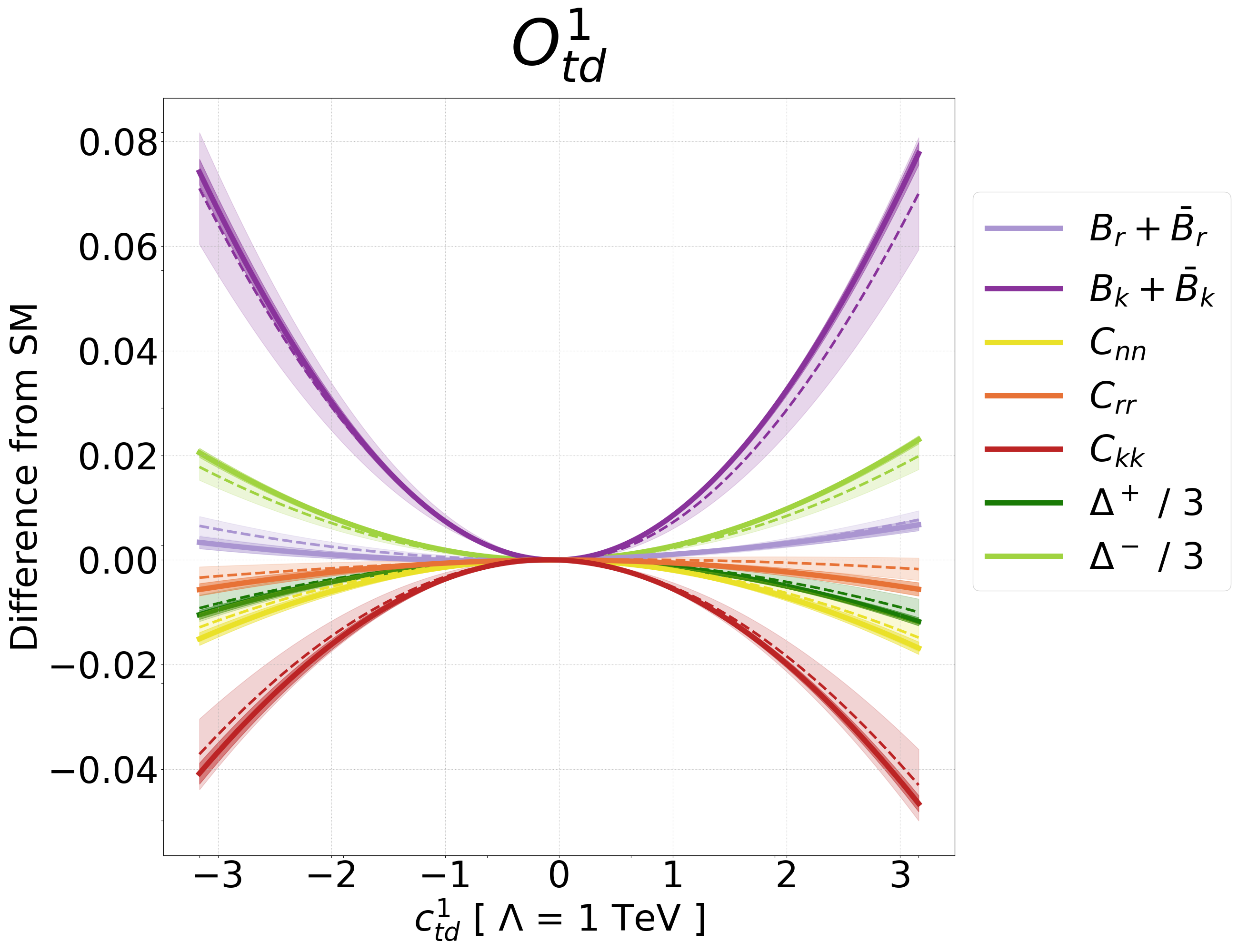
for the top spin polarizations Bi+B¯isubscript𝐵𝑖subscript¯𝐵𝑖B_{i}+\bar{B}_{i}, the tt¯𝑡¯𝑡t\bar{t} spin correlations Ciisubscript𝐶𝑖𝑖C_{ii} and Cij+Cjisubscript𝐶𝑖𝑗subscript𝐶𝑗𝑖C_{ij}+C_{ji}, and the entanglement markers Δ±superscriptΔplus-or-minus\Delta^{\pm}, as a function of the Wilson coefficient of the operators we consider, inclusive in tt¯𝑡¯𝑡t\bar{t} phase space. Similarly to (3.13), in (5.1) we defined c^c(1TeV)2/Λ2^𝑐𝑐superscript1TeV2superscriptΛ2\hat{c}\equiv c\ (1\,\text{TeV})^{2}/\Lambda^{2}, which is equivalent numerically to setting Λ=1TeVΛ1TeV\Lambda=1\,\text{TeV}. For the purposes of plotting results, we employ our own NLO QCD SM predictions σS(0)superscriptsubscript𝜎𝑆0\sigma_{S}^{(0)} and σ(0)superscript𝜎0\sigma^{(0)} in (5.1). Accurate SM predictions, as discussed above, may also be used in (5.1). However, as the leading SM contribution is subtracted, the actual numerical difference is negligible in the range we consider. While, as we will see in the following, an inclusive measurement hides most of the physical features present, we can still highlight several interesting points, presented in the rest of this Section.

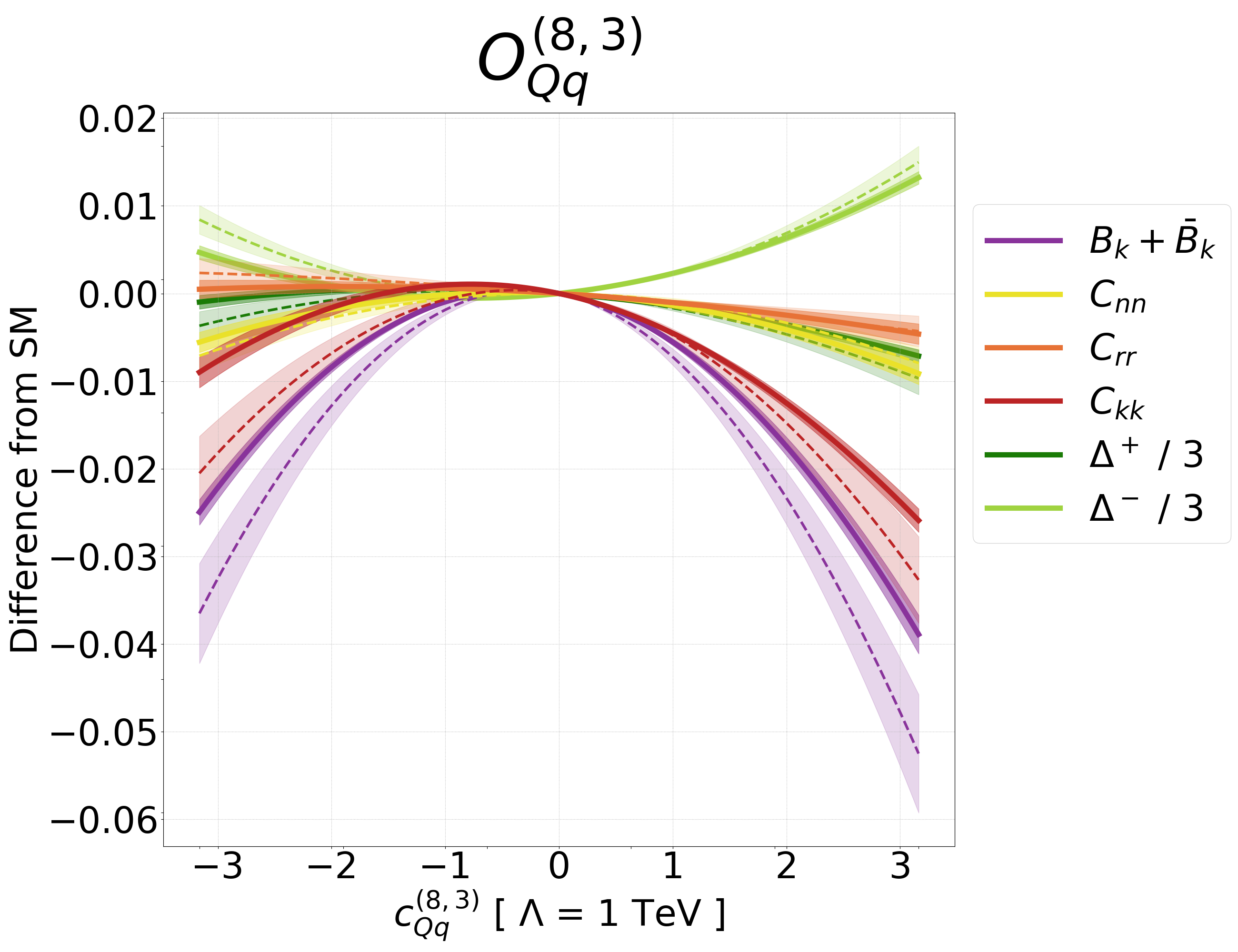
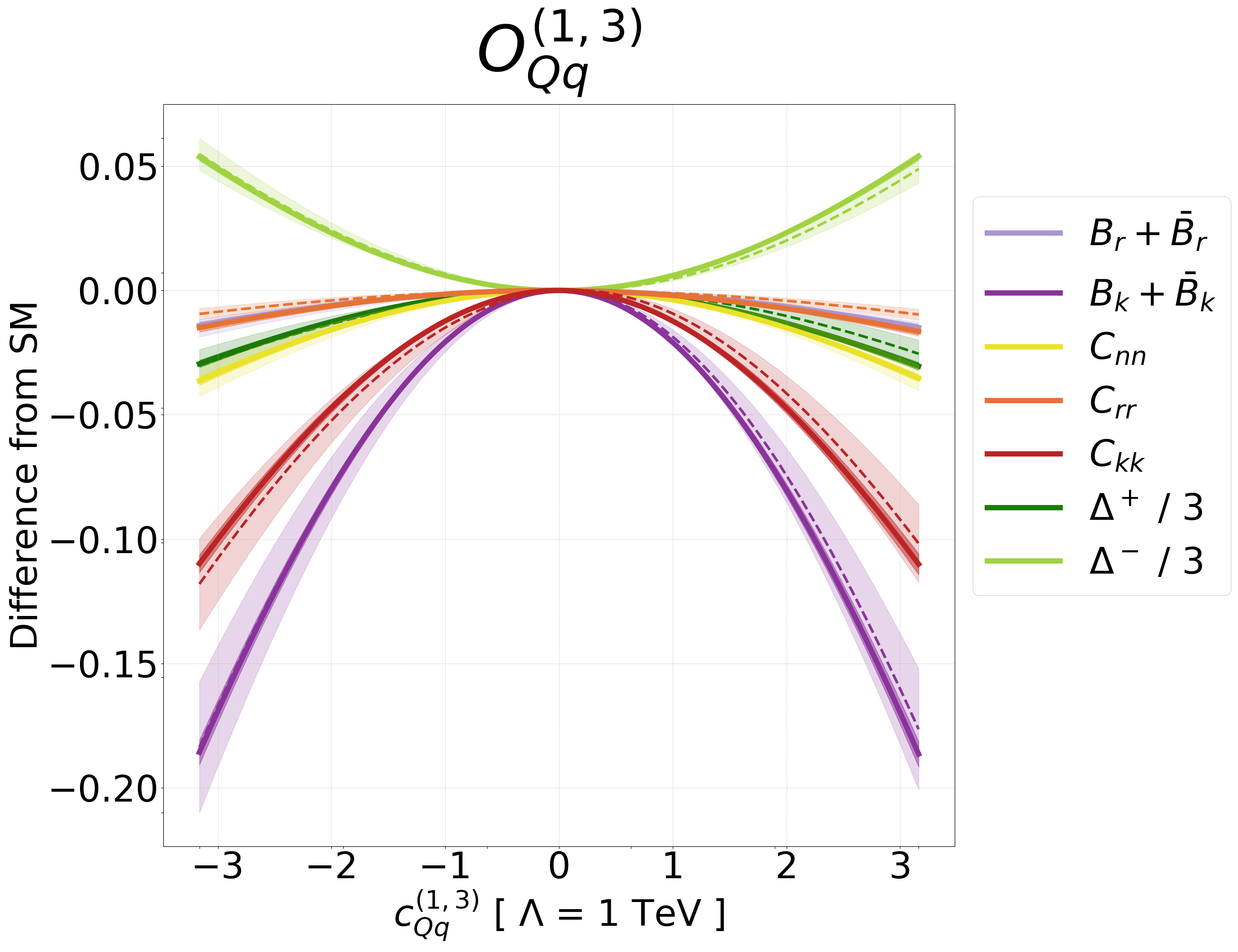
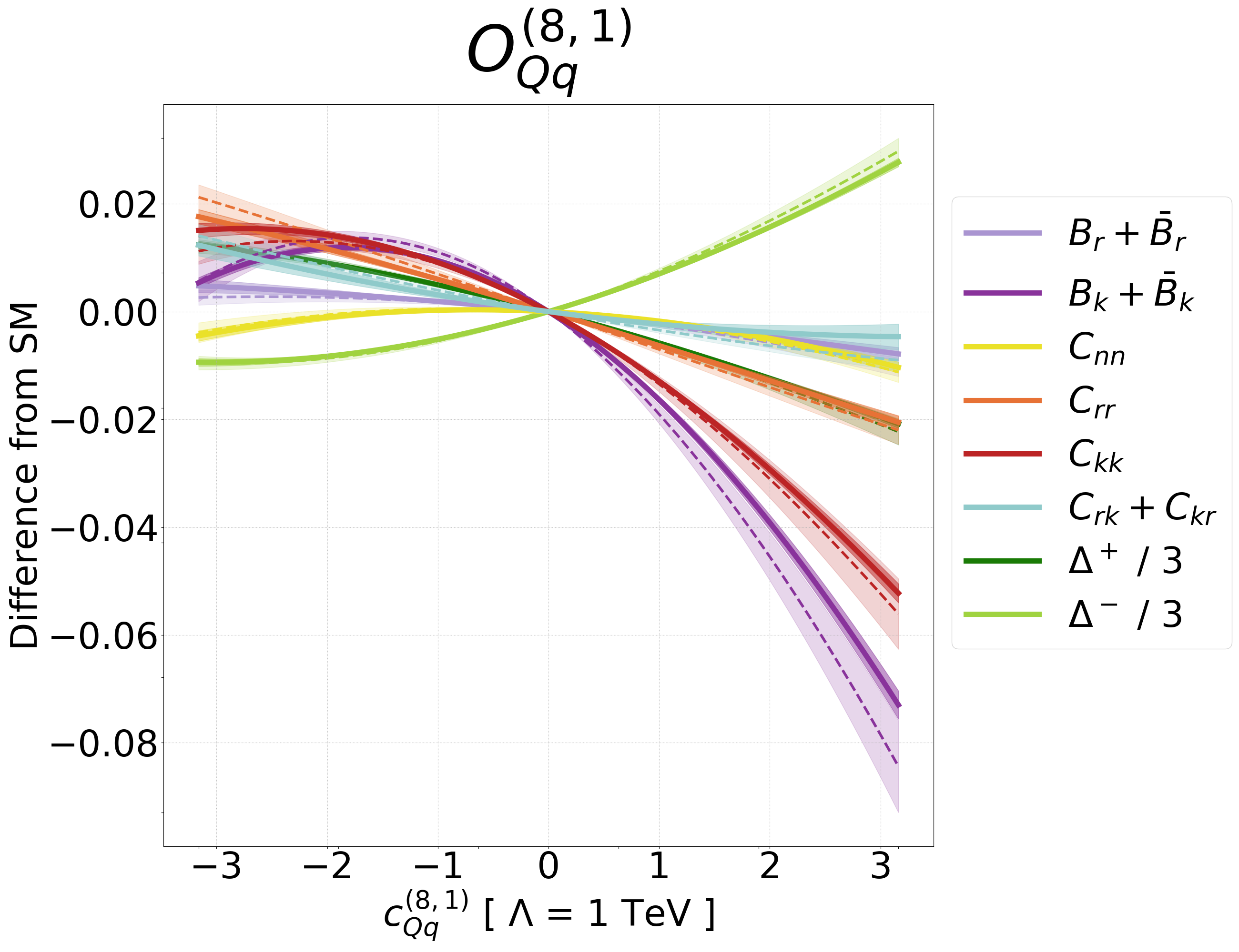
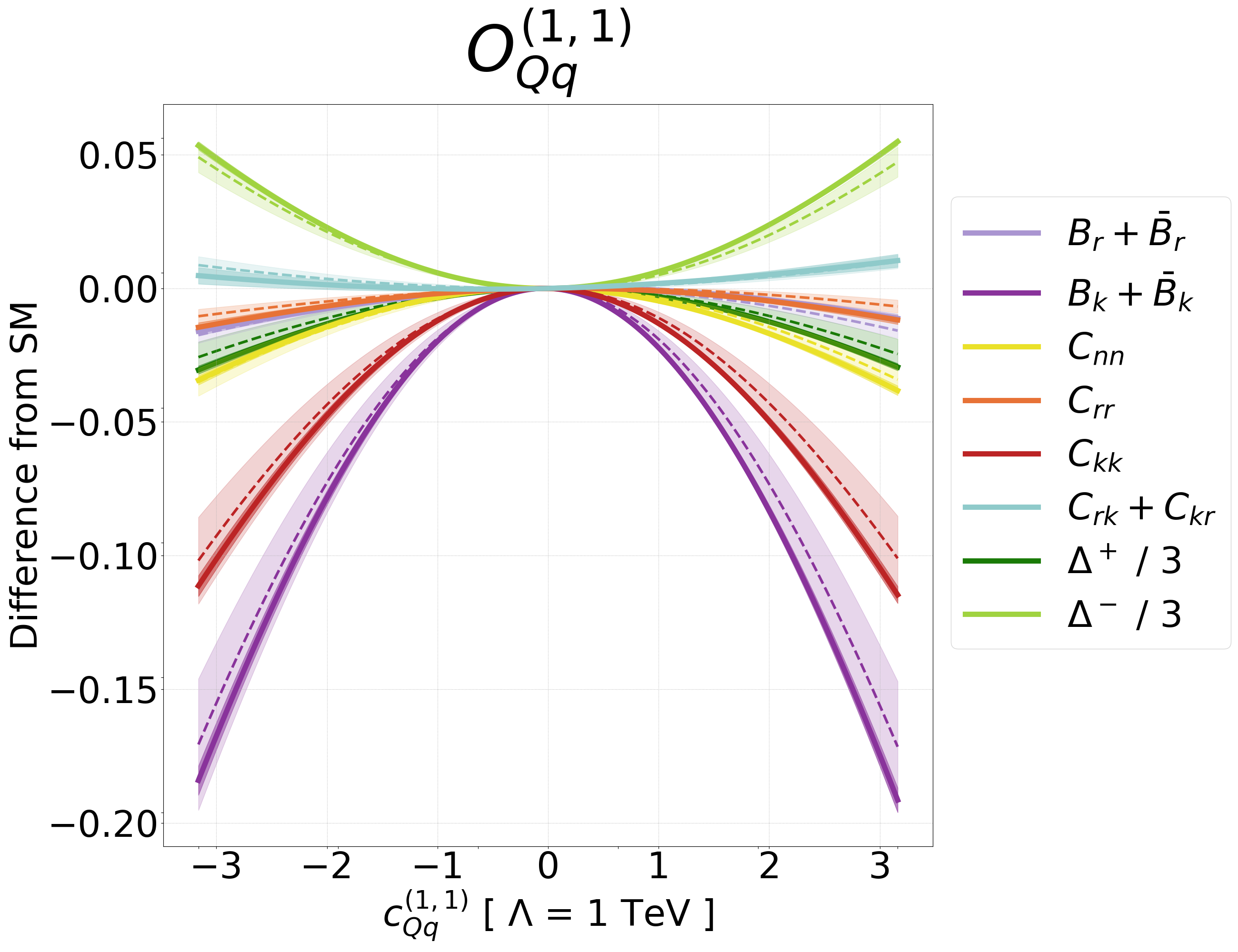
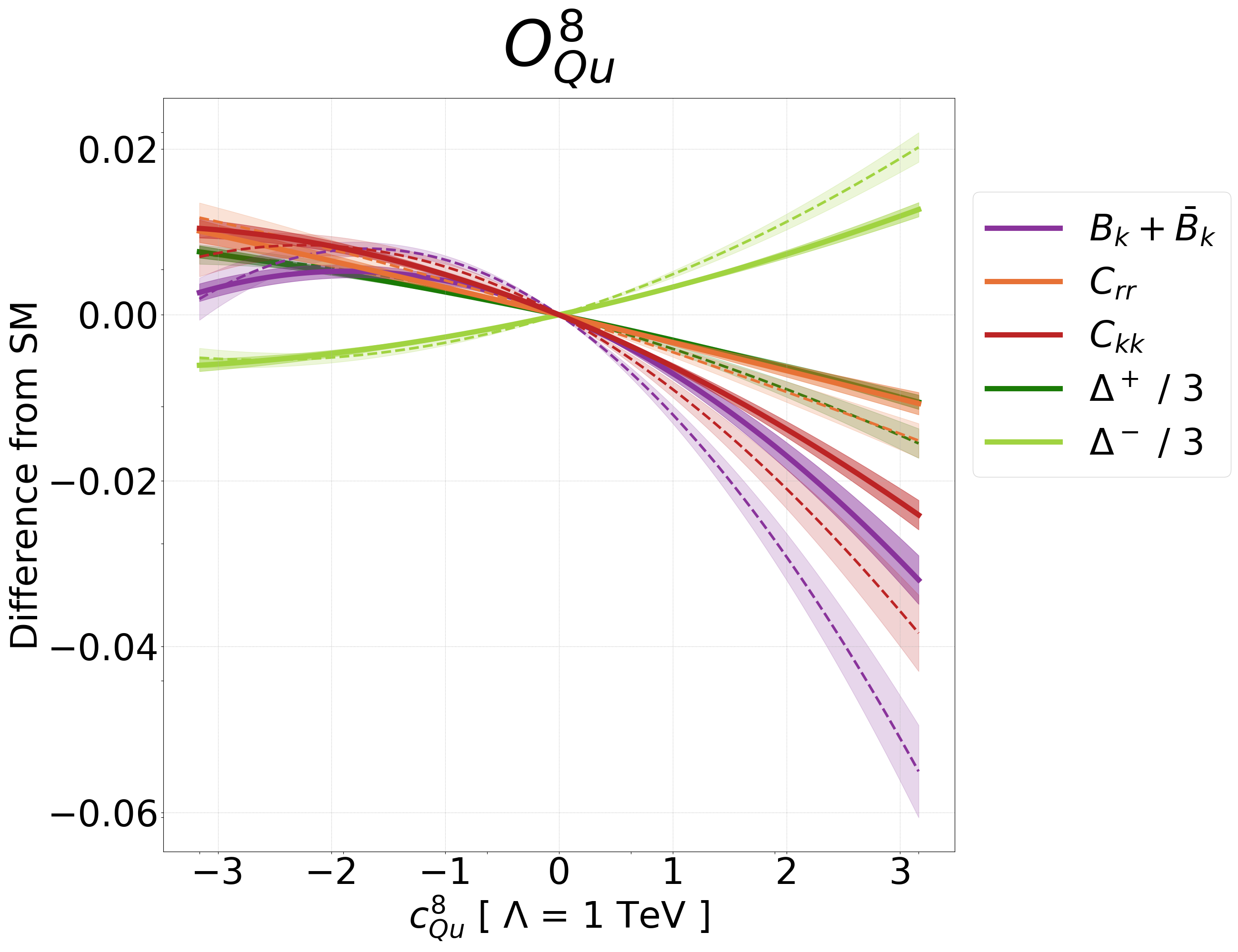
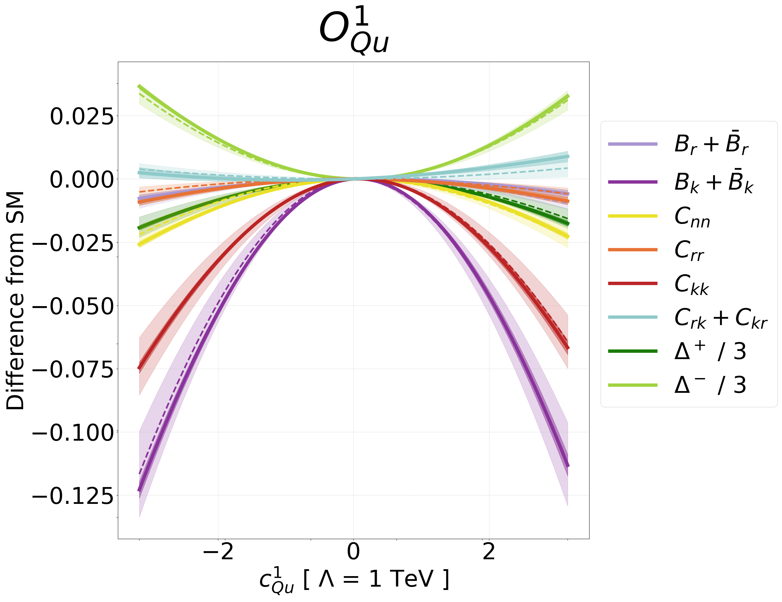
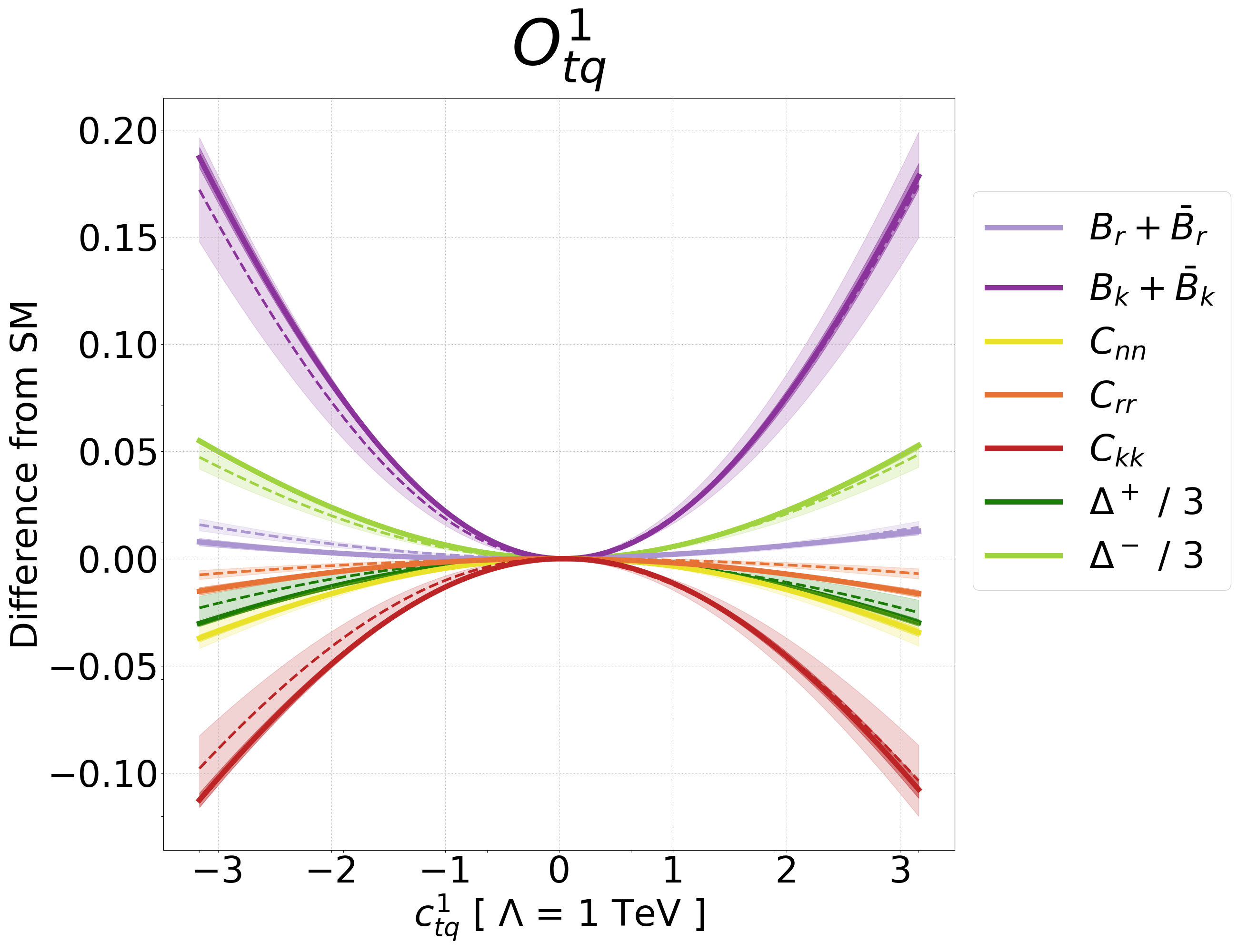
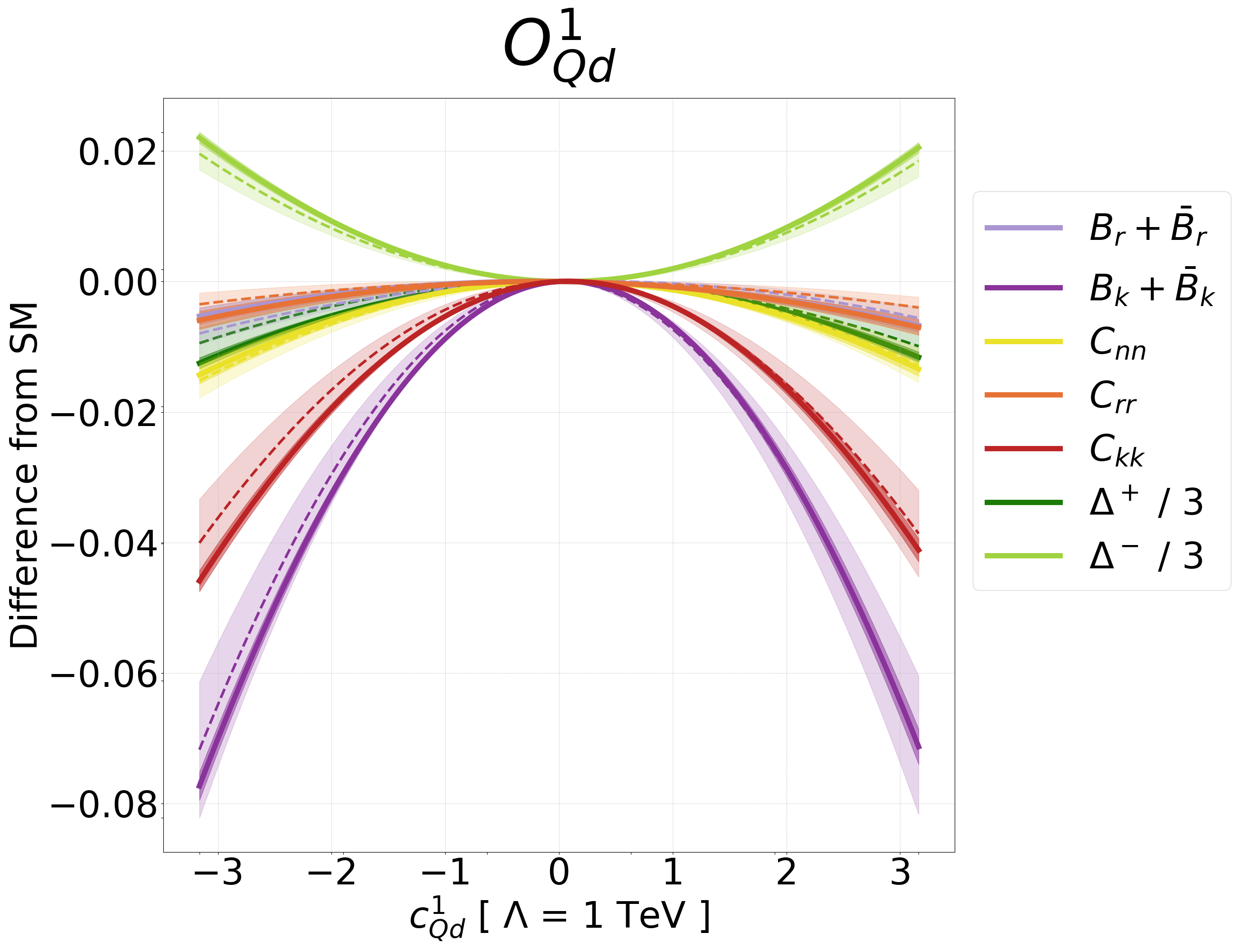
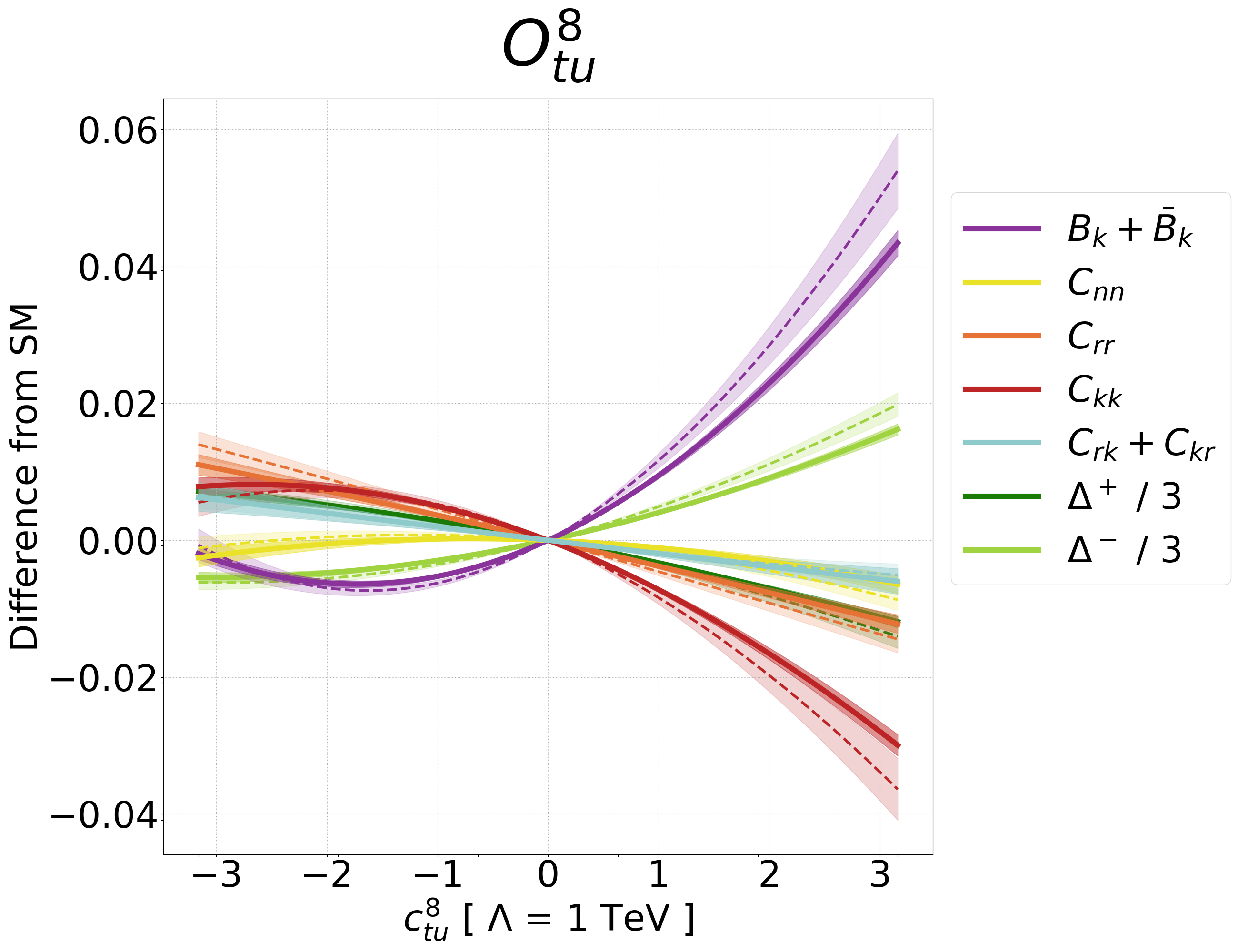
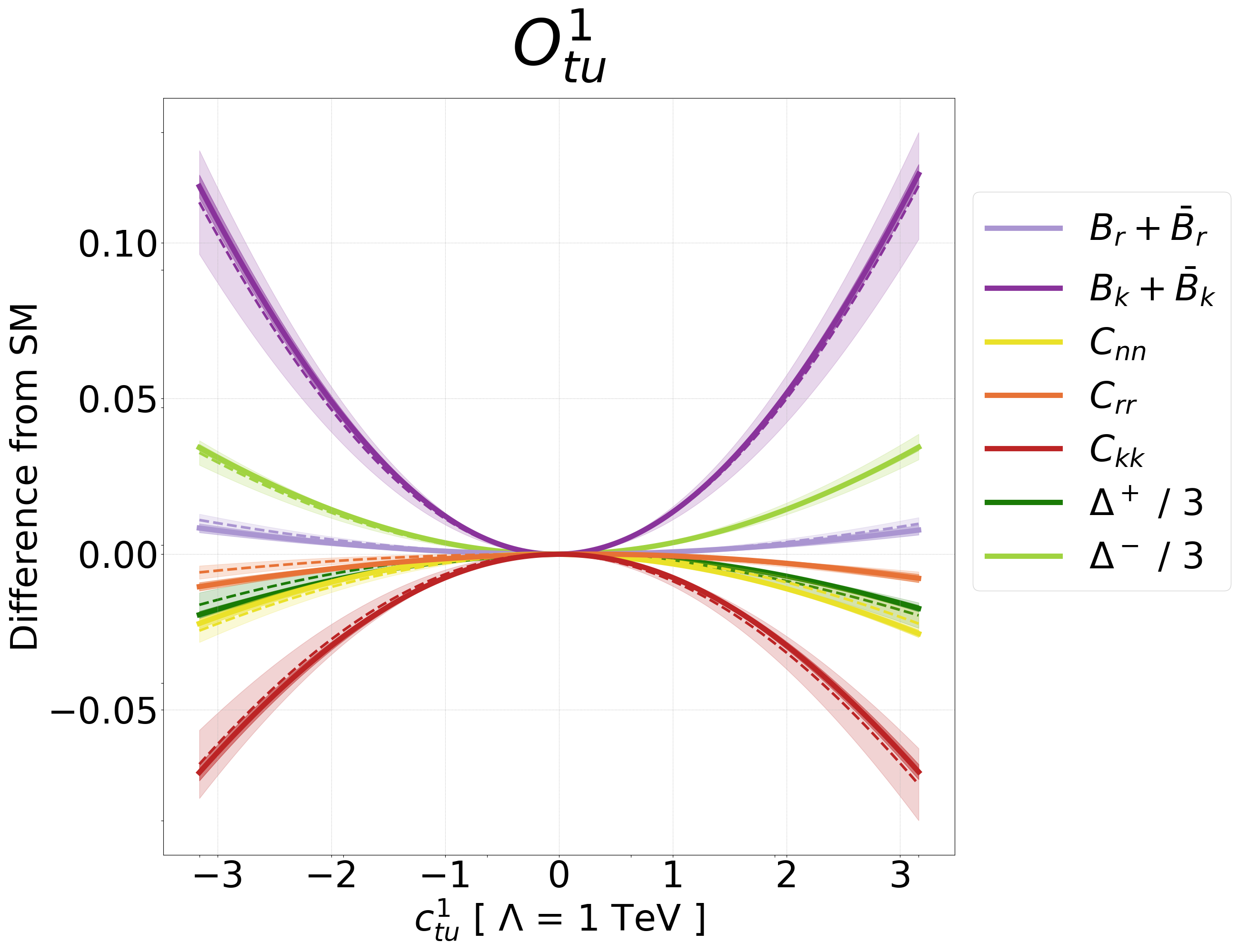
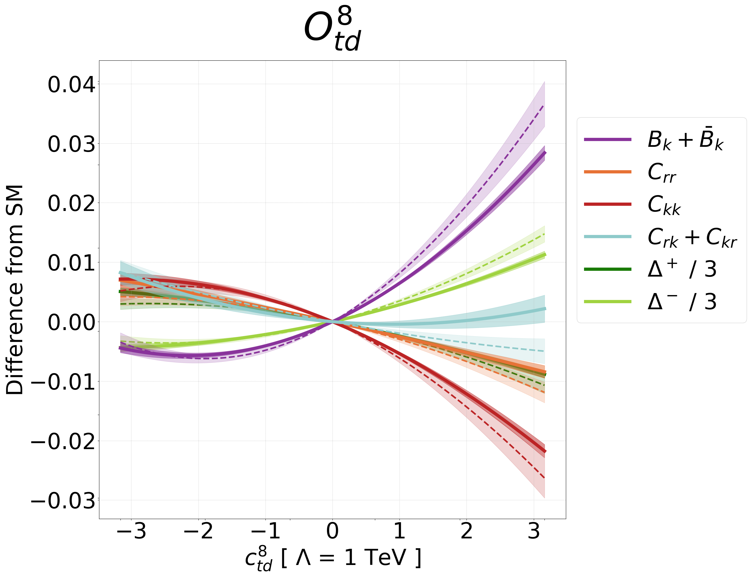
We begin by noting that quadratic terms 𝒪(c2/Λ4)𝒪superscript𝑐2superscriptΛ4\mathcal{O}(c^{2}/\Lambda^{4}), that induce a non-linear behaviour of spin observables, are almost always important, and often leading with respect to the SM-SMEFT interference 𝒪(c/Λ2)𝒪𝑐superscriptΛ2\mathcal{O}(c/\Lambda^{2}). This is particularly pronounced for the color-singlet operators for which the deviations from the SM are nearly identical for positive and negative values of the coefficients. This is expected as this class of operators only interferes with the SM at NLO in QCD. For the color-octet operators both linear and quadratic terms are important for the range of coefficients that we consider. We also notice that the effect of color-singlet operators is more prominent than the effect of color-octet operators, due to a relative color factor of 9/2929/2 entering the respective squared amplitudes.
Refer to caption
(a)
Refer to caption
(b)
Refer to caption
(c)
Refer to caption
(d)
Refer to caption
(e)
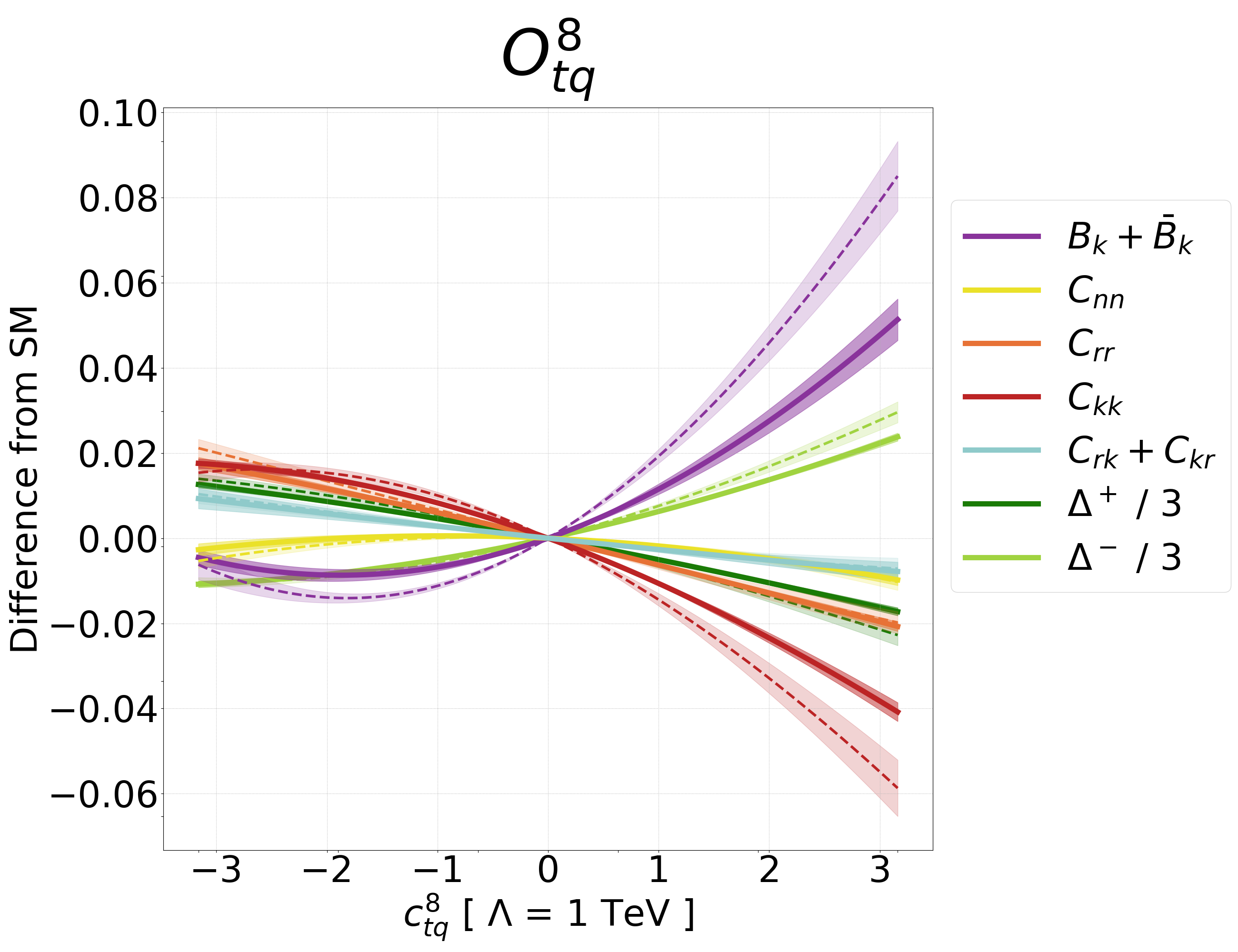
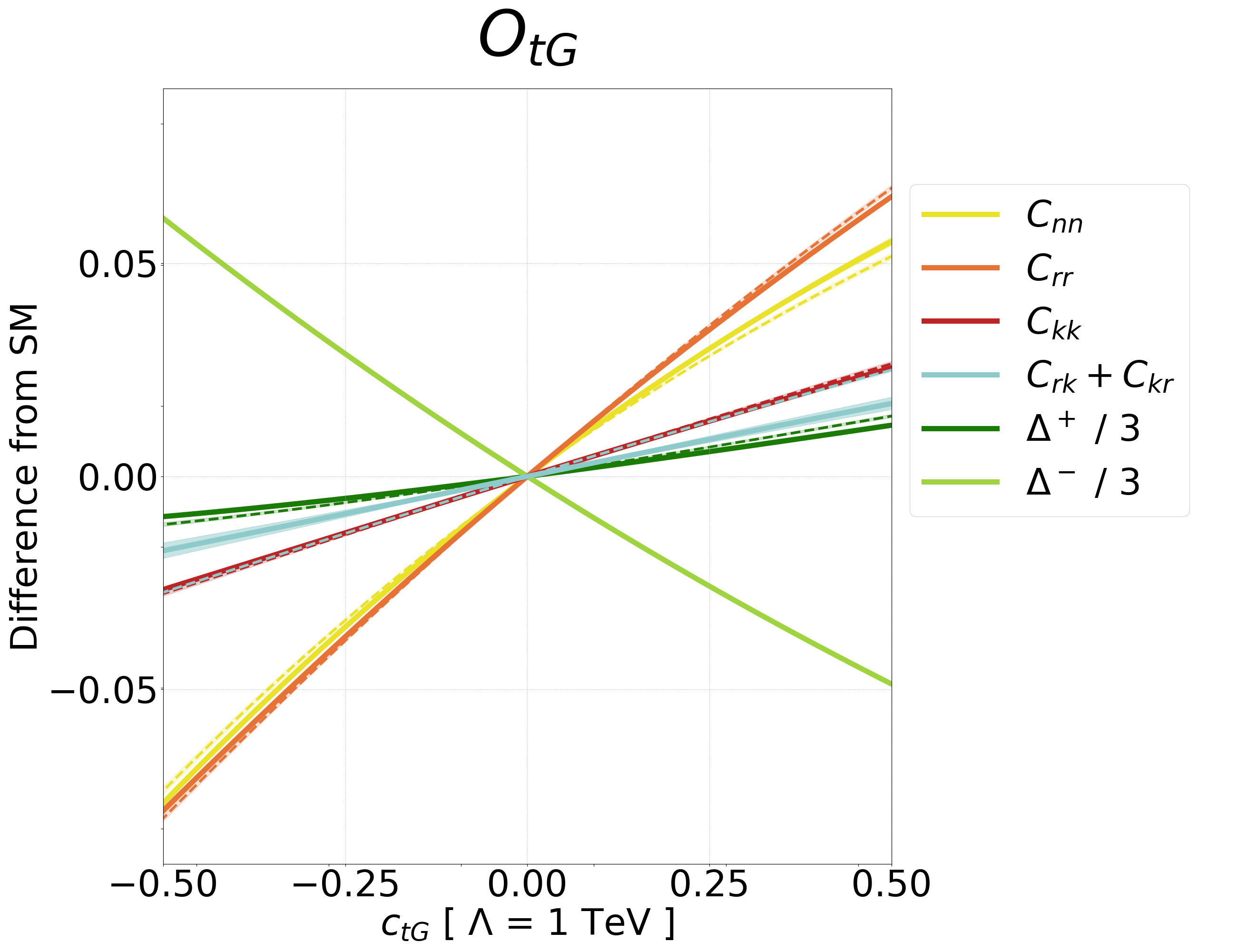
Figure 1: Change from the SM value for spin observables for the operators 𝒪tGsubscript𝒪𝑡𝐺\mathcal{O}_{tG} (1(a)), 𝒪Qq(8,3)superscriptsubscript𝒪𝑄𝑞83\mathcal{O}_{Qq}^{(8,3)} (1(b)), 𝒪Qq(1,3)superscriptsubscript𝒪𝑄𝑞13\mathcal{O}_{Qq}^{(1,3)} (1(c)), 𝒪Qq(8,1)superscriptsubscript𝒪𝑄𝑞81\mathcal{O}_{Qq}^{(8,1)} (1(d)), 𝒪Qq(1,1)superscriptsubscript𝒪𝑄𝑞11\mathcal{O}_{Qq}^{(1,1)} (1(e)), inclusive in tt¯𝑡¯𝑡t\bar{t} phase space. Dashed lines indicate results at LO, continuous lines indicate NLO. The shaded region around each curve represents the combination of scale and MC uncertainty. The MC uncertainty is always sub-leading compared to scale variation. Only curves that deviate appreciably from zero are shown.
Refer to caption
(a)
Refer to caption
(b)
Refer to caption
(c)
Refer to caption
(d)
Refer to caption
(e)
Refer to caption
(f)
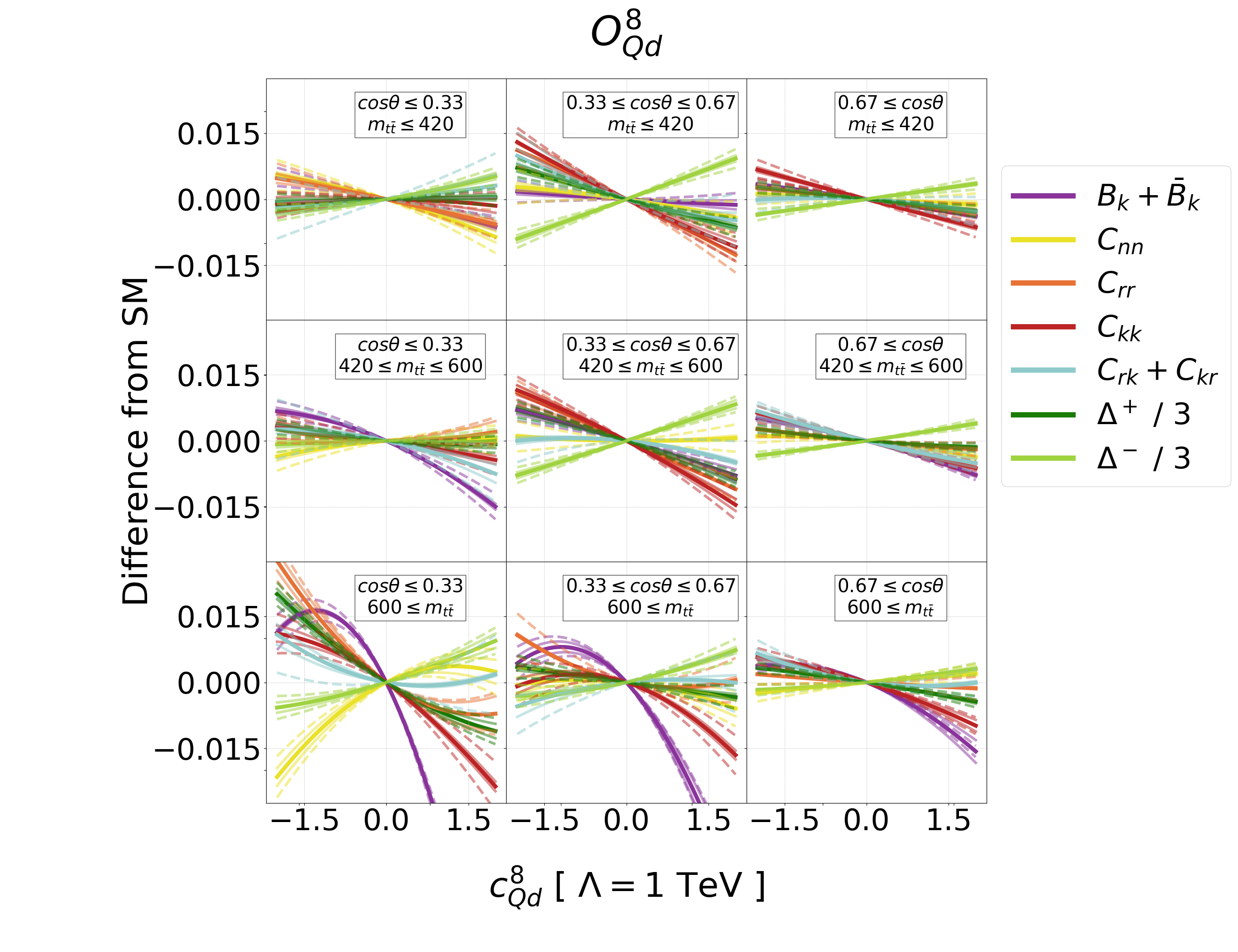
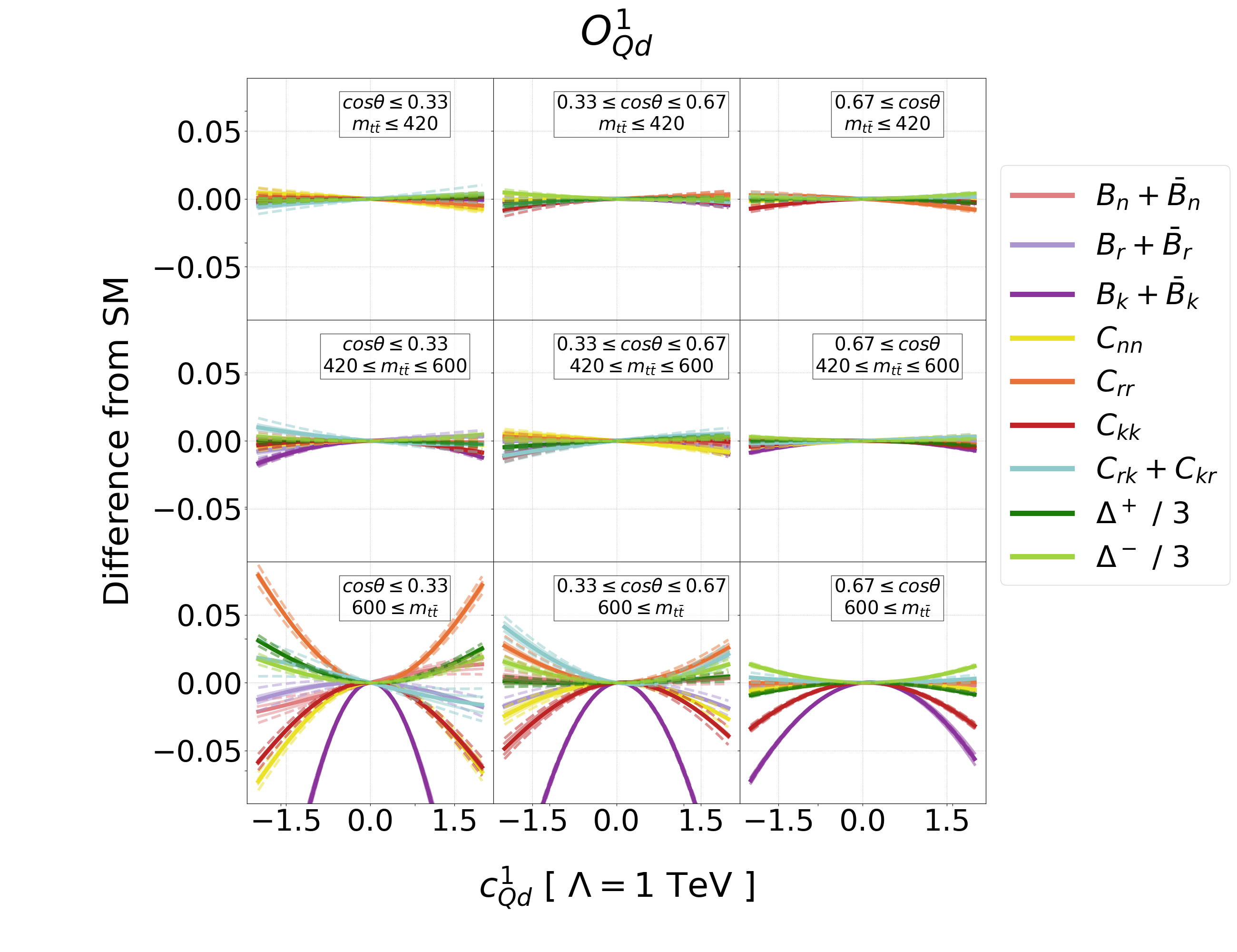
Figure 2: Results for the operators 𝒪Qu8superscriptsubscript𝒪𝑄𝑢8\mathcal{O}_{Qu}^{8} (2(a)), 𝒪Qu1superscriptsubscript𝒪𝑄𝑢1\mathcal{O}_{Qu}^{1} (2(b)), 𝒪tq8superscriptsubscript𝒪𝑡𝑞8\mathcal{O}_{tq}^{8} (2(c)), 𝒪tq1superscriptsubscript𝒪𝑡𝑞1\mathcal{O}_{tq}^{1} (2(d)), 𝒪Qd8superscriptsubscript𝒪𝑄𝑑8\mathcal{O}_{Qd}^{8} (2(e)) and 𝒪Qd1superscriptsubscript𝒪𝑄𝑑1\mathcal{O}_{Qd}^{1} (2(f)), similar to Figure 1.
Refer to caption
(a)
Refer to caption
(b)
Refer to caption
(c)
Refer to caption
(d)
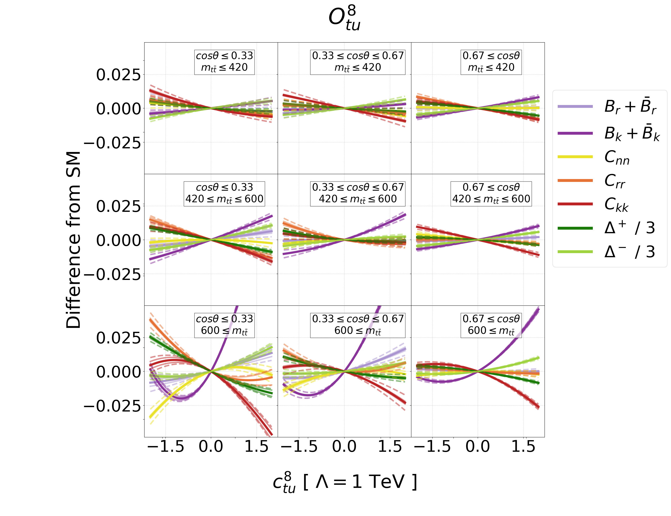
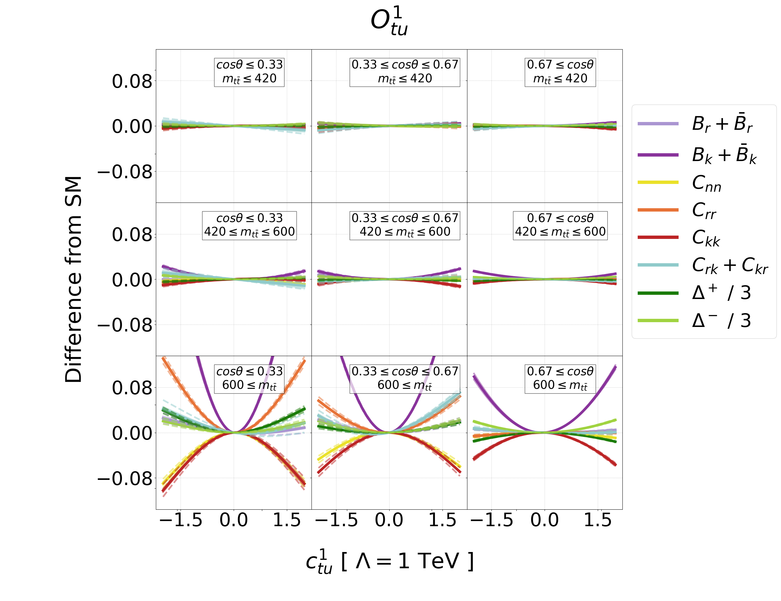
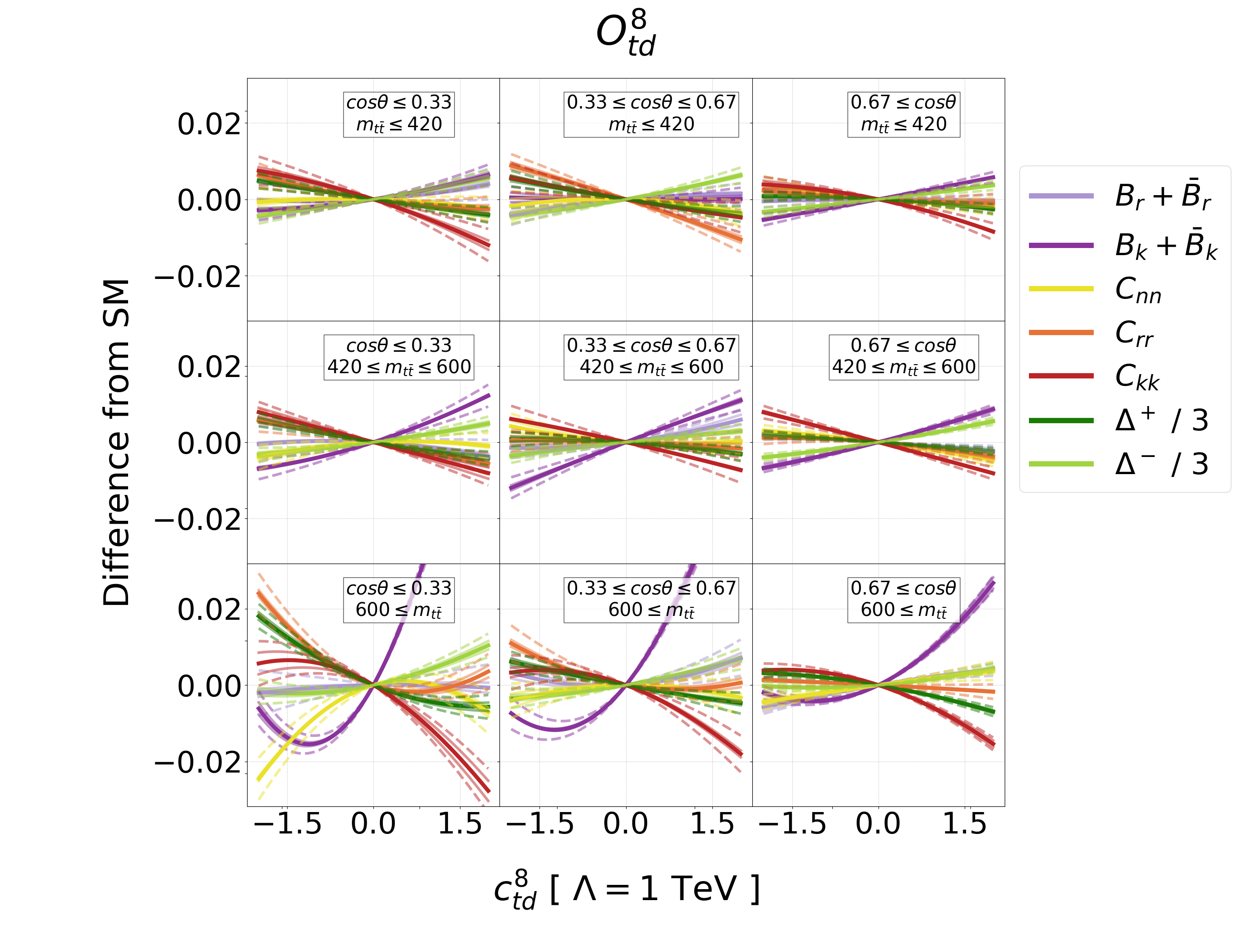
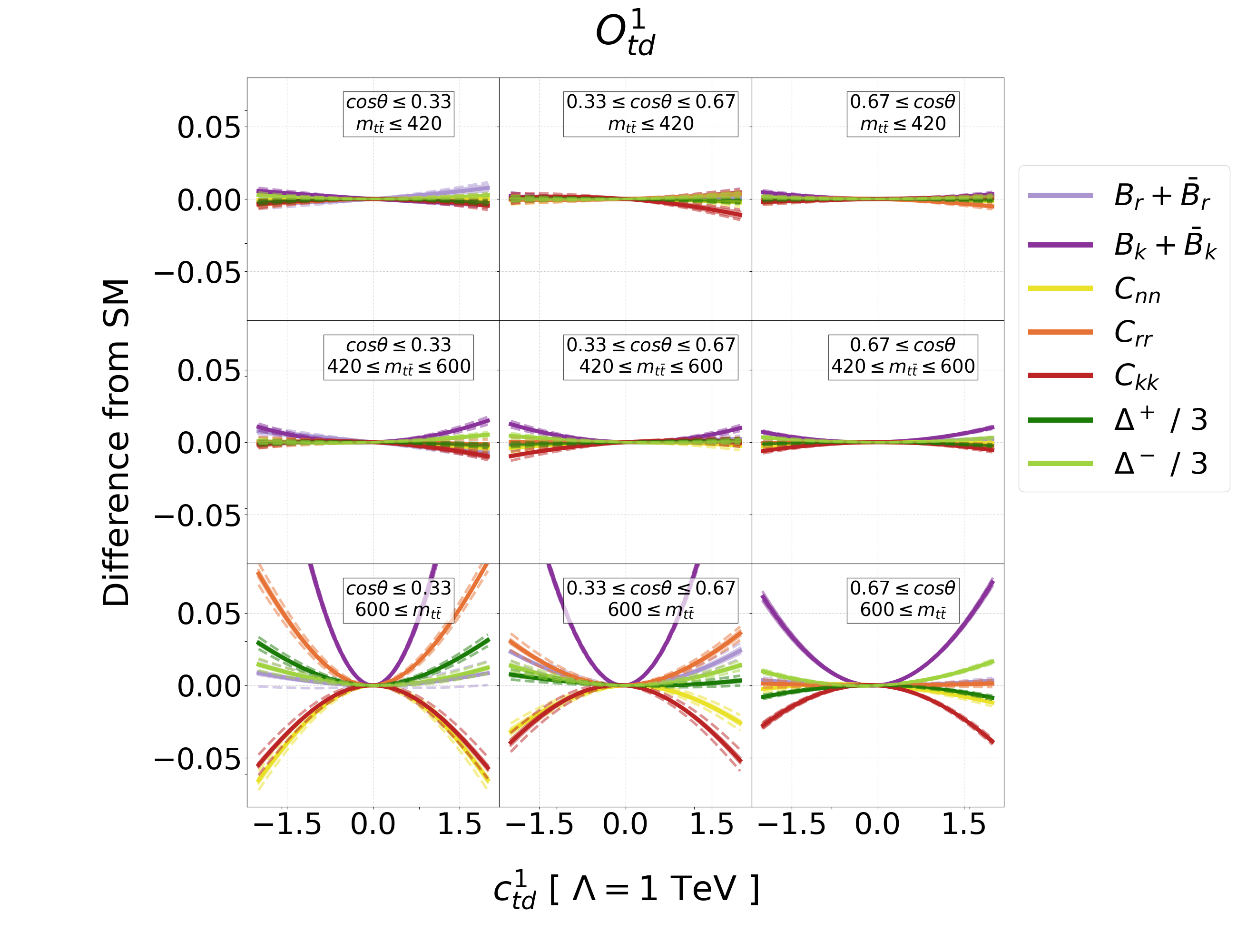
Figure 3: Results for the operators 𝒪tu8superscriptsubscript𝒪𝑡𝑢8\mathcal{O}_{tu}^{8} (3(a)), 𝒪tu1superscriptsubscript𝒪𝑡𝑢1\mathcal{O}_{tu}^{1} (3(b)), 𝒪td8superscriptsubscript𝒪𝑡𝑑8\mathcal{O}_{td}^{8} (3(c)), 𝒪td1superscriptsubscript𝒪𝑡𝑑1\mathcal{O}_{td}^{1} (3(d)), similar to Figure 1.

Our results are in qualitative agreement with the findings at LO QCD of Bernreuther:2015yna ; Aoude:2022imd , signaling that NLO QCD contributions are under control, and our curves appear stable under the inclusion of the NLO with 𝒪(10%)𝒪(αs)similar-to𝒪percent10𝒪subscript𝛼𝑠\mathcal{O}(10\%)\sim\mathcal{O}(\alpha_{s}) deviations. This is particularly true for spin correlation observables, as they arise from ratios of (weighted) cross-sections. It is frequently the case, however, that LO scale variation is not a good estimate for missing higher orders. This is especially true for color-octet operators, where the shift between LO QCD and NLO QCD often exceeds 3×3\times the LO scale variation. This is despite the fact that our scale variation is conservative, as it includes all nine points obtained from the 1/2,1,212121/2,1,2 rescaling of μRsubscript𝜇𝑅\mu_{R} and μfsubscript𝜇f\mu_{\text{f}}, and not the often used seven.

Looking at individual spin observables, we note that several are not affected by dimension-6 operators, even in the regime where the NP-squared terms are dominant. The n^^𝑛\hat{n} polarization Bn+B¯nsubscript𝐵𝑛subscript¯𝐵𝑛B_{n}+\overline{B}_{n} never deviates appreciably from its SM value for any of the operators we considered. This is because, as already noted in Aoude:2022imd , the only contributions to Bn+B¯nsubscript𝐵𝑛subscript¯𝐵𝑛B_{n}+\overline{B}_{n} come from the absorptive parts of one-loop amplitudes, and are thus heavily suppressed. Amongst those in Table 1, Bn+B¯nsubscript𝐵𝑛subscript¯𝐵𝑛B_{n}+\overline{B}_{n} is the only spin observable for which this happens.

The quantum entanglement markers Δ±superscriptΔplus-or-minus\Delta^{\pm} exhibit a similar pattern of deviations from the SM to the other spin observables. However, they are not included in this work for pure academic interest: their experimental measurement may be significantly simpler than the one of other observables. The enhanced precision is due to the fact that ΔsuperscriptΔ\Delta^{-} is accessible directly from the opening angle between the leptons, with no need for (3.11). The CMS Collaboration recently published a projection for top spin correlation measurements at the HL-LHC CMS:2022cqm , where it is argued that ΔsuperscriptΔ\Delta^{-} will be the spin observable more easily accessible, with a projected relative accuracy at the end of HL-LHC of 3%percent33\% 222The notation used in CMS:2022cqm and in other papers from experimental collaborations is D(Δ+1)/3𝐷superscriptΔ13D\equiv(\Delta^{-}+1)/3.. Given the prospects of precise measurements, the entanglement markers are expected to provide good sensitivity to the dimension-6 coefficients.

The top chromomagnetic moment operator 𝒪tGsubscript𝒪𝑡𝐺\mathcal{O}_{tG}.


Proceeding operator by operator, 𝒪tGsubscript𝒪𝑡𝐺\mathcal{O}_{tG} stands out as exhibiting a special behaviour. We immediately note that the effect of ctGsubscript𝑐𝑡𝐺c_{tG} is approximately ten times larger than the effect of all other four-fermion Wilson coefficients. Note the x𝑥x-axis scale of Fig. 1(a) is different from the one in all other plots. In fact, as noted below, top spin correlation measurements yield a remarkable sensitivity in constraining the value of ctGsubscript𝑐𝑡𝐺c_{tG}.

The large contribution of ctGsubscript𝑐𝑡𝐺c_{tG} to the spin observables we consider is a consequence of two factors. First, 𝒪tGsubscript𝒪𝑡𝐺\mathcal{O}_{tG} is the only SMEFT operator at dimension 6 that enters gluon-fusion top production ggtt¯𝑔𝑔𝑡¯𝑡g\,g\to t\,\bar{t}, and since σ(ggtt¯)/σ(qq¯tt¯)10similar-to𝜎𝑔𝑔𝑡¯𝑡𝜎𝑞¯𝑞𝑡¯𝑡10\sigma(g\,g\to t\,\bar{t})/\sigma(q\,\bar{q}\to t\,\bar{t})\sim 10 at the LHC, any BSM effect capable of entering gluon-fusion is heuristically expected to lead over those only appearing in qq¯𝑞¯𝑞q\bar{q} annihilation by a similar factor. Second, due to the nature of 𝒪tGsubscript𝒪𝑡𝐺\mathcal{O}_{tG}, the contributions proportional to ctGsubscript𝑐𝑡𝐺c_{tG} exhibit a structure that closely resembles the SM. In fact, the SM–𝒪tGsubscript𝒪𝑡𝐺\mathcal{O}_{tG} interference amplitude is numerically substantial, and addionally, as it can be seen from Table 5, the scale variation of ctGsubscript𝑐𝑡𝐺c_{tG} and SM cross-sections are highly correlated, and in fact cancel in the ratio when computing spin observables.

We also note that 𝒪tGsubscript𝒪𝑡𝐺\mathcal{O}_{tG} is affecting tt¯𝑡¯𝑡t\bar{t} spin correlations, that is entries of the Cijsubscript𝐶𝑖𝑗C_{ij} matrix, without modifying the SM values of each top’s polarization, Bisubscript𝐵𝑖B_{i} and B¯jsubscript¯𝐵𝑗\bar{B}_{j}. This is understood analytically, as both the linear and squared contribution of ctGsubscript𝑐𝑡𝐺c_{tG} to all polarization observables vanish at LO QCD.

A case study: Bk+B¯ksubscript𝐵𝑘subscript¯𝐵𝑘B_{k}+\overline{B}_{k}.


In the case of four-fermion operators, Bk+B¯ksubscript𝐵𝑘subscript¯𝐵𝑘B_{k}+\overline{B}_{k} is the spin observable that consistently deviates the most from its SM value. We therefore take it as a case study, and analyse its properties in detail. While an NLO-accurate analytical calculation of the SMEFT shifts of Bk+B¯ksubscript𝐵𝑘subscript¯𝐵𝑘B_{k}+\overline{B}_{k} is laborious, and beyond the scope of this work, interesting patterns emerge from our numerical results, shown in App. A for all observables, and reported in Table 3 for the reader’s convenience.

As noted above, 𝒪tGsubscript𝒪𝑡𝐺\mathcal{O}_{tG} does not contribute significantly to Bk+B¯ksubscript𝐵𝑘subscript¯𝐵𝑘B_{k}+\bar{B}_{k}. The four-fermion operators, that all contribute, can be grouped in two classes, 𝒪Qq(8,3),𝒪Qq(8,1),𝒪Qu8,𝒪Qd8superscriptsubscript𝒪𝑄𝑞83superscriptsubscript𝒪𝑄𝑞81superscriptsubscript𝒪𝑄𝑢8superscriptsubscript𝒪𝑄𝑑8\mathcal{O}_{Qq}^{(8,3)},\mathcal{O}_{Qq}^{(8,1)},\mathcal{O}_{Qu}^{8},\mathcal{O}_{Qd}^{8}, for which the SM shift is negative, and 𝒪tq8,𝒪tu8,𝒪td8superscriptsubscript𝒪𝑡𝑞8superscriptsubscript𝒪𝑡𝑢8superscriptsubscript𝒪𝑡𝑑8\mathcal{O}_{tq}^{8},\mathcal{O}_{tu}^{8},\mathcal{O}_{td}^{8}, for which the shift is positive. In the following we will focus on color-octet operators, but our exact arguments apply to color-singlet operators.

At order c/Λ2𝑐superscriptΛ2c/\Lambda^{2}, the trend of positive/negative shifts with respect to the SM is consistent with the phase space integration of the results presented in Aoude:2022imd , where it is noted that at LO QCD the coupling of new physics to Bk+B¯ksubscript𝐵𝑘subscript¯𝐵𝑘B_{k}+\overline{B}_{k}, at linear order, is only through the Axial-Vector (AV) combinations:

cQq(8,3)cQq(8,1)cQu8+ctq8+ctu8,subscriptsuperscript𝑐83𝑄𝑞superscriptsubscript𝑐𝑄𝑞81superscriptsubscript𝑐𝑄𝑢8superscriptsubscript𝑐𝑡𝑞8superscriptsubscript𝑐𝑡𝑢8\displaystyle-c^{(8,3)}_{Qq}-c_{Qq}^{(8,1)}-c_{Qu}^{8}+c_{tq}^{8}+c_{tu}^{8},\quad for uu¯tt¯for 𝑢¯𝑢𝑡¯𝑡\displaystyle\text{for }u\bar{u}\to t\bar{t} (5.2)
cQq(8,3)cQq(8,1)cQd8+ctq8+ctd8,subscriptsuperscript𝑐83𝑄𝑞superscriptsubscript𝑐𝑄𝑞81superscriptsubscript𝑐𝑄𝑑8superscriptsubscript𝑐𝑡𝑞8superscriptsubscript𝑐𝑡𝑑8\displaystyle c^{(8,3)}_{Qq}-c_{Qq}^{(8,1)}-c_{Qd}^{8}+c_{tq}^{8}+c_{td}^{8},\quad for dd¯tt¯.for 𝑑¯𝑑𝑡¯𝑡\displaystyle\text{for }d\bar{d}\to t\bar{t}. (5.3)

The coefficient cQq(8,3)subscriptsuperscript𝑐83𝑄𝑞c^{(8,3)}_{Qq} enters with opposite signs the uu¯𝑢¯𝑢u\bar{u} and dd¯𝑑¯𝑑d\bar{d} processes; the fact that the uu¯𝑢¯𝑢u\bar{u} contribution is observed to dominate in our numerical calculation, as shown in Figure 1(b), is of course understood in terms of PDF luminosity in pp𝑝𝑝p\,p collisions.

Color-octet Color-singlet
Operators Order σ(1)superscript𝜎1\sigma^{(1)} [pb] σ(2)superscript𝜎2\sigma^{(2)} [pb] σ(1)superscript𝜎1\sigma^{(1)} [pb] σ(2)superscript𝜎2\sigma^{(2)} [pb]
𝒪Qq(8,3)superscriptsubscript𝒪𝑄𝑞83\mathcal{O}_{Qq}^{(8,3)} and 𝒪Qq(1,3)superscriptsubscript𝒪𝑄𝑞13\mathcal{O}_{Qq}^{(1,3)} LO 0.079(10)0.011+0.008-0.079\scriptstyle{(10)}\,\displaystyle{{}^{+0.008}_{-0.011}} 0.133(3)0.013+0.011-0.133\scriptstyle{(3)}\,\displaystyle{{}^{+0.011}_{-0.013}} 0.036(23)0.008+0.0070.036\scriptstyle{(23)}\,\displaystyle{{}^{+0.007}_{-0.008}} 0.584(5)0.043+0.038-0.584\scriptstyle{(5)}\,\displaystyle{{}^{+0.038}_{-0.043}}
NLO 0.083(7)0.001+0.004-0.083\scriptstyle{(7)}\,\displaystyle{{}^{+0.004}_{-0.001}} 0.118(2)0.001+0.002-0.118\scriptstyle{(2)}\,\displaystyle{{}^{+0.002}_{-0.001}} 0.004(16)0.004+0.007-0.004\scriptstyle{(16)}\,\displaystyle{{}^{+0.007}_{-0.004}} 0.761(4)0.034+0.031-0.761\scriptstyle{(4)}\,\displaystyle{{}^{+0.031}_{-0.034}}
𝒪Qq(8,1)superscriptsubscript𝒪𝑄𝑞81\mathcal{O}_{Qq}^{(8,1)} and 𝒪Qq(1,1)superscriptsubscript𝒪𝑄𝑞11\mathcal{O}_{Qq}^{(1,1)} LO 0.441(10)0.068+0.054-0.441\scriptstyle{(10)}\,\displaystyle{{}^{+0.054}_{-0.068}} 0.123(3)0.011+0.009-0.123\scriptstyle{(3)}\,\displaystyle{{}^{+0.009}_{-0.011}} 0.004(28)0.001+0.000-0.004\scriptstyle{(28)}\,\displaystyle{{}^{+0.000}_{-0.001}} 0.557(7)0.040+0.035-0.557\scriptstyle{(7)}\,\displaystyle{{}^{+0.035}_{-0.040}}
NLO 0.469(7)0.003+0.014-0.469\scriptstyle{(7)}\,\displaystyle{{}^{+0.014}_{-0.003}} 0.129(2)0.003+0.003-0.129\scriptstyle{(2)}\,\displaystyle{{}^{+0.003}_{-0.003}} 0.044(14)0.015+0.011-0.044\scriptstyle{(14)}\,\displaystyle{{}^{+0.011}_{-0.015}} 0.767(4)0.035+0.032-0.767\scriptstyle{(4)}\,\displaystyle{{}^{+0.032}_{-0.035}}
𝒪Qu8superscriptsubscript𝒪𝑄𝑢8\mathcal{O}_{Qu}^{8} and 𝒪Qu1superscriptsubscript𝒪𝑄𝑢1\mathcal{O}_{Qu}^{1} LO 0.272(8)0.043+0.034-0.272\scriptstyle{(8)}\,\displaystyle{{}^{+0.034}_{-0.043}} 0.080(2)0.008+0.006-0.080\scriptstyle{(2)}\,\displaystyle{{}^{+0.006}_{-0.008}} 0.019(16)0.002+0.0020.019\scriptstyle{(16)}\,\displaystyle{{}^{+0.002}_{-0.002}} 0.357(4)0.026+0.023-0.357\scriptstyle{(4)}\,\displaystyle{{}^{+0.023}_{-0.026}}
NLO 0.203(7)0.009+0.021-0.203\scriptstyle{(7)}\,\displaystyle{{}^{+0.021}_{-0.009}} 0.055(2)0.003+0.004-0.055\scriptstyle{(2)}\,\displaystyle{{}^{+0.004}_{-0.003}} 0.062(10)0.012+0.0170.062\scriptstyle{(10)}\,\displaystyle{{}^{+0.017}_{-0.012}} 0.462(2)0.020+0.018-0.462\scriptstyle{(2)}\,\displaystyle{{}^{+0.018}_{-0.020}}
𝒪tq8superscriptsubscript𝒪𝑡𝑞8\mathcal{O}_{tq}^{8} and 𝒪tq1superscriptsubscript𝒪𝑡𝑞1\mathcal{O}_{tq}^{1} LO 0.446(10)0.057+0.0730.446\scriptstyle{(10)}\,\displaystyle{{}^{+0.073}_{-0.057}} 0.123(2)0.010+0.0120.123\scriptstyle{(2)}\,\displaystyle{{}^{+0.012}_{-0.010}} 0.012(28)0.002+0.0020.012\scriptstyle{(28)}\,\displaystyle{{}^{+0.002}_{-0.002}} 0.562(6)0.036+0.0420.562\scriptstyle{(6)}\,\displaystyle{{}^{+0.042}_{-0.036}}
NLO 0.332(7)0.043+0.0160.332\scriptstyle{(7)}\,\displaystyle{{}^{+0.016}_{-0.043}} 0.089(2)0.006+0.0040.089\scriptstyle{(2)}\,\displaystyle{{}^{+0.004}_{-0.006}} 0.062(15)0.019+0.014-0.062\scriptstyle{(15)}\,\displaystyle{{}^{+0.014}_{-0.019}} 0.747(3)0.029+0.0310.747\scriptstyle{(3)}\,\displaystyle{{}^{+0.031}_{-0.029}}
𝒪Qd8superscriptsubscript𝒪𝑄𝑑8\mathcal{O}_{Qd}^{8} and 𝒪Qd1superscriptsubscript𝒪𝑄𝑑1\mathcal{O}_{Qd}^{1} LO 0.195(6)0.034+0.026-0.195\scriptstyle{(6)}\,\displaystyle{{}^{+0.026}_{-0.034}} 0.049(2)0.005+0.004-0.049\scriptstyle{(2)}\,\displaystyle{{}^{+0.004}_{-0.005}} 0.003(11)0.002+0.0020.003\scriptstyle{(11)}\,\displaystyle{{}^{+0.002}_{-0.002}} 0.217(3)0.017+0.015-0.217\scriptstyle{(3)}\,\displaystyle{{}^{+0.015}_{-0.017}}
NLO 0.150(7)0.008+0.017-0.150\scriptstyle{(7)}\,\displaystyle{{}^{+0.017}_{-0.008}} 0.033(2)0.002+0.003-0.033\scriptstyle{(2)}\,\displaystyle{{}^{+0.003}_{-0.002}} 0.036(8)0.007+0.0080.036\scriptstyle{(8)}\,\displaystyle{{}^{+0.008}_{-0.007}} 0.282(2)0.012+0.011-0.282\scriptstyle{(2)}\,\displaystyle{{}^{+0.011}_{-0.012}}
𝒪tu8superscriptsubscript𝒪𝑡𝑢8\mathcal{O}_{tu}^{8} and 𝒪tu1superscriptsubscript𝒪𝑡𝑢1\mathcal{O}_{tu}^{1} LO 0.262(9)0.032+0.0400.262\scriptstyle{(9)}\,\displaystyle{{}^{+0.040}_{-0.032}} 0.081(2)0.007+0.0080.081\scriptstyle{(2)}\,\displaystyle{{}^{+0.008}_{-0.007}} 0.026(17)0.003+0.0040.026\scriptstyle{(17)}\,\displaystyle{{}^{+0.004}_{-0.003}} 0.360(4)0.023+0.0260.360\scriptstyle{(4)}\,\displaystyle{{}^{+0.026}_{-0.023}}
NLO 0.268(7)0.008+0.0020.268\scriptstyle{(7)}\,\displaystyle{{}^{+0.002}_{-0.008}} 0.078(2)0.001+0.0020.078\scriptstyle{(2)}\,\displaystyle{{}^{+0.002}_{-0.001}} 0.024(11)0.007+0.0110.024\scriptstyle{(11)}\,\displaystyle{{}^{+0.011}_{-0.007}} 0.471(3)0.020+0.0230.471\scriptstyle{(3)}\,\displaystyle{{}^{+0.023}_{-0.020}}
𝒪td8superscriptsubscript𝒪𝑡𝑑8\mathcal{O}_{td}^{8} and 𝒪td1superscriptsubscript𝒪𝑡𝑑1\mathcal{O}_{td}^{1} LO 0.188(9)0.023+0.0290.188\scriptstyle{(9)}\,\displaystyle{{}^{+0.029}_{-0.023}} 0.050(2)0.004+0.0050.050\scriptstyle{(2)}\,\displaystyle{{}^{+0.005}_{-0.004}} 0.005(10)0.002+0.001-0.005\scriptstyle{(10)}\,\displaystyle{{}^{+0.001}_{-0.002}} 0.215(3)0.014+0.0160.215\scriptstyle{(3)}\,\displaystyle{{}^{+0.016}_{-0.014}}
NLO 0.191(7)0.007+0.0050.191\scriptstyle{(7)}\,\displaystyle{{}^{+0.005}_{-0.007}} 0.044(2)0.000+0.0010.044\scriptstyle{(2)}\,\displaystyle{{}^{+0.001}_{-0.000}} 0.020(9)0.004+0.0050.020\scriptstyle{(9)}\,\displaystyle{{}^{+0.005}_{-0.004}} 0.288(2)0.013+0.0150.288\scriptstyle{(2)}\,\displaystyle{{}^{+0.015}_{-0.013}}
Table 3: Cross sections appearing in the numerator of (3.13) for Bk+B¯ksubscript𝐵𝑘subscript¯𝐵𝑘B_{k}+\bar{B}_{k} for the four-fermion operators we consider in this work, extracted from Appendix A and with the same notation, central(stat)scale+scalesubscriptsuperscriptcentral(stat)scalescale\text{central(stat)}^{+\text{scale}}_{-\text{scale}}

At order 𝒪(c2/Λ4)𝒪superscript𝑐2superscriptΛ4\mathcal{O}(c^{2}/\Lambda^{4}) and LO QCD, a calculation based on FeynCalc Shtabovenko:2020gxv and the SMEFTatNLO model Degrande:2020evl shows that new physics enters in Bk+B¯ksubscript𝐵𝑘subscript¯𝐵𝑘B_{k}+\overline{B}_{k} through the combinations:

(cQq(8,3)+cQq(8,1))2(cQu8)2+(ctq8)2+(ctu8)2,superscriptsubscriptsuperscript𝑐83𝑄𝑞superscriptsubscript𝑐𝑄𝑞812superscriptsuperscriptsubscript𝑐𝑄𝑢82superscriptsuperscriptsubscript𝑐𝑡𝑞82superscriptsuperscriptsubscript𝑐𝑡𝑢82\displaystyle-(c^{(8,3)}_{Qq}+c_{Qq}^{(8,1)})^{2}-(c_{Qu}^{8})^{2}+(c_{tq}^{8})^{2}+(c_{tu}^{8})^{2},\quad for uu¯tt¯,for 𝑢¯𝑢𝑡¯𝑡\displaystyle\text{for }u\bar{u}\to t\bar{t}, (5.4)
(cQq(8,3)+cQq(8,1))2(cQd8)2+(ctq8)2+(ctd8)2,superscriptsubscriptsuperscript𝑐83𝑄𝑞superscriptsubscript𝑐𝑄𝑞812superscriptsuperscriptsubscript𝑐𝑄𝑑82superscriptsuperscriptsubscript𝑐𝑡𝑞82superscriptsuperscriptsubscript𝑐𝑡𝑑82\displaystyle-(-c^{(8,3)}_{Qq}+c_{Qq}^{(8,1)})^{2}-(c_{Qd}^{8})^{2}+(c_{tq}^{8})^{2}+(c_{td}^{8})^{2},\quad for dd¯tt¯,for 𝑑¯𝑑𝑡¯𝑡\displaystyle\text{for }d\bar{d}\to t\bar{t}, (5.5)

when no phase-space cuts are applied on the tt¯𝑡¯𝑡t\bar{t} pair. This is confirmed by our numerical results in Table 3. The relative signs between four-fermion operators that enter the contributions to Bk+B¯ksubscript𝐵𝑘subscript¯𝐵𝑘B_{k}+\overline{B}_{k} at linear and quadratic order in c/Λ2𝑐superscriptΛ2c/\Lambda^{2} are not the same as those that enter in the total tt¯𝑡¯𝑡t\bar{t} cross-section. For instance, at LO QCD and linearly in c/Λ2𝑐superscriptΛ2c/\Lambda^{2}, the inclusive cross section is only sensitive to the Vector-Vector (VV) combination Bernreuther:2015yna ; Aoude:2022imd :

cQq(8,3)+cQq(8,1)+cQu8+ctq8+ctu8.subscriptsuperscript𝑐83𝑄𝑞superscriptsubscript𝑐𝑄𝑞81superscriptsubscript𝑐𝑄𝑢8superscriptsubscript𝑐𝑡𝑞8superscriptsubscript𝑐𝑡𝑢8\displaystyle c^{(8,3)}_{Qq}+c_{Qq}^{(8,1)}+c_{Qu}^{8}+c_{tq}^{8}+c_{tu}^{8}. (5.6)

At quadratic SMEFT order 𝒪(c2/Λ4)𝒪superscript𝑐2superscriptΛ4\mathcal{O}(c^{2}/\Lambda^{4}) more combinations of Wilson coefficients enter the inclusive cross section, but, again, not the specific ones in (5.4) and (5.5). This simple observation already highlights the importance of spin observables in breaking flat directions otherwise present in the 4-fermion sector.

We also note that several operators exhibit a relatively large K𝐾K-factor between the LO and NLO. Most notably, 𝒪Qu8superscriptsubscript𝒪𝑄𝑢8\mathcal{O}_{Qu}^{8}, 𝒪tq8superscriptsubscript𝒪𝑡𝑞8\mathcal{O}_{tq}^{8}, and 𝒪Qd8superscriptsubscript𝒪𝑄𝑑8\mathcal{O}_{Qd}^{8}, show a 50%similar-toabsentpercent50\sim 50\% decrease in the σ(2)superscript𝜎2\sigma^{(2)} cross-section when going to NLO. This in turn translates to a significant mismatch between the LO and NLO curves in Figures 2(a), 2(c), and 2(e), that is not predicted by the LO scale variation.

We conclude this Section with a remark: the difference from the SM values for all spin observables we considered is of order 0.10.10.1 over the range of Wilson coefficients still allowed by the 2021 global fit Ethier:2021bye . The measurement of spin polarizations and spin correlations in a hadron collider is notoriously difficult, and a %percent\% level precision, needed to be competitive on the global fit, may be out of reach. However, as we shall see in the next section, the elaborate structure of spin observables in tt¯𝑡¯𝑡t\bar{t} phase space suggests a different route.

5.2 Results differential in tt¯𝑡¯𝑡t\bar{t} phase space

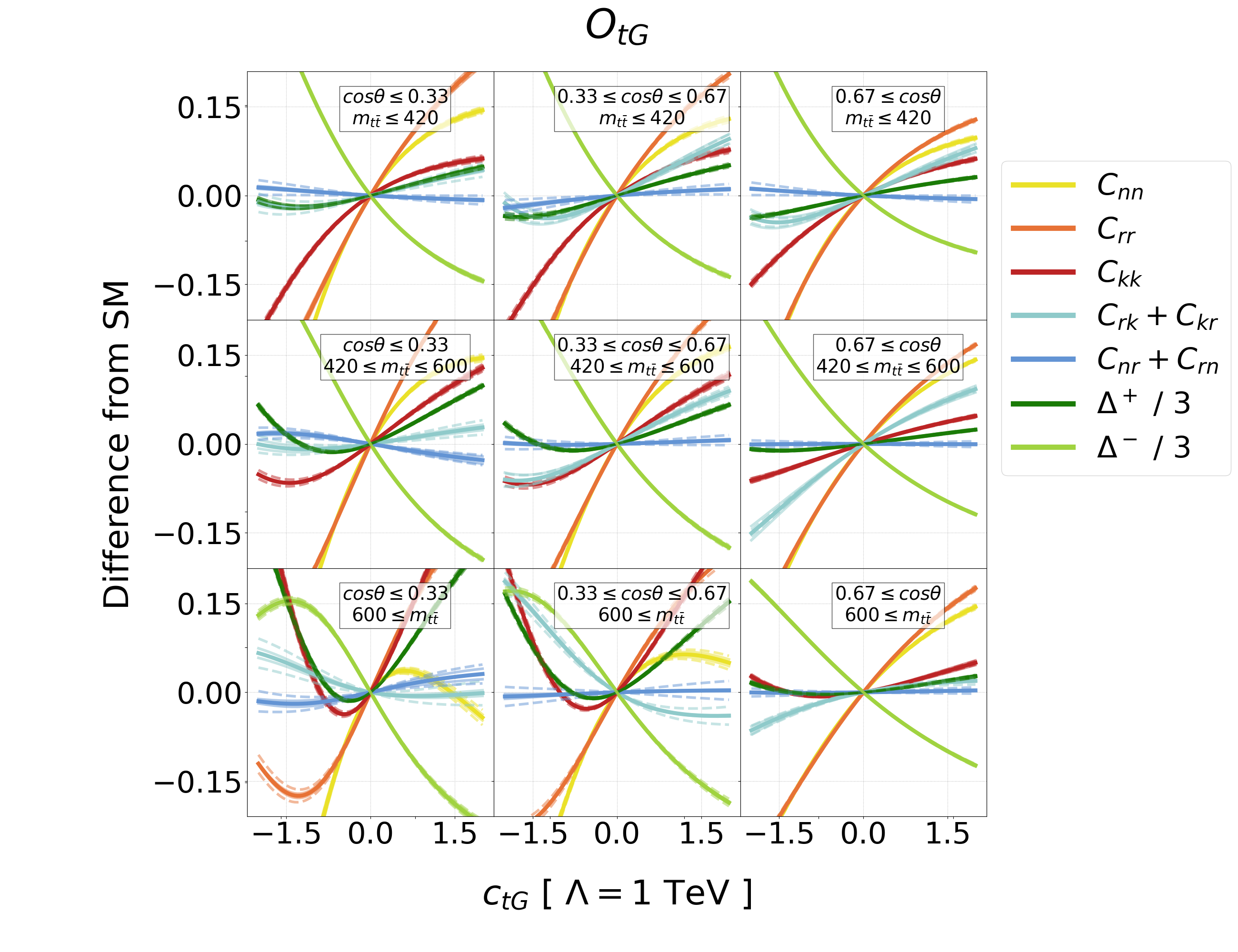
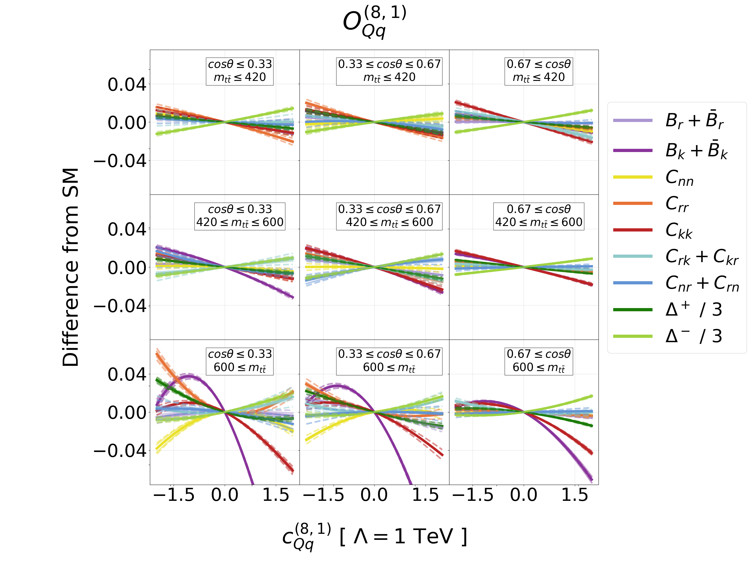
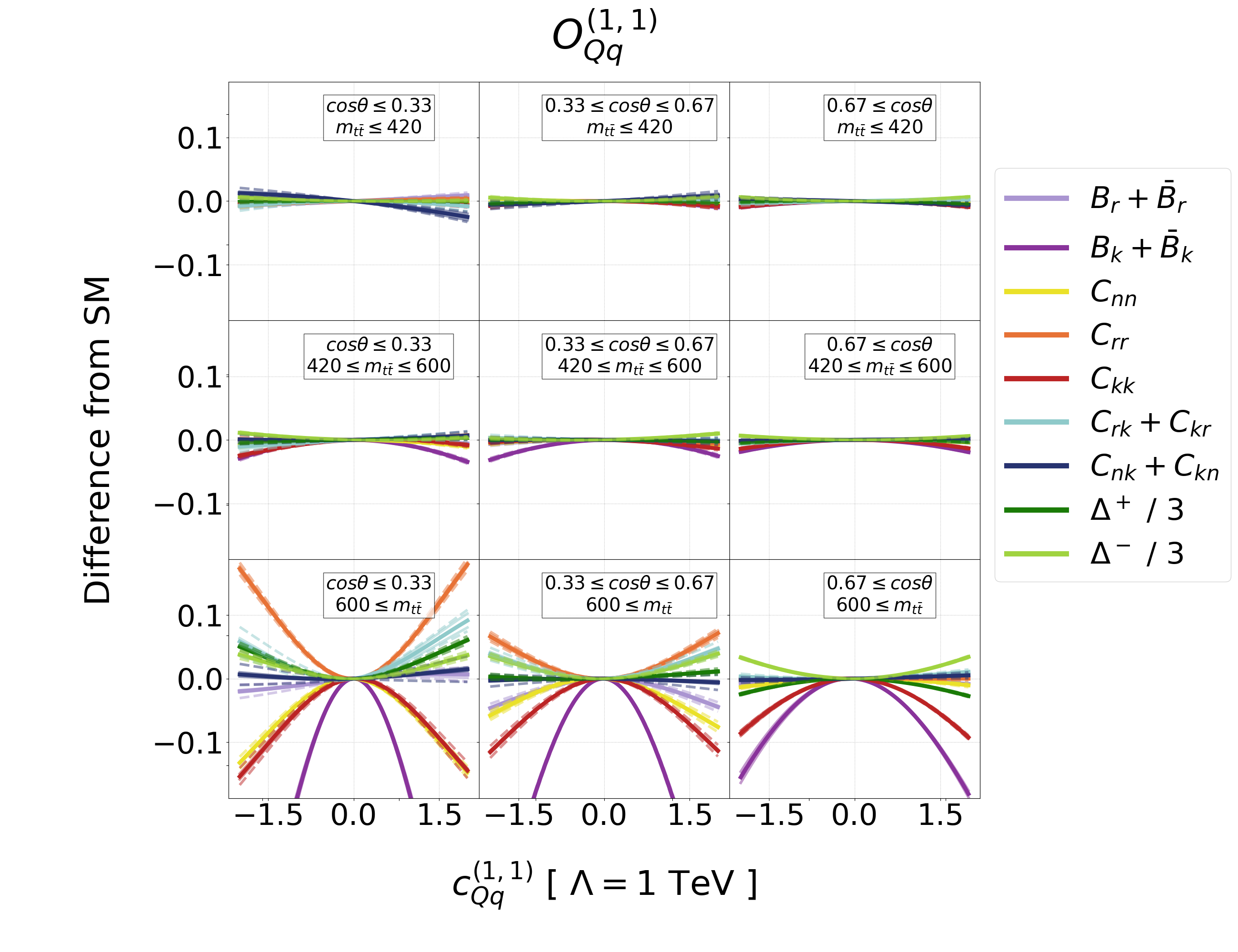
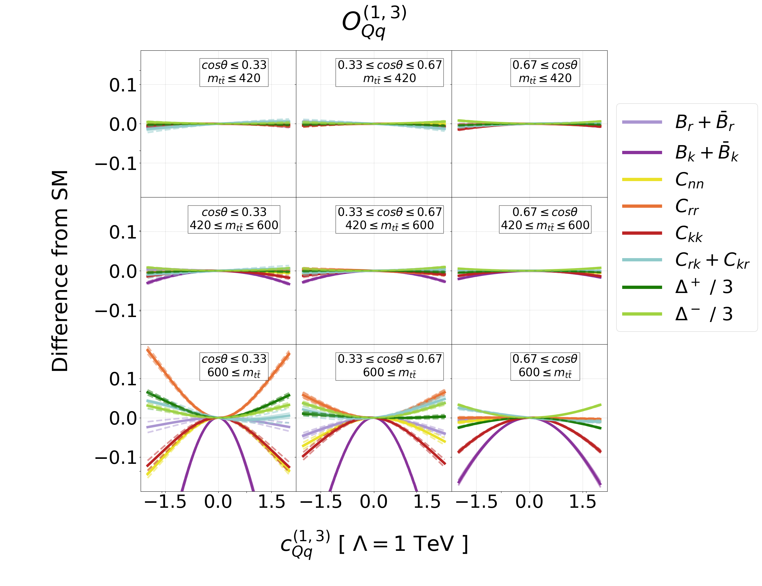
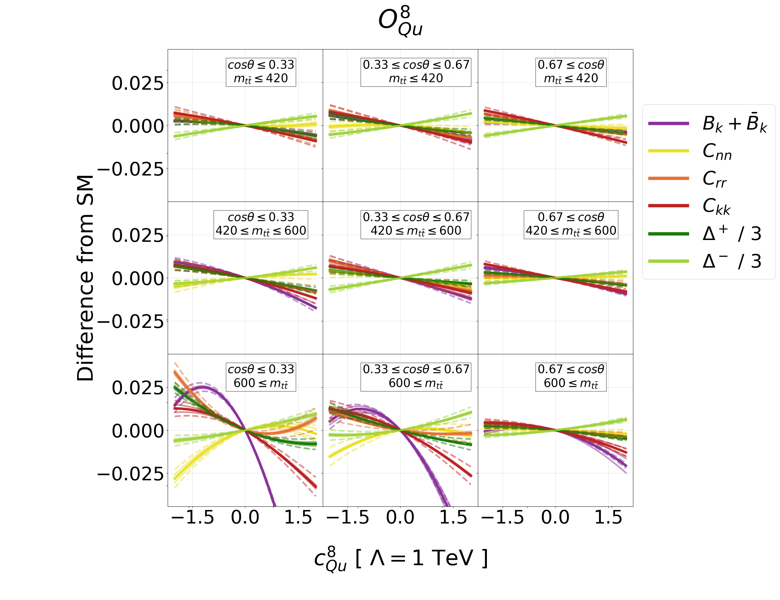
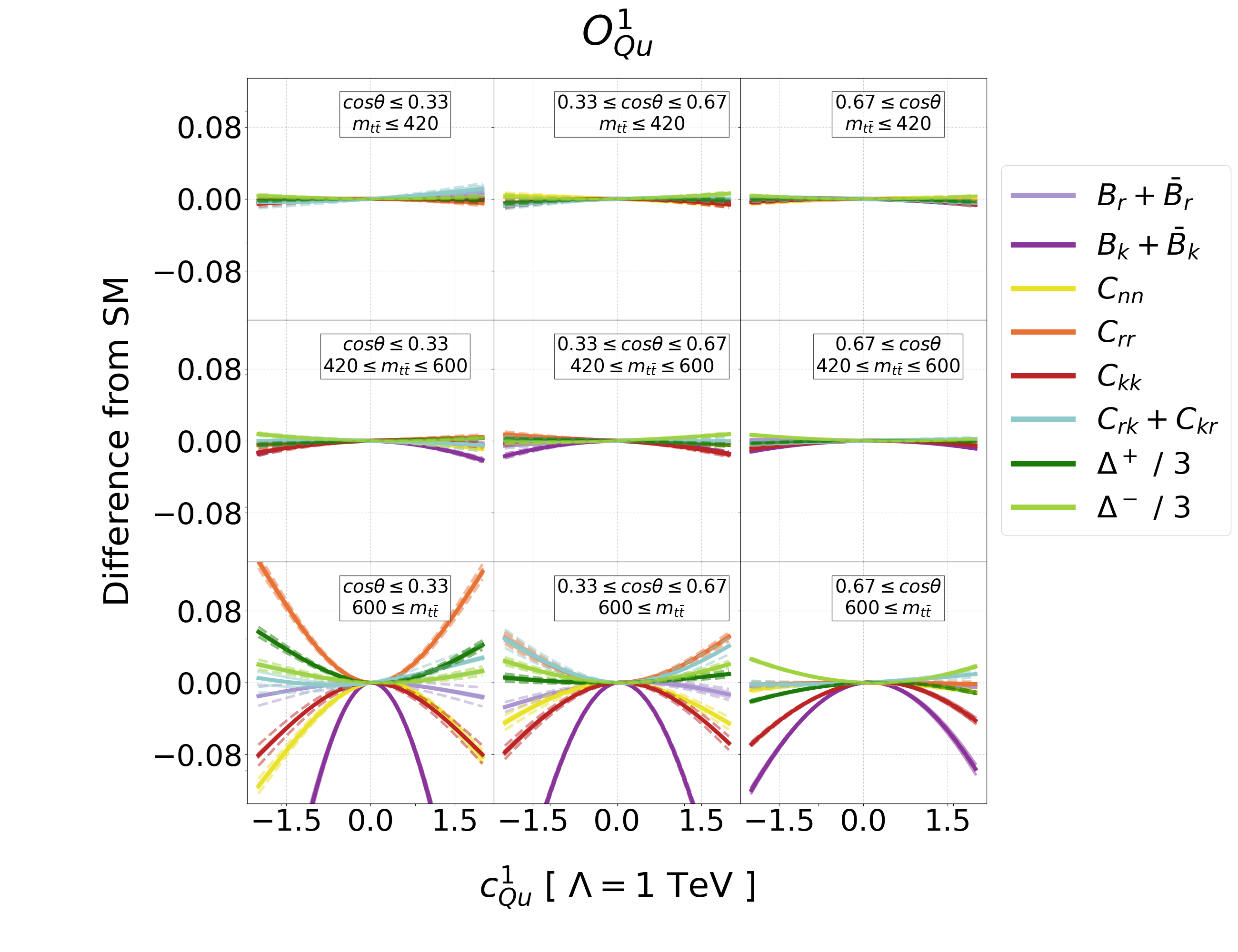
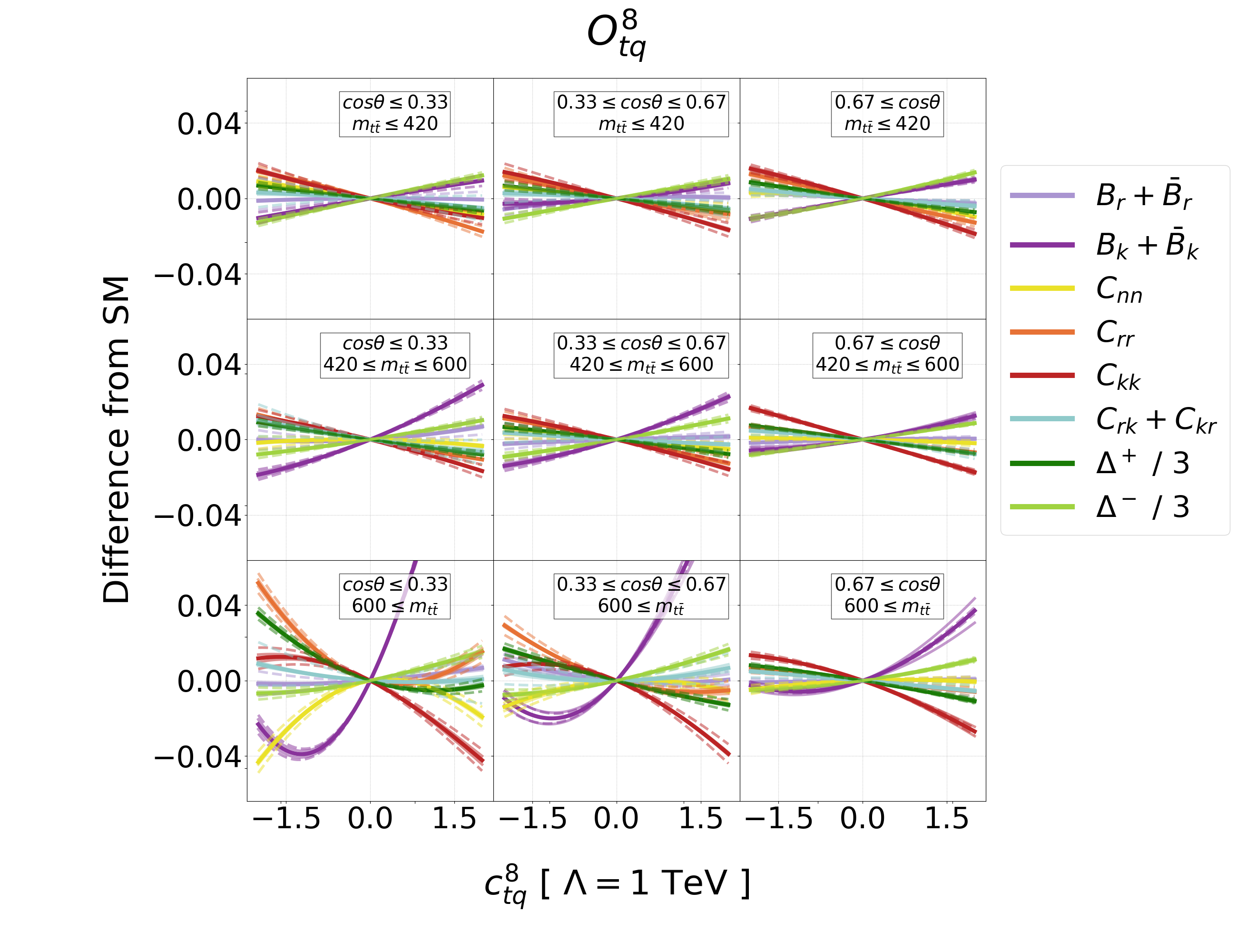
The following Figures 5 - 7, similarly to Figures 1 - 3, show, for selected SMEFT operators, the change at NLO with respect to the SM value for the top spin polarizations Bi+B¯isubscript𝐵𝑖subscript¯𝐵𝑖B_{i}+\bar{B}_{i}, the tt¯𝑡¯𝑡t\bar{t} spin correlations Ciisubscript𝐶𝑖𝑖C_{ii} and Cij+Cjisubscript𝐶𝑖𝑗subscript𝐶𝑗𝑖C_{ij}+C_{ji}, and the entanglement markers Δ±superscriptΔplus-or-minus\Delta^{\pm}, as a function of Wilson coefficients, with tt¯𝑡¯𝑡t\bar{t} phase space binned in the pair invariant mass mtt¯subscript𝑚𝑡¯𝑡m_{t\bar{t}} and in the c.m.f. scattering angle θ𝜃\theta. Figure 4 shows our binning, and the fraction of the total tt¯𝑡¯𝑡t\bar{t} cross-section included in each bin. Even after accounting for detector effects, already after Run 2 of the LHC, all bins contain several million tt¯𝑡¯𝑡t\bar{t} events decaying leptonically.

cosθ1/3𝜃13\cos\theta\leq 1/3 1/3cosθ2/313𝜃231/3\leq\cos\theta\leq 2/3 2/3cosθ23𝜃2/3\leq\cos\theta
mtt¯420GeVsubscript𝑚𝑡¯𝑡420GeVm_{t\bar{t}}\leq 420\,\text{GeV} mtt¯420GeVsubscript𝑚𝑡¯𝑡420GeVm_{t\bar{t}}\leq 420\,\text{GeV} mtt¯420GeVsubscript𝑚𝑡¯𝑡420GeVm_{t\bar{t}}\leq 420\,\text{GeV}
𝝈bin/𝝈=9.0%subscript𝝈bin𝝈percent9.0\bm{\sigma_{\text{bin}}/\sigma=9.0\%} 𝝈bin/𝝈=10.0%subscript𝝈bin𝝈percent10.0\bm{\sigma_{\text{bin}}/\sigma=10.0\%} 𝝈bin/𝝈=12.3%subscript𝝈bin𝝈percent12.3\bm{\sigma_{\text{bin}}/\sigma=12.3\%}
cosθ1/3𝜃13\cos\theta\leq 1/3 1/3cosθ2/313𝜃231/3\leq\cos\theta\leq 2/3 2/3cosθ23𝜃2/3\leq\cos\theta
420GeVmtt¯600GeV420GeVsubscript𝑚𝑡¯𝑡600GeV420\,\text{GeV}\leq m_{t\bar{t}}\leq 600\,\text{GeV} 420GeVmtt¯600GeV420GeVsubscript𝑚𝑡¯𝑡600GeV420\,\text{GeV}\leq m_{t\bar{t}}\leq 600\,\text{GeV} 420GeVmtt¯600GeV420GeVsubscript𝑚𝑡¯𝑡600GeV420\,\text{GeV}\leq m_{t\bar{t}}\leq 600\,\text{GeV}
𝝈bin/𝝈=9.1%subscript𝝈bin𝝈percent9.1\bm{\sigma_{\text{bin}}/\sigma=9.1\%} 𝝈bin/𝝈=12.6%subscript𝝈bin𝝈percent12.6\bm{\sigma_{\text{bin}}/\sigma=12.6\%} 𝝈bin/𝝈=24.6%subscript𝝈bin𝝈percent24.6\bm{\sigma_{\text{bin}}/\sigma=24.6\%}
cosθ1/3𝜃13\cos\theta\leq 1/3 1/3cosθ2/313𝜃231/3\leq\cos\theta\leq 2/3 2/3cosθ23𝜃2/3\leq\cos\theta
600GeVmtt¯600GeVsubscript𝑚𝑡¯𝑡600\,\text{GeV}\leq m_{t\bar{t}} 600GeVmtt¯600GeVsubscript𝑚𝑡¯𝑡600\,\text{GeV}\leq m_{t\bar{t}} 600GeVmtt¯600GeVsubscript𝑚𝑡¯𝑡600\,\text{GeV}\leq m_{t\bar{t}}
𝝈bin/𝝈=2.3%subscript𝝈bin𝝈percent2.3\bm{\sigma_{\text{bin}}/\sigma=2.3\%} 𝝈bin/𝝈=4.0%subscript𝝈bin𝝈percent4.0\bm{\sigma_{\text{bin}}/\sigma=4.0\%} 𝝈bin/𝝈=16.1%subscript𝝈bin𝝈percent16.1\bm{\sigma_{\text{bin}}/\sigma=16.1\%}
Figure 4: Choice of binning of tt¯𝑡¯𝑡t\bar{t} phase-space considered in this work, and fraction of the total cross-section that falls in each bin. Layout reproduces that of our differential plots.
Refer to caption
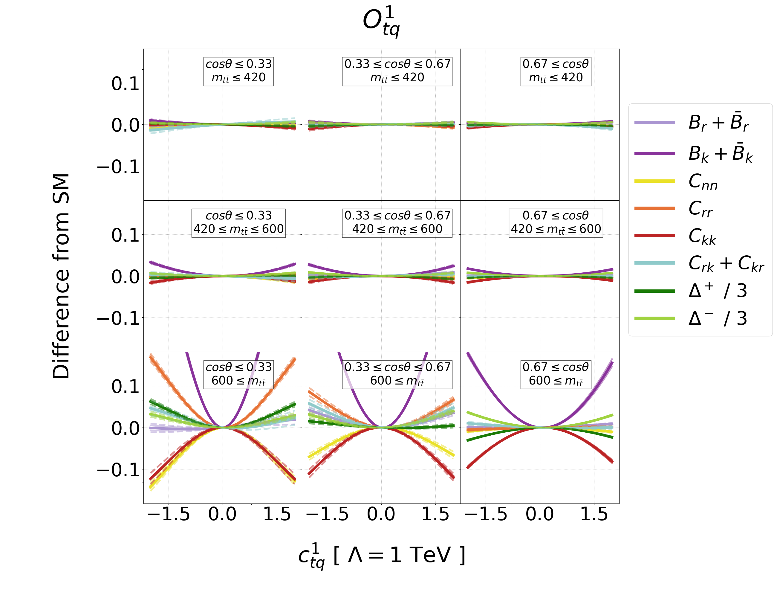
Figure 5: Change at NLO from the SM value for spin observables for the operator 𝒪tGsubscript𝒪𝑡𝐺\mathcal{O}_{tG}. Phase space is divided in the tt¯𝑡¯𝑡t\bar{t} invariant mass along y𝑦y, and in cosθ𝜃\cos\theta along x𝑥x, as indicated by the insets. Continuous lines around each plotted curve indicate scale variation, dashed lines indicate MC uncertainty. Only curves deviating appreciably from zero are shown.
Refer to caption
Figure 6: Results for the operator 𝒪Qq(8,1)superscriptsubscript𝒪𝑄𝑞81\mathcal{O}_{Qq}^{(8,1)}, similar to Figure 5.
Refer to caption
Figure 7: Results for the operators 𝒪Qq(1,1)superscriptsubscript𝒪𝑄𝑞11\mathcal{O}_{Qq}^{(1,1)}, similar to Figure 5.

This Section contains plots for selected SMEFT operators, that have been chosen as their behaviour is representative of the others. Appendix B contains plots for the remaining operators considered in this work. Contrary to the inclusive plots, the doubly-differential plots split the sources of theory uncertainty, with scale variation and Monte Carlo uncertainty shown separately. This is to highlight that, should it become the limiting factor, MC uncertainty is improvable arbitrarily.

We find that spin observables are heavily affected by the presence of new physics, with a rich, and non–trivial structure in tt¯𝑡¯𝑡t\bar{t} phase space. Even a modest cut on the invariant mass, for example our lowest row mtt¯>600GeVsubscript𝑚𝑡¯𝑡600GeVm_{t\bar{t}}>600\,\text{GeV}, can enhance the sensitivity to new physics by a factor of 101010 over an inclusive measurement. On top of the expected growth of deviations from the SM with energy, we find that the tt¯𝑡¯𝑡t\bar{t} kinematical regions that are most sensitive to new physics are those at high-pTsubscript𝑝𝑇p_{T}, already investigated in the context of the observation of quantum entanglement between tops. Aggressive phase space selections in the high-pTsubscript𝑝𝑇p_{T} region will yield increasing gains in sensitivity, but will realistically come with a corresponding worsening of experimental uncertainty, both statistical and systematic.

The variation of the spin correlation observables with different phase space regions is most obvious for the four-fermion operator coefficients. In the Wilson coefficient range we consider, the deviation from the SM predictions varies from the percent level in the low invariant mass region to more than 10% for the high-mass and high-pTsubscript𝑝𝑇p_{T} region for certain operators.

It is also interesting that in several phase-space regions the relation between Wilson coefficients and spin observables is not only departing from the linear regime, but it is also observed to be deviating from a quadratic approximation. This is evident, for instance, for the entanglement marker ΔsuperscriptΔ\Delta^{-} in the high mtt¯subscript𝑚𝑡¯𝑡m_{t\bar{t}} region of the 𝒪tGsubscript𝒪𝑡𝐺\mathcal{O}_{tG} plot, where two saddle points can be seen. Such a rich and non-trivial behaviour highlights the advantage of our full parametrization (3.13) over series expansions.

To conclude this Section, we note that for certain operators, even after enhancing the impact on the observables by focusing on the high-energy regions, the deviation from the SM remains at the 2-3% level in the Wilson coefficient range still allowed by other measurements. For these operators it will be challenging to obtain stringent constraints on the coefficients using spin observables, as this would require extremely precise measurements, probably beyond the reach of present colliders.

6 Constraints on the Wilson coefficients

The early Run 2 top spin polarization and tt¯𝑡¯𝑡t\bar{t} spin correlation measurement from the CMS Collaboration CMS:2019nrx is the only experimental result, as of 2022, where the full spin density matrix is reconstructed. The measurement covers 35.9fb135.9superscriptfb135.9\,\text{fb}^{-1} of integrated luminosity, and is performed inclusively in phase space, which largely washes out the intricate structure of spin observables.

As we do not expect that constraints obtained from CMS:2019nrx will be competitive with the global fit of top data from the LHC Ethier:2021bye , we do not perform a global fit employing the state-of-the-art statistical machinery developed in Ethier:2021bye , but only consider one SMEFT operator at a time, and a χ2superscript𝜒2\chi^{2} parameter estimation. Our fit considers our most accurate SMEFT results, at NLO QCD and quadratic in c/Λ2𝑐superscriptΛ2c/\Lambda^{2}. The most accurate SM predictions available are at NLO QCD + EW Bernreuther:2015yna and NNLO QCD Czakon:2020qbd . Due to the large uncertainty of the experimental measurement, the use of NNLO QCD or NLO QCD + EW SM makes a negligible difference on the final fit results. The numbers we quote in the following use Bernreuther:2015yna as the SM central value. We consider as experimental sources of uncertainty the full statistical and systematic covariance matrices of CMS:2019nrx ; theory uncertainty includes SM scale variation, SMEFT scale variation, and the full statistical covariance matrix of the SMEFT contribution. We assume Gaussian probability density functions for the uncertainties.

The 2σ2𝜎2\,\sigma allowed range for the Wilson coefficient of all SMEFT operators considered in this work are in the first column of Table 4. The range we obtain for ctGsubscript𝑐𝑡𝐺c_{tG} is similar to the one already obtained by the CMS Collaboration in CMS:2019nrx using a SMEFT theory prediction accurate at LO QCD and linear in c/Λ2𝑐superscriptΛ2c/\Lambda^{2}. As noted above, this is due to the nature of the top chromomagnetic moment operator 𝒪tGsubscript𝒪𝑡𝐺\mathcal{O}_{tG}, which leads to a significant interference with LO QCD SM amplitudes. A selection of color-octet four-fermion operators has also been constrained in CMS:2019nrx . While it is true that, after accounting for the different conventions and restricting our results to LO QCD and linear in c/Λ2𝑐superscriptΛ2c/\Lambda^{2}, we are able to obtain similar exclusion ranges, we find that quadratic SMEFT (and, to a lesser extent, higher order QCD) contributions amount to sizable corrections. In our fit we also constrain all seven directions in the four-fermion color-octet parameter space, compared to the six considered in CMS:2019nrx , and constrain the four-fermion color-singlet sector for the first time.

The range obtained from the global fit of LHC data Ethier:2021bye is also reported in Table 4. The bounds we obtain from the CMS inclusive measurement CMS:2019nrx are as expected significantly worse than the results obtained in global analyses of the top sector as these typically involve over a hundred data points constraining these operators. For most four-fermion operators the constraints we obtain are less stringent than the global fit by up to one order of magnitude, whilst for the chromomagnetic operator 𝒪tGsubscript𝒪𝑡𝐺\mathcal{O}_{tG} the bounds are different by a factor of a few.

To explore the potential of spin observables in constraining SMEFT operators in the future, we obtain estimates for a binned measurement using LHC Run 3 data, proceeding as follows. We assume the binning used by experimental collaborations will be the one presented above, 3×3333\times 3 in cosθmtt¯𝜃subscript𝑚𝑡¯𝑡\cos\theta-m_{t\bar{t}}. The experimental statistical covariance is obtained by rescaling the one in CMS:2019nrx to an integrated luminosity of 300fb1300superscriptfb1300\,\text{fb}^{-1} at s=13.6TeV𝑠13.6TeV\sqrt{s}=13.6\,\text{TeV}. We note that in practice this means setting the statistical uncertainty to zero, as the existing measurement is already systematics-dominated. The systematic covariance matrix is obtained by assuming the systematics of the inclusive measurement CMS:2019nrx are replicated in each bin, neglecting bin-to-bin correlations. While it is more than likely that between the early Run 2 measurement CMS:2019nrx and the end of Run 3 significant improvements on the systematic uncertainties will be obtained, moving from an inclusive to a differential measurement will inevitably come with a worsening of the experimental resolution. It is impossible, a priori, to assess precisely either of these two effects. Assigning the early Run 2 systematic uncertainties in each bin of our projected Run 3 measurement is a compromise we consider to be realistic for the near future and conservative in the medium term. We also consider the SM and SMEFT scale variation, as described above, as a source of theory uncertainty. Monte Carlo uncertainty is not considered, as it can be lowered as needed. The bounds we obtain in this way are in the second column of Table 4.

Whilst the bounds obtained from the CMS inclusive measurement CMS:2019nrx are typically approximately an order of magnitude broader than those obtained from the global fit, a binned measurement with LHC Run 3 statistics and present-day systematics would yield bounds competitive or better than those in the global fit. Even though we do not perform a global fit, we advocate that spin observables should be included in future global fits. In particular, entanglement markers such as Δ±superscriptΔplus-or-minus\Delta^{\pm}, being measurable to a significantly greater accuracy than the individual Cijsubscript𝐶𝑖𝑗C_{ij}’s, should also be considered, and may in fact be the observables yielding the best sensitivity. For instance, in CMS:2019nrx , Crrsubscript𝐶𝑟𝑟C_{rr} was measured to a relative accuracy of 46%percent4646\%, Crk+Ckrsubscript𝐶𝑟𝑘subscript𝐶𝑘𝑟C_{rk}+C_{kr} to 31%percent3131\%, while ΔsuperscriptΔ\Delta^{-} was measured to 5%percent55\%.

The expected improvement in the global fit driven by the inclusion of spin/entanglement measurements is a result of two concurring facts. First, the effect of most operators on the cross-sections σSsubscript𝜎𝑆\sigma_{S} are qualitatively different from the effect of the same operators on the total tt¯𝑡¯𝑡t\bar{t} cross-section σ𝜎\sigma. In several cases, the effects on σSsubscript𝜎𝑆\sigma_{S} and σ𝜎\sigma have similar magnitude but opposite sign, so that the resulting shift on the ratio S=σS/σ𝑆subscript𝜎𝑆𝜎S=\sigma_{S}/\sigma is enhanced with respect to the shift of σ𝜎\sigma alone. In other cases, as noted in previous Sections, σSsubscript𝜎𝑆\sigma_{S} is sensitive to particular combinations of Wilson coefficients, e.g. (5.4) and (5.5) for Bk+Bk¯subscript𝐵𝑘¯subscript𝐵𝑘B_{k}+\overline{B_{k}}, that do not appear in σ𝜎\sigma at all. Second, the sheer number of new observables, that in fact probe new, never added before, tt¯𝑡¯𝑡t\bar{t} degrees of freedom, significantly improves the fit quality.

It is not inconceivable that, assuming differential and doubly-differential spin measurements turn out to be experimentally feasible, in the future the bounds for several Wilson coefficients that enter tt¯𝑡¯𝑡t\bar{t} physics will receive significant contributions from spin polarization, spin correlation, and spin entanglement observables.

Operator CMS CMS:2019nrx Run III Projection Current Global Fit
36fb136superscriptfb136\,\text{fb}^{-1} Inclusive 300fb1300superscriptfb1300\,\text{fb}^{-1} Differential
𝒪tGsubscript𝒪𝑡𝐺\mathcal{O}_{tG} [0.18,0.18]0.180.18[-0.18,0.18] [0.03,0.04]0.030.04[-0.03,0.04] [0.00,0.11]0.000.11[0.00,0.11]
𝒪tu8superscriptsubscript𝒪𝑡𝑢8\mathcal{O}_{tu}^{8} [5.8,3.6]5.83.6[-5.8,3.6] [1.0,0.7]1.00.7[-1.0,0.7] [0.9,0.3]0.90.3[-0.9,0.3]
𝒪td8superscriptsubscript𝒪𝑡𝑑8\mathcal{O}_{td}^{8} [7.9,5.2]7.95.2[-7.9,5.2] [1.3,1.0]1.31.0[-1.3,1.0] [1.3,0.6]1.30.6[-1.3,0.6]
𝒪tq8superscriptsubscript𝒪𝑡𝑞8\mathcal{O}_{tq}^{8} [4.2,3.1]4.23.1[-4.2,3.1] [0.7,0.5]0.70.5[-0.7,0.5] [0.5,0.4]0.50.4[-0.5,0.4]
𝒪Qu8superscriptsubscript𝒪𝑄𝑢8\mathcal{O}_{Qu}^{8} [9.4,4.6]9.44.6[-9.4,4.6] [0.7,0.6]0.70.6[-0.7,0.6] [1.0,0.5]1.00.5[-1.0,0.5]
𝒪Qd8superscriptsubscript𝒪𝑄𝑑8\mathcal{O}_{Qd}^{8} [11.7,5.8]11.75.8[-11.7,5.8] [0.9,0.8]0.90.8[-0.9,0.8] [1.6,0.9]1.60.9[-1.6,0.9]
𝒪Qq(1,8)superscriptsubscript𝒪𝑄𝑞18\mathcal{O}_{Qq}^{(1,8)} [5.8,4.6][1.7,2.5]5.84.61.72.5[-5.8,-4.6]\cup[-1.7,2.5] [0.4,0.3]0.40.3[-0.4,0.3] [0.4,0.3]0.40.3[-0.4,0.3]
𝒪Qq(3,8)superscriptsubscript𝒪𝑄𝑞38\mathcal{O}_{Qq}^{(3,8)} [5.0,4.2]5.04.2[-5.0,4.2] [1.1,0.8]1.10.8[-1.1,0.8] [0.5,0.4]0.50.4[-0.5,0.4]
𝒪tu1superscriptsubscript𝒪𝑡𝑢1\mathcal{O}_{tu}^{1} [2.1,2.1]2.12.1[-2.1,2.1] [0.5,0.5]0.50.5[-0.5,0.5] [0.4,0.3]0.40.3[-0.4,0.3]
𝒪td1superscriptsubscript𝒪𝑡𝑑1\mathcal{O}_{td}^{1} [2.7,2.6]2.72.6[-2.7,2.6] [0.6,0.6]0.60.6[-0.6,0.6] [0.4,0.4]0.40.4[-0.4,0.4]
𝒪tq1superscriptsubscript𝒪𝑡𝑞1\mathcal{O}_{tq}^{1} [1.7,1.8]1.71.8[-1.7,1.8] [0.4,0.4]0.40.4[-0.4,0.4] [0.2,0.3]0.20.3[-0.2,0.3]
𝒪Qu1superscriptsubscript𝒪𝑄𝑢1\mathcal{O}_{Qu}^{1} [2.1,2.4]2.12.4[-2.1,2.4] [0.4,0.5]0.40.5[-0.4,0.5] [0.3,0.4]0.30.4[-0.3,0.4]
𝒪Qd1superscriptsubscript𝒪𝑄𝑑1\mathcal{O}_{Qd}^{1} [2.8,3.0]2.83.0[-2.8,3.0] [0.6,0.6]0.60.6[-0.6,0.6] [0.3,0.4]0.30.4[-0.3,0.4]
𝒪Qq(1,1)superscriptsubscript𝒪𝑄𝑞11\mathcal{O}_{Qq}^{(1,1)} [1.8,1.8]1.81.8[-1.8,1.8] [0.4,0.4]0.40.4[-0.4,0.4] [0.3,0.2]0.30.2[-0.3,0.2]
𝒪Qq(3,1)superscriptsubscript𝒪𝑄𝑞31\mathcal{O}_{Qq}^{(3,1)} [1.8,1.8]1.81.8[-1.8,1.8] [0.4,0.4]0.40.4[-0.4,0.4] [0.1,0.2]0.10.2[-0.1,0.2]
Table 4: 2σ2𝜎2\sigma bounds on Wilson coefficients of SMEFT operators considered in this work. The scale ΛΛ\Lambda is set to 1 TeV. First column: bounds from the inclusive early LHC Run 2 experimental measurement CMS:2019nrx . Second column: projected bounds from one binned, LHC Run 3 measurement. Third column: current individual bounds from the global fit of top LHC data Ethier:2021bye .

7 Conclusions

We have presented a numerical simulation of the effect of new physics on top spin polarization, tt¯𝑡¯𝑡t\bar{t} spin correlation, and tt¯𝑡¯𝑡t\bar{t} spin entanglement at the LHC, in the framework of the Standard Model Effective Field Theory. Our simulation is accurate at NLO QCD in the tt¯𝑡¯𝑡t\bar{t} production, and considers both 𝒪(c/Λ2)𝒪𝑐superscriptΛ2\mathcal{O}(c/\Lambda^{2}) and 𝒪(c2/Λ4)𝒪superscript𝑐2superscriptΛ4\mathcal{O}(c^{2}/\Lambda^{4}) effects, which is state of the art. All dimension-6 operators containing top quarks have been considered, with the exception of those highly suppressed by the proton PDF and those only entering in NLO corrections. This amounts to 15 operators in total. We have presented results for the expected deviations from the SM as a function of all Wilson coefficients for all non-CP-violating terms in the tt¯𝑡¯𝑡t\bar{t} density matrix.

We find that the inclusion of NP-squared 𝒪(c2/Λ4)𝒪superscript𝑐2superscriptΛ4\mathcal{O}(c^{2}/\Lambda^{4}) contributions to cross-sections is almost always important for describing the effects of SMEFT operators on all spin observables. This is true not only for color-singlet operators, whose interference with the LO SM QCD amplitude vanishes, but also for the color-octets, in the range of Wilson coefficients still allowed by other measurements. The notable exception is the top chromomagnetic moment operator 𝒪tGsubscript𝒪𝑡𝐺\mathcal{O}_{tG}, for which a LO analysis is found to be adequate. Next-to-leading order QCD corrections, evaluated here for the first time, do not radically change the patterns seen at LO, but the appearance of relatively large K𝐾K-factors on several cross-sections often makes LO scale variation a poor estimate of missing higher orders. As expected, NLO corrections also significantly reduce the uncertainties due to missing higher orders as quantified by scale variations.

We presented results both for an inclusive measurement, and for a doubly-differential measurement in the top pair phase space. Already at the inclusive level, we find that spin observables depend on Wilson coefficients in a largely different way than the total tt¯𝑡¯𝑡t\bar{t} cross-section, thus providing a novel sensitivity to new physics in the top sector. Our second scenario is for a measurement binned in the top pair invariant mass and in the top scattering angle. All spin observables show an intricate structure in phase space. The kinematical region that seems most promising for the detection of NP is the one at large top pTsubscript𝑝𝑇p_{T}, already considered in the context of detection of quantum effects, such as entanglement between the tops’ spin and possible violations of Bell Inequalities.

Only one experimental result is available as of this writing, an early Run 2 measurement from the CMS Collaboration CMS:2019nrx , where the tt¯𝑡¯𝑡t\bar{t} spin density matrix has been fully measured, however without any phase space cuts. No significant deviation from the SM was observed. We argue that this should not be taken as discouraging, as the effects induced by new physics are localized in phase-space, and are washed out by an inclusive measurement.

Using our results and precision SM calculations, we extract bounds for Wilson coefficients from the CMS measurement CMS:2019nrx , and produce a projection for an LHC Run 3 differential measurement. We find that just one doubly-differential measurement of the tt¯𝑡¯𝑡t\bar{t} spin density matrix would yield constraints competitive with the current full global fit to LHC data.

Apart from the prospects of detecting quantum entanglement at the TeV scale Afik:2020onf ; Afik:2022kwm ; Aguilar-Saavedra:2022uye , and possibly observing Bell Inequalities violations Fabbrichesi:2021npl ; Severi:2021cnj , we have shown how the inclusion of spin measurements in the physics program of experimental collaborations would yield a novel and promising road for detecting beyond the SM effects, and provided a systematic and complete framework for these studies.

8 Acknowledgements

We are grateful to Fabio Maltoni and Luca Mantani for comments on the manuscript, and to Rafael Aoude and Olivier Mattelaer for useful discussions. We also thank Ioannis Tsinikos for collaboration at the early stages of this work, and Rikkert Frederix and Timea Vitos for the valuable help. The Authors are supported by the European Union’s Horizon 2020 research and innovation program under the EFT4NP project (grant agreement no. 949451) and by a Royal Society University Research Fellowship through grant URF/R1/201553.

Appendix A Numerical results inclusive in phase space

The following Tables 5 - 12 collect numerical results needed to reproduce our plots in Figures 1 - 3. We present all cross sections at LO and NLO appearing in the numerator and denominator of (3.13) for the spin polarization observables Bi+B¯isubscript𝐵𝑖subscript¯𝐵𝑖B_{i}+\bar{B}_{i}, and the spin correlation observables Ciisubscript𝐶𝑖𝑖C_{ii} and Cij+Cjisubscript𝐶𝑖𝑗subscript𝐶𝑗𝑖C_{ij}+C_{ji}, for all operators we considered. The first quoted uncertainty, in brackets, is Monte Carlo, in units of the least significant digit of the central value. The second one, y+xsubscriptsuperscriptabsent𝑥𝑦{}^{+x}_{-y}, is scale variation333The scale variation we quote on (3.13) is not obtained by propagating the scale variation from each term, but it is extracted by evaluating the full ratio at each scale choice..

SM 𝒪tGsubscript𝒪𝑡𝐺\mathcal{O}_{tG}
Observable Order σ(0)superscript𝜎0\sigma^{(0)} [pb] σ(1)superscript𝜎1\sigma^{(1)} [pb] σ(2)superscript𝜎2\sigma^{(2)} [pb]
σ𝜎\sigma LO 29.12(2)6.49+9.1029.12\scriptstyle{(2)}\,\displaystyle{{}^{+9.10}_{-6.49}} 9.32(7)2.08+2.909.32\scriptstyle{(7)}\,\displaystyle{{}^{+2.90}_{-2.08}} 1.63(1)0.37+0.521.63\scriptstyle{(1)}\,\displaystyle{{}^{+0.52}_{-0.37}}
NLO 36.23(2)3.14+1.7036.23\scriptstyle{(2)}\,\displaystyle{{}^{+1.70}_{-3.14}} 11.50(6)0.97+0.5111.50\scriptstyle{(6)}\,\displaystyle{{}^{+0.51}_{-0.97}} 2.01(1)0.17+0.092.01\scriptstyle{(1)}\,\displaystyle{{}^{+0.09}_{-0.17}}
σBn+B¯nsubscript𝜎subscript𝐵𝑛subscript¯𝐵𝑛\sigma_{\displaystyle B_{n}+\bar{B}_{n}} LO 0.09(5)0.03+0.02-0.09\scriptstyle{(5)}\,\displaystyle{{}^{+0.02}_{-0.03}} 0.01(19)0.00+0.00-0.01\scriptstyle{(19)}\,\displaystyle{{}^{+0.00}_{-0.00}} 0.00(4)0.00+0.00-0.00\scriptstyle{(4)}\,\displaystyle{{}^{+0.00}_{-0.00}}
NLO 0.04(6)0.01+0.00-0.04\scriptstyle{(6)}\,\displaystyle{{}^{+0.00}_{-0.01}} 0.00(24)0.00+0.010.00\scriptstyle{(24)}\,\displaystyle{{}^{+0.01}_{-0.00}} 0.01(5)0.00+0.000.01\scriptstyle{(5)}\,\displaystyle{{}^{+0.00}_{-0.00}}
σBr+B¯rsubscript𝜎subscript𝐵𝑟subscript¯𝐵𝑟\sigma_{\displaystyle B_{r}+\bar{B}_{r}} LO 0.04(6)0.01+0.010.04\scriptstyle{(6)}\,\displaystyle{{}^{+0.01}_{-0.01}} 0.01(23)0.00+0.00-0.01\scriptstyle{(23)}\,\displaystyle{{}^{+0.00}_{-0.00}} 0.00(4)0.00+0.00-0.00\scriptstyle{(4)}\,\displaystyle{{}^{+0.00}_{-0.00}}
NLO 0.03(7)0.02+0.030.03\scriptstyle{(7)}\,\displaystyle{{}^{+0.03}_{-0.02}} 0.01(27)0.01+0.01-0.01\scriptstyle{(27)}\,\displaystyle{{}^{+0.01}_{-0.01}} 0.00(5)0.00+0.00-0.00\scriptstyle{(5)}\,\displaystyle{{}^{+0.00}_{-0.00}}
σBk+B¯ksubscript𝜎subscript𝐵𝑘subscript¯𝐵𝑘\sigma_{\displaystyle B_{k}+\bar{B}_{k}} LO 0.11(6)0.02+0.030.11\scriptstyle{(6)}\,\displaystyle{{}^{+0.03}_{-0.02}} 0.02(23)0.01+0.01-0.02\scriptstyle{(23)}\,\displaystyle{{}^{+0.01}_{-0.01}} 0.01(4)0.00+0.00-0.01\scriptstyle{(4)}\,\displaystyle{{}^{+0.00}_{-0.00}}
NLO 0.04(4)0.02+0.030.04\scriptstyle{(4)}\,\displaystyle{{}^{+0.03}_{-0.02}} 0.03(16)0.01+0.010.03\scriptstyle{(16)}\,\displaystyle{{}^{+0.01}_{-0.01}} 0.00(3)0.00+0.000.00\scriptstyle{(3)}\,\displaystyle{{}^{+0.00}_{-0.00}}
σCnnsubscript𝜎subscript𝐶𝑛𝑛\sigma_{\displaystyle C_{nn}} LO 9.63(8)2.13+2.969.63\scriptstyle{(8)}\,\displaystyle{{}^{+2.96}_{-2.13}} 6.68(31)1.52+2.136.68\scriptstyle{(31)}\,\displaystyle{{}^{+2.13}_{-1.52}} 0.40(5)0.09+0.130.40\scriptstyle{(5)}\,\displaystyle{{}^{+0.13}_{-0.09}}
NLO 11.27(6)0.80+0.4311.27\scriptstyle{(6)}\,\displaystyle{{}^{+0.43}_{-0.80}} 8.30(27)0.72+0.428.30\scriptstyle{(27)}\,\displaystyle{{}^{+0.42}_{-0.72}} 0.56(5)0.06+0.050.56\scriptstyle{(5)}\,\displaystyle{{}^{+0.05}_{-0.06}}
σCrrsubscript𝜎subscript𝐶𝑟𝑟\sigma_{\displaystyle C_{rr}} LO 0.19(8)0.13+0.190.19\scriptstyle{(8)}\,\displaystyle{{}^{+0.19}_{-0.13}} 4.37(31)1.02+1.444.37\scriptstyle{(31)}\,\displaystyle{{}^{+1.44}_{-1.02}} 0.65(5)0.15+0.210.65\scriptstyle{(5)}\,\displaystyle{{}^{+0.21}_{-0.15}}
NLO 1.66(6)0.45+0.651.66\scriptstyle{(6)}\,\displaystyle{{}^{+0.65}_{-0.45}} 5.75(26)0.57+0.375.75\scriptstyle{(26)}\,\displaystyle{{}^{+0.37}_{-0.57}} 0.81(5)0.07+0.040.81\scriptstyle{(5)}\,\displaystyle{{}^{+0.04}_{-0.07}}
σCkksubscript𝜎subscript𝐶𝑘𝑘\sigma_{\displaystyle C_{kk}} LO 9.42(7)2.22+3.129.42\scriptstyle{(7)}\,\displaystyle{{}^{+3.12}_{-2.22}} 4.60(30)1.05+1.474.60\scriptstyle{(30)}\,\displaystyle{{}^{+1.47}_{-1.05}} 0.97(5)0.22+0.310.97\scriptstyle{(5)}\,\displaystyle{{}^{+0.31}_{-0.22}}
NLO 11.83(6)1.03+0.6811.83\scriptstyle{(6)}\,\displaystyle{{}^{+0.68}_{-1.03}} 5.66(24)0.47+0.295.66\scriptstyle{(24)}\,\displaystyle{{}^{+0.29}_{-0.47}} 1.17(5)0.10+0.051.17\scriptstyle{(5)}\,\displaystyle{{}^{+0.05}_{-0.10}}
σCrk+Ckrsubscript𝜎subscript𝐶𝑟𝑘subscript𝐶𝑘𝑟\sigma_{\displaystyle C_{rk}+C_{kr}} LO 6.81(9)2.01+1.45-6.81\scriptstyle{(9)}\,\displaystyle{{}^{+1.45}_{-2.01}} 0.65(36)0.15+0.11-0.65\scriptstyle{(36)}\,\displaystyle{{}^{+0.11}_{-0.15}} 0.03(6)0.01+0.01-0.03\scriptstyle{(6)}\,\displaystyle{{}^{+0.01}_{-0.01}}
NLO 7.36(11)0.13+0.44-7.36\scriptstyle{(11)}\,\displaystyle{{}^{+0.44}_{-0.13}} 1.07(46)0.18+0.14-1.07\scriptstyle{(46)}\,\displaystyle{{}^{+0.14}_{-0.18}} 0.04(9)0.00+0.00-0.04\scriptstyle{(9)}\,\displaystyle{{}^{+0.00}_{-0.00}}
σCnr+Crnsubscript𝜎subscript𝐶𝑛𝑟subscript𝐶𝑟𝑛\sigma_{\displaystyle C_{nr}+C_{rn}} LO 0.06(8)0.02+0.01-0.06\scriptstyle{(8)}\,\displaystyle{{}^{+0.01}_{-0.02}} 0.02(33)0.01+0.01-0.02\scriptstyle{(33)}\,\displaystyle{{}^{+0.01}_{-0.01}} 0.00(6)0.00+0.00-0.00\scriptstyle{(6)}\,\displaystyle{{}^{+0.00}_{-0.00}}
NLO 0.03(10)0.03+0.04-0.03\scriptstyle{(10)}\,\displaystyle{{}^{+0.04}_{-0.03}} 0.03(41)0.02+0.01-0.03\scriptstyle{(41)}\,\displaystyle{{}^{+0.01}_{-0.02}} 0.01(8)0.00+0.00-0.01\scriptstyle{(8)}\,\displaystyle{{}^{+0.00}_{-0.00}}
σCnk+Cknsubscript𝜎subscript𝐶𝑛𝑘subscript𝐶𝑘𝑛\sigma_{\displaystyle C_{nk}+C_{kn}} LO 0.11(10)0.03+0.040.11\scriptstyle{(10)}\,\displaystyle{{}^{+0.04}_{-0.03}} 0.04(40)0.02+0.01-0.04\scriptstyle{(40)}\,\displaystyle{{}^{+0.01}_{-0.02}} 0.01(7)0.00+0.00-0.01\scriptstyle{(7)}\,\displaystyle{{}^{+0.00}_{-0.00}}
NLO 0.16(10)0.04+0.050.16\scriptstyle{(10)}\,\displaystyle{{}^{+0.05}_{-0.04}} 0.01(44)0.01+0.030.01\scriptstyle{(44)}\,\displaystyle{{}^{+0.03}_{-0.01}} 0.00(9)0.00+0.000.00\scriptstyle{(9)}\,\displaystyle{{}^{+0.00}_{-0.00}}
Table 5: Numerical results for the Standard Model and for the operator 𝒪tGsubscript𝒪𝑡𝐺\mathcal{O}_{tG}.
𝒪Qq(8,3)superscriptsubscript𝒪𝑄𝑞83\mathcal{O}_{Qq}^{(8,3)} 𝒪Qq(1,3)superscriptsubscript𝒪𝑄𝑞13\mathcal{O}_{Qq}^{(1,3)}
Observable Order σ(1)superscript𝜎1\sigma^{(1)} [pb] σ(2)superscript𝜎2\sigma^{(2)} [pb] σ(1)superscript𝜎1\sigma^{(1)} [pb] σ(2)superscript𝜎2\sigma^{(2)} [pb]
σ𝜎\sigma LO 0.073(2)0.007+0.0080.073\scriptstyle{(2)}\,\displaystyle{{}^{+0.008}_{-0.007}} 0.075(0)0.004+0.0040.075\scriptstyle{(0)}\,\displaystyle{{}^{+0.004}_{-0.004}} 0.006(4)0.001+0.0020.006\scriptstyle{(4)}\,\displaystyle{{}^{+0.002}_{-0.001}} 0.334(1)0.017+0.0190.334\scriptstyle{(1)}\,\displaystyle{{}^{+0.019}_{-0.017}}
NLO 0.059(3)0.005+0.0020.059\scriptstyle{(3)}\,\displaystyle{{}^{+0.002}_{-0.005}} 0.072(1)0.001+0.0020.072\scriptstyle{(1)}\,\displaystyle{{}^{+0.002}_{-0.001}} 0.002(3)0.000+0.001-0.002\scriptstyle{(3)}\,\displaystyle{{}^{+0.001}_{-0.000}} 0.476(1)0.022+0.0250.476\scriptstyle{(1)}\,\displaystyle{{}^{+0.025}_{-0.022}}
σBn+B¯nsubscript𝜎subscript𝐵𝑛subscript¯𝐵𝑛\sigma_{\displaystyle B_{n}+\bar{B}_{n}} LO 0.002(7)0.000+0.0000.002\scriptstyle{(7)}\,\displaystyle{{}^{+0.000}_{-0.000}} 0.003(2)0.001+0.001-0.003\scriptstyle{(2)}\,\displaystyle{{}^{+0.001}_{-0.001}} 0.002(12)0.001+0.002-0.002\scriptstyle{(12)}\,\displaystyle{{}^{+0.002}_{-0.001}} 0.006(3)0.001+0.001-0.006\scriptstyle{(3)}\,\displaystyle{{}^{+0.001}_{-0.001}}
NLO 0.009(10)0.007+0.004-0.009\scriptstyle{(10)}\,\displaystyle{{}^{+0.004}_{-0.007}} 0.000(2)0.000+0.0010.000\scriptstyle{(2)}\,\displaystyle{{}^{+0.001}_{-0.000}} 0.022(13)0.006+0.0100.022\scriptstyle{(13)}\,\displaystyle{{}^{+0.010}_{-0.006}} 0.003(3)0.001+0.0010.003\scriptstyle{(3)}\,\displaystyle{{}^{+0.001}_{-0.001}}
σBr+B¯rsubscript𝜎subscript𝐵𝑟subscript¯𝐵𝑟\sigma_{\displaystyle B_{r}+\bar{B}_{r}} LO 0.008(7)0.001+0.001-0.008\scriptstyle{(7)}\,\displaystyle{{}^{+0.001}_{-0.001}} 0.011(2)0.000+0.001-0.011\scriptstyle{(2)}\,\displaystyle{{}^{+0.001}_{-0.000}} 0.002(15)0.005+0.003-0.002\scriptstyle{(15)}\,\displaystyle{{}^{+0.003}_{-0.005}} 0.050(3)0.003+0.003-0.050\scriptstyle{(3)}\,\displaystyle{{}^{+0.003}_{-0.003}}
NLO 0.011(11)0.003+0.003-0.011\scriptstyle{(11)}\,\displaystyle{{}^{+0.003}_{-0.003}} 0.005(2)0.001+0.001-0.005\scriptstyle{(2)}\,\displaystyle{{}^{+0.001}_{-0.001}} 0.005(14)0.004+0.006-0.005\scriptstyle{(14)}\,\displaystyle{{}^{+0.006}_{-0.004}} 0.059(3)0.002+0.001-0.059\scriptstyle{(3)}\,\displaystyle{{}^{+0.001}_{-0.002}}
σBk+B¯ksubscript𝜎subscript𝐵𝑘subscript¯𝐵𝑘\sigma_{\displaystyle B_{k}+\bar{B}_{k}} LO 0.079(10)0.011+0.008-0.079\scriptstyle{(10)}\,\displaystyle{{}^{+0.008}_{-0.011}} 0.133(3)0.013+0.011-0.133\scriptstyle{(3)}\,\displaystyle{{}^{+0.011}_{-0.013}} 0.036(23)0.008+0.0070.036\scriptstyle{(23)}\,\displaystyle{{}^{+0.007}_{-0.008}} 0.584(5)0.043+0.038-0.584\scriptstyle{(5)}\,\displaystyle{{}^{+0.038}_{-0.043}}
NLO 0.083(7)0.001+0.004-0.083\scriptstyle{(7)}\,\displaystyle{{}^{+0.004}_{-0.001}} 0.118(2)0.001+0.002-0.118\scriptstyle{(2)}\,\displaystyle{{}^{+0.002}_{-0.001}} 0.004(16)0.004+0.007-0.004\scriptstyle{(16)}\,\displaystyle{{}^{+0.007}_{-0.004}} 0.761(4)0.034+0.031-0.761\scriptstyle{(4)}\,\displaystyle{{}^{+0.031}_{-0.034}}
σCnnsubscript𝜎subscript𝐶𝑛𝑛\sigma_{\displaystyle C_{nn}} LO 0.019(10)0.001+0.0020.019\scriptstyle{(10)}\,\displaystyle{{}^{+0.002}_{-0.001}} 0.002(3)0.000+0.0000.002\scriptstyle{(3)}\,\displaystyle{{}^{+0.000}_{-0.000}} 0.011(14)0.001+0.0010.011\scriptstyle{(14)}\,\displaystyle{{}^{+0.001}_{-0.001}} 0.006(3)0.002+0.002-0.006\scriptstyle{(3)}\,\displaystyle{{}^{+0.002}_{-0.002}}
NLO 0.002(10)0.015+0.008-0.002\scriptstyle{(10)}\,\displaystyle{{}^{+0.008}_{-0.015}} 0.004(2)0.002+0.001-0.004\scriptstyle{(2)}\,\displaystyle{{}^{+0.001}_{-0.002}} 0.006(13)0.003+0.0020.006\scriptstyle{(13)}\,\displaystyle{{}^{+0.002}_{-0.003}} 0.006(3)0.001+0.0010.006\scriptstyle{(3)}\,\displaystyle{{}^{+0.001}_{-0.001}}
σCrrsubscript𝜎subscript𝐶𝑟𝑟\sigma_{\displaystyle C_{rr}} LO 0.031(11)0.003+0.003-0.031\scriptstyle{(11)}\,\displaystyle{{}^{+0.003}_{-0.003}} 0.003(3)0.001+0.002-0.003\scriptstyle{(3)}\,\displaystyle{{}^{+0.002}_{-0.001}} 0.001(14)0.001+0.001-0.001\scriptstyle{(14)}\,\displaystyle{{}^{+0.001}_{-0.001}} 0.029(3)0.001+0.002-0.029\scriptstyle{(3)}\,\displaystyle{{}^{+0.002}_{-0.001}}
NLO 0.027(10)0.005+0.008-0.027\scriptstyle{(10)}\,\displaystyle{{}^{+0.008}_{-0.005}} 0.004(2)0.001+0.000-0.004\scriptstyle{(2)}\,\displaystyle{{}^{+0.000}_{-0.001}} 0.010(13)0.006+0.003-0.010\scriptstyle{(13)}\,\displaystyle{{}^{+0.003}_{-0.006}} 0.040(3)0.002+0.001-0.040\scriptstyle{(3)}\,\displaystyle{{}^{+0.001}_{-0.002}}
σCkksubscript𝜎subscript𝐶𝑘𝑘\sigma_{\displaystyle C_{kk}} LO 0.036(12)0.005+0.004-0.036\scriptstyle{(12)}\,\displaystyle{{}^{+0.004}_{-0.005}} 0.055(3)0.003+0.003-0.055\scriptstyle{(3)}\,\displaystyle{{}^{+0.003}_{-0.003}} 0.085(34)0.004+0.0050.085\scriptstyle{(34)}\,\displaystyle{{}^{+0.005}_{-0.004}} 0.246(8)0.015+0.013-0.246\scriptstyle{(8)}\,\displaystyle{{}^{+0.013}_{-0.015}}
NLO 0.080(10)0.017+0.012-0.080\scriptstyle{(10)}\,\displaystyle{{}^{+0.012}_{-0.017}} 0.041(2)0.001+0.002-0.041\scriptstyle{(2)}\,\displaystyle{{}^{+0.002}_{-0.001}} 0.002(22)0.007+0.015-0.002\scriptstyle{(22)}\,\displaystyle{{}^{+0.015}_{-0.007}} 0.294(5)0.008+0.008-0.294\scriptstyle{(5)}\,\displaystyle{{}^{+0.008}_{-0.008}}
σCrk+Ckrsubscript𝜎subscript𝐶𝑟𝑘subscript𝐶𝑘𝑟\sigma_{\displaystyle C_{rk}+C_{kr}} LO 0.001(15)0.004+0.0070.001\scriptstyle{(15)}\,\displaystyle{{}^{+0.007}_{-0.004}} 0.006(4)0.002+0.002-0.006\scriptstyle{(4)}\,\displaystyle{{}^{+0.002}_{-0.002}} 0.052(23)0.008+0.0110.052\scriptstyle{(23)}\,\displaystyle{{}^{+0.011}_{-0.008}} 0.059(5)0.002+0.003-0.059\scriptstyle{(5)}\,\displaystyle{{}^{+0.003}_{-0.002}}
NLO 0.005(18)0.010+0.020-0.005\scriptstyle{(18)}\,\displaystyle{{}^{+0.020}_{-0.010}} 0.001(4)0.002+0.0020.001\scriptstyle{(4)}\,\displaystyle{{}^{+0.002}_{-0.002}} 0.015(25)0.013+0.007-0.015\scriptstyle{(25)}\,\displaystyle{{}^{+0.007}_{-0.013}} 0.076(6)0.008+0.005-0.076\scriptstyle{(6)}\,\displaystyle{{}^{+0.005}_{-0.008}}
σCnr+Crnsubscript𝜎subscript𝐶𝑛𝑟subscript𝐶𝑟𝑛\sigma_{\displaystyle C_{nr}+C_{rn}} LO 0.006(13)0.001+0.0020.006\scriptstyle{(13)}\,\displaystyle{{}^{+0.002}_{-0.001}} 0.005(3)0.001+0.0020.005\scriptstyle{(3)}\,\displaystyle{{}^{+0.002}_{-0.001}} 0.009(18)0.002+0.001-0.009\scriptstyle{(18)}\,\displaystyle{{}^{+0.001}_{-0.002}} 0.003(4)0.001+0.0010.003\scriptstyle{(4)}\,\displaystyle{{}^{+0.001}_{-0.001}}
NLO 0.013(16)0.007+0.004-0.013\scriptstyle{(16)}\,\displaystyle{{}^{+0.004}_{-0.007}} 0.001(4)0.000+0.0000.001\scriptstyle{(4)}\,\displaystyle{{}^{+0.000}_{-0.000}} 0.013(22)0.004+0.0090.013\scriptstyle{(22)}\,\displaystyle{{}^{+0.009}_{-0.004}} 0.004(5)0.002+0.0030.004\scriptstyle{(5)}\,\displaystyle{{}^{+0.003}_{-0.002}}
σCnk+Cknsubscript𝜎subscript𝐶𝑛𝑘subscript𝐶𝑘𝑛\sigma_{\displaystyle C_{nk}+C_{kn}} LO 0.008(14)0.002+0.002-0.008\scriptstyle{(14)}\,\displaystyle{{}^{+0.002}_{-0.002}} 0.002(4)0.000+0.000-0.002\scriptstyle{(4)}\,\displaystyle{{}^{+0.000}_{-0.000}} 0.011(20)0.004+0.003-0.011\scriptstyle{(20)}\,\displaystyle{{}^{+0.003}_{-0.004}} 0.003(5)0.000+0.000-0.003\scriptstyle{(5)}\,\displaystyle{{}^{+0.000}_{-0.000}}
NLO 0.009(18)0.013+0.007-0.009\scriptstyle{(18)}\,\displaystyle{{}^{+0.007}_{-0.013}} 0.002(4)0.001+0.001-0.002\scriptstyle{(4)}\,\displaystyle{{}^{+0.001}_{-0.001}} 0.026(23)0.009+0.0140.026\scriptstyle{(23)}\,\displaystyle{{}^{+0.014}_{-0.009}} 0.004(5)0.002+0.001-0.004\scriptstyle{(5)}\,\displaystyle{{}^{+0.001}_{-0.002}}
Table 6: Numerical results for the operators 𝒪Qq(8,3)superscriptsubscript𝒪𝑄𝑞83\mathcal{O}_{Qq}^{(8,3)} (left) and 𝒪Qq(1,3)superscriptsubscript𝒪𝑄𝑞13\mathcal{O}_{Qq}^{(1,3)} (right).
𝒪Qq(8,1)superscriptsubscript𝒪𝑄𝑞81\mathcal{O}_{Qq}^{(8,1)} 𝒪Qq(1,1)superscriptsubscript𝒪𝑄𝑞11\mathcal{O}_{Qq}^{(1,1)}
Observable Order σ(1)superscript𝜎1\sigma^{(1)} [pb] σ(2)superscript𝜎2\sigma^{(2)} [pb] σ(1)superscript𝜎1\sigma^{(1)} [pb] σ(2)superscript𝜎2\sigma^{(2)} [pb]
σ𝜎\sigma LO 0.385(2)0.039+0.0460.385\scriptstyle{(2)}\,\displaystyle{{}^{+0.046}_{-0.039}} 0.075(0)0.004+0.0040.075\scriptstyle{(0)}\,\displaystyle{{}^{+0.004}_{-0.004}} 0.002(2)0.000+0.000-0.002\scriptstyle{(2)}\,\displaystyle{{}^{+0.000}_{-0.000}} 0.335(1)0.017+0.0190.335\scriptstyle{(1)}\,\displaystyle{{}^{+0.019}_{-0.017}}
NLO 0.345(3)0.013+0.0030.345\scriptstyle{(3)}\,\displaystyle{{}^{+0.003}_{-0.013}} 0.078(1)0.001+0.0020.078\scriptstyle{(1)}\,\displaystyle{{}^{+0.002}_{-0.001}} 0.019(3)0.006+0.004-0.019\scriptstyle{(3)}\,\displaystyle{{}^{+0.004}_{-0.006}} 0.478(1)0.022+0.0260.478\scriptstyle{(1)}\,\displaystyle{{}^{+0.026}_{-0.022}}
σBn+B¯nsubscript𝜎subscript𝐵𝑛subscript¯𝐵𝑛\sigma_{\displaystyle B_{n}+\bar{B}_{n}} LO 0.013(7)0.003+0.002-0.013\scriptstyle{(7)}\,\displaystyle{{}^{+0.002}_{-0.003}} 0.001(2)0.000+0.0010.001\scriptstyle{(2)}\,\displaystyle{{}^{+0.001}_{-0.000}} 0.006(10)0.001+0.001-0.006\scriptstyle{(10)}\,\displaystyle{{}^{+0.001}_{-0.001}} 0.001(2)0.000+0.0000.001\scriptstyle{(2)}\,\displaystyle{{}^{+0.000}_{-0.000}}
NLO 0.005(10)0.001+0.0030.005\scriptstyle{(10)}\,\displaystyle{{}^{+0.003}_{-0.001}} 0.001(2)0.001+0.0010.001\scriptstyle{(2)}\,\displaystyle{{}^{+0.001}_{-0.001}} 0.005(12)0.005+0.003-0.005\scriptstyle{(12)}\,\displaystyle{{}^{+0.003}_{-0.005}} 0.002(3)0.002+0.001-0.002\scriptstyle{(3)}\,\displaystyle{{}^{+0.001}_{-0.002}}
σBr+B¯rsubscript𝜎subscript𝐵𝑟subscript¯𝐵𝑟\sigma_{\displaystyle B_{r}+\bar{B}_{r}} LO 0.062(9)0.005+0.004-0.062\scriptstyle{(9)}\,\displaystyle{{}^{+0.004}_{-0.005}} 0.012(2)0.001+0.001-0.012\scriptstyle{(2)}\,\displaystyle{{}^{+0.001}_{-0.001}} 0.009(11)0.002+0.0040.009\scriptstyle{(11)}\,\displaystyle{{}^{+0.004}_{-0.002}} 0.054(3)0.002+0.002-0.054\scriptstyle{(3)}\,\displaystyle{{}^{+0.002}_{-0.002}}
NLO 0.074(11)0.004+0.004-0.074\scriptstyle{(11)}\,\displaystyle{{}^{+0.004}_{-0.004}} 0.006(3)0.001+0.002-0.006\scriptstyle{(3)}\,\displaystyle{{}^{+0.002}_{-0.001}} 0.031(13)0.006+0.0080.031\scriptstyle{(13)}\,\displaystyle{{}^{+0.008}_{-0.006}} 0.055(3)0.001+0.001-0.055\scriptstyle{(3)}\,\displaystyle{{}^{+0.001}_{-0.001}}
σBk+B¯ksubscript𝜎subscript𝐵𝑘subscript¯𝐵𝑘\sigma_{\displaystyle B_{k}+\bar{B}_{k}} LO 0.441(10)0.068+0.054-0.441\scriptstyle{(10)}\,\displaystyle{{}^{+0.054}_{-0.068}} 0.123(3)0.011+0.009-0.123\scriptstyle{(3)}\,\displaystyle{{}^{+0.009}_{-0.011}} 0.004(28)0.001+0.000-0.004\scriptstyle{(28)}\,\displaystyle{{}^{+0.000}_{-0.001}} 0.557(7)0.040+0.035-0.557\scriptstyle{(7)}\,\displaystyle{{}^{+0.035}_{-0.040}}
NLO 0.469(7)0.003+0.014-0.469\scriptstyle{(7)}\,\displaystyle{{}^{+0.014}_{-0.003}} 0.129(2)0.003+0.003-0.129\scriptstyle{(2)}\,\displaystyle{{}^{+0.003}_{-0.003}} 0.044(14)0.015+0.011-0.044\scriptstyle{(14)}\,\displaystyle{{}^{+0.011}_{-0.015}} 0.767(4)0.035+0.032-0.767\scriptstyle{(4)}\,\displaystyle{{}^{+0.032}_{-0.035}}
σCnnsubscript𝜎subscript𝐶𝑛𝑛\sigma_{\displaystyle C_{nn}} LO 0.089(10)0.009+0.0100.089\scriptstyle{(10)}\,\displaystyle{{}^{+0.010}_{-0.009}} 0.002(3)0.001+0.0000.002\scriptstyle{(3)}\,\displaystyle{{}^{+0.000}_{-0.001}} 0.004(13)0.002+0.0030.004\scriptstyle{(13)}\,\displaystyle{{}^{+0.003}_{-0.002}} 0.002(3)0.002+0.001-0.002\scriptstyle{(3)}\,\displaystyle{{}^{+0.001}_{-0.002}}
NLO 0.073(9)0.013+0.0070.073\scriptstyle{(9)}\,\displaystyle{{}^{+0.007}_{-0.013}} 0.003(2)0.003+0.002-0.003\scriptstyle{(2)}\,\displaystyle{{}^{+0.002}_{-0.003}} 0.030(13)0.010+0.007-0.030\scriptstyle{(13)}\,\displaystyle{{}^{+0.007}_{-0.010}} 0.004(3)0.002+0.0010.004\scriptstyle{(3)}\,\displaystyle{{}^{+0.001}_{-0.002}}
σCrrsubscript𝜎subscript𝐶𝑟𝑟\sigma_{\displaystyle C_{rr}} LO 0.201(10)0.022+0.019-0.201\scriptstyle{(10)}\,\displaystyle{{}^{+0.019}_{-0.022}} 0.003(3)0.001+0.002-0.003\scriptstyle{(3)}\,\displaystyle{{}^{+0.002}_{-0.001}} 0.019(14)0.004+0.0060.019\scriptstyle{(14)}\,\displaystyle{{}^{+0.006}_{-0.004}} 0.026(4)0.002+0.003-0.026\scriptstyle{(4)}\,\displaystyle{{}^{+0.003}_{-0.002}}
NLO 0.206(11)0.001+0.003-0.206\scriptstyle{(11)}\,\displaystyle{{}^{+0.003}_{-0.001}} 0.004(3)0.001+0.000-0.004\scriptstyle{(3)}\,\displaystyle{{}^{+0.000}_{-0.001}} 0.017(13)0.006+0.0100.017\scriptstyle{(13)}\,\displaystyle{{}^{+0.010}_{-0.006}} 0.032(3)0.002+0.001-0.032\scriptstyle{(3)}\,\displaystyle{{}^{+0.001}_{-0.002}}
σCkksubscript𝜎subscript𝐶𝑘𝑘\sigma_{\displaystyle C_{kk}} LO 0.202(10)0.022+0.020-0.202\scriptstyle{(10)}\,\displaystyle{{}^{+0.020}_{-0.022}} 0.047(3)0.003+0.003-0.047\scriptstyle{(3)}\,\displaystyle{{}^{+0.003}_{-0.003}} 0.004(40)0.001+0.0010.004\scriptstyle{(40)}\,\displaystyle{{}^{+0.001}_{-0.001}} 0.219(10)0.013+0.012-0.219\scriptstyle{(10)}\,\displaystyle{{}^{+0.012}_{-0.013}}
NLO 0.286(11)0.030+0.022-0.286\scriptstyle{(11)}\,\displaystyle{{}^{+0.022}_{-0.030}} 0.047(3)0.002+0.001-0.047\scriptstyle{(3)}\,\displaystyle{{}^{+0.001}_{-0.002}} 0.026(18)0.015+0.010-0.026\scriptstyle{(18)}\,\displaystyle{{}^{+0.010}_{-0.015}} 0.305(5)0.012+0.010-0.305\scriptstyle{(5)}\,\displaystyle{{}^{+0.010}_{-0.012}}
σCrk+Ckrsubscript𝜎subscript𝐶𝑟𝑘subscript𝐶𝑘𝑟\sigma_{\displaystyle C_{rk}+C_{kr}} LO 0.194(14)0.028+0.022-0.194\scriptstyle{(14)}\,\displaystyle{{}^{+0.022}_{-0.028}} 0.011(4)0.001+0.001-0.011\scriptstyle{(4)}\,\displaystyle{{}^{+0.001}_{-0.001}} 0.007(20)0.002+0.0030.007\scriptstyle{(20)}\,\displaystyle{{}^{+0.003}_{-0.002}} 0.046(5)0.005+0.005-0.046\scriptstyle{(5)}\,\displaystyle{{}^{+0.005}_{-0.005}}
NLO 0.167(19)0.005+0.009-0.167\scriptstyle{(19)}\,\displaystyle{{}^{+0.009}_{-0.005}} 0.002(5)0.002+0.003-0.002\scriptstyle{(5)}\,\displaystyle{{}^{+0.003}_{-0.002}} 0.040(23)0.012+0.0200.040\scriptstyle{(23)}\,\displaystyle{{}^{+0.020}_{-0.012}} 0.065(6)0.003+0.002-0.065\scriptstyle{(6)}\,\displaystyle{{}^{+0.002}_{-0.003}}
σCnr+Crnsubscript𝜎subscript𝐶𝑛𝑟subscript𝐶𝑟𝑛\sigma_{\displaystyle C_{nr}+C_{rn}} LO 0.024(14)0.005+0.0070.024\scriptstyle{(14)}\,\displaystyle{{}^{+0.007}_{-0.005}} 0.002(4)0.001+0.001-0.002\scriptstyle{(4)}\,\displaystyle{{}^{+0.001}_{-0.001}} 0.025(19)0.006+0.004-0.025\scriptstyle{(19)}\,\displaystyle{{}^{+0.004}_{-0.006}} 0.003(5)0.000+0.0000.003\scriptstyle{(5)}\,\displaystyle{{}^{+0.000}_{-0.000}}
NLO 0.012(15)0.003+0.002-0.012\scriptstyle{(15)}\,\displaystyle{{}^{+0.002}_{-0.003}} 0.001(4)0.001+0.001-0.001\scriptstyle{(4)}\,\displaystyle{{}^{+0.001}_{-0.001}} 0.012(20)0.006+0.0090.012\scriptstyle{(20)}\,\displaystyle{{}^{+0.009}_{-0.006}} 0.005(5)0.001+0.001-0.005\scriptstyle{(5)}\,\displaystyle{{}^{+0.001}_{-0.001}}
σCnk+Cknsubscript𝜎subscript𝐶𝑛𝑘subscript𝐶𝑘𝑛\sigma_{\displaystyle C_{nk}+C_{kn}} LO 0.002(13)0.001+0.0020.002\scriptstyle{(13)}\,\displaystyle{{}^{+0.002}_{-0.001}} 0.001(3)0.000+0.0000.001\scriptstyle{(3)}\,\displaystyle{{}^{+0.000}_{-0.000}} 0.010(16)0.003+0.002-0.010\scriptstyle{(16)}\,\displaystyle{{}^{+0.002}_{-0.003}} 0.009(4)0.002+0.0020.009\scriptstyle{(4)}\,\displaystyle{{}^{+0.002}_{-0.002}}
NLO 0.005(20)0.005+0.0100.005\scriptstyle{(20)}\,\displaystyle{{}^{+0.010}_{-0.005}} 0.001(5)0.002+0.001-0.001\scriptstyle{(5)}\,\displaystyle{{}^{+0.001}_{-0.002}} 0.001(21)0.013+0.008-0.001\scriptstyle{(21)}\,\displaystyle{{}^{+0.008}_{-0.013}} 0.003(6)0.000+0.0010.003\scriptstyle{(6)}\,\displaystyle{{}^{+0.001}_{-0.000}}
Table 7: Numerical results for the operators 𝒪Qq(8,1)superscriptsubscript𝒪𝑄𝑞81\mathcal{O}_{Qq}^{(8,1)} (left) and 𝒪Qq(1,1)superscriptsubscript𝒪𝑄𝑞11\mathcal{O}_{Qq}^{(1,1)} (right).
𝒪Qu8superscriptsubscript𝒪𝑄𝑢8\mathcal{O}_{Qu}^{8} 𝒪Qu1superscriptsubscript𝒪𝑄𝑢1\mathcal{O}_{Qu}^{1}
Observable Order σ(1)superscript𝜎1\sigma^{(1)} [pb] σ(2)superscript𝜎2\sigma^{(2)} [pb] σ(1)superscript𝜎1\sigma^{(1)} [pb] σ(2)superscript𝜎2\sigma^{(2)} [pb]
σ𝜎\sigma LO 0.230(2)0.023+0.0270.230\scriptstyle{(2)}\,\displaystyle{{}^{+0.027}_{-0.023}} 0.046(0)0.002+0.0030.046\scriptstyle{(0)}\,\displaystyle{{}^{+0.003}_{-0.002}} 0.001(3)0.000+0.0000.001\scriptstyle{(3)}\,\displaystyle{{}^{+0.000}_{-0.000}} 0.207(1)0.011+0.0120.207\scriptstyle{(1)}\,\displaystyle{{}^{+0.012}_{-0.011}}
NLO 0.193(2)0.012+0.0050.193\scriptstyle{(2)}\,\displaystyle{{}^{+0.005}_{-0.012}} 0.034(1)0.002+0.0010.034\scriptstyle{(1)}\,\displaystyle{{}^{+0.001}_{-0.002}} 0.020(3)0.006+0.004-0.020\scriptstyle{(3)}\,\displaystyle{{}^{+0.004}_{-0.006}} 0.296(1)0.013+0.0160.296\scriptstyle{(1)}\,\displaystyle{{}^{+0.016}_{-0.013}}
σBn+B¯nsubscript𝜎subscript𝐵𝑛subscript¯𝐵𝑛\sigma_{\displaystyle B_{n}+\bar{B}_{n}} LO 0.003(8)0.002+0.001-0.003\scriptstyle{(8)}\,\displaystyle{{}^{+0.001}_{-0.002}} 0.003(2)0.001+0.0010.003\scriptstyle{(2)}\,\displaystyle{{}^{+0.001}_{-0.001}} 0.006(10)0.001+0.0010.006\scriptstyle{(10)}\,\displaystyle{{}^{+0.001}_{-0.001}} 0.001(3)0.000+0.000-0.001\scriptstyle{(3)}\,\displaystyle{{}^{+0.000}_{-0.000}}
NLO 0.003(10)0.005+0.0040.003\scriptstyle{(10)}\,\displaystyle{{}^{+0.004}_{-0.005}} 0.002(3)0.002+0.001-0.002\scriptstyle{(3)}\,\displaystyle{{}^{+0.001}_{-0.002}} 0.004(10)0.004+0.003-0.004\scriptstyle{(10)}\,\displaystyle{{}^{+0.003}_{-0.004}} 0.003(3)0.001+0.001-0.003\scriptstyle{(3)}\,\displaystyle{{}^{+0.001}_{-0.001}}
σBr+B¯rsubscript𝜎subscript𝐵𝑟subscript¯𝐵𝑟\sigma_{\displaystyle B_{r}+\bar{B}_{r}} LO 0.033(10)0.003+0.002-0.033\scriptstyle{(10)}\,\displaystyle{{}^{+0.002}_{-0.003}} 0.008(2)0.001+0.001-0.008\scriptstyle{(2)}\,\displaystyle{{}^{+0.001}_{-0.001}} 0.000(11)0.001+0.001-0.000\scriptstyle{(11)}\,\displaystyle{{}^{+0.001}_{-0.001}} 0.030(3)0.001+0.001-0.030\scriptstyle{(3)}\,\displaystyle{{}^{+0.001}_{-0.001}}
NLO 0.002(11)0.009+0.0150.002\scriptstyle{(11)}\,\displaystyle{{}^{+0.015}_{-0.009}} 0.003(3)0.001+0.001-0.003\scriptstyle{(3)}\,\displaystyle{{}^{+0.001}_{-0.001}} 0.011(11)0.006+0.0090.011\scriptstyle{(11)}\,\displaystyle{{}^{+0.009}_{-0.006}} 0.027(3)0.001+0.001-0.027\scriptstyle{(3)}\,\displaystyle{{}^{+0.001}_{-0.001}}
σBk+B¯ksubscript𝜎subscript𝐵𝑘subscript¯𝐵𝑘\sigma_{\displaystyle B_{k}+\bar{B}_{k}} LO 0.272(8)0.043+0.034-0.272\scriptstyle{(8)}\,\displaystyle{{}^{+0.034}_{-0.043}} 0.080(2)0.008+0.006-0.080\scriptstyle{(2)}\,\displaystyle{{}^{+0.006}_{-0.008}} 0.019(16)0.002+0.0020.019\scriptstyle{(16)}\,\displaystyle{{}^{+0.002}_{-0.002}} 0.357(4)0.026+0.023-0.357\scriptstyle{(4)}\,\displaystyle{{}^{+0.023}_{-0.026}}
NLO 0.203(7)0.009+0.021-0.203\scriptstyle{(7)}\,\displaystyle{{}^{+0.021}_{-0.009}} 0.055(2)0.003+0.004-0.055\scriptstyle{(2)}\,\displaystyle{{}^{+0.004}_{-0.003}} 0.062(10)0.012+0.0170.062\scriptstyle{(10)}\,\displaystyle{{}^{+0.017}_{-0.012}} 0.462(2)0.020+0.018-0.462\scriptstyle{(2)}\,\displaystyle{{}^{+0.018}_{-0.020}}
σCnnsubscript𝜎subscript𝐶𝑛𝑛\sigma_{\displaystyle C_{nn}} LO 0.056(13)0.006+0.0070.056\scriptstyle{(13)}\,\displaystyle{{}^{+0.007}_{-0.006}} 0.000(3)0.001+0.0000.000\scriptstyle{(3)}\,\displaystyle{{}^{+0.000}_{-0.001}} 0.006(15)0.000+0.001-0.006\scriptstyle{(15)}\,\displaystyle{{}^{+0.001}_{-0.000}} 0.002(4)0.001+0.001-0.002\scriptstyle{(4)}\,\displaystyle{{}^{+0.001}_{-0.001}}
NLO 0.055(12)0.003+0.0020.055\scriptstyle{(12)}\,\displaystyle{{}^{+0.002}_{-0.003}} 0.001(3)0.001+0.0000.001\scriptstyle{(3)}\,\displaystyle{{}^{+0.000}_{-0.001}} 0.014(10)0.002+0.0030.014\scriptstyle{(10)}\,\displaystyle{{}^{+0.003}_{-0.002}} 0.001(2)0.001+0.001-0.001\scriptstyle{(2)}\,\displaystyle{{}^{+0.001}_{-0.001}}
σCrrsubscript𝜎subscript𝐶𝑟𝑟\sigma_{\displaystyle C_{rr}} LO 0.123(10)0.013+0.011-0.123\scriptstyle{(10)}\,\displaystyle{{}^{+0.011}_{-0.013}} 0.006(2)0.000+0.000-0.006\scriptstyle{(2)}\,\displaystyle{{}^{+0.000}_{-0.000}} 0.004(14)0.002+0.002-0.004\scriptstyle{(14)}\,\displaystyle{{}^{+0.002}_{-0.002}} 0.016(4)0.001+0.001-0.016\scriptstyle{(4)}\,\displaystyle{{}^{+0.001}_{-0.001}}
NLO 0.111(10)0.004+0.011-0.111\scriptstyle{(10)}\,\displaystyle{{}^{+0.011}_{-0.004}} 0.000(3)0.000+0.000-0.000\scriptstyle{(3)}\,\displaystyle{{}^{+0.000}_{-0.000}} 0.001(10)0.001+0.0010.001\scriptstyle{(10)}\,\displaystyle{{}^{+0.001}_{-0.001}} 0.021(3)0.004+0.002-0.021\scriptstyle{(3)}\,\displaystyle{{}^{+0.002}_{-0.004}}
σCkksubscript𝜎subscript𝐶𝑘𝑘\sigma_{\displaystyle C_{kk}} LO 0.140(15)0.019+0.016-0.140\scriptstyle{(15)}\,\displaystyle{{}^{+0.016}_{-0.019}} 0.033(3)0.002+0.002-0.033\scriptstyle{(3)}\,\displaystyle{{}^{+0.002}_{-0.002}} 0.048(20)0.004+0.0060.048\scriptstyle{(20)}\,\displaystyle{{}^{+0.006}_{-0.004}} 0.147(5)0.009+0.008-0.147\scriptstyle{(5)}\,\displaystyle{{}^{+0.008}_{-0.009}}
NLO 0.138(10)0.004+0.004-0.138\scriptstyle{(10)}\,\displaystyle{{}^{+0.004}_{-0.004}} 0.015(2)0.002+0.002-0.015\scriptstyle{(2)}\,\displaystyle{{}^{+0.002}_{-0.002}} 0.044(14)0.009+0.0110.044\scriptstyle{(14)}\,\displaystyle{{}^{+0.011}_{-0.009}} 0.179(4)0.005+0.005-0.179\scriptstyle{(4)}\,\displaystyle{{}^{+0.005}_{-0.005}}
σCrk+Ckrsubscript𝜎subscript𝐶𝑟𝑘subscript𝐶𝑘𝑟\sigma_{\displaystyle C_{rk}+C_{kr}} LO 0.116(17)0.015+0.012-0.116\scriptstyle{(17)}\,\displaystyle{{}^{+0.012}_{-0.015}} 0.007(4)0.001+0.001-0.007\scriptstyle{(4)}\,\displaystyle{{}^{+0.001}_{-0.001}} 0.002(23)0.002+0.0020.002\scriptstyle{(23)}\,\displaystyle{{}^{+0.002}_{-0.002}} 0.034(6)0.001+0.002-0.034\scriptstyle{(6)}\,\displaystyle{{}^{+0.002}_{-0.001}}
NLO 0.090(20)0.005+0.009-0.090\scriptstyle{(20)}\,\displaystyle{{}^{+0.009}_{-0.005}} 0.002(5)0.003+0.0040.002\scriptstyle{(5)}\,\displaystyle{{}^{+0.004}_{-0.003}} 0.044(20)0.009+0.0150.044\scriptstyle{(20)}\,\displaystyle{{}^{+0.015}_{-0.009}} 0.037(5)0.003+0.002-0.037\scriptstyle{(5)}\,\displaystyle{{}^{+0.002}_{-0.003}}
σCnr+Crnsubscript𝜎subscript𝐶𝑛𝑟subscript𝐶𝑟𝑛\sigma_{\displaystyle C_{nr}+C_{rn}} LO 0.014(14)0.004+0.0070.014\scriptstyle{(14)}\,\displaystyle{{}^{+0.007}_{-0.004}} 0.001(3)0.000+0.0000.001\scriptstyle{(3)}\,\displaystyle{{}^{+0.000}_{-0.000}} 0.029(23)0.006+0.0080.029\scriptstyle{(23)}\,\displaystyle{{}^{+0.008}_{-0.006}} 0.001(6)0.001+0.0010.001\scriptstyle{(6)}\,\displaystyle{{}^{+0.001}_{-0.001}}
NLO 0.012(16)0.003+0.0040.012\scriptstyle{(16)}\,\displaystyle{{}^{+0.004}_{-0.003}} 0.002(4)0.001+0.0000.002\scriptstyle{(4)}\,\displaystyle{{}^{+0.000}_{-0.001}} 0.001(16)0.004+0.003-0.001\scriptstyle{(16)}\,\displaystyle{{}^{+0.003}_{-0.004}} 0.003(4)0.001+0.001-0.003\scriptstyle{(4)}\,\displaystyle{{}^{+0.001}_{-0.001}}
σCnk+Cknsubscript𝜎subscript𝐶𝑛𝑘subscript𝐶𝑘𝑛\sigma_{\displaystyle C_{nk}+C_{kn}} LO 0.006(16)0.002+0.0030.006\scriptstyle{(16)}\,\displaystyle{{}^{+0.003}_{-0.002}} 0.002(4)0.001+0.001-0.002\scriptstyle{(4)}\,\displaystyle{{}^{+0.001}_{-0.001}} 0.017(22)0.003+0.0050.017\scriptstyle{(22)}\,\displaystyle{{}^{+0.005}_{-0.003}} 0.004(6)0.001+0.0020.004\scriptstyle{(6)}\,\displaystyle{{}^{+0.002}_{-0.001}}
NLO 0.010(20)0.002+0.002-0.010\scriptstyle{(20)}\,\displaystyle{{}^{+0.002}_{-0.002}} 0.001(5)0.001+0.0020.001\scriptstyle{(5)}\,\displaystyle{{}^{+0.002}_{-0.001}} 0.003(19)0.015+0.009-0.003\scriptstyle{(19)}\,\displaystyle{{}^{+0.009}_{-0.015}} 0.006(5)0.002+0.001-0.006\scriptstyle{(5)}\,\displaystyle{{}^{+0.001}_{-0.002}}
Table 8: Numerical results for the operators 𝒪Qu8superscriptsubscript𝒪𝑄𝑢8\mathcal{O}_{Qu}^{8} (left) and 𝒪Qu1superscriptsubscript𝒪𝑄𝑢1\mathcal{O}_{Qu}^{1} (right).
𝒪tq8superscriptsubscript𝒪𝑡𝑞8\mathcal{O}_{tq}^{8} 𝒪tq1superscriptsubscript𝒪𝑡𝑞1\mathcal{O}_{tq}^{1}
Observable Order σ(1)superscript𝜎1\sigma^{(1)} [pb] σ(2)superscript𝜎2\sigma^{(2)} [pb] σ(1)superscript𝜎1\sigma^{(1)} [pb] σ(2)superscript𝜎2\sigma^{(2)} [pb]
σ𝜎\sigma LO 0.380(1)0.038+0.0450.380\scriptstyle{(1)}\,\displaystyle{{}^{+0.045}_{-0.038}} 0.074(0)0.004+0.0040.074\scriptstyle{(0)}\,\displaystyle{{}^{+0.004}_{-0.004}} 0.001(3)0.000+0.000-0.001\scriptstyle{(3)}\,\displaystyle{{}^{+0.000}_{-0.000}} 0.335(1)0.017+0.0190.335\scriptstyle{(1)}\,\displaystyle{{}^{+0.019}_{-0.017}}
NLO 0.340(3)0.015+0.0050.340\scriptstyle{(3)}\,\displaystyle{{}^{+0.005}_{-0.015}} 0.056(1)0.003+0.0020.056\scriptstyle{(1)}\,\displaystyle{{}^{+0.002}_{-0.003}} 0.030(3)0.008+0.005-0.030\scriptstyle{(3)}\,\displaystyle{{}^{+0.005}_{-0.008}} 0.475(1)0.022+0.0250.475\scriptstyle{(1)}\,\displaystyle{{}^{+0.025}_{-0.022}}
σBn+B¯nsubscript𝜎subscript𝐵𝑛subscript¯𝐵𝑛\sigma_{\displaystyle B_{n}+\bar{B}_{n}} LO 0.002(9)0.001+0.000-0.002\scriptstyle{(9)}\,\displaystyle{{}^{+0.000}_{-0.001}} 0.007(2)0.002+0.001-0.007\scriptstyle{(2)}\,\displaystyle{{}^{+0.001}_{-0.002}} 0.013(11)0.005+0.003-0.013\scriptstyle{(11)}\,\displaystyle{{}^{+0.003}_{-0.005}} 0.000(2)0.001+0.0010.000\scriptstyle{(2)}\,\displaystyle{{}^{+0.001}_{-0.001}}
NLO 0.011(11)0.004+0.0070.011\scriptstyle{(11)}\,\displaystyle{{}^{+0.007}_{-0.004}} 0.001(3)0.001+0.0010.001\scriptstyle{(3)}\,\displaystyle{{}^{+0.001}_{-0.001}} 0.009(13)0.001+0.0020.009\scriptstyle{(13)}\,\displaystyle{{}^{+0.002}_{-0.001}} 0.002(3)0.001+0.0010.002\scriptstyle{(3)}\,\displaystyle{{}^{+0.001}_{-0.001}}
σBr+B¯rsubscript𝜎subscript𝐵𝑟subscript¯𝐵𝑟\sigma_{\displaystyle B_{r}+\bar{B}_{r}} LO 0.049(9)0.002+0.0030.049\scriptstyle{(9)}\,\displaystyle{{}^{+0.003}_{-0.002}} 0.008(2)0.000+0.0000.008\scriptstyle{(2)}\,\displaystyle{{}^{+0.000}_{-0.000}} 0.006(12)0.001+0.001-0.006\scriptstyle{(12)}\,\displaystyle{{}^{+0.001}_{-0.001}} 0.050(3)0.002+0.0020.050\scriptstyle{(3)}\,\displaystyle{{}^{+0.002}_{-0.002}}
NLO 0.014(12)0.015+0.0100.014\scriptstyle{(12)}\,\displaystyle{{}^{+0.010}_{-0.015}} 0.001(3)0.003+0.002-0.001\scriptstyle{(3)}\,\displaystyle{{}^{+0.002}_{-0.003}} 0.032(13)0.003+0.0050.032\scriptstyle{(13)}\,\displaystyle{{}^{+0.005}_{-0.003}} 0.043(3)0.004+0.0030.043\scriptstyle{(3)}\,\displaystyle{{}^{+0.003}_{-0.004}}
σBk+B¯ksubscript𝜎subscript𝐵𝑘subscript¯𝐵𝑘\sigma_{\displaystyle B_{k}+\bar{B}_{k}} LO 0.446(10)0.057+0.0730.446\scriptstyle{(10)}\,\displaystyle{{}^{+0.073}_{-0.057}} 0.123(2)0.010+0.0120.123\scriptstyle{(2)}\,\displaystyle{{}^{+0.012}_{-0.010}} 0.012(28)0.002+0.0020.012\scriptstyle{(28)}\,\displaystyle{{}^{+0.002}_{-0.002}} 0.562(6)0.036+0.0420.562\scriptstyle{(6)}\,\displaystyle{{}^{+0.042}_{-0.036}}
NLO 0.332(7)0.043+0.0160.332\scriptstyle{(7)}\,\displaystyle{{}^{+0.016}_{-0.043}} 0.089(2)0.006+0.0040.089\scriptstyle{(2)}\,\displaystyle{{}^{+0.004}_{-0.006}} 0.062(15)0.019+0.014-0.062\scriptstyle{(15)}\,\displaystyle{{}^{+0.014}_{-0.019}} 0.747(3)0.029+0.0310.747\scriptstyle{(3)}\,\displaystyle{{}^{+0.031}_{-0.029}}
σCnnsubscript𝜎subscript𝐶𝑛𝑛\sigma_{\displaystyle C_{nn}} LO 0.099(12)0.010+0.0120.099\scriptstyle{(12)}\,\displaystyle{{}^{+0.012}_{-0.010}} 0.001(3)0.001+0.0010.001\scriptstyle{(3)}\,\displaystyle{{}^{+0.001}_{-0.001}} 0.007(14)0.003+0.0050.007\scriptstyle{(14)}\,\displaystyle{{}^{+0.005}_{-0.003}} 0.006(3)0.002+0.001-0.006\scriptstyle{(3)}\,\displaystyle{{}^{+0.001}_{-0.002}}
NLO 0.065(11)0.020+0.0090.065\scriptstyle{(11)}\,\displaystyle{{}^{+0.009}_{-0.020}} 0.005(3)0.003+0.002-0.005\scriptstyle{(3)}\,\displaystyle{{}^{+0.002}_{-0.003}} 0.009(14)0.003+0.0040.009\scriptstyle{(14)}\,\displaystyle{{}^{+0.004}_{-0.003}} 0.004(3)0.001+0.0010.004\scriptstyle{(3)}\,\displaystyle{{}^{+0.001}_{-0.001}}
σCrrsubscript𝜎subscript𝐶𝑟𝑟\sigma_{\displaystyle C_{rr}} LO 0.191(10)0.019+0.016-0.191\scriptstyle{(10)}\,\displaystyle{{}^{+0.016}_{-0.019}} 0.000(2)0.002+0.002-0.000\scriptstyle{(2)}\,\displaystyle{{}^{+0.002}_{-0.002}} 0.003(14)0.002+0.0020.003\scriptstyle{(14)}\,\displaystyle{{}^{+0.002}_{-0.002}} 0.022(3)0.002+0.003-0.022\scriptstyle{(3)}\,\displaystyle{{}^{+0.003}_{-0.002}}
NLO 0.206(10)0.002+0.003-0.206\scriptstyle{(10)}\,\displaystyle{{}^{+0.003}_{-0.002}} 0.005(2)0.002+0.001-0.005\scriptstyle{(2)}\,\displaystyle{{}^{+0.001}_{-0.002}} 0.008(13)0.007+0.006-0.008\scriptstyle{(13)}\,\displaystyle{{}^{+0.006}_{-0.007}} 0.042(3)0.005+0.002-0.042\scriptstyle{(3)}\,\displaystyle{{}^{+0.002}_{-0.005}}
σCkksubscript𝜎subscript𝐶𝑘𝑘\sigma_{\displaystyle C_{kk}} LO 0.235(13)0.034+0.027-0.235\scriptstyle{(13)}\,\displaystyle{{}^{+0.027}_{-0.034}} 0.045(3)0.003+0.003-0.045\scriptstyle{(3)}\,\displaystyle{{}^{+0.003}_{-0.003}} 0.030(43)0.004+0.004-0.030\scriptstyle{(43)}\,\displaystyle{{}^{+0.004}_{-0.004}} 0.217(10)0.013+0.012-0.217\scriptstyle{(10)}\,\displaystyle{{}^{+0.012}_{-0.013}}
NLO 0.232(9)0.017+0.012-0.232\scriptstyle{(9)}\,\displaystyle{{}^{+0.012}_{-0.017}} 0.027(2)0.003+0.004-0.027\scriptstyle{(2)}\,\displaystyle{{}^{+0.004}_{-0.003}} 0.026(21)0.014+0.0160.026\scriptstyle{(21)}\,\displaystyle{{}^{+0.016}_{-0.014}} 0.295(5)0.011+0.010-0.295\scriptstyle{(5)}\,\displaystyle{{}^{+0.010}_{-0.011}}
σCrk+Ckrsubscript𝜎subscript𝐶𝑟𝑘subscript𝐶𝑘𝑟\sigma_{\displaystyle C_{rk}+C_{kr}} LO 0.167(15)0.018+0.015-0.167\scriptstyle{(15)}\,\displaystyle{{}^{+0.015}_{-0.018}} 0.013(4)0.001+0.001-0.013\scriptstyle{(4)}\,\displaystyle{{}^{+0.001}_{-0.001}} 0.011(18)0.002+0.001-0.011\scriptstyle{(18)}\,\displaystyle{{}^{+0.001}_{-0.002}} 0.051(4)0.003+0.003-0.051\scriptstyle{(4)}\,\displaystyle{{}^{+0.003}_{-0.003}}
NLO 0.166(20)0.010+0.007-0.166\scriptstyle{(20)}\,\displaystyle{{}^{+0.007}_{-0.010}} 0.009(5)0.003+0.001-0.009\scriptstyle{(5)}\,\displaystyle{{}^{+0.001}_{-0.003}} 0.013(23)0.005+0.006-0.013\scriptstyle{(23)}\,\displaystyle{{}^{+0.006}_{-0.005}} 0.070(5)0.006+0.004-0.070\scriptstyle{(5)}\,\displaystyle{{}^{+0.004}_{-0.006}}
σCnr+Crnsubscript𝜎subscript𝐶𝑛𝑟subscript𝐶𝑟𝑛\sigma_{\displaystyle C_{nr}+C_{rn}} LO 0.016(17)0.003+0.0040.016\scriptstyle{(17)}\,\displaystyle{{}^{+0.004}_{-0.003}} 0.010(4)0.002+0.0030.010\scriptstyle{(4)}\,\displaystyle{{}^{+0.003}_{-0.002}} 0.011(16)0.002+0.0030.011\scriptstyle{(16)}\,\displaystyle{{}^{+0.003}_{-0.002}} 0.006(3)0.001+0.001-0.006\scriptstyle{(3)}\,\displaystyle{{}^{+0.001}_{-0.001}}
NLO 0.002(17)0.009+0.0040.002\scriptstyle{(17)}\,\displaystyle{{}^{+0.004}_{-0.009}} 0.000(4)0.001+0.0000.000\scriptstyle{(4)}\,\displaystyle{{}^{+0.000}_{-0.001}} 0.011(19)0.007+0.006-0.011\scriptstyle{(19)}\,\displaystyle{{}^{+0.006}_{-0.007}} 0.001(4)0.002+0.0020.001\scriptstyle{(4)}\,\displaystyle{{}^{+0.002}_{-0.002}}
σCnk+Cknsubscript𝜎subscript𝐶𝑛𝑘subscript𝐶𝑘𝑛\sigma_{\displaystyle C_{nk}+C_{kn}} LO 0.016(18)0.004+0.003-0.016\scriptstyle{(18)}\,\displaystyle{{}^{+0.003}_{-0.004}} 0.000(4)0.000+0.0000.000\scriptstyle{(4)}\,\displaystyle{{}^{+0.000}_{-0.000}} 0.028(18)0.007+0.0110.028\scriptstyle{(18)}\,\displaystyle{{}^{+0.011}_{-0.007}} 0.004(4)0.001+0.001-0.004\scriptstyle{(4)}\,\displaystyle{{}^{+0.001}_{-0.001}}
NLO 0.003(21)0.009+0.0050.003\scriptstyle{(21)}\,\displaystyle{{}^{+0.005}_{-0.009}} 0.001(5)0.001+0.0010.001\scriptstyle{(5)}\,\displaystyle{{}^{+0.001}_{-0.001}} 0.002(24)0.006+0.013-0.002\scriptstyle{(24)}\,\displaystyle{{}^{+0.013}_{-0.006}} 0.003(5)0.005+0.004-0.003\scriptstyle{(5)}\,\displaystyle{{}^{+0.004}_{-0.005}}
Table 9: Numerical results for the operators 𝒪tq8superscriptsubscript𝒪𝑡𝑞8\mathcal{O}_{tq}^{8} (left) and 𝒪tq1superscriptsubscript𝒪𝑡𝑞1\mathcal{O}_{tq}^{1} (right).
𝒪Qd8superscriptsubscript𝒪𝑄𝑑8\mathcal{O}_{Qd}^{8} 𝒪Qd1superscriptsubscript𝒪𝑄𝑑1\mathcal{O}_{Qd}^{1}
Observable Order σ(1)superscript𝜎1\sigma^{(1)} [pb] σ(2)superscript𝜎2\sigma^{(2)} [pb] σ(1)superscript𝜎1\sigma^{(1)} [pb] σ(2)superscript𝜎2\sigma^{(2)} [pb]
σ𝜎\sigma LO 0.158(1)0.016+0.0180.158\scriptstyle{(1)}\,\displaystyle{{}^{+0.018}_{-0.016}} 0.028(0)0.002+0.0020.028\scriptstyle{(0)}\,\displaystyle{{}^{+0.002}_{-0.002}} 0.001(3)0.000+0.0000.001\scriptstyle{(3)}\,\displaystyle{{}^{+0.000}_{-0.000}} 0.128(1)0.007+0.0070.128\scriptstyle{(1)}\,\displaystyle{{}^{+0.007}_{-0.007}}
NLO 0.148(3)0.004+0.0010.148\scriptstyle{(3)}\,\displaystyle{{}^{+0.001}_{-0.004}} 0.023(1)0.000+0.0010.023\scriptstyle{(1)}\,\displaystyle{{}^{+0.001}_{-0.000}} 0.002(3)0.001+0.0010.002\scriptstyle{(3)}\,\displaystyle{{}^{+0.001}_{-0.001}} 0.182(1)0.008+0.0090.182\scriptstyle{(1)}\,\displaystyle{{}^{+0.009}_{-0.008}}
σBn+B¯nsubscript𝜎subscript𝐵𝑛subscript¯𝐵𝑛\sigma_{\displaystyle B_{n}+\bar{B}_{n}} LO 0.007(9)0.002+0.002-0.007\scriptstyle{(9)}\,\displaystyle{{}^{+0.002}_{-0.002}} 0.003(2)0.001+0.001-0.003\scriptstyle{(2)}\,\displaystyle{{}^{+0.001}_{-0.001}} 0.000(9)0.001+0.001-0.000\scriptstyle{(9)}\,\displaystyle{{}^{+0.001}_{-0.001}} 0.001(2)0.000+0.000-0.001\scriptstyle{(2)}\,\displaystyle{{}^{+0.000}_{-0.000}}
NLO 0.005(10)0.003+0.0060.005\scriptstyle{(10)}\,\displaystyle{{}^{+0.006}_{-0.003}} 0.001(2)0.001+0.001-0.001\scriptstyle{(2)}\,\displaystyle{{}^{+0.001}_{-0.001}} 0.003(10)0.007+0.004-0.003\scriptstyle{(10)}\,\displaystyle{{}^{+0.004}_{-0.007}} 0.003(3)0.001+0.0010.003\scriptstyle{(3)}\,\displaystyle{{}^{+0.001}_{-0.001}}
σBr+B¯rsubscript𝜎subscript𝐵𝑟subscript¯𝐵𝑟\sigma_{\displaystyle B_{r}+\bar{B}_{r}} LO 0.020(9)0.002+0.001-0.020\scriptstyle{(9)}\,\displaystyle{{}^{+0.001}_{-0.002}} 0.005(2)0.001+0.001-0.005\scriptstyle{(2)}\,\displaystyle{{}^{+0.001}_{-0.001}} 0.011(9)0.002+0.0030.011\scriptstyle{(9)}\,\displaystyle{{}^{+0.003}_{-0.002}} 0.020(2)0.001+0.001-0.020\scriptstyle{(2)}\,\displaystyle{{}^{+0.001}_{-0.001}}
NLO 0.003(11)0.004+0.0060.003\scriptstyle{(11)}\,\displaystyle{{}^{+0.006}_{-0.004}} 0.001(3)0.001+0.001-0.001\scriptstyle{(3)}\,\displaystyle{{}^{+0.001}_{-0.001}} 0.008(10)0.006+0.004-0.008\scriptstyle{(10)}\,\displaystyle{{}^{+0.004}_{-0.006}} 0.022(3)0.001+0.001-0.022\scriptstyle{(3)}\,\displaystyle{{}^{+0.001}_{-0.001}}
σBk+B¯ksubscript𝜎subscript𝐵𝑘subscript¯𝐵𝑘\sigma_{\displaystyle B_{k}+\bar{B}_{k}} LO 0.195(6)0.034+0.026-0.195\scriptstyle{(6)}\,\displaystyle{{}^{+0.026}_{-0.034}} 0.049(2)0.005+0.004-0.049\scriptstyle{(2)}\,\displaystyle{{}^{+0.004}_{-0.005}} 0.003(11)0.002+0.0020.003\scriptstyle{(11)}\,\displaystyle{{}^{+0.002}_{-0.002}} 0.217(3)0.017+0.015-0.217\scriptstyle{(3)}\,\displaystyle{{}^{+0.015}_{-0.017}}
NLO 0.150(7)0.008+0.017-0.150\scriptstyle{(7)}\,\displaystyle{{}^{+0.017}_{-0.008}} 0.033(2)0.002+0.003-0.033\scriptstyle{(2)}\,\displaystyle{{}^{+0.003}_{-0.002}} 0.036(8)0.007+0.0080.036\scriptstyle{(8)}\,\displaystyle{{}^{+0.008}_{-0.007}} 0.282(2)0.012+0.011-0.282\scriptstyle{(2)}\,\displaystyle{{}^{+0.011}_{-0.012}}
σCnnsubscript𝜎subscript𝐶𝑛𝑛\sigma_{\displaystyle C_{nn}} LO 0.050(11)0.007+0.0090.050\scriptstyle{(11)}\,\displaystyle{{}^{+0.009}_{-0.007}} 0.008(3)0.002+0.0020.008\scriptstyle{(3)}\,\displaystyle{{}^{+0.002}_{-0.002}} 0.011(11)0.003+0.0040.011\scriptstyle{(11)}\,\displaystyle{{}^{+0.004}_{-0.003}} 0.000(3)0.000+0.000-0.000\scriptstyle{(3)}\,\displaystyle{{}^{+0.000}_{-0.000}}
NLO 0.022(10)0.008+0.0050.022\scriptstyle{(10)}\,\displaystyle{{}^{+0.005}_{-0.008}} 0.000(2)0.001+0.0000.000\scriptstyle{(2)}\,\displaystyle{{}^{+0.000}_{-0.001}} 0.006(10)0.007+0.0060.006\scriptstyle{(10)}\,\displaystyle{{}^{+0.006}_{-0.007}} 0.005(2)0.001+0.0010.005\scriptstyle{(2)}\,\displaystyle{{}^{+0.001}_{-0.001}}
σCrrsubscript𝜎subscript𝐶𝑟𝑟\sigma_{\displaystyle C_{rr}} LO 0.083(10)0.008+0.007-0.083\scriptstyle{(10)}\,\displaystyle{{}^{+0.007}_{-0.008}} 0.006(3)0.001+0.001-0.006\scriptstyle{(3)}\,\displaystyle{{}^{+0.001}_{-0.001}} 0.002(11)0.002+0.001-0.002\scriptstyle{(11)}\,\displaystyle{{}^{+0.001}_{-0.002}} 0.011(3)0.001+0.001-0.011\scriptstyle{(3)}\,\displaystyle{{}^{+0.001}_{-0.001}}
NLO 0.103(11)0.013+0.008-0.103\scriptstyle{(11)}\,\displaystyle{{}^{+0.008}_{-0.013}} 0.000(3)0.001+0.001-0.000\scriptstyle{(3)}\,\displaystyle{{}^{+0.001}_{-0.001}} 0.006(10)0.002+0.002-0.006\scriptstyle{(10)}\,\displaystyle{{}^{+0.002}_{-0.002}} 0.016(3)0.002+0.001-0.016\scriptstyle{(3)}\,\displaystyle{{}^{+0.001}_{-0.002}}
σCkksubscript𝜎subscript𝐶𝑘𝑘\sigma_{\displaystyle C_{kk}} LO 0.106(10)0.017+0.013-0.106\scriptstyle{(10)}\,\displaystyle{{}^{+0.013}_{-0.017}} 0.022(3)0.002+0.002-0.022\scriptstyle{(3)}\,\displaystyle{{}^{+0.002}_{-0.002}} 0.007(12)0.001+0.0020.007\scriptstyle{(12)}\,\displaystyle{{}^{+0.002}_{-0.001}} 0.078(3)0.005+0.005-0.078\scriptstyle{(3)}\,\displaystyle{{}^{+0.005}_{-0.005}}
NLO 0.095(8)0.001+0.002-0.095\scriptstyle{(8)}\,\displaystyle{{}^{+0.002}_{-0.001}} 0.008(2)0.002+0.002-0.008\scriptstyle{(2)}\,\displaystyle{{}^{+0.002}_{-0.002}} 0.029(9)0.006+0.0070.029\scriptstyle{(9)}\,\displaystyle{{}^{+0.007}_{-0.006}} 0.106(2)0.005+0.004-0.106\scriptstyle{(2)}\,\displaystyle{{}^{+0.004}_{-0.005}}
σCrk+Ckrsubscript𝜎subscript𝐶𝑟𝑘subscript𝐶𝑘𝑟\sigma_{\displaystyle C_{rk}+C_{kr}} LO 0.060(15)0.005+0.005-0.060\scriptstyle{(15)}\,\displaystyle{{}^{+0.005}_{-0.005}} 0.004(4)0.000+0.000-0.004\scriptstyle{(4)}\,\displaystyle{{}^{+0.000}_{-0.000}} 0.016(15)0.005+0.004-0.016\scriptstyle{(15)}\,\displaystyle{{}^{+0.004}_{-0.005}} 0.015(3)0.001+0.002-0.015\scriptstyle{(3)}\,\displaystyle{{}^{+0.002}_{-0.001}}
NLO 0.078(21)0.007+0.005-0.078\scriptstyle{(21)}\,\displaystyle{{}^{+0.005}_{-0.007}} 0.004(5)0.002+0.002-0.004\scriptstyle{(5)}\,\displaystyle{{}^{+0.002}_{-0.002}} 0.009(17)0.006+0.0080.009\scriptstyle{(17)}\,\displaystyle{{}^{+0.008}_{-0.006}} 0.022(4)0.001+0.001-0.022\scriptstyle{(4)}\,\displaystyle{{}^{+0.001}_{-0.001}}
σCnr+Crnsubscript𝜎subscript𝐶𝑛𝑟subscript𝐶𝑟𝑛\sigma_{\displaystyle C_{nr}+C_{rn}} LO 0.005(12)0.002+0.0020.005\scriptstyle{(12)}\,\displaystyle{{}^{+0.002}_{-0.002}} 0.002(3)0.000+0.0010.002\scriptstyle{(3)}\,\displaystyle{{}^{+0.001}_{-0.000}} 0.006(16)0.002+0.0020.006\scriptstyle{(16)}\,\displaystyle{{}^{+0.002}_{-0.002}} 0.008(4)0.001+0.001-0.008\scriptstyle{(4)}\,\displaystyle{{}^{+0.001}_{-0.001}}
NLO 0.001(15)0.001+0.0020.001\scriptstyle{(15)}\,\displaystyle{{}^{+0.002}_{-0.001}} 0.000(4)0.001+0.001-0.000\scriptstyle{(4)}\,\displaystyle{{}^{+0.001}_{-0.001}} 0.010(16)0.005+0.004-0.010\scriptstyle{(16)}\,\displaystyle{{}^{+0.004}_{-0.005}} 0.002(4)0.002+0.001-0.002\scriptstyle{(4)}\,\displaystyle{{}^{+0.001}_{-0.002}}
σCnk+Cknsubscript𝜎subscript𝐶𝑛𝑘subscript𝐶𝑘𝑛\sigma_{\displaystyle C_{nk}+C_{kn}} LO 0.012(20)0.004+0.0050.012\scriptstyle{(20)}\,\displaystyle{{}^{+0.005}_{-0.004}} 0.003(5)0.001+0.0010.003\scriptstyle{(5)}\,\displaystyle{{}^{+0.001}_{-0.001}} 0.002(16)0.003+0.002-0.002\scriptstyle{(16)}\,\displaystyle{{}^{+0.002}_{-0.003}} 0.007(4)0.001+0.0020.007\scriptstyle{(4)}\,\displaystyle{{}^{+0.002}_{-0.001}}
NLO 0.002(19)0.002+0.0030.002\scriptstyle{(19)}\,\displaystyle{{}^{+0.003}_{-0.002}} 0.005(5)0.001+0.0020.005\scriptstyle{(5)}\,\displaystyle{{}^{+0.002}_{-0.001}} 0.002(17)0.003+0.003-0.002\scriptstyle{(17)}\,\displaystyle{{}^{+0.003}_{-0.003}} 0.005(4)0.001+0.0020.005\scriptstyle{(4)}\,\displaystyle{{}^{+0.002}_{-0.001}}
Table 10: Numerical results for the operators 𝒪Qd8superscriptsubscript𝒪𝑄𝑑8\mathcal{O}_{Qd}^{8} (left) and 𝒪Qd1superscriptsubscript𝒪𝑄𝑑1\mathcal{O}_{Qd}^{1} (right).
𝒪tu8superscriptsubscript𝒪𝑡𝑢8\mathcal{O}_{tu}^{8} 𝒪tu1superscriptsubscript𝒪𝑡𝑢1\mathcal{O}_{tu}^{1}
Observable Order σ(1)superscript𝜎1\sigma^{(1)} [pb] σ(2)superscript𝜎2\sigma^{(2)} [pb] σ(1)superscript𝜎1\sigma^{(1)} [pb] σ(2)superscript𝜎2\sigma^{(2)} [pb]
σ𝜎\sigma LO 0.220(2)0.021+0.0250.220\scriptstyle{(2)}\,\displaystyle{{}^{+0.025}_{-0.021}} 0.045(0)0.002+0.0030.045\scriptstyle{(0)}\,\displaystyle{{}^{+0.003}_{-0.002}} 0.002(2)0.000+0.0000.002\scriptstyle{(2)}\,\displaystyle{{}^{+0.000}_{-0.000}} 0.206(0)0.011+0.0120.206\scriptstyle{(0)}\,\displaystyle{{}^{+0.012}_{-0.011}}
NLO 0.205(3)0.008+0.0020.205\scriptstyle{(3)}\,\displaystyle{{}^{+0.002}_{-0.008}} 0.047(1)0.001+0.0010.047\scriptstyle{(1)}\,\displaystyle{{}^{+0.001}_{-0.001}} 0.000(3)0.001+0.001-0.000\scriptstyle{(3)}\,\displaystyle{{}^{+0.001}_{-0.001}} 0.296(1)0.013+0.0150.296\scriptstyle{(1)}\,\displaystyle{{}^{+0.015}_{-0.013}}
σBn+B¯nsubscript𝜎subscript𝐵𝑛subscript¯𝐵𝑛\sigma_{\displaystyle B_{n}+\bar{B}_{n}} LO 0.007(7)0.001+0.0020.007\scriptstyle{(7)}\,\displaystyle{{}^{+0.002}_{-0.001}} 0.002(2)0.001+0.000-0.002\scriptstyle{(2)}\,\displaystyle{{}^{+0.000}_{-0.001}} 0.005(9)0.001+0.000-0.005\scriptstyle{(9)}\,\displaystyle{{}^{+0.000}_{-0.001}} 0.002(2)0.000+0.000-0.002\scriptstyle{(2)}\,\displaystyle{{}^{+0.000}_{-0.000}}
NLO 0.000(10)0.002+0.0030.000\scriptstyle{(10)}\,\displaystyle{{}^{+0.003}_{-0.002}} 0.002(3)0.001+0.001-0.002\scriptstyle{(3)}\,\displaystyle{{}^{+0.001}_{-0.001}} 0.012(10)0.003+0.0050.012\scriptstyle{(10)}\,\displaystyle{{}^{+0.005}_{-0.003}} 0.004(2)0.002+0.001-0.004\scriptstyle{(2)}\,\displaystyle{{}^{+0.001}_{-0.002}}
σBr+B¯rsubscript𝜎subscript𝐵𝑟subscript¯𝐵𝑟\sigma_{\displaystyle B_{r}+\bar{B}_{r}} LO 0.031(10)0.001+0.0010.031\scriptstyle{(10)}\,\displaystyle{{}^{+0.001}_{-0.001}} 0.009(2)0.001+0.0010.009\scriptstyle{(2)}\,\displaystyle{{}^{+0.001}_{-0.001}} 0.006(9)0.003+0.002-0.006\scriptstyle{(9)}\,\displaystyle{{}^{+0.002}_{-0.003}} 0.032(2)0.001+0.0010.032\scriptstyle{(2)}\,\displaystyle{{}^{+0.001}_{-0.001}}
NLO 0.029(11)0.005+0.0040.029\scriptstyle{(11)}\,\displaystyle{{}^{+0.004}_{-0.005}} 0.006(3)0.001+0.0020.006\scriptstyle{(3)}\,\displaystyle{{}^{+0.002}_{-0.001}} 0.004(12)0.004+0.001-0.004\scriptstyle{(12)}\,\displaystyle{{}^{+0.001}_{-0.004}} 0.032(3)0.001+0.0000.032\scriptstyle{(3)}\,\displaystyle{{}^{+0.000}_{-0.001}}
σBk+B¯ksubscript𝜎subscript𝐵𝑘subscript¯𝐵𝑘\sigma_{\displaystyle B_{k}+\bar{B}_{k}} LO 0.262(9)0.032+0.0400.262\scriptstyle{(9)}\,\displaystyle{{}^{+0.040}_{-0.032}} 0.081(2)0.007+0.0080.081\scriptstyle{(2)}\,\displaystyle{{}^{+0.008}_{-0.007}} 0.026(17)0.003+0.0040.026\scriptstyle{(17)}\,\displaystyle{{}^{+0.004}_{-0.003}} 0.360(4)0.023+0.0260.360\scriptstyle{(4)}\,\displaystyle{{}^{+0.026}_{-0.023}}
NLO 0.268(7)0.008+0.0020.268\scriptstyle{(7)}\,\displaystyle{{}^{+0.002}_{-0.008}} 0.078(2)0.001+0.0020.078\scriptstyle{(2)}\,\displaystyle{{}^{+0.002}_{-0.001}} 0.024(11)0.007+0.0110.024\scriptstyle{(11)}\,\displaystyle{{}^{+0.011}_{-0.007}} 0.471(3)0.020+0.0230.471\scriptstyle{(3)}\,\displaystyle{{}^{+0.023}_{-0.020}}
σCnnsubscript𝜎subscript𝐶𝑛𝑛\sigma_{\displaystyle C_{nn}} LO 0.036(10)0.001+0.0010.036\scriptstyle{(10)}\,\displaystyle{{}^{+0.001}_{-0.001}} 0.000(2)0.000+0.0000.000\scriptstyle{(2)}\,\displaystyle{{}^{+0.000}_{-0.000}} 0.012(11)0.002+0.0020.012\scriptstyle{(11)}\,\displaystyle{{}^{+0.002}_{-0.002}} 0.004(3)0.002+0.001-0.004\scriptstyle{(3)}\,\displaystyle{{}^{+0.001}_{-0.002}}
NLO 0.042(11)0.010+0.0050.042\scriptstyle{(11)}\,\displaystyle{{}^{+0.005}_{-0.010}} 0.002(3)0.001+0.001-0.002\scriptstyle{(3)}\,\displaystyle{{}^{+0.001}_{-0.001}} 0.020(10)0.007+0.005-0.020\scriptstyle{(10)}\,\displaystyle{{}^{+0.005}_{-0.007}} 0.001(2)0.002+0.0010.001\scriptstyle{(2)}\,\displaystyle{{}^{+0.001}_{-0.002}}
σCrrsubscript𝜎subscript𝐶𝑟𝑟\sigma_{\displaystyle C_{rr}} LO 0.132(11)0.016+0.013-0.132\scriptstyle{(11)}\,\displaystyle{{}^{+0.013}_{-0.016}} 0.001(3)0.001+0.001-0.001\scriptstyle{(3)}\,\displaystyle{{}^{+0.001}_{-0.001}} 0.007(13)0.004+0.003-0.007\scriptstyle{(13)}\,\displaystyle{{}^{+0.003}_{-0.004}} 0.019(3)0.001+0.001-0.019\scriptstyle{(3)}\,\displaystyle{{}^{+0.001}_{-0.001}}
NLO 0.125(12)0.006+0.005-0.125\scriptstyle{(12)}\,\displaystyle{{}^{+0.005}_{-0.006}} 0.001(3)0.001+0.002-0.001\scriptstyle{(3)}\,\displaystyle{{}^{+0.002}_{-0.001}} 0.017(11)0.003+0.0060.017\scriptstyle{(11)}\,\displaystyle{{}^{+0.006}_{-0.003}} 0.021(3)0.002+0.001-0.021\scriptstyle{(3)}\,\displaystyle{{}^{+0.001}_{-0.002}}
σCkksubscript𝜎subscript𝐶𝑘𝑘\sigma_{\displaystyle C_{kk}} LO 0.127(12)0.013+0.012-0.127\scriptstyle{(12)}\,\displaystyle{{}^{+0.012}_{-0.013}} 0.032(3)0.002+0.002-0.032\scriptstyle{(3)}\,\displaystyle{{}^{+0.002}_{-0.002}} 0.032(24)0.005+0.004-0.032\scriptstyle{(24)}\,\displaystyle{{}^{+0.004}_{-0.005}} 0.151(6)0.010+0.008-0.151\scriptstyle{(6)}\,\displaystyle{{}^{+0.008}_{-0.010}}
NLO 0.155(10)0.014+0.010-0.155\scriptstyle{(10)}\,\displaystyle{{}^{+0.010}_{-0.014}} 0.027(3)0.000+0.001-0.027\scriptstyle{(3)}\,\displaystyle{{}^{+0.001}_{-0.000}} 0.001(16)0.006+0.0040.001\scriptstyle{(16)}\,\displaystyle{{}^{+0.004}_{-0.006}} 0.177(4)0.006+0.006-0.177\scriptstyle{(4)}\,\displaystyle{{}^{+0.006}_{-0.006}}
σCrk+Ckrsubscript𝜎subscript𝐶𝑟𝑘subscript𝐶𝑘𝑟\sigma_{\displaystyle C_{rk}+C_{kr}} LO 0.105(14)0.012+0.010-0.105\scriptstyle{(14)}\,\displaystyle{{}^{+0.010}_{-0.012}} 0.008(3)0.000+0.000-0.008\scriptstyle{(3)}\,\displaystyle{{}^{+0.000}_{-0.000}} 0.018(17)0.004+0.0050.018\scriptstyle{(17)}\,\displaystyle{{}^{+0.005}_{-0.004}} 0.034(4)0.002+0.002-0.034\scriptstyle{(4)}\,\displaystyle{{}^{+0.002}_{-0.002}}
NLO 0.112(18)0.012+0.008-0.112\scriptstyle{(18)}\,\displaystyle{{}^{+0.008}_{-0.012}} 0.009(5)0.002+0.001-0.009\scriptstyle{(5)}\,\displaystyle{{}^{+0.001}_{-0.002}} 0.011(20)0.023+0.013-0.011\scriptstyle{(20)}\,\displaystyle{{}^{+0.013}_{-0.023}} 0.043(5)0.004+0.003-0.043\scriptstyle{(5)}\,\displaystyle{{}^{+0.003}_{-0.004}}
σCnr+Crnsubscript𝜎subscript𝐶𝑛𝑟subscript𝐶𝑟𝑛\sigma_{\displaystyle C_{nr}+C_{rn}} LO 0.017(15)0.006+0.004-0.017\scriptstyle{(15)}\,\displaystyle{{}^{+0.004}_{-0.006}} 0.006(4)0.002+0.002-0.006\scriptstyle{(4)}\,\displaystyle{{}^{+0.002}_{-0.002}} 0.008(14)0.003+0.002-0.008\scriptstyle{(14)}\,\displaystyle{{}^{+0.002}_{-0.003}} 0.001(3)0.000+0.0000.001\scriptstyle{(3)}\,\displaystyle{{}^{+0.000}_{-0.000}}
NLO 0.011(16)0.009+0.0150.011\scriptstyle{(16)}\,\displaystyle{{}^{+0.015}_{-0.009}} 0.002(4)0.002+0.001-0.002\scriptstyle{(4)}\,\displaystyle{{}^{+0.001}_{-0.002}} 0.009(17)0.003+0.0070.009\scriptstyle{(17)}\,\displaystyle{{}^{+0.007}_{-0.003}} 0.005(4)0.002+0.0030.005\scriptstyle{(4)}\,\displaystyle{{}^{+0.003}_{-0.002}}
σCnk+Cknsubscript𝜎subscript𝐶𝑛𝑘subscript𝐶𝑘𝑛\sigma_{\displaystyle C_{nk}+C_{kn}} LO 0.006(14)0.002+0.001-0.006\scriptstyle{(14)}\,\displaystyle{{}^{+0.001}_{-0.002}} 0.004(3)0.001+0.0010.004\scriptstyle{(3)}\,\displaystyle{{}^{+0.001}_{-0.001}} 0.020(18)0.007+0.005-0.020\scriptstyle{(18)}\,\displaystyle{{}^{+0.005}_{-0.007}} 0.012(4)0.002+0.0030.012\scriptstyle{(4)}\,\displaystyle{{}^{+0.003}_{-0.002}}
NLO 0.001(20)0.007+0.012-0.001\scriptstyle{(20)}\,\displaystyle{{}^{+0.012}_{-0.007}} 0.008(5)0.003+0.0060.008\scriptstyle{(5)}\,\displaystyle{{}^{+0.006}_{-0.003}} 0.013(21)0.008+0.0140.013\scriptstyle{(21)}\,\displaystyle{{}^{+0.014}_{-0.008}} 0.004(5)0.000+0.0000.004\scriptstyle{(5)}\,\displaystyle{{}^{+0.000}_{-0.000}}
Table 11: Numerical results for the operators 𝒪tu8superscriptsubscript𝒪𝑡𝑢8\mathcal{O}_{tu}^{8} (left) and 𝒪tu1superscriptsubscript𝒪𝑡𝑢1\mathcal{O}_{tu}^{1} (right).
𝒪td8superscriptsubscript𝒪𝑡𝑑8\mathcal{O}_{td}^{8} 𝒪td1superscriptsubscript𝒪𝑡𝑑1\mathcal{O}_{td}^{1}
Observable Order σ(1)superscript𝜎1\sigma^{(1)} [pb] σ(2)superscript𝜎2\sigma^{(2)} [pb] σ(1)superscript𝜎1\sigma^{(1)} [pb] σ(2)superscript𝜎2\sigma^{(2)} [pb]
σ𝜎\sigma LO 0.161(2)0.017+0.0200.161\scriptstyle{(2)}\,\displaystyle{{}^{+0.020}_{-0.017}} 0.030(0)0.002+0.0020.030\scriptstyle{(0)}\,\displaystyle{{}^{+0.002}_{-0.002}} 0.001(3)0.000+0.0000.001\scriptstyle{(3)}\,\displaystyle{{}^{+0.000}_{-0.000}} 0.129(1)0.007+0.0070.129\scriptstyle{(1)}\,\displaystyle{{}^{+0.007}_{-0.007}}
NLO 0.139(3)0.009+0.0030.139\scriptstyle{(3)}\,\displaystyle{{}^{+0.003}_{-0.009}} 0.030(1)0.001+0.0020.030\scriptstyle{(1)}\,\displaystyle{{}^{+0.002}_{-0.001}} 0.018(3)0.005+0.004-0.018\scriptstyle{(3)}\,\displaystyle{{}^{+0.004}_{-0.005}} 0.183(1)0.008+0.0100.183\scriptstyle{(1)}\,\displaystyle{{}^{+0.010}_{-0.008}}
σBn+B¯nsubscript𝜎subscript𝐵𝑛subscript¯𝐵𝑛\sigma_{\displaystyle B_{n}+\bar{B}_{n}} LO 0.005(8)0.001+0.001-0.005\scriptstyle{(8)}\,\displaystyle{{}^{+0.001}_{-0.001}} 0.002(2)0.001+0.000-0.002\scriptstyle{(2)}\,\displaystyle{{}^{+0.000}_{-0.001}} 0.005(8)0.002+0.0020.005\scriptstyle{(8)}\,\displaystyle{{}^{+0.002}_{-0.002}} 0.002(2)0.001+0.001-0.002\scriptstyle{(2)}\,\displaystyle{{}^{+0.001}_{-0.001}}
NLO 0.006(10)0.001+0.0010.006\scriptstyle{(10)}\,\displaystyle{{}^{+0.001}_{-0.001}} 0.001(2)0.000+0.000-0.001\scriptstyle{(2)}\,\displaystyle{{}^{+0.000}_{-0.000}} 0.011(10)0.007+0.005-0.011\scriptstyle{(10)}\,\displaystyle{{}^{+0.005}_{-0.007}} 0.002(2)0.000+0.000-0.002\scriptstyle{(2)}\,\displaystyle{{}^{+0.000}_{-0.000}}
σBr+B¯rsubscript𝜎subscript𝐵𝑟subscript¯𝐵𝑟\sigma_{\displaystyle B_{r}+\bar{B}_{r}} LO 0.026(8)0.002+0.0020.026\scriptstyle{(8)}\,\displaystyle{{}^{+0.002}_{-0.002}} 0.005(2)0.000+0.0000.005\scriptstyle{(2)}\,\displaystyle{{}^{+0.000}_{-0.000}} 0.006(9)0.002+0.0020.006\scriptstyle{(9)}\,\displaystyle{{}^{+0.002}_{-0.002}} 0.021(3)0.001+0.0010.021\scriptstyle{(3)}\,\displaystyle{{}^{+0.001}_{-0.001}}
NLO 0.011(12)0.005+0.0020.011\scriptstyle{(12)}\,\displaystyle{{}^{+0.002}_{-0.005}} 0.002(3)0.001+0.0010.002\scriptstyle{(3)}\,\displaystyle{{}^{+0.001}_{-0.001}} 0.020(11)0.005+0.0070.020\scriptstyle{(11)}\,\displaystyle{{}^{+0.007}_{-0.005}} 0.020(3)0.000+0.0000.020\scriptstyle{(3)}\,\displaystyle{{}^{+0.000}_{-0.000}}
σBk+B¯ksubscript𝜎subscript𝐵𝑘subscript¯𝐵𝑘\sigma_{\displaystyle B_{k}+\bar{B}_{k}} LO 0.188(9)0.023+0.0290.188\scriptstyle{(9)}\,\displaystyle{{}^{+0.029}_{-0.023}} 0.050(2)0.004+0.0050.050\scriptstyle{(2)}\,\displaystyle{{}^{+0.005}_{-0.004}} 0.005(10)0.002+0.001-0.005\scriptstyle{(10)}\,\displaystyle{{}^{+0.001}_{-0.002}} 0.215(3)0.014+0.0160.215\scriptstyle{(3)}\,\displaystyle{{}^{+0.016}_{-0.014}}
NLO 0.191(7)0.007+0.0050.191\scriptstyle{(7)}\,\displaystyle{{}^{+0.005}_{-0.007}} 0.044(2)0.000+0.0010.044\scriptstyle{(2)}\,\displaystyle{{}^{+0.001}_{-0.000}} 0.020(9)0.004+0.0050.020\scriptstyle{(9)}\,\displaystyle{{}^{+0.005}_{-0.004}} 0.288(2)0.013+0.0150.288\scriptstyle{(2)}\,\displaystyle{{}^{+0.015}_{-0.013}}
σCnnsubscript𝜎subscript𝐶𝑛𝑛\sigma_{\displaystyle C_{nn}} LO 0.023(12)0.001+0.0000.023\scriptstyle{(12)}\,\displaystyle{{}^{+0.000}_{-0.001}} 0.001(3)0.000+0.0000.001\scriptstyle{(3)}\,\displaystyle{{}^{+0.000}_{-0.000}} 0.009(12)0.002+0.002-0.009\scriptstyle{(12)}\,\displaystyle{{}^{+0.002}_{-0.002}} 0.001(3)0.000+0.0000.001\scriptstyle{(3)}\,\displaystyle{{}^{+0.000}_{-0.000}}
NLO 0.029(10)0.007+0.0050.029\scriptstyle{(10)}\,\displaystyle{{}^{+0.005}_{-0.007}} 0.001(2)0.001+0.0010.001\scriptstyle{(2)}\,\displaystyle{{}^{+0.001}_{-0.001}} 0.016(10)0.004+0.004-0.016\scriptstyle{(10)}\,\displaystyle{{}^{+0.004}_{-0.004}} 0.002(3)0.002+0.001-0.002\scriptstyle{(3)}\,\displaystyle{{}^{+0.001}_{-0.002}}
σCrrsubscript𝜎subscript𝐶𝑟𝑟\sigma_{\displaystyle C_{rr}} LO 0.073(9)0.007+0.006-0.073\scriptstyle{(9)}\,\displaystyle{{}^{+0.006}_{-0.007}} 0.011(2)0.003+0.002-0.011\scriptstyle{(2)}\,\displaystyle{{}^{+0.002}_{-0.003}} 0.008(14)0.003+0.0050.008\scriptstyle{(14)}\,\displaystyle{{}^{+0.005}_{-0.003}} 0.007(4)0.001+0.002-0.007\scriptstyle{(4)}\,\displaystyle{{}^{+0.002}_{-0.001}}
NLO 0.082(10)0.001+0.003-0.082\scriptstyle{(10)}\,\displaystyle{{}^{+0.003}_{-0.001}} 0.001(2)0.000+0.000-0.001\scriptstyle{(2)}\,\displaystyle{{}^{+0.000}_{-0.000}} 0.000(11)0.004+0.003-0.000\scriptstyle{(11)}\,\displaystyle{{}^{+0.003}_{-0.004}} 0.013(3)0.001+0.002-0.013\scriptstyle{(3)}\,\displaystyle{{}^{+0.002}_{-0.001}}
σCkksubscript𝜎subscript𝐶𝑘𝑘\sigma_{\displaystyle C_{kk}} LO 0.095(11)0.010+0.009-0.095\scriptstyle{(11)}\,\displaystyle{{}^{+0.009}_{-0.010}} 0.022(3)0.001+0.001-0.022\scriptstyle{(3)}\,\displaystyle{{}^{+0.001}_{-0.001}} 0.028(14)0.007+0.005-0.028\scriptstyle{(14)}\,\displaystyle{{}^{+0.005}_{-0.007}} 0.080(4)0.005+0.005-0.080\scriptstyle{(4)}\,\displaystyle{{}^{+0.005}_{-0.005}}
NLO 0.122(10)0.019+0.013-0.122\scriptstyle{(10)}\,\displaystyle{{}^{+0.013}_{-0.019}} 0.017(2)0.001+0.000-0.017\scriptstyle{(2)}\,\displaystyle{{}^{+0.000}_{-0.001}} 0.040(10)0.014+0.010-0.040\scriptstyle{(10)}\,\displaystyle{{}^{+0.010}_{-0.014}} 0.106(3)0.003+0.003-0.106\scriptstyle{(3)}\,\displaystyle{{}^{+0.003}_{-0.003}}
σCrk+Ckrsubscript𝜎subscript𝐶𝑟𝑘subscript𝐶𝑘𝑟\sigma_{\displaystyle C_{rk}+C_{kr}} LO 0.099(15)0.014+0.012-0.099\scriptstyle{(15)}\,\displaystyle{{}^{+0.012}_{-0.014}} 0.002(3)0.001+0.001-0.002\scriptstyle{(3)}\,\displaystyle{{}^{+0.001}_{-0.001}} 0.014(17)0.003+0.0050.014\scriptstyle{(17)}\,\displaystyle{{}^{+0.005}_{-0.003}} 0.025(5)0.001+0.001-0.025\scriptstyle{(5)}\,\displaystyle{{}^{+0.001}_{-0.001}}
NLO 0.063(19)0.006+0.011-0.063\scriptstyle{(19)}\,\displaystyle{{}^{+0.011}_{-0.006}} 0.013(4)0.004+0.0040.013\scriptstyle{(4)}\,\displaystyle{{}^{+0.004}_{-0.004}} 0.003(20)0.002+0.0000.003\scriptstyle{(20)}\,\displaystyle{{}^{+0.000}_{-0.002}} 0.026(5)0.002+0.001-0.026\scriptstyle{(5)}\,\displaystyle{{}^{+0.001}_{-0.002}}
σCnr+Crnsubscript𝜎subscript𝐶𝑛𝑟subscript𝐶𝑟𝑛\sigma_{\displaystyle C_{nr}+C_{rn}} LO 0.006(14)0.001+0.0020.006\scriptstyle{(14)}\,\displaystyle{{}^{+0.002}_{-0.001}} 0.006(3)0.001+0.0020.006\scriptstyle{(3)}\,\displaystyle{{}^{+0.002}_{-0.001}} 0.002(17)0.001+0.0000.002\scriptstyle{(17)}\,\displaystyle{{}^{+0.000}_{-0.001}} 0.006(5)0.002+0.002-0.006\scriptstyle{(5)}\,\displaystyle{{}^{+0.002}_{-0.002}}
NLO 0.019(15)0.015+0.009-0.019\scriptstyle{(15)}\,\displaystyle{{}^{+0.009}_{-0.015}} 0.004(3)0.000+0.000-0.004\scriptstyle{(3)}\,\displaystyle{{}^{+0.000}_{-0.000}} 0.027(17)0.007+0.006-0.027\scriptstyle{(17)}\,\displaystyle{{}^{+0.006}_{-0.007}} 0.001(4)0.002+0.001-0.001\scriptstyle{(4)}\,\displaystyle{{}^{+0.001}_{-0.002}}
σCnk+Cknsubscript𝜎subscript𝐶𝑛𝑘subscript𝐶𝑘𝑛\sigma_{\displaystyle C_{nk}+C_{kn}} LO 0.011(15)0.003+0.0040.011\scriptstyle{(15)}\,\displaystyle{{}^{+0.004}_{-0.003}} 0.000(4)0.000+0.0000.000\scriptstyle{(4)}\,\displaystyle{{}^{+0.000}_{-0.000}} 0.020(16)0.004+0.0050.020\scriptstyle{(16)}\,\displaystyle{{}^{+0.005}_{-0.004}} 0.009(5)0.003+0.002-0.009\scriptstyle{(5)}\,\displaystyle{{}^{+0.002}_{-0.003}}
NLO 0.015(19)0.007+0.0160.015\scriptstyle{(19)}\,\displaystyle{{}^{+0.016}_{-0.007}} 0.002(4)0.006+0.003-0.002\scriptstyle{(4)}\,\displaystyle{{}^{+0.003}_{-0.006}} 0.017(18)0.012+0.008-0.017\scriptstyle{(18)}\,\displaystyle{{}^{+0.008}_{-0.012}} 0.002(4)0.002+0.0030.002\scriptstyle{(4)}\,\displaystyle{{}^{+0.003}_{-0.002}}
Table 12: Numerical results for the operators 𝒪td8superscriptsubscript𝒪𝑡𝑑8\mathcal{O}_{td}^{8} (left) and 𝒪td1superscriptsubscript𝒪𝑡𝑑1\mathcal{O}_{td}^{1} (right).

Appendix B Additional differential plots

This Appendix completes Section 5.2, showing results differential in tt¯𝑡¯𝑡t\bar{t} phase space for all other dimension-6 operators considered in this work.
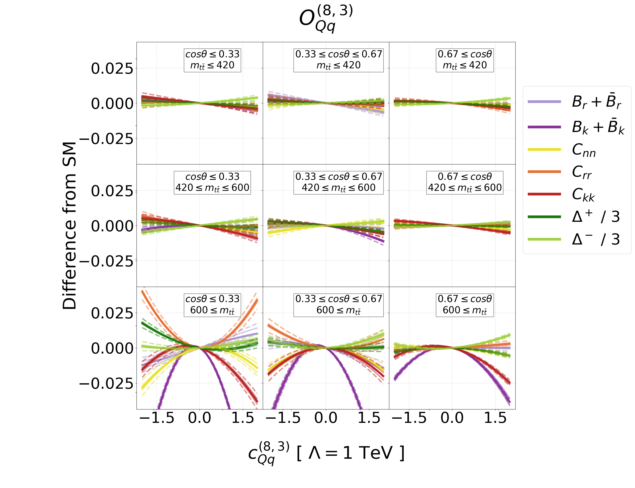
Refer to caption
Refer to caption
Figure 8: Results for the operators 𝒪Qq(8,3)superscriptsubscript𝒪𝑄𝑞83\mathcal{O}_{Qq}^{(8,3)} (top) and 𝒪Qq(1,3)superscriptsubscript𝒪𝑄𝑞13\mathcal{O}_{Qq}^{(1,3)} (bottom), similar to Figure 5.
Refer to caption
Refer to caption
Figure 9: Results for the operators 𝒪Qu8superscriptsubscript𝒪𝑄𝑢8\mathcal{O}_{Qu}^{8} (top) and 𝒪Qu1superscriptsubscript𝒪𝑄𝑢1\mathcal{O}_{Qu}^{1} (bottom), similar to Figure 5.
Refer to caption
Refer to caption
Figure 10: Results for the operators 𝒪tq8superscriptsubscript𝒪𝑡𝑞8\mathcal{O}_{tq}^{8} (top) and 𝒪tq1superscriptsubscript𝒪𝑡𝑞1\mathcal{O}_{tq}^{1} (bottom), similar to Figure 5.
Refer to caption
Refer to caption
Figure 11: Results for the operators 𝒪Qd8superscriptsubscript𝒪𝑄𝑑8\mathcal{O}_{Qd}^{8} (top) and 𝒪Qd1superscriptsubscript𝒪𝑄𝑑1\mathcal{O}_{Qd}^{1} (bottom), similar to Figure 5.
Refer to caption
Refer to caption
Figure 12: Results for the operators 𝒪tu8superscriptsubscript𝒪𝑡𝑢8\mathcal{O}_{tu}^{8} (top) and 𝒪tu1superscriptsubscript𝒪𝑡𝑢1\mathcal{O}_{tu}^{1} (bottom), similar to Figure 5.
Refer to caption
Refer to caption
Figure 13: Results for the operators 𝒪td8superscriptsubscript𝒪𝑡𝑑8\mathcal{O}_{td}^{8} (top) and 𝒪td1superscriptsubscript𝒪𝑡𝑑1\mathcal{O}_{td}^{1} (bottom), similar to Figure 5.

References

  • (1) A. Buckley, C. Englert, J. Ferrando, D.J. Miller, L. Moore, M. Russell et al., Constraining top quark effective theory in the LHC Run II era, JHEP 04 (2016) 015 [1512.03360].
  • (2) D. Barducci et al., Interpreting top-quark LHC measurements in the standard-model effective field theory, 1802.07237.
  • (3) N.P. Hartland, F. Maltoni, E.R. Nocera, J. Rojo, E. Slade, E. Vryonidou et al., A Monte Carlo global analysis of the Standard Model Effective Field Theory: the top quark sector, JHEP 04 (2019) 100 [1901.05965].
  • (4) I. Brivio, S. Bruggisser, F. Maltoni, R. Moutafis, T. Plehn, E. Vryonidou et al., O new physics, where art thou? A global search in the top sector, JHEP 02 (2020) 131 [1910.03606].
  • (5) J. Ellis, M. Madigan, K. Mimasu, V. Sanz and T. You, Top, Higgs, Diboson and Electroweak Fit to the Standard Model Effective Field Theory, JHEP 04 (2021) 279 [2012.02779].
  • (6) SMEFiT collaboration, Combined SMEFT interpretation of Higgs, diboson, and top quark data from the LHC, JHEP 11 (2021) 089 [2105.00006].
  • (7) ATLAS collaboration, Observation of spin correlation in tt¯𝑡¯𝑡t\bar{t} events from pp collisions at sqrt(s) = 7 TeV using the ATLAS detector, Phys. Rev. Lett. 108 (2012) 212001 [1203.4081].
  • (8) ATLAS collaboration, Measurements of spin correlation in top-antitop quark events from proton-proton collisions at s=7𝑠7\sqrt{s}=7 TeV using the ATLAS detector, Phys. Rev. D 90 (2014) 112016 [1407.4314].
  • (9) CMS collaboration, Measurement of Spin Correlations in tt¯𝑡¯𝑡t\bar{t} Production using the Matrix Element Method in the Muon+Jets Final State in pp𝑝𝑝pp Collisions at s=𝑠absent\sqrt{s}= 8 TeV, Phys. Lett. B 758 (2016) 321 [1511.06170].
  • (10) CMS collaboration, Measurements of t t-bar spin correlations and top quark polarization using dilepton final states in pp collisions at sqrt(s) = 8 TeV, Phys. Rev. D 93 (2016) 052007 [1601.01107].
  • (11) ATLAS collaboration, Measurements of top quark spin observables in tt¯𝑡¯𝑡t\overline{t} events using dilepton final states in s=8𝑠8\sqrt{s}=8 TeV pp collisions with the ATLAS detector, JHEP 03 (2017) 113 [1612.07004].
  • (12) CMS collaboration, Measurement of the top quark polarization and tt¯t¯t\mathrm{t\bar{t}} spin correlations using dilepton final states in proton-proton collisions at s=𝑠absent\sqrt{s}= 13 TeV, Phys. Rev. D 100 (2019) 072002 [1907.03729].
  • (13) ATLAS collaboration, Measurement of the tt¯𝑡¯𝑡t\bar{t} production cross-section and lepton differential distributions in eμ𝑒𝜇e\mu dilepton events from pp𝑝𝑝pp collisions at s=13TeV𝑠13TeV\sqrt{s}=13\,\text{TeV} with the ATLAS detector, Eur. Phys. J. C 80 (2020) 528 [1910.08819].
  • (14) ATLAS collaboration, Measurements of top-quark pair spin correlations in the eμ𝑒𝜇e\mu channel at s=13𝑠13\sqrt{s}=13 TeV using pp𝑝𝑝pp collisions in the ATLAS detector, Eur. Phys. J. C 80 (2020) 754 [1903.07570].
  • (15) Y. Afik and J.R.M.n. de Nova, Entanglement and quantum tomography with top quarks at the LHC, Eur. Phys. J. Plus 136 (2021) 907 [2003.02280].
  • (16) Y. Afik and J.R.M.n. de Nova, Quantum information with top quarks in QCD production, 2203.05582.
  • (17) J.A. Aguilar-Saavedra and J.A. Casas, Improved tests of entanglement and Bell inequalities with LHC tops, Eur. Phys. J. C 82 (2022) 666 [2205.00542].
  • (18) R. Aoude, E. Madge, F. Maltoni and L. Mantani, Quantum SMEFT tomography: Top quark pair production at the LHC, Phys. Rev. D 106 (2022) 055007 [2203.05619].
  • (19) M. Fabbrichesi, R. Floreanini and G. Panizzo, Testing Bell Inequalities at the LHC with Top-Quark Pairs, Phys. Rev. Lett. 127 (2021) 161801 [2102.11883].
  • (20) C. Severi, C.D.E. Boschi, F. Maltoni and M. Sioli, Quantum tops at the LHC: from entanglement to Bell inequalities, Eur. Phys. J. C 82 (2022) 285 [2110.10112].
  • (21) A.J. Barr, Testing Bell inequalities in Higgs boson decays, Phys. Lett. B 825 (2022) 136866 [2106.01377].
  • (22) A.J. Barr, P. Caban and J. Rembieliński, Bell-type inequalities for systems of relativistic vector bosons, 2204.11063.
  • (23) J.A. Aguilar-Saavedra, A. Bernal, J.A. Casas and J.M. Moreno, Testing entanglement and Bell inequalities in HZZ𝐻𝑍𝑍H\to ZZ, 2209.13441.
  • (24) J.A. Aguilar-Saavedra, Laboratory-frame tests of quantum entanglement in HWW𝐻𝑊𝑊H\to WW, 2209.14033.
  • (25) R. Ashby-Pickering, A.J. Barr and A. Wierzchucka, Quantum state tomography, entanglement detection and Bell violation prospects in weak decays of massive particles, 2209.13990.
  • (26) M. Fabbrichesi, R. Floreanini and E. Gabrielli, Constraining new physics in entangled two-qubit systems: top-quark, tau-lepton and photon pairs, 2208.11723.
  • (27) W. Bernreuther, D. Heisler and Z.-G. Si, A set of top quark spin correlation and polarization observables for the LHC: Standard Model predictions and new physics contributions, JHEP 12 (2015) 026 [1508.05271].
  • (28) M. Czakon, A. Mitov and R. Poncelet, NNLO QCD corrections to leptonic observables in top-quark pair production and decay, JHEP 05 (2021) 212 [2008.11133].
  • (29) C. Degrande, G. Durieux, F. Maltoni, K. Mimasu, E. Vryonidou and C. Zhang, Automated one-loop computations in the standard model effective field theory, Phys. Rev. D 103 (2021) 096024 [2008.11743].
  • (30) B. Grzadkowski, M. Iskrzynski, M. Misiak and J. Rosiek, Dimension-Six Terms in the Standard Model Lagrangian, JHEP 10 (2010) 085 [1008.4884].
  • (31) C. Zhang and S. Willenbrock, Effective-Field-Theory Approach to Top-Quark Production and Decay, Phys. Rev. D 83 (2011) 034006 [1008.3869].
  • (32) B. Grzadkowski and Z. Hioki, Decoupling of anomalous top decay vertices in angular distribution of secondary particles, Phys. Lett. B 557 (2003) 55 [hep-ph/0208079].
  • (33) J.A. Aguilar-Saavedra, J. Carvalho, N.F. Castro, F. Veloso and A. Onofre, Probing anomalous Wtb couplings in top pair decays, Eur. Phys. J. C 50 (2007) 519 [hep-ph/0605190].
  • (34) A. Czarnecki, M. Jezabek and J.H. Kuhn, Lepton Spectra From Decays of Polarized Top Quarks, Nucl. Phys. B 351 (1991) 70.
  • (35) A. Brandenburg, Z.G. Si and P. Uwer, QCD corrected spin analyzing power of jets in decays of polarized top quarks, Phys. Lett. B 539 (2002) 235 [hep-ph/0205023].
  • (36) J.M. Campbell and R.K. Ellis, Top-Quark Processes at NLO in Production and Decay, J. Phys. G 42 (2015) 015005 [1204.1513].
  • (37) J.M. Campbell, R.K. Ellis, P. Nason and E. Re, Top-Pair Production and Decay at NLO Matched with Parton Showers, JHEP 04 (2015) 114 [1412.1828].
  • (38) A. Denner, S. Dittmaier, S. Kallweit and S. Pozzorini, NLO QCD corrections to WWbb production at hadron colliders, Phys. Rev. Lett. 106 (2011) 052001 [1012.3975].
  • (39) G. Bevilacqua, M. Czakon, A. van Hameren, C.G. Papadopoulos and M. Worek, Complete off-shell effects in top quark pair hadroproduction with leptonic decay at next-to-leading order, JHEP 02 (2011) 083 [1012.4230].
  • (40) P. Artoisenet, R. Frederix, O. Mattelaer and R. Rietkerk, Automatic spin-entangled decays of heavy resonances in Monte Carlo simulations, JHEP 03 (2013) 015 [1212.3460].
  • (41) R. Frederix, I. Tsinikos and T. Vitos, Probing the spin correlations of tt¯𝑡¯𝑡t{\bar{t}} production at NLO QCD+EW, Eur. Phys. J. C 81 (2021) 817 [2105.11478].
  • (42) W. Bernreuther, M. Fuecker and Z.-G. Si, Weak interaction corrections to hadronic top quark pair production, Phys. Rev. D 74 (2006) 113005 [hep-ph/0610334].
  • (43) NNPDF collaboration, Parton distributions from high-precision collider data, Eur. Phys. J. C 77 (2017) 663 [1706.00428].
  • (44) CMS collaboration, Projection of the top quark spin correlation measurement and search for top squark pair production at the HL-LHC, .
  • (45) V. Shtabovenko, R. Mertig and F. Orellana, FeynCalc 9.3: New features and improvements, Comput. Phys. Commun. 256 (2020) 107478 [2001.04407].