[en-US]ord=raise

Graph gauge theory of mobile non-Abelian anyons in a qubit stabilizer code

Abstract

Stabilizer codes allow for non-local encoding and processing of quantum information. Deformations of stabilizer surface codes introduce new and non-trivial geometry, in particular leading to emergence of long sought after objects known as projective Ising non-Abelian anyons. Braiding of such anyons is a key ingredient of topological quantum computation. We suggest a simple and systematic approach to construct effective unitary protocols for braiding, manipulation and readout of non-Abelian anyons and preparation of their entangled states. We generalize the surface code to a more generic graph with vertices of degree 2, 3 and 4. Our approach is based on the mapping of the stabilizer code defined on such a graph onto a model of Majorana fermions charged with respect to two emergent gauge fields. One gauge field is akin to the physical magnetic field. The other one is responsible for emergence of the non-Abelian anyonic statistics and has a purely geometric origin. This field arises from assigning certain rules of orientation on the graph known as the Kasteleyn orientation in the statistical theory of dimer coverings. Each 3-degree vertex on the graph carries the flux of this “Kasteleyn” field and hosts a non-Abelian anyon. In our approach all the experimentally relevant operators are unambiguously fixed by locality, unitarity and gauge invariance. We illustrate the power of our method by making specific prescriptions for experiments verifying the non-Abelian statistics.

Topological quantum computation^{1, 2, 3} can be realized by a macroscopic quantum system with a few controllable collective degrees of freedom, called non-Abelian anyons. Multiple non-Abelian anyons define a Hilbert space, whose dimension is set by the number and type of non-Abelian anyons. States in this Hilbert space encode information non-locally. Hence they can serve as a quantum memory protected from local perturbations. Quantum gates that process this quantum information are to be implemented through exchanges of pairs of anyons that braid their space-time trajectories [see Fig. 1(a)]. A double braiding of identical non-Abelian anyons, an exchange of the positions of a pair of anyons twice that returns them to a locally indistinguishable state, may nonetheless change physical observables of the system. Since the braiding outcome of non-Abelian anyons are insensitive to details of the anyon trajectories the implementation of quantum gates by braiding non-Abelian anyons are topologically protected.

A simple construction of non-Abelian anyons is based on Majorana fermions $\alpha_{j}$, satisfying $\{\alpha_{j},\alpha_{k}\}=2\delta_{jk}$. Two Majorana operators define a parity for a complex fermion with number $n$, $i\alpha_{2}\alpha_{1}=(-1)^{n}$. Separating them in space is sufficient to realize quantum memory. We now describe how Ising non-Abelian^{4, 5, 6} braiding arises for Majorana fermions bound to $\pi$ flux, following an argument of Ivanov ⁷ for the case of $p+ip$ superconductors. Consider a system of four Majoranas, $\alpha_{i},i=1,..,4$, in Fig. 1(b-c). Bringing Majoranas together allows local measurement of the fermion parity $i\alpha_{2}\alpha_{1}$. Double braiding of $\alpha_{3}$ and $\alpha_{2}$ [see Fig. 1(c)] is equivalent to moving $\alpha_{2}$ around $\alpha_{3}$ [see Fig. 1(b)]. Since Majorana $\alpha_{3}$ carries $\pi$ flux and the Majorana $\alpha_{2}$ carries charge, the latter picks up a phase $\alpha_{2}\rightarrow-\alpha_{2}$ similarly to Aharonov-Bohm effect. Therefore the fermion parity $i\alpha_{2}\alpha_{1}$ changes sign. Hence this double braiding results in a rotation in the Hilbert space of anyons. In other words, if $i\alpha_{2}\alpha_{1}$ is identified with a Pauli $Z$ operator, the braiding realizes an $X$ logical gate. However, despite decades of research^{8, 7, 4, 9, 10, 11, 12, 13, 14} non-Abelian anyons were never unambiguously observed in experiment.

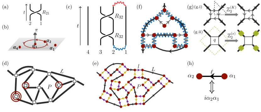
Figure 1: (a) A schematic of the counter-clockwise swap $R_{12}$ of two anyons 1 and 2. (b) Aharonov-Bohm effect of flux-bound Majorana fermions. (c) Double braid of anyons 2 and 3. The wavy blue/red line show fermion parity operator defined before/after the double braiding operation. (d) Plaquette surface code graph with qubits drawn as gray diamonds. D3Vs are marked with red circles and a D2V is marked with a double-circle. (e) The decorated version of the PSC graph in Fig. 1 (d) with Kasteleyn orientation. Red dots correspond to Majorana fermions. Black links connect different qubits, and yellow and purple links are intra qubit. (f) An example counter-clockwise canonical loop enclosing a single $\sigma$. (g) The two emergent $\mathbb{Z}_{2}$ gauge symmetries in our model. Both local symmetry actions correspond to (contractible) loops in the dual graph shown in dashed lines. (g.i) the $\mathbb{Z}_{2}^{(K)}$ symmetry transformation from one Kasteleyn orientation to another flips all arrows touching a vertex. (g.ii) the $\mathbb{Z}_{2}^{(s)}$ symmetry transformation generated by $\Gamma_{q}$ flips all $L$-type links touching the diamond $q$. (h) A diagrammatic rule for assigning directed edges to Majorana bilinears on the $\ell$-edges.

Recent development of gate based quantum processors¹⁵ provides a new avenue for direct preparation of a many-body quantum state without involving the Hamiltonian and the difficulty in reaching its ground state. We introduce the plaquette surface code (PSC) as a stabilizer code¹⁶ defined on a specific type of qubit graph [see Fig. 1(d)]. As in any stabilizer code, the multi-qubit state $\ket{\psi}$ can be prepared to satisfy commuting constraints,

$$B(P)\ket{\psi}=\ket{\psi},$$ (1)

where $B(P)$ are operators called stabilizers for each plaquette $P$ of the qubit graph [see Fig. 1(d)]. The states $\ket{\psi}$ satisfying Eq. (1) form the code subspace. A state $\ket{\phi}$ with $B(P^{\prime})\ket{\phi}=-\ket{\phi}$ for a plaquette $P^{\prime}$ has a “stabilizer flux” at $P^{\prime}$. In the rest of the paper, we focus on states with few to no stabilizer fluxes. In the PSC, the qubits form vertices of a surface graph, which only contains degree 4 (D4Vs), degree 3 (D3Vs), and degree 2 (D2Vs) vertices [See Fig. 1(d)]. We will show D3V’s host Ising anyons.

The standard surface codes (on manifolds with and without boundary) ^{1, 17, 18, 19} are a special case of the PSC. Kitaev ⁶ pointed out the topological degrees of freedom at dislocations of the square lattice, and Bombin ²⁰ and Kitaev and Kong ²¹ pointed out that such dislocations act as non-Abelian Ising anyons when they are introduced to the toric code ground state¹. This observation motivated efforts to exploit the projective non-Abelian nature ^{22, 23, 24} of the so-called “twist defects” which were found to carry Majoranas ^{25, 26}. However, the microscopic mechanism of flux attachment was not identified and a protocol for moving the defects unitarily is absent. Moreover, manipulation of anyons can be realized by code deformation, i.e. reconfiguration of the stabilizers and the movement of the edges of the graph. In absence of the microscopic gauge theory, the design of optimal anyon manipulation protocols is challenging. The operational use of the graph in our approach is to define directed paths. Those directed paths enable us to simply and systematically find all essential operators: the stabilizers, unitary operators for dynamics, and Hermitian operators for the logical qubit state measurements.

In this paper, we explicitly identify a gauge field responsible for the flux attachment on a graph, and demonstrate its purely geometric origin. By formulating a new graph gauge theory, we construct optimal unitary protocols for projective Ising anyon state preparation and braiding, and predict specific experimental outcomes. Note that the surface codes were recently implemented on gate based NISQ superconducting processors^{15, 27}. Our unitary protocols are advantageous for such platforms since for them unitary operations are typically faster than measurement based protocols by an order of magnitude.

As usual the gauge field is associated with a global conserved quantity. On any graph $G$ where all vertices are of degree 2, 3, and 4, the number $N_{\sigma}=N_{\text{D3V}}+2N_{\text{D2V}}=0\mod 2$, where $N_{\text{D}j\text{V}}$ is the number of degree $j$ vertices, is conserved $(\mathrm{mod}\;2)$. In fact, the value of $N_{\sigma}$ also has an important physical consequence and associated conservation law: if there are $N_{S}$ stabilizer plaquettes, Euler’s formula for the Euler characteristic $\chi(M)$ yields

$$N_{Q}-N_{S}=\frac{N_{\sigma}}{2}-\chi(M),$$ (2)

where we take our surface graph on some manifold with boundary $M$. From this formula we find that the dimension of the code subspace in the most important case, $M$ topologically a disk, is $\max\{2^{N_{\sigma}/2-1},1\}$. This is the first hint that each $\sigma$ corresponds to non-local degrees of freedom, as each is roughly “half” a qubit. Importantly, if the number of stabilizers is fixed, $N_{\sigma}$ is conserved.

To make the conservation of $N_{\sigma}$ more manifest, we decorate each qubit vertex with a diamond as shown in Fig. 1(e). On the decorated graph $\tilde{G}$, $N_{\sigma}$ is the number of vertices with two incident edges, which we call $\sigma$ or “unpaired”. We construct a field which assigns flux to these vertices in a particular way.

First, we need a local rule to lift directed paths $\gamma$ through the “physical” qubit graph $G$ [Fig. 1(d)] to directed paths $\tilde{\gamma}$ through $\tilde{G}$ [Fig. 1(e)]: every diamond is traversed counter-clockwise [Fig. 1(f)]. Such paths $\tilde{\gamma}$ are called canonical. Our field is the assignment of arrows to each link, which follows the local rule that an odd number are clockwise about each face (such an orientation is called Kasteleyn³¹). We find [See Fig. 1(f) and Appendix B]

$$(-1)^{N_{\sigma}(\tilde{\gamma})}=-\prod_{\ell\in\text{Edges}(\tilde{\gamma})}(-1)^{n^{(K)}_{\ell}(\tilde{\gamma})},$$ (3)

for any counter-clockwise canonical loop $\tilde{\gamma}$, where $n^{(K)}_{\ell}(\tilde{\gamma})$ is 1 (0) if the arrow on the edge $\ell$ is in the opposite (same) direction as $\tilde{\gamma}$, and $N_{\sigma}(\tilde{\gamma})$ is the number of $\sigma$ enclosed by the loop $\tilde{\gamma}$. The Kasteleyn orientation is not unique: for example, flipping all the arrows touching a vertex is a local $\mathbb{Z}_{2}$ transformation (which we call $\mathbb{Z}_{2}^{(K)}$) from one Kasteleyn orientation to another [See Fig. 1(g.i)], while manifestly preserving Eq. 3 [See also Appendix B]. In this sense, we have attached flux of a $\mathbb{Z}_{2}$ field to the $\sigma$.

We now place a Majorana at each vertex of the decorated graph, Fig. 1(e). An orientation is natural in a theory of Majorana fermions on a graph: after assigning a direction, links $\ell$ with an arrow $\alpha_{j}\to\alpha_{k}$ define a Hermitian fermion parity [See Fig. 1 (h)]

$$(-1)^{n_{\ell}}=i\alpha_{k}\alpha_{j}.$$ (4)

The link operator is clearly not invariant under choice of particular Kasteleyn structure. Since the $\mathbb{Z}_{2}^{(K)}$ transformation at a vertex hosting Majorana $\alpha_{j}$ flips all the link operators involving $\alpha_{j}$, we can think of the Majoranas as “charged” under the local $\mathbb{Z}_{2}^{(K)}$ symmetry. If physical meaning could be given to canonical paths, the Majoranas at $\sigma$ vertices would be bound to $\pi$ flux. We describe a qubit model, the PSC, where there is both an emergent Kasteleyn structure as well as a second $\mathbb{Z}_{2}$ field associated to a gauge transformation we call $\mathbb{Z}_{2}^{(s)}$ [See Fig. 1(g.ii)]. Keeping the second field flat ensures Wilson lines in the gauge theory maintain a canonical form under local unitary evolution. Moreover, since no physical observable depends on the particular Kasteleyn orientation chosen, in other words $\mathbb{Z}_{2}^{(K)}$ is gauged, the Majoranas at $\sigma$ vertices are bound to $\pi$ flux of a gauge field.

We start by using the Kasteleyn orientation on the decorated graph to explicitly determine two standard elements defining a gauge theory: the physical subspace of the Majorana Hilbert space (giving rise to $\mathbb{Z}_{2}^{(s)}$), and the mapping from physical qubits into the subspace. Recall we placed a Majorana at each vertex of the decorated graph, so that each qubit $q$ of the PSC corresponds to a diamond with 4 Majoranas. Note that at each diamond, opposite links $l_{a},l_{b}$ do not touch, so the operators [See Fig. 2(a)] $\tau_{1}=(-1)^{n_{l_{a}}},\tau_{1}^{\prime}=(-1)^{n_{l_{b}}}$ satisfy $\tau_{1}^{2}=\tau_{1}^{\prime 2}=1,[\tau_{1},\tau_{1}^{\prime}]=0$, and neither can be proportional to $1$ since they anti-commute with the other pair of link operators. In a qubit Hilbert space, these conditions imply that $\tau_{1}=\pm\tau_{1}^{\prime}$, and the choice $\tau_{1}=\tau_{1}^{\prime}$ in the qubit space gives rise to the physical subspace condition [see Fig. 2(b)]

$$\Gamma_{q}\ket{\psi}=\ket{\psi},\;\Gamma_{q}=(-1)^{n_{l_{a}}}(-1)^{n_{l_{b}}}.$$ (5)

The Kasteleyn condition ensures that as an operator $\Gamma_{q}$ is independent of the chosen pair of edges, so if we construct $\tau_{2},\tau_{2}^{\prime}$ in an analogous way for the other pair we also find $\tau_{2}=\tau_{2}^{\prime}$ in the physical subspace. $\Gamma_{q}$ generates a local gauge transformation $\mathbb{Z}_{2}^{(s)}$ under which each Majorana fermion carries a charge, i.e. $\alpha_{qj}$ changes sign upon conjugation with $\Gamma_{q}$. The second ingredient of the gauge structure, a mapping from qubits to the Majoranas, is fixed by choosing a qubit operator to correspond to each pair of opposing edges, e.g. Pauli operators $\tau_{1}=Z$ and $\tau_{2}=X$. Note that, by construction, the spin operators defined by the $l$-type links, $\tau_{1},\tau_{2}$, are invariant under $\mathbb{Z}_{2}^{(s)}$ and $\mathbb{Z}_{2}^{(K)}$.

Stabilizers and $\mathbb{Z}_{2}^{(s)}$ – The final ingredient to define our gauge theory is a local flatness condition for the $\mathbb{Z}_{2}^{(s)}$ gauge field formed by the inter-diamond $L$-type link operators. In contrast to the intra-diamond $l$-type link operators, which are $\mathbb{Z}_{2}^{(s)}$-invariant, $L$-type link operators all commute (since these links never touch) but are odd under both $\mathbb{Z}^{(s)}_{2}$ and $\mathbb{Z}_{2}^{(K)}$ [See Fig. 1(g)]. Specifically, the $\mathbb{Z}_{2}^{(s)}$ transformation flips all $(-1)^{n_{L}}$ touching a diamond. The simplest $\mathbb{Z}_{2}^{(s)}$-invariant combination is a loop of $L$-type edges around a stabilizer plaquette $P$,

$$B(P)=\prod_{L\in P}(-1)^{n_{L}}.$$ (6)

Moreover, by writing $B(P)$ in terms of the gauge-invariant $l$-type link operators (this is a special case of Eq. 11), we find that it is $\mathbb{Z}_{2}^{(K)}$ invariant as well. This gives both the definition of and physical meaning to the stabilizers defining the PSC code subspace alluded to in Eq. 1.

Emergence of $\mathbb{Z}_{2}^{(K)}$ – Since the Kasteleyn orientation is not a conventional $\mathbb{Z}_{2}$ gauge field, let us briefly describe an alternative construction of the same theory where the gauge structure is emergent. A consistent mapping from the single qubit Hilbert space into a fixed parity sector of 4 Majoranas is fully specified ³³by associating a diamond with Kasteleyn orientation to the qubit, and pairs of opposite edges on the diamond to two generators of the Pauli algebra, as above. Extending this construction to a multi-qubit system, by additionally assigning arrows to $L$-type links the corresponding (gauge-non-invariant and hence unphysical) operators combine to measure a (physical) $\mathbb{Z}_{2}^{(s)}$ gauge flux Eq. 6. If the arrows are assigned so that every plaquette has a Kasteleyn orientation, $B(P)$ is simply a product of Pauli operators at each diamond determined by the local embedding at each qubit of the plaquette, regardless of the size or shape of $P$. We note that a static graph with a preferred mapping between qubits and Majoranas dictated by a Hamiltonian, as in the model studied by Kitaev ⁶, may fix part of the Kasteleyn structure. However, as D3Vs and D2Vs move, the PSC evolves. In this case, the emergent $\mathbb{Z}_{2}^{(K)}$ plays a critical role in tracking the PSC evolution.

Having defined the complete gauge theory, we consider two families of multi-qubit operators that act on the PSC state, distinguished by the condition that they generate stabilizer flux only at controlled locations³⁶. Acting with a Majorana on a given vertex flips the edge operators $(-1)^{n_{\ell}}$ for every edge $\ell$ touching the vertex, creating a pair of stabilizer fluxes if the vertex is not unpaired [See Fig. 2(c.i)]. The local condition not to create stabilizer flux is to flip an even number of $L$-type edge operators around each plaquette: either acting with Majoranas on both ends of an $L$-type edge, i.e., $(-1)^{n_{L}}$ [See Fig. 2(c.ii)], or to flip 2 or more $L$-type links about each stabilizer plaquette [See Fig. 2(c.iii)]. Combined with local gauge invariance, the first method builds Wilson lines³⁸, while the second builds ’t Hooft lines³⁹.

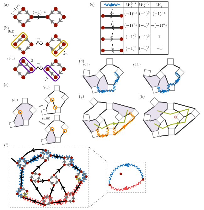
Figure 2: (a) The parity operators on the $l$-edges and $L$-links. (b) Pauli operator $\tau_{1},\tau_{2}$ assignment to the diamond edges $\{\tau_{1},\tau_{2}\}=0$. For instance, $\tau_{1}=Z$ and $\tau_{2}=X$. (c) Two examples of how to locally avoid creating stabilizer flux, ignoring gauge invariance. (c.i) Acting with the Majorana circled in orange flips the $L$-link it touches, and creates $\varepsilon$, i.e., a pair of stabilizer fluxes sharing an edge, shown in lavender. (c.ii) The basis for the Wilson line. Flip the same $L$-link again by acting with a second Majorana touching the link. (c.iii) The basis for the ’t Hooft line. Flip an even number of $L$-links. (d) Augmented Wilson lines: (d.i) An example of a canonical augmented Wilson line action on a state with no stabilizer flux. The link at the start of the line is flipped, creating an $\varepsilon$, while there is no bond to flip at the unpaired vertex. If there were an $\varepsilon$ particle at the start of the line, this augmented Wilson line would “sink” it into the unpaired vertex, removing any stabilizer flux. (d.ii) A non-canonical Wilson line. (e) The diagrammatic rules for constructing a Wilson line operator from a directed path on the graph. The blue wavy arrow indicates the orientation of the path $\gamma$. The black and gray arrows indicate Kasteleyn orientation on the $L$-links and on the $l$-edges respectively. (f) Two canonical augmented Wilson lines between the same pair of unpaired vertices. We show the common part of the two lines, which in this case lie on the first and last links, in dark yellow. (g) An open ’t Hooft line is shown in moss green, with stabilizer fluxes at its ends. The shown ’t Hooft line is equivalent to the gauge-invariant Wilson line segments shown in orange. (h) An open ’t Hooft line wrapping an unpaired vertex, marked with a red circle, creating an $\varepsilon$ from a state with no stabilizer flux.

Wilson lines – Flipping each $L$-type link twice means we act with $L$-link operators, which manifestly commute with $B(P)$. While $(-1)^{n_{L}}$ is not gauge invariant under $\mathbb{Z}_{2}^{(s)}$, if we chain $L$-link operators (connected by diamonds), the bulk of the chain commutes with $\Gamma_{q}$. To make the ends of the chain $\mathbb{Z}_{2}^{(s)}$ invariant, we must add an additional Majorana from the diamonds at the ends, arriving at the definition of a valid path for the augmented Wilson line in Fig. 2(d). Formally, a valid path is one that starts and ends on $l$-links. To give a definition of an operator that is both consistent with the Majorana anti-commutation relations and invariant under $\mathbb{Z}_{2}^{(K)}$, we take the path $\gamma$ (from $\alpha_{I}\to\alpha_{F}$) to be directed. Explicitly, the gauge-invariant “augmented Wilson line” associated to the path $\gamma$ is defined by [See Fig. 2(e)]

$$\mathcal{W}_{\gamma} =i\alpha_{F}W_{\gamma}\alpha_{I},\;W_{\gamma}=W^{(s)}_{\gamma}W^{(K)}_{\gamma}$$ (7)

$$W^{(s)}_{\gamma} =\prod_{L\in\gamma}(-1)^{n_{L}},\;W^{(K)}_{\gamma}=\prod_{\ell\in\gamma}(-1)^{n^{(K)}_{\ell}(\gamma)},$$ (8)

where we refer to $W_{\gamma}$ as the Wilson line. If the line is open, its ends are either paired or unpaired vertices. If the vertex is paired, a pair of stabilizer fluxes sharing an edge are created when acting on a state with no stabilizer flux: we call such flux configurations an $\varepsilon$-particle¹ [See Fig. 2(d)]. No stabilizer flux is created at an unpaired end.

Wilson loops and line deformations – When $\gamma$ is a (directed) loop the Wilson loop $W_{\gamma}$, which can be defined by the same Eqs. 7 and 8, is gauge invariant on its own. We define the augmented Wilson loop (Eq. 7 is not defined for coinciding ends) as $\mathcal{W}_{\gamma}=-W_{\gamma}$ (to emphasize the type we sometimes write $\mathcal{W}^{(\text{loop})}_{\gamma}$). A canonical counter-clockwise augmented Wilson loop measures the parity of stabilizer and Kasteleyn flux:

$$\mathcal{W}^{(\text{loop})}_{\gamma}=(-1)^{N_{\Phi}(\gamma)}(-1)^{N_{\sigma}(\gamma)},$$ (9)

where $N_{\Phi}(\gamma)$ is the operator measuring the stabilizer flux enclosed by the loop. It is practically useful that the operator $B(P)$ is just the counter-clockwise augmented Wilson loop about only the stabilizer plaquette $P$: one perspective is that $B(P)$ should only count the stabilizer flux $B(P)=(-1)^{N_{\Phi}(P)}$, so is not equivalent to a canonical loop in the presence of anyons. The most important application is to the ratio of canonical Wilson lines for two paths $\gamma,\gamma^{\prime}$ between same anyons 1 and 2 [See Fig. 2(f)]. The gauge-invariant operator $\mathcal{W}_{\gamma}\mathcal{W}_{\gamma^{\prime}}^{-1}=W_{\gamma}W_{\gamma^{\prime}}^{-1}$ can be decomposed to a product of canonical augmented Wilson loops, such that for canonical paths

$$\mathcal{W}_{\gamma}\mathcal{W}_{\gamma^{\prime}}^{-1}=W_{\gamma}W_{\gamma^{\prime}}^{-1}=(-1)^{N_{\Phi}(\gamma,\gamma^{\prime})}(-1)^{N_{\sigma}(\gamma,\gamma^{\prime})}.$$ (10)

where $N_{\Phi}(\gamma,\gamma^{\prime})$ is the stabilizer flux enclosed between the paths, whereas $N_{\sigma}(\gamma,\gamma^{\prime})$ is the number of enclosed anyons (see Appendix B.1 for the precise definition, which is only needed when one of the paths $\gamma,\gamma^{\prime}$ goes directly through a diamond containing an anyon away from the endpoints of $\gamma,\gamma^{\prime}$, and therefore does not play an important role in braiding).

’t Hooft lines and loops – We represent an ’t Hooft line³⁹ as a directed path of even length through the dual graph, whose links represent the flipped $L$-type bonds [See Fig. 2(g)]. The definition ensures that we can always find a local, gauge-invariant operator corresponding to the ’t Hooft line. Specifically, an ’t Hooft line can be written as a product of augmented Wilson lines by taking the Majoranas to the right of the path which touch the links crossed, and making this product gauge invariant in the most local way [See Fig. 2(g)]. If the path is open, stabilizer fluxes are created at its ends. Flips corresponding to odd length paths through the dual lattice are always products of ’t Hooft lines and an augmented Wilson line with one unpaired end. Finally, we note that ’t Hooft loops create no flux; for simplicity, we always take such loops counter-clockwise.

’t Hooft and canonical Wilson lines – Two relationships between the two families of operators are of particular importance. First, note that a Wilson and ’t Hooft line anti-commute at each point of crossing, because ’t Hooft lines flip $L$-type links. Since $\varepsilon$ live at the end of augmented Wilson lines [See Fig. 2(d)], roughly speaking ’t Hooft loops detect the parity of enclosed $\varepsilon$. More importantly, certain ’t Hooft lines going around a single anyon counter-clockwise are equivalent, in a no-flux state, to canonical Wilson lines [See Fig. 3(a)]. Specifically, an ’t Hooft line going around a single anyon counter-clockwise cannot be closed to a non-intersecting loop. The ends can be brought to adjacent plaquettes, where an $\varepsilon$ will be created [See Fig. 2(h)]. This acts in the same way as an augmented Wilson line starting at the anyon and ending at the $\varepsilon$. As we demonstrate in Fig. 3(a), the augmented Wilson line that has the same action including the global phase can always be taken to follow a canonical path.

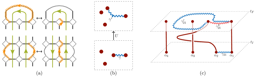
Figure 3: (a) Examples of an explicit deformation of ’t Hooft lines (moss green) to augmented Wilson line (orange) (left) and canonical Wilson lines (right), in a state with no stabilizer flux. (b) Motion of the anyon $2$ generated by a local unitary $U$, acting only on a region containing anyon $2$. (c) A manifestly gauge invariant illustration of Ising anyon braiding in the long-distance limit, tracking the extending augmented Wilson line and the world line of the anyons. The augmented Wilson lines associated with $\gamma_{21}$ and $\gamma_{21}^{\prime\prime}$ are measured before and after the double braid respectively. The comparison between the two measurements should only depend on the topological form of the motion of $\alpha_{2}$.

Extension of canonical lines – General principles of gauge theory³⁸ dictate that the Wilson line $W_{\gamma}$ between $\alpha_{1}$ and $\alpha_{2}$, associated to the augmented Wilson line $\mathcal{W}_{\gamma}$, should “extend” when $\alpha_{2}$ moves by a local unitary $U$ starting from a state $\ket{\psi}$. Specifically, locality, unitarity, and gauge invariance determine the key aspects of the path $\gamma^{\prime}$ one should take after moving $\alpha_{2}$ so that $W_{\gamma^{\prime}}$ “acts the same way” as $W_{\gamma}$. Explicitly, as shown in Fig. 3(b) the path $\gamma^{\prime}$ is just an extension of $\gamma$ into the region where $U$ acts and ending at the new location of $\alpha_{2}$, so that $\mathcal{W}_{\gamma^{\prime}}U\ket{\psi}=U\mathcal{W}_{\gamma}\ket{\psi}$. This way, the Wilson line keeps track of the path and history of the anyons.

Therefore, the last key ingredient of our theory of non-Abelian anyons is the requirement that Wilson lines are extended by motion. This is the physical condition which distinguishes canonical Wilson lines: any local unitary $U$ acting in a region $A$ with a single anyon, without stabilizer flux and preserving the anyon and stabilizer flux number, extends any canonical Wilson line between anyons to a canonical Wilson line. In most cases, this can be seen by taking a canonical Wilson line ending at the anyon and extending beyond $A$, and (partially) expanding it to an ’t Hooft line that lies strictly outside $A$; the first steps of this expansion are shown on the right column of Fig. 3(a). Acting with the unitary cannot change the action of the ’t Hooft line on the state. Therefore, we can deform the ’t Hooft line to a necessarily canonical Wilson line ending at the new position of the anyon. Without this fundamental property, the behaviour of Wilson lines would depend on non-topological details of the dynamics. Instead, referring to Eq. 10, we find that unpaired Majoranas carry both a $\pi$ flux and charge of the Kasteleyn field.

As discussed in the introduction, we can now conclude that the unpaired Majoranas, or D3Vs, in our model are projective Ising anyons. To illustrate this point directly, we formulate a simple braid to unambiguously demonstrate non-Abelian statistics (see Fig. 1(c)). Initialize the system at time $t_{I}$ with four anyons arranged on a line, and suppose measurement of $\mathcal{W}_{\gamma_{21}}$ yields the value $+1$ [See Fig. 3(c)]. As we move $\alpha_{2}$ around $\alpha_{3}$, the path $\gamma_{21}$ gets extended to a path $\gamma_{21}^{\prime}$ around $\alpha_{3}$. The measurement of $\mathcal{W}_{\gamma_{21}^{\prime\prime}}$ at time $t_{F}$ will give $-1$, since it is different from the measurement of $\mathcal{W}_{\gamma_{21}}$ at time $t_{I}$ by $W_{\gamma_{21}^{\prime}}W_{\gamma_{21}^{\prime\prime}}^{-1}=-1$ by Eq. 10 ($N_{\Phi}(\gamma_{21}^{\prime},\gamma_{21}^{\prime\prime})=0,N_{\sigma}(\gamma_{21}^{\prime},\gamma_{21}^{\prime\prime})=1$). In other words an observable changes sign after double braiding with probability 1, which is sufficient to demonstrate non-Abelian statistics. On the other hand, if $\alpha_{3}$ was attached to a stabilizer flux the observable will not change sign since now $N_{\Phi}(\gamma_{21}^{\prime},\gamma_{21}^{\prime\prime})=1$, so braiding about such a composite could serve as a control experiment. We note that the composites are on equal footing to what we consider the “bare” anyons, and our notion of which anyon is a composite would switch if we had chosen to prefer the opposite chirality, clockwise instead of counter-clockwise, in the definition of the Kasteleyn structure and preferred loops. In particular, amongst themselves the composites braid precisely as projective Ising anyons as well.

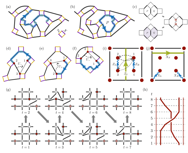
Figure 4: (a) A valid path defining an augmented Wilson line. The static assignement of the Pauli operators are indicated by yellow for $Z$ and purple for $X$. In this case, $N_{ll}(\gamma)=3$ in Eq. 11. (b) A Wilson loop enclosing a stabilizer plaquette $P$. The Wilson loop operator graphically specifies the stabilizer $B(P)$. (c) Deleting an $L$-link in the graph creates two unpaired vertices marked with red circles. It also changes the stabilizers. If we take the new definition, $B(P^{\prime})\ket{\psi}=\ket{\psi}$ whether or not there was a fermion on $P,Q$, without any unitary operation. This is a microscopic manifestation of the fusion rule $\sigma\times\sigma=1+\varepsilon$. (d) A basic edge move generated by a counter-clockwise augmented Wilson line shown in blue. Since the path is counter-clockwise, $U_{-}$ should be used to avoid creating $\mathbb{Z}_{2}^{(s)}$ flux. The vertex $3$, initially paired with $2$, pairs with $1$ after the edge move leaving $2$ unpaired. (e) A basic edge move generated by a clockwise augmented Wilson line shown in blue. $U_{+}$ should be used to avoid creating $\mathbb{Z}_{2}^{(s)}$ flux. (f) Clockwise Wilson line with an anyon along the path. Since $N_{ll}(\gamma)=1$, one needs to use $U_{-}$ to avoid creating $\mathbb{Z}_{2}^{(s)}$ flux. (g) A protocol for implementing the braid group generator Fig. 1(a) and restoring the lattice. We show a 10-qubit section for concreteness, but on a larger device the anyons could be further separated. (h) The time slices corresponding to the protocol in Fig. 4(g). (i) The protocol for preparing a GHZ state of three logical qubits. Four anyons at the corner and the two pairs created in the bulk together supply three logical qubits. The vertical ’t Hooft line (moss green) and the two augmented Wilson lines (wavy blue) measures the logical qubit state. Dashed braiding or dotted braiding will both entangle the logical qubits to yield a GHZ state. (j) The protocol for implementing the logical X operator.

Below we suggest specific protocols and predict outcomes for several experiments.

Spin operators for augmented Wilson lines and loops – We will use augmented Wilson lines and loops as the basis for all physical operations, so it will only be necessary to give a qubit-space formula for these operators. Fortunately, they can be constructed simply and systematically from paths drawn on the decorated PSC graph (without assigning any explicit Kasteleyn orientation). First, assign diamonds to each qubit, and two Pauli generators, say $X$ and $Z$, to pairs of opposite edges on each diamond [Fig. 4(a)]. In general, we call the Pauli associated to the $l$-link $\tau_{l}$, and we keep this assignment static. Now, $L$-type edges are drawn between diamond vertices to construct a PSC graph. Given a valid directed path $\gamma$ in this graph, we simply read off the operator along the path

$$\mathcal{W}_{\gamma}=(-i)^{N_{ll}(\gamma)}\overleftarrow{\prod_{l\in\gamma}}\tau_{l}.$$ (11)

For multi-qubit loops $\gamma$, we delete an $L$-link and apply Eq. 11 to the resulting open path. Here $N_{ll}(\gamma)$ is the number of vertices in $\gamma$ with adjacent $l$-edges [See Fig. 4(a)]. The arrow over the product specifies that the product is to be taken in order from right to left according to the path: $\tau_{l}$ for the earliest $l$ appears at right end. ’t Hooft lines are constructed using the correspondence to products of augmented Wilson lines in Fig. 2 (g). We note that to make the rules of the protocol simple, we will use both canonical and non-canonical lines and loops.

Stabilizers and initial state – As an immediate application, we recall that the stabilizers $B(P)$ are simply the unique counter-clockwise Wilson loops, generally not canonical, in the stabilizer plaquette $P$ [See Fig. 4b]. Hence, Eq. (11) offers the necessary input for a protocol to prepare a state in the code space of the PSC ¹⁵.

Creation, measurement, and fusion – The creation of anyon pairs only requires the removal of an $L$-type link [See Fig. 4(c) top]. When we modify the graph by deleting an edge, we do not need to perform unitary action for the operators obtained on the new graph to remain meaningful in the new code subspace. The link touches at least one stabilizer plaquette $P$. If the link is a boundary link, we simply drop $B(P)$ from the list of stabilizers. If the link touches another plaquette, $Q$, deleting the edge forms a larger plaquette $P^{\prime}$, and we find $B(P^{\prime})=B(P)B(Q)$. Notice that if we remove a link shared by the stabilizer fluxes of an $\varepsilon$, we also end up in the no stabilizer flux state of two additional anyons [See Fig. 4(c) bottom]. This embodies the Ising anyon fusion rule⁶

$$\sigma\times\sigma=1+\varepsilon.$$ (12)

Since arbitrary unitary motion preserves canonical Wilson lines, if we wish to determine the fusion state of separated anyons we should measure a canonical Wilson line between them (according to the path along which they would be physically fused). We could also measure the equivalent ’t Hooft loop around the anyon pair, but this is generally less efficient. We note that the other $\sigma$ fusion rule $\sigma\times\varepsilon=\sigma$ is simply a consequence of the fact that Wilson lines can terminate on an anyon without creating flux, while $\varepsilon\times\varepsilon=1$ is an immediate consequence of the definition of $\varepsilon$.

Gauge-invariant Majorana swaps – Since $L$-type links pair Majoranas, edge rearrangements in the graph correspond to Majorana swaps. Naively, to “move” Majoranas from position 1 to position 2, i.e., $\alpha_{1}\to\pm\alpha_{2}$ with some unitary $\tilde{U}_{\pm}$, we mean $\tilde{U}_{\pm}^{\dagger}\alpha_{2}\tilde{U}_{\pm}=\pm\alpha_{1}$. If $\alpha_{1},\alpha_{2}$ are on different Majorana diamonds $q,q^{\prime}$, such a $\tilde{U}_{\pm}$ cannot be gauge invariant. The reason is that $\{\Gamma_{q},\alpha_{1}\}=0$, but $[\Gamma_{q},\alpha_{2}]=0$, so necessarily $[\Gamma_{q},\tilde{U}_{\pm}]\neq 0$. In other words, $\tilde{U}_{\pm}$ takes the state away from the gauge-invariant Hilbert space. The simplest non-gauge invariant swap is $\tilde{U}_{\pm}=\exp\left(\pm\frac{\pi}{4}\alpha_{2}\alpha_{1}\right)$, which also takes $\alpha_{2}\to\mp\alpha_{1}$. The closest gauge invariant operator requires a path $\gamma$ from $\alpha_{1}\to\alpha_{2}$, from which we define,

$$U_{\pm}=\exp\left(\mp i\frac{\pi}{4}\mathcal{W}_{\gamma}\right).$$ (13)

For this particular unitary, we can see explicitly how Wilson lines are extended as the Majoranas are swapped

$$U_{\pm}^{\dagger}(\gamma)\alpha_{2}W_{\gamma}U_{\pm}(\gamma)=\pm\alpha_{1},\;U_{\pm}^{\dagger}(\gamma)\alpha_{1}U_{\pm}(\gamma)=\mp\alpha_{2}W_{\gamma}.$$ (14)

We note that as long as a PSC is chosen where all the $\tau_{l}$ are Pauli operators, $U_{\pm}$ is always in the Clifford group, and can therefore be decomposed efficiently to $\operatorname{CNOT}$ (or $\operatorname{CZ}$) and single-qubit Clifford gates.

Gates for moving anyons – Graphically, moving a single anyon from vertex 1 to vertex 2 corresponds to a rearrangment of $L$-type links [See Figs. 4(d-f)]. The corresponding swaps Eq. 13 are built from paths $\gamma$ that run between an anyon $\alpha_{1}$ and a Majorana $\alpha_{2}$ paired by an $L$-type edge to $\alpha_{3}$ [See Figs. 4 (d-f)]. To ensure the graph remains locally planar, it is sufficient to build larger moves from elements where $\alpha_{1}$ and $\alpha_{2}$ share the same stabilizer plaquette $P$. There is a unique allowed path $\gamma$ between them within $P$. Similarly to the line for $B(P)$, in general this path is not canonical. The sign in Eq. 13 is determined by the condition that no flux is created in the new graph (with an $L$-type edge between 1 and 3). Specifically, if the path $\gamma$ is counter-clockwise about the plaquette containing $\alpha_{2}$ and $\alpha_{1}$, we use the $U_{-}$ [See Fig. 4(d)]. If the path is clockwise about this plaquette, we find $U_{\zeta}$ with $\zeta=(-1)^{N_{ll}(\gamma)}$ where $N_{ll}(\gamma)$ is the number of vertices with adjacent $l$-type edges in $\gamma$, defined in Eq. 11 [see Figs. 4(e) and (f)]. By construction, this is an example of a unitary motion of anyons without creation of $\mathbb{Z}_{2}^{(s)}$ flux. It follows that the canonicity of Wilson lines connecting anyons is always preserved, despite the fact we chose to use a non-canonical line give the rules for the unitaries. Finally, we remark that to move the composite of an anyon and $\mathbb{Z}_{2}^{(s)}$ flux, one simply uses the opposite sign in $U_{\pm}$ to the one for the bare anyon.

Braid generators – Figures 4(g-h) show one minimal implementation of the fundamental generator of the braid group, $R_{23}$. All other generators can be constructed in an analogous manner. One advantage of this protocol is that it restores the lattice: practically, this means such generators can be iterated an arbitrary number of times, and theoretically it allows directly comparing states before and after braiding. Another advantage is that it can be implemented on small systems, and simply extended to make use of larger ones. The version shown requires only 10 qubits and can therefore be implemented on existing devices ¹⁵. A direct experiment to establish non-Abelian statistics is to perform the lattice version of Fig. 3 (c): simply create two anyons from the vacuum at the locations $t=1$, and perform this braid twice to implement $R_{23}^{2}$. After $R_{23}^{2}$ each pair of anyons will fuse to an $\varepsilon$.

In the future, periodic measurements of stabilizers would allow quantum error correction, with the distance between anyons serving as an effective code distance. On a larger device, extending the protocol in Figs. 4(g-h) simply by starting the anyons further apart, and continuing the vertical motion of the initially rightmost anyon at $t=3$, would allow maintaining a larger code distance. The protocol involves local code deformations, as a result of which the graph and stabilizer sizes change, but the most non-local stabilizers can be restricted to be the smallest possible 5-local operators. We leave the analysis of this overhead to future work.

A GHZ experiment – Another key element of topological quantum computation is preparation of an entangled state of anyons. We give a protocol such that a single braid takes a logical product state $\ket{000}$ to a GHZ state⁴³, which is a starting point for the discussion of multi-qubit entanglement. Our protocol also serves as a concise demonstration of computational primitives introduced above. Observe that the standard surface code encoding one logical qubit is nothing else than our model with 4 Ising anyons at the corners ⁴⁴. We define logical $Z$ operators using the shortest Wilson lines for bulk anyons and an ’t Hooft line for the anyons at the corners, [See Fig. 4(i)]. The ’t Hooft line is chosen to run down the center of the sample, so that anyon pairs can be on either side. When it splits anyon pairs, such an ’t Hooft line is shorter than any equivalent Wilson line.

To prepare the logical state $\ket{000}$, it is simplest to start from the $\ket{0}$ state of the surface code, and create anyon pairs from the vacuum at the locations shown in Fig. 4(i). An exchange of bulk anyons 1 and 2 then prepares a state of the form $\ket{\text{GHZ}_{\phi}}=\frac{1}{\sqrt{2}}(\ket{000}+e^{i\phi}\ket{111})$, where $\phi$ depends on the phase choice of the logical basis. To fix an unambiguous convention for $\phi$ and perform full tomography, it is sufficient to define logical $X$ operators as in Fig. 4(j). Then exchange of anyons 1 and 2 prepares $\ket{\text{GHZ}_{\pi/2}}$. An exchange of anyons 1 and 3, which can be generated by conjugating the above braid with an exchange of 2 and 3, prepares $\ket{\text{GHZ}_{0}}$.

To summarize, we constructed a graph gauge theory with projective Ising anyons. The consistency of the theory requires identification of two gauge fields: one associated with the flux created by a plaquette (stabilizer) violation and the other, the Kasteleyn orientation, is associated with the flux carried by a D3V, degree three vertex of the graph. The presence of both fields ensures that a loop physical path of an unpaired Majorana fermion measures the number of unpaired Majoranas enclosed by it, giving rise to non-Abelian braiding statistics. The formulation of physical operators in terms of augmented Wilson lines and the graphical rules to construct them allows a simple way to design unitary protocols for manipulation and measurement of anyons. The unitary evolution can be thought of as the motion of anyons directly realizing elementary braiding operations. We propose specific experiments to realize the dynamics of anyons and verify their fusion rules and braiding statistics as well as preparation of an entangled state of anyons. The protocols we proposed were implemented experimentally on a superconducting processor as reported in the forthcoming publication. Our recipe for constructing protocols could be used to realize quantum computation with non-Abelian anyons that allows for quantum error correction. 

Acknowlegements: YL gratefully acknowledges conversations with Felipe Hernandez and Chao-Ming Jian. We also thank Eduardo Fradkin, Bert Halperin, Trond Andersen, Pedram Roushan and members of Quantum AI for discussions. YL and EAK acknowledges support by a New Frontier Grant from Cornell University’s College of Arts and Sciences. EAK acknowledges support by the NSF under OAC-2118310, the Ewha Frontier 10-10 Research Grant, and the Simons Fellowship in Theoretical Physics award 920665. EAK performed a part of this work at the Aspen Center for Physics, which is supported by the National Science Foundation grant PHY-160761.

Appendix A Appendix

Appendix B A. Examples on a $5\times 5$ qubit system

In this section, we illustrate some of the above steps explicitly in a $5\times 5$ qubit system. First, we specify the initial state by giving appropriate stabilizers, see Fig. 5(a). The initial PSC is simply a square graph in the bulk, with 4 anyons at the corners: this is just a surface code encoding 1 qubit ¹⁸, and has previously been prepared on a superconducting quantum processor¹⁵. We assume the state can be prepared so that the vertical ’t Hooft line shown, whose explicit form is also given, takes a definite value.

Next, in Fig 5(b) we show the Pauli string that generates a motion that appears in the middle of a possible extension of the braid in Fig. 4(g) to a larger system. According to the rules from the main text, we use Eq. 13 with $U_{+}$ to perform this move. As discussed in the main text, if we wished to move the composite of an anyon with attached $\mathbb{Z}_{2}^{(s)}$ flux, we would use $U_{-}$.

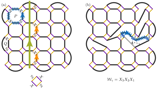
Figure 5: (a) The surface code as a PSC, with several visualizations of Eq. 11. We show the two stabilizers associated to the plaquettes $P$ and $Q$, as well as the Wilson line for $B(P)$. We also apply the rules from Fig. 2(g) to construct the Pauli string for the logical $Z$ ’t Hooft line (the Pauli string appears to the right of the line). (b) The Pauli string that generates a movement circuit, associated to the Wilson line shown. This is another direct application of Eq. 11.

Appendix C B. Kasteleyn orientations and path deformations

A Kasteleyn orientation ³¹ always exists on a surface graph with an even number of vertices ^{46, 47}. There is a precise sense in which such an orientation behaves like a typical $\mathbb{Z}_{2}$ gauge field. One Kasteleyn orientation can be taken to any other by flipping arrows on links crossed by cycles through the dual graph ^{46, 47}, with contractible cycles generated by the $\mathbb{Z}_{2}^{(K)}$ transformation described in the main text. This is the same way that a conventional $\mathbb{Z}_{2}$ field configuration can be taken to any other with the same pattern of local flux (the transformations corresponding to the contractible loops are gauge). The reason is that any cycle flips an even number of arrows in each plaquette.

We will re-use the definition $W^{(K)}_{\gamma}$ from Eq. 8 for directed paths and loops in a general graph (i.e. it is $+1$ ($-1$) if there are an even (odd) number of arrows along the path that point opposite the direction of the path). Importantly, the above discussion proves that for a directed contractible loop $\gamma$, $W^{(K)}_{\gamma}$ is independent of the choice of Kasteleyn orientation. The invariant value can be understood by contracting a simple (no self-intersections) counter-clockwise loop to a single face $F_{0}$, where the definition of a Kasteleyn orientation is that $W^{(K)}_{\partial F_{0}}=-1$. To do this, we give a useful rule for “pushing” segments of a path $\gamma$ through a face $F$. Part of $\partial F$ is $\gamma_{1}\subset\gamma$. The complement of $\gamma_{1}$ in the boundary $\partial F$ of the face $F$ is $\gamma_{2}$. To “deform” the path $\gamma$ is to replace $\gamma_{1}$ with $\gamma_{2}$ (in the same direction), obtaining a path $\gamma^{\prime}$. To compute the accompanying sign change $W^{(K)}_{\gamma}(W^{(K)}_{\gamma^{\prime}})^{-1}$, note that $\gamma_{2}$ traverses $F$ clockwise, so the Kasteleyn condition for $F$ refers to the reversed path $\hat{R}\gamma_{2}$. We have the general formula $W_{\hat{R}\gamma}^{(K)}=(-1)^{\operatorname{length}(\gamma)}W_{\gamma}^{(K)}=-(-1)^{\operatorname{vertices}(\gamma)}W_{\gamma}^{(K)}$. Combining with the Kasteleyn condition, we find in the case of deformation through a single face

$$W^{(K)}_{\gamma_{1}}=(-1)^{\operatorname{vertices}(\gamma_{2})-2}W_{\gamma_{2}}^{(K)}.$$ (15)

But $\operatorname{vertices}(\gamma_{2})-2$ simply counts the number of vertices that are in the interior of $\gamma$ but not $\gamma^{\prime}$. Continuing this way until we arrive at a single face, calling $V_{B}(\gamma)$ the number of vertices in the interior of the loop $\gamma$ we find

$$W^{(K)}_{\gamma}=-(-1)^{V_{B}(\gamma)}$$

for any counter-clockwise simple loop $\gamma$.

C.1 B.1 Canonical paths and loops

We now return to the special case of the decorated PSC graph, and always focus on a disk-like region. Every simple counter-clockwise loop in the undecorated graph, $\hat{\gamma}$, could naturally correspond to $2^{\operatorname{length}(\hat{\gamma})}$ directed loops through the decorated graph, because at each added diamond we can choose whether to go around it clockwise or counter-clockwise.

For open paths we also choose which diamond vertex the path ends at. The physical requirement of $\mathbb{Z}^{(s)}_{2}$ invariance for the augmented Wilson lines that are built from this path constrains it to end on a different vertex of the endpoint diamonds than where it entered. This is the definition of a valid path.

In fact, we can see by inspection of Eqs. 7 and 8 that the choice of how diamonds are traversed only affects the Kasteleyn part of a loop or line, and therefore simply changes the sign of the operator. Moreover, by the deformation formula Eq. 15 we see that if a line touches a diamond an odd number of times, it does not matter which way we traverse that diamond. Thus we only have to keep careful track of “wedges” where a diamond is touched precisely twice in a row. When building various operators this can simply be chosen as convenient (c.f. the movement gates in Fig. 4(d-f)), but to predict braiding outcomes by deformation of Wilson lines we need to know which way to take the wedges. Remarkably, unitarity, locality, and gauge invariance determine that we can always take Wilson lines with wedges pointing to the right (i.e. traversing the diamond counter-clockwise) to measure fusion outcomes. In the main text, to give a more concise definition of canonicity we simply insisted on all lines traversing the diamonds counter-clockwise, which is equivalent to the definition here. The more refined definition here is convenient for various proofs since fewer cases need to be checked. Note in particular $(-1)^{N_{ll}(\gamma)}$ (defined below Eq. 11) only depends on the number of wedges.

Consider now a simple canonical loop $\gamma$, and cut away the exterior edges and vertices, so that $\gamma$ becomes the boundary of a graph $\tilde{G}$. The important geometric property of a canonical loop is that, when viewed as the boundary of $\tilde{G}$, $\gamma$ has an even number of odd degree vertices. By the “handshaking lemma” ⁴⁸, this means that the number of odd-degree vertices on the interior of the loop is even. The only even-degree vertices are the unpaired ones, so $V_{B}(\gamma)=N_{\sigma}(\gamma)$ and for a contractible canonical loop

$$W^{(K)}_{\gamma}=-(-1)^{N_{\sigma}(\gamma)}.$$

This proves the results Eqs. 3 and 9.

To prove Eq. 10, we note that, as usual, the ratio of the Kasteleyn Wilson lines, $W^{(K)}_{\gamma}(W^{(K)}_{\gamma^{\prime}})^{-1}$ of two valid canonical paths $\gamma,\gamma^{\prime}$ with endpoints at the same two anyons 1,2 is a product of ratios of canonical paths that form simple closed loops. Each loop consists of two segments, one from $\gamma$ and one from $\gamma^{\prime}$. We only need to consider one such loop. One of the segments is counter-clockwise about the loop and the other clockwise; call the counter-clockwise segment $\gamma_{1}$ and the other $\gamma_{2}$. In fact, by enumerating the ways in which canonical paths can split from each other, one finds that $\gamma_{2}$ is always valid (this is not necessarily the case for $\gamma_{1}$). The reversed path $\hat{R}\gamma_{2}$ may not be canonical, and $W_{\hat{R}(\gamma_{2})}^{(K)}=-(-1)^{N_{ll}(\gamma_{2})}W_{\gamma_{2}}^{(K)}$. To make the reversed path canonical, each wedge should be flipped, which cancels the factor $(-1)^{N_{ll}(\gamma_{2})}$; call this path $R\gamma_{2}$. The path $\gamma=\gamma_{1}\cup R\gamma_{2}$ is now a canonical loop, and we find

$$W_{\gamma_{1}}^{(K)}(W_{\gamma_{2}}^{(K)})^{-1}=-W_{\gamma}^{(K)}=(-1)^{N_{\sigma}(\gamma)}\equiv(-1)^{N_{\sigma}(\gamma_{1},\gamma_{2})}.$$

This expression gives a precise definition of $N_{\sigma}(\gamma,\gamma^{\prime})$ in the main text, which is only necessary when the Wilson lines pass directly through unpaired anyons away from the endpoints (the latter are of course in common, and it is straightforward to check that they never contribute to this flux difference). In practice, if there are few anyons on the Wilson line it is often simpler to deform the line by one plaquette using Eq. 15 first, and then apply the counting formula. We also note that because of some exceptions at the endpoints, in the main text we only stated Eq. 10 for Wilson lines between anyons. The formula also applies with other conditions, most obviously when the paths $\gamma,\gamma^{\prime}$ differ only away from their endpoint diamonds.

References

- Kitaev [2003] A. Y. Kitaev, Fault-tolerant quantum computation by anyons, Annals of Physics 303, 2 (2003), arXiv:quant-ph/9707021 .
- Nayak et al. [2008] C. Nayak, S. H. Simon, A. Stern, M. Freedman, and S. D. Sarma, Non-Abelian Anyons and Topological Quantum Computation, Reviews of Modern Physics 80, 1083 (2008), arXiv:0707.1889 .
- Stern [2010] A. Stern, Non-Abelian states of matter, Nature 464, 187 (2010).
- Moore and Read [1991] G. Moore and N. Read, Nonabelions in the fractional quantum hall effect, Nuclear Physics B 360, 362 (1991).
- Nayak and Wilczek [1996] C. Nayak and F. Wilczek, 2n-quasihole states realize 2n-1-dimensional spinor braiding statistics in paired quantum Hall states, Nuclear Physics B 479, 529 (1996).
- Kitaev [2006] A. Kitaev, Anyons in an exactly solved model and beyond, Annals of Physics 321, 2 (2006), arXiv:cond-mat/0506438 .
- Ivanov [2001] D. A. Ivanov, Non-abelian statistics of half-quantum vortices in p-wave superconductors, Physical Review Letters 86, 268 (2001), arXiv:cond-mat/0005069 .
- Read and Green [2000] N. Read and D. Green, Paired states of fermions in two dimensions with breaking of parity and time-reversal symmetries, and the fractional quantum Hall effect, Physical Review B 61, 10267 (2000), arXiv:cond-mat/9906453 .
- Bonderson et al. [2006] P. Bonderson, A. Kitaev, and K. Shtengel, Detecting Non-Abelian Statistics in the nu=5/2 Fractional Quantum Hall State, Physical Review Letters 96, 016803 (2006).
- Clarke et al. [2011] D. J. Clarke, J. D. Sau, and S. Tewari, Majorana fermion exchange in quasi-one-dimensional networks, Physical Review B 84, 035120 (2011), arXiv:1012.0296 [cond-mat] .
- Alicea et al. [2011] J. Alicea, Y. Oreg, G. Refael, F. von Oppen, and M. P. A. Fisher, Non-Abelian statistics and topological quantum information processing in 1D wire networks, Nature Physics 7, 412 (2011), arXiv:1006.4395 [cond-mat] .
- Lindner et al. [2012] N. H. Lindner, E. Berg, G. Refael, and A. Stern, Fractionalizing Majorana fermions: Non-abelian statistics on the edges of abelian quantum Hall states, Physical Review X 2, 041002 (2012), arXiv:1204.5733 [cond-mat] .
- Stern and Lindner [2013] A. Stern and N. H. Lindner, Topological Quantum Computation—From Basic Concepts to First Experiments, Science 339, 1179 (2013).
- Clarke et al. [2013] D. J. Clarke, J. Alicea, and K. Shtengel, Exotic non-Abelian anyons from conventional fractional quantum Hall states, Nature Communications 4, 1348 (2013), arXiv:1204.5479 [cond-mat] .
- Satzinger et al. [2021] K. J. Satzinger, Y. Liu, A. Smith, C. Knapp, M. Newman, C. Jones, Z. Chen, C. Quintana, X. Mi, A. Dunsworth, C. Gidney, I. Aleiner, F. Arute, K. Arya, J. Atalaya, R. Babbush, J. C. Bardin, R. Barends, J. Basso, A. Bengtsson, A. Bilmes, M. Broughton, B. B. Buckley, D. A. Buell, B. Burkett, N. Bushnell, B. Chiaro, R. Collins, W. Courtney, S. Demura, A. R. Derk, D. Eppens, C. Erickson, E. Farhi, L. Foaro, A. G. Fowler, B. Foxen, M. Giustina, A. Greene, J. A. Gross, M. P. Harrigan, S. D. Harrington, J. Hilton, S. Hong, T. Huang, W. J. Huggins, L. B. Ioffe, S. V. Isakov, E. Jeffrey, Z. Jiang, D. Kafri, K. Kechedzhi, T. Khattar, S. Kim, P. V. Klimov, A. N. Korotkov, F. Kostritsa, D. Landhuis, P. Laptev, A. Locharla, E. Lucero, O. Martin, J. R. McClean, M. McEwen, K. C. Miao, M. Mohseni, S. Montazeri, W. Mruczkiewicz, J. Mutus, O. Naaman, M. Neeley, C. Neill, M. Y. Niu, T. E. O’Brien, A. Opremcak, B. Pató, A. Petukhov, N. C. Rubin, D. Sank, V. Shvarts, D. Strain, M. Szalay, B. Villalonga, T. C. White, Z. Yao, P. Yeh, J. Yoo, A. Zalcman, H. Neven, S. Boixo, A. Megrant, Y. Chen, J. Kelly, V. Smelyanskiy, A. Kitaev, M. Knap, F. Pollmann, and P. Roushan, Realizing topologically ordered states on a quantum processor, Science 374, 1237 (2021), arXiv:2104.01180 .
- Gottesman [1997] D. Gottesman, Stabilizer Codes and Quantum Error Correction, arXiv:quant-ph/9705052 (1997), arXiv:quant-ph/9705052 .
- Wen [2003] X.-G. Wen, Quantum orders in an exact soluble model, Physical Review Letters 90, 016803 (2003), arXiv:quant-ph/0205004 .
- Bravyi and Kitaev [1998] S. B. Bravyi and A. Y. Kitaev, Quantum codes on a lattice with boundary, arXiv:quant-ph/9811052 (1998), arXiv:quant-ph/9811052 .
- Freedman and Meyer [1998] M. H. Freedman and D. A. Meyer, Projective plane and planar quantum codes (1998), arXiv:quant-ph/9810055 .
- Bombin [2010] H. Bombin, Topological Order with a Twist: Ising Anyons from an Abelian Model, Physical Review Letters 105, 030403 (2010), arXiv:1004.1838 [cond-mat, physics:hep-th, physics:quant-ph] .
- Kitaev and Kong [2012] A. Kitaev and L. Kong, Models for gapped boundaries and domain walls, Communications in Mathematical Physics 313, 351 (2012), arXiv:1104.5047 [cond-mat] .
- Barkeshli et al. [2013] M. Barkeshli, C.-M. Jian, and X.-L. Qi, Theory of defects in Abelian topological states, Physical Review B 88, 235103 (2013).
- You and Wen [2012] Y.-Z. You and X.-G. Wen, Projective non-Abelian Statistics of Dislocation Defects in a Z_N Rotor Model, Physical Review B 86, 161107 (2012), arXiv:1204.0113 [cond-mat, physics:quant-ph] .
- Benhemou et al. [2021] A. Benhemou, J. K. Pachos, and D. E. Browne, Non-Abelian statistics with mixed-boundary punctures on the toric code, arXiv:2103.08381 [quant-ph] (2021), arXiv:2103.08381 [quant-ph] .
- Zheng et al. [2015] H. Zheng, A. Dua, and L. Jiang, Demonstrating non-Abelian statistics of Majorana fermions using twist defects, Physical Review B 92, 245139 (2015), arXiv:1508.04166 .
- Brown et al. [2017] B. J. Brown, K. Laubscher, M. S. Kesselring, and J. R. Wootton, Poking holes and cutting corners to achieve Clifford gates with the surface code, Physical Review X 7, 021029 (2017), arXiv:1609.04673 [cond-mat, physics:quant-ph] .
- Acharya et al. [2022] R. Acharya, I. Aleiner, R. Allen, T. I. Andersen, M. Ansmann, F. Arute, K. Arya, A. Asfaw, J. Atalaya, R. Babbush, D. Bacon, J. C. Bardin, J. Basso, A. Bengtsson, S. Boixo, G. Bortoli, A. Bourassa, J. Bovaird, L. Brill, M. Broughton, B. B. Buckley, D. A. Buell, T. Burger, B. Burkett, N. Bushnell, Y. Chen, Z. Chen, B. Chiaro, J. Cogan, R. Collins, P. Conner, W. Courtney, A. L. Crook, B. Curtin, D. M. Debroy, A. D. T. Barba, S. Demura, A. Dunsworth, D. Eppens, C. Erickson, L. Faoro, E. Farhi, R. Fatemi, L. F. Burgos, E. Forati, A. G. Fowler, B. Foxen, W. Giang, C. Gidney, D. Gilboa, M. Giustina, A. G. Dau, J. A. Gross, S. Habegger, M. C. Hamilton, M. P. Harrigan, S. D. Harrington, O. Higgott, J. Hilton, M. Hoffmann, S. Hong, T. Huang, A. Huff, W. J. Huggins, L. B. Ioffe, S. V. Isakov, J. Iveland, E. Jeffrey, Z. Jiang, C. Jones, P. Juhas, D. Kafri, K. Kechedzhi, J. Kelly, T. Khattar, M. Khezri, M. Kieferová, S. Kim, A. Kitaev, P. V. Klimov, A. R. Klots, A. N. Korotkov, F. Kostritsa, J. M. Kreikebaum, D. Landhuis, P. Laptev, K.-M. Lau, L. Laws, J. Lee, K. Lee, B. J. Lester, A. Lill, W. Liu, A. Locharla, E. Lucero, F. D. Malone, J. Marshall, O. Martin, J. R. McClean, T. Mccourt, M. McEwen, A. Megrant, B. M. Costa, X. Mi, K. C. Miao, M. Mohseni, S. Montazeri, A. Morvan, E. Mount, W. Mruczkiewicz, O. Naaman, M. Neeley, C. Neill, A. Nersisyan, H. Neven, M. Newman, J. H. Ng, A. Nguyen, M. Nguyen, M. Y. Niu, T. E. O’Brien, A. Opremcak, J. Platt, A. Petukhov, R. Potter, L. P. Pryadko, C. Quintana, P. Roushan, N. C. Rubin, N. Saei, D. Sank, K. Sankaragomathi, K. J. Satzinger, H. F. Schurkus, C. Schuster, M. J. Shearn, A. Shorter, V. Shvarts, J. Skruzny, V. Smelyanskiy, W. C. Smith, G. Sterling, D. Strain, M. Szalay, A. Torres, G. Vidal, B. Villalonga, C. V. Heidweiller, T. White, C. Xing, Z. J. Yao, P. Yeh, J. Yoo, G. Young, A. Zalcman, Y. Zhang, and N. Zhu, Suppressing quantum errors by scaling a surface code logical qubit (2022), arXiv:2207.06431 [quant-ph] .
- Note [1] As a consequence of the “handshaking lemma” that every graph has an even number of odd degree vertices48.
- Note [2] On a general manifold there may be relations amongst the stabilizers that depend on topology and boundary conditions which can increase the effective code subspace.
- Note [3] In other words, an anyon with the quantum dimension .
- Kasteleyn [1963] P. W. Kasteleyn, Dimer Statistics and Phase Transitions, Journal of Mathematical Physics 4, 287 (1963).
- Note [4] Kasteleyn structures were introduced to study dimer models31, and were later related to 2D spin structures46, 47.
- Note [5] More precisely, up to a global phase, which for us is irrelevant.
- Note [6] Note that we have given the analogous condition, an odd number of clockwise arrows in each plaquette, for the Kasteleyn orientation.
- Note [7] In general, the same would be true if we fixed the parity of clockwise edges across all stabilizer plaquettes.
- Fradkin [2013] E. Fradkin, Field Theories of Condensed Matter Physics, 2nd ed. (Cambridge University Press, Cambridge, 2013).
- Note [8] More precisely, we will find violations of different type are created in pairs at the ends of string operators.
- Wilson [1974] K. G. Wilson, Confinement of quarks, Physical Review D 10, 2445 (1974).
- ’t Hooft [1978] G. ’t Hooft, On the phase transition towards permanent quark confinement, Nuclear Physics B 138, 1 (1978).
- Note [9] Equivalently, since ’t Hooft loops measure parity and deform to canonical augmented Wilson lines.
- Note [10] More complicated braids can achieve larger code distances by constant factors in certain cases.
- Note [11] The precise procedure to accomplish this depends slightly on the available geometry when the devices are small, for example in many cases it is convenient to modify the step from to by moving edges to the right instead of the left of the anyon to move it upwards. Such an extension is shown in Appendix A.
- Greenberger et al. [2007] D. M. Greenberger, M. A. Horne, and A. Zeilinger, Going Beyond Bell’s Theorem (2007), arXiv:0712.0921 [quant-ph] .
- Bravyi et al. [2018] S. Bravyi, M. Englbrecht, R. Koenig, and N. Peard, Correcting coherent errors with surface codes, npj Quantum Information 4, 55 (2018), arXiv:1710.02270 [quant-ph] .
- Note [12] In our system of Ising anyons Clifford gates can be implemented fault-tolerantly. A non-Clifford -gate necessary for universal computation can be constructed by replacing in Eq. (13) and taking the line between any two anyons. This operation is not fault-tolerant.
- Cimasoni and Reshetikhin [2007] D. Cimasoni and N. Reshetikhin, Dimers on surface graphs and spin structures. I, Communications in Mathematical Physics 275, 187 (2007), arXiv:math-ph/0608070 .
- Cimasoni and Reshetikhin [2008] D. Cimasoni and N. Reshetikhin, Dimers on surface graphs and spin structures. II, Communications in Mathematical Physics 281, 445 (2008), arXiv:0704.0273 [math-ph] .
- Euler [1741] L. Euler, Solutio problematis ad geometriam situs pertinentis, Commentarii academiae scientiarum Petropolitanae , 128 (1741).