Lattice QCD study of antiheavy-antiheavy-light-light tetraquarks based on correlation functions with scattering interpolating operators both at the source and at the sink

Abstract

We present first results of a recently started lattice QCD investigation of antiheavy-antiheavy-light-light tetraquark systems including scattering interpolating operators in correlation functions both at the source and at the sink. In particular, we discuss the importance of such scattering interpolating operators for a precise computation of the low-lying energy levels. We focus on the $\bar{b}\bar{b}ud$ four-quark system with quantum numbers $I(J^{P})=0(1^{+})$, which has a ground state below the lowest meson-meson threshold. We carry out a scattering analysis using Lüscher’s method to extrapolate the binding energy of the corresponding QCD-stable tetraquark to infinite spatial volume. Our calculation uses clover $u$, $d$ valence quarks and NRQCD $b$ valence quarks on gauge-link ensembles with HISQ sea quarks that were generated by the MILC collaboration.

1 Introduction

We report on a recently started lattice QCD project in which we aim to study possibly existing heavy-heavy-light-light tetraquark resonances. In the following, we focus on the $\bar{b}\bar{b}ud$ tetraquark with quantum numbers $I(J^{P})=0(1^{+})$, which is theoretically simpler compared to other tetraquark candidates because it is QCD-stable. This tetraquark is the counterpart of the $\bar{c}\bar{c}ud$ tetraquark $T_{cc}$ recently discovered by LHCb [1, 2].

In the past couple of years, several independent lattice QCD studies of $\bar{b}\bar{b}qq$ and $\bar{b}\bar{c}qq$ systems ($q$ denotes a light $u$, $d$ or $s$ quark) were published. These computations employed either exclusively local four-quark interpolating operators [3, 4, 5, 6, 7] or local and scattering four-quark interpolating operators, but the latter only at the sink [8, 9].

In the work presented here, we include scattering interpolating operators both at the source and at the sink. This allows a more precise determination of finite-volume energy levels not only for bound states, but also for scattering states. This is particularly important for $\bar{Q}\bar{Q}qq$ systems, where bound states and scattering states are very close, or where bound states do not exist but resonances might exist. An example is a future full lattice QCD investigation of a possibly existing $\bar{b}\bar{b}ud$ tetraquark resonance with $I(J^{P})=0(1^{-})$ proposed in Ref. [10].

2 Interpolating operators

To study the $\bar{b}\bar{b}ud$ four-quark system with quantum numbers $I(J^{P})=0(1^{+})$, we use local interpolating operators

$$\mathcal{O}_{1}=\mathcal{O}_{[BB^{\ast}](0)}=\sum_{\mathbf{x}}\bar{b}\gamma_{5}d(\mathbf{x})\,\bar{b}\gamma_{j}u(\mathbf{x})-(d\leftrightarrow u),$$ (1)

$$\mathcal{O}_{2}=\mathcal{O}_{[B^{\ast}B^{\ast}](0)}=\epsilon_{jkl}\sum_{\mathbf{x}}\bar{b}\gamma_{k}d(\mathbf{x})\,\bar{b}\gamma_{l}u(\mathbf{x})-(d\leftrightarrow u),$$ (2)

$$\mathcal{O}_{3}=\mathcal{O}_{[Dd](0)}=\sum_{\mathbf{x}}\bar{b}^{a}\gamma_{j}\mathcal{C}\bar{b}^{b,T}(\mathbf{x})\,d^{a,T}\mathcal{C}\gamma_{5}u^{b}(\mathbf{x})-(d\leftrightarrow u),$$ (3)

and scattering interpolating operators

$$\mathcal{O}_{4}=\mathcal{O}_{B(0)B^{\ast}(0)}=\bigg{(}\sum_{\mathbf{x}}\bar{b}\gamma_{5}d(\mathbf{x})\bigg{)}\,\bigg{(}\sum_{\mathbf{y}}\bar{b}\gamma_{j}u(\mathbf{y})\bigg{)}-(d\leftrightarrow u),$$ (4)

$$\mathcal{O}_{5}=\mathcal{O}_{B^{\ast}(0)B^{\ast}(0)}=\epsilon_{jkl}\bigg{(}\sum_{\mathbf{x}}\bar{b}\gamma_{k}d(\mathbf{x})\bigg{)}\,\bigg{(}\sum_{\mathbf{y}}\bar{b}\gamma_{l}u(\mathbf{y})\bigg{)}-(d\leftrightarrow u).$$ (5)

Here, $\mathcal{C}$ denotes the charge conjugation matrix, and upper indices $a$ and $b$ are color indices. For more details we refer to our previous work [8].

3 Lattice setup

We use $2+1+1$-flavor HISQ gauge-link ensembles generated by the MILC collaboration [11] as summarized in Table 1.

Ensemble	$a$ [fm]	$N_{s}^{3}\times N_{t}$	$m_{\pi}^{\tiny(\textrm{sea})}$ [MeV]	$m_{\pi}^{\tiny(\textrm{val})}$ [MeV]	$N_{\textrm{\tiny conf}}$
a12m310	$0.1207(11)$	$24^{3}\times 64$	$305.3(4)$	$310.2(2.8)$	$1053$
a12m220S	$0.1202(12)$	$24^{3}\times 64$	$218.1(4)$	$225.0(2.3)$	$1020$
a12m220	$0.1184(10)$	$32^{3}\times 64$	$216.9(2)$	$227.9(1.9)$	$1000$
a12m220L	$0.1189(09)$	$40^{3}\times 64$	$217.0(2)$	$227.6(1.7)$	$1030$
a09m310	$0.0888(08)$	$32^{3}\times 96$	$312.7(6)$	$313.0(2.8)$	$1166$
a09m220	$0.0872(07)$	$48^{3}\times 96$	$220.3(2)$	$225.9(1.8)$	$\phantom{0}657$

Table 1: Gauge-link ensembles ($a$: lattice spacing; $N_{s}$, $N_{t}$: number of lattice sites in spatial and temporal direction; $m_{\pi}^{\tiny(\textrm{sea})}$, $m_{\pi}^{\tiny(\textrm{val})}$: pion mass corresponding to light sea and light valence quarks; $N_{\textrm{\tiny conf}}$: number of gauge-link configurations used for computations).

We use a mixed-action setup with Wilson-clover $u$ and $d$ valence quarks [12, 13]. For the $b$ valence quarks we use lattice NRQCD [14].

Correlation functions are computed with point-to-all propagators if there is a local operator at the source. If there is a scattering operator at the source, we use stochastic timeslice-to-all propagators combined with the one-end trick (see e.g. Ref. [15]). Moreover, we use APE smearing for the gauge links and Gaussian smearing for the quark fields.

For the analysis of the correlation matrices we employ two independent methods: solving standard generalized eigenvalue problems (GEVP) as well as the Athens Model Independent Analysis Scheme (AMIAS) [16].

4 Effective masses from “exclusively local” versus “local and scattering” interpolating operators

Based on previous lattice QCD computations [3, 5, 7, 8] we expect the ground state around $100\,\textrm{MeV}$ below the $BB^{\ast}$ threshold (the lowest meson-meson threshold in this channel) representing the QCD-stable tetraquark. The first and second excitations in the finite spatial volume should be meson-meson scattering states resembling $BB^{\ast}$ and $B^{\ast}B^{\ast}$ close to the respective thresholds.

The left plot in Figure 1 shows effective masses from a GEVP using only local interpolating operators $\mathcal{O}_{1}$, $\mathcal{O}_{2}$ and $\mathcal{O}_{3}$ (i.e. corresponding to a $3\times 3$ matrix). The plateaus exhibit a strong discrepancy with the expectation discussed in the previous paragraph. The right plot in Figure 1 shows effective masses from a GEVP using both local interpolating operators $\mathcal{O}_{1}$, $\mathcal{O}_{2}$ and $\mathcal{O}_{3}$ as well as scattering interpolating operators $\mathcal{O}_{4}$ and $\mathcal{O}_{5}$ (i.e. corresponding to a $5\times 5$ matrix). These effective masses are consistent with the expectation. Thus, Figure 1 demonstrates that scattering operators are essential for a precise determination of scattering states.

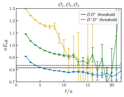
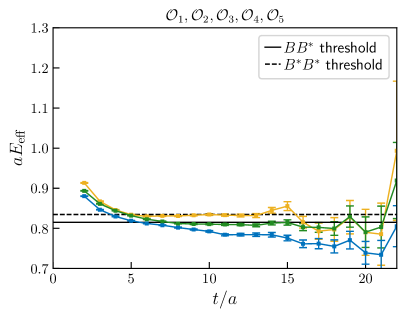
Figure 1: Effective energies from a GEVP for ensemble a09m310. (left) $3\times 3$ matrix, only local interpolating operators $\mathcal{O}_{1}$, $\mathcal{O}_{2}$ and $\mathcal{O}_{3}$. (right) $5\times 5$ matrix, both local interpolating operators $\mathcal{O}_{1}$, $\mathcal{O}_{2}$ and $\mathcal{O}_{3}$ and scattering interpolating operators $\mathcal{O}_{4}$ and $\mathcal{O}_{5}$.

5 Scattering analysis

To determine the mass of the $\bar{b}\bar{b}ud$ tetraquark in infinite volume (for a given ensemble, i.e. at given $m_{\pi}$ and nonzero $a$), we proceed as in our previous work [8]:

• Compute the two lowest energy levels in the finite spatial volume (see section 4).

• Compute the corresponding phase shifts $\delta_{0}(k_{0})$, $\delta_{0}(k_{1})$ using Lüscher’s finite-volume method [17].

• Parameterize $\delta_{0}(k_{0})$, $\delta_{0}(k_{1})$ using the effective-range expansion,

  $$k\cot(\delta_{0}(k))=\frac{1}{a_{0}}+\frac{r_{0}}{2}k^{2}$$ (6)

  with fit parameters $a_{0}$ and $r_{0}$.

• The mass of the $\bar{b}\bar{b}ud$ tetraquark (and the energy of the first excitation) in infinite spatial volume corresponds to a pole in the scattering amplitude

  $$T_{0}(k)=\frac{1}{\cot(\delta_{0}(k))-i}.$$ (7)

  The position of the pole can be obtained via Eqs. (6) and (7).

The dark-gray data points in the left plot of Figure 2 represent lattice QCD finite-volume energy levels (ground state and first excitation) for three different volumes $V=L^{3}$ with $L/a=24,32,40$, but identical $a\approx 0.12\,\textrm{fm}$ and $m_{\pi}\approx 220\,\textrm{MeV}$ (ensembles a12m220S, a12m220, a12m220L). The orange curves correspond to the two lowest finite volume energy levels as functions of the spatial extent $L$, computed with Lüscher’s finite-volume method using the effective-range expansion (6). There are rather small differences between the finite-volume and infinite-volume energy levels. We attribute this to the large binding energy, $\Delta E_{0}\approx\mathcal{O}(100\,\textrm{MeV})$. Scattering analyses are, however, expected to be more important for smaller binding energies (e.g. for the $\bar{b}\bar{b}su$ system with $J^{P}=1^{+}$) and essential for tetraquark resonances (e.g. for the $\bar{b}\bar{b}ud$ system with $I(J^{P})=0(1^{-})$ [10]).

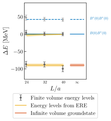
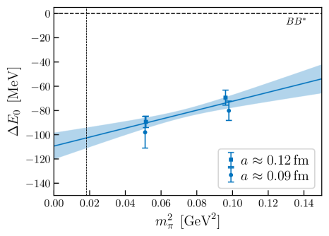
Figure 2: (left) Lattice QCD finite volume energy levels (dark gray: ground state and first excitation) for three different volumes $V=L^{3}$ with $L/a=24,32,40$, but identical $a\approx 0.12\,\textrm{fm}$ and $m_{\pi}\approx 220\,\textrm{MeV}$ (ensembles a12m220S, a12m220, a12m220L) together with a fit based on the effective range expansion (6). (right) Extrapolation of the tetraquark binding energy in the light $u/d$ quark mass to the physical point.

The right plot of Figure 2 shows an extrapolation of the tetraquark binding energy in the light $u/d$ quark mass based on the six ensembles listed in Table 1. The preliminary result at the physical pion mass $m_{\pi,\textrm{\scriptsize phys}}=135\,\textrm{MeV}$ is

$$\Delta E_{0}(m_{\pi,\textrm{\scriptsize phys}})\approx(-103\pm 8)\>\textrm{MeV},$$ (8)

where only the statistical uncertainty is shown. This binding energy is slightly smaller than, but consistent with, previous lattice results [3, 5, 6, 7, 8].

References

- [1] R. Aaij et al. [LHCb], Nature Phys. 18, no. 7, 751-754 (2022) [arXiv:2109.01038 [hep-ex]].
- [2] R. Aaij et al. [LHCb], Nature Commun. 13, no. 1, 3351 (2022) [arXiv:2109.01056 [hep-ex]].
- [3] A. Francis, R. J. Hudspith, R. Lewis and K. Maltman, Phys. Rev. Lett. 118, 142001 (2017) [arXiv:1607.05214 [hep-lat]].
- [4] A. Francis, R. J. Hudspith, R. Lewis and K. Maltman, Phys. Rev. D 99, 054505 (2019) [arXiv:1810.10550 [hep-lat]].
- [5] P. Junnarkar, N. Mathur and M. Padmanath, Phys. Rev. D 99, 034507 (2019) [arXiv:1810.12285 [hep-lat]].
- [6] R. J. Hudspith, B. Colquhoun, A. Francis, R. Lewis and K. Maltman, Phys. Rev. D 102, 114506 (2020) [arXiv:2006.14294 [hep-lat]].
- [7] P. Mohanta and S. Basak, Phys. Rev. D 102, 094516 (2020) [arXiv:2008.11146 [hep-lat]].
- [8] L. Leskovec, S. Meinel, M. Pflaumer and M. Wagner, Phys. Rev. D 100, 014503 (2019) [arXiv:1904.04197 [hep-lat]].
- [9] S. Meinel, M. Pflaumer and M. Wagner, Phys. Rev. D 106, 034507 (2022) [arXiv:2205.13982 [hep-lat]].
- [10] J. Hoffmann, A. Zimermmane-Santos, M. Pflaumer, M. Wagner, poster at LATTICE2022.
- [11] A. Bazavov et al. [MILC], Phys. Rev. D 87, 054505 (2013) [arXiv:1212.4768 [hep-lat]].
- [12] T. Bhattacharya et al. [PNDME], Phys. Rev. D 92, 094511 (2015) [arXiv:1506.06411 [hep-lat]].
- [13] R. Gupta, Y. C. Jang, B. Yoon, H. W. Lin, V. Cirigliano and T. Bhattacharya, Phys. Rev. D 98, 034503 (2018) [arXiv:1806.09006 [hep-lat]].
- [14] R. J. Dowdall et al. [HPQCD], Phys. Rev. D 85, 054509 (2012) [arXiv:1110.6887 [hep-lat]].
- [15] A. Abdel-Rehim, C. Alexandrou, J. Berlin, M. Dalla Brida, J. Finkenrath and M. Wagner, Comput. Phys. Commun. 220, 97-121 (2017) [arXiv:1701.07228 [hep-lat]].
- [16] C. Alexandrou, T. Leontiou, C. N. Papanicolas and E. Stiliaris, Phys. Rev. D 91, 014506 (2015) [arXiv:1411.6765 [hep-lat]].
- [17] M. Lüscher, Nucl. Phys. B 354, 531-578 (1991).