Unifying Graph Contrastive Learning
with Flexible Contextual Scopes

Abstract

Graph contrastive learning (GCL) has recently emerged as an effective learning paradigm to alleviate the reliance on labelling information for graph representation learning. The core of GCL is to maximise the mutual information between the representation of a node and its contextual representation (i.e., the corresponding instance with similar semantic information) summarised from the contextual scope (e.g., the whole graph or 1-hop neighbourhood). This scheme distils valuable self-supervision signals for GCL training. However, existing GCL methods still suffer from limitations, such as the incapacity or inconvenience in choosing a suitable contextual scope for different datasets and building biased contrastiveness. To address aforementioned problems, we present a simple self-supervised learning method termed Unifying Graph Contrastive Learning with Flexible Contextual Scopes (UGCL for short). Our algorithm builds flexible contextual representations with tunable contextual scopes by controlling the power of an adjacency matrix. Additionally, our method ensures contrastiveness is built within connected components to reduce the bias of contextual representations. Based on representations from both local and contextual scopes, UGCL optimises a very simple contrastive loss function for graph representation learning. Essentially, the architecture of UGCL can be considered as a general framework to unify existing GCL methods. We have conducted intensive experiments and achieved new state-of-the-art performance in six out of eight benchmark datasets compared with self-supervised graph representation learning baselines. Our code has been open sourced.

I Introduction

Graph neural networks (GNNs) employ a neighbourhood aggregation strategy via iterative message passing to learn low-dimensional node embeddings for permutation-invariant graphs. GNNs have achieved promising results in various graph-based tasks such as node classification [1, 2], link prediction [3], and graph classification [4]. They have been further applied to address various real-world problems such as anomaly detection [5], graph similarity computation [6], time series forcasting [7, 8] and trustworthy systems [9, 10].

The majority of GNNs learn node representations following (semi-)supervised paradigms where supervision signals are provided from manual labels. However, in the real world, collecting labels is an expensive and labour-intensive process. To address this problem, graph contrastive learning (GCL) methods are produced to alleviate the reliance on labels in graph representation learning [11, 12, 13, 14, 15, 16, 17]. The key idea of GCL methods is to maximise the mutual information (MI) between the representation of a node and its contextual representation (i.e., the corresponding node instance with similar semantic information) summarised from the contextual scope (e.g., 1-hop neighbourhood). In particular, aiming to extract global semantic information, global contrasting methods such as DGI [11] and MVGRL [13] contrast nodes with a readout graph embedding. Focusing on localised information, localised contrasting methods (e.g., GRACE [14], and GMI [12]) maximise MI between a node and its close neighbourhood or augmented counterpart.

Though GCL methods can reduce the reliance on labelling information during training, they still share the following deficiencies: 1) the establishment of the contextual representation requires a contextual scope, while the size of this scope is hard to adjust; 2) the aggregated contextual representation is biased in existing GCL methods, as they neglect the independence of connected components.

The first limitation arises since most GCL methods only have contextual representations generated from a fixed scope. However, with different properties (e.g., type of edges and sparsity), datasets from various domains (e.g., citation networks and social networks) can have different suitable contextual scopes. For example, in social networks, a faraway neighbour can be semantically unrelated based on the theory of six degrees of separation [18], as all people are no more than six-hop away from each other. However, a remote neighbour can still be similar to a target node in citation networks since they share the same research field. In addition, the sparsity of graphs can affect the contextual scope since a sparse graph may need a larger receptive field to include sufficient informative neighbours. Therefore, selecting a suitable contextual scope for different datasets is necessary. We have provided theoretical justification for why different graphs require different contextual scope in Section IV-C. However, with a fixed scope, existing GCL methods cannot well exploit supervision signals from the suitable scale for different datasets.

For the second limitation, some GCL methods (e.g., DGI [11] and MVGRL [13]) build contrastiveness between a node and a whole graph, neglecting the fact that many graphs in practice are composed of many independent connected components (as shown in Figure 1). In general, node embedding generation within a connected component will not be affected by other components. Thus, different connected components ought to have their own contextual representations and can be different from each other. In this case, contrasting to a whole graph can be biased as it neglects this independence and mixes up representations from different components, which impairs the model ability to explore fine-grained information within each connected component.

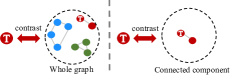
Figure 1: “T” is the target node, and the red arrow means contrastiveness. The left part shows contrastiveness between “T” and a whole graph, while the right part is contrastiveness built within a connected component.

To alleviate the aforementioned problems in GCL, we propose a new method termed Unifying Graph Contrastive Learning with Flexible Contextual Scopes (namely UGCL). The theme of our algorithm is to establish contextual representations by tuning the power of an adjacency matrix, which flexibly expands the contextual scope based on node proximity. This mechanism can be regarded as the aggregation which summarises the information embodied in a selected scale. Based on this idea, UGCL can generate contextual representations from a suitable scale for different datasets. Additionally, as graph convolution is only effective on connected components when generating contextual representations, UGCL considers the independence of connected components and reduces the bias of the generated representations by building contrastiveness within a connected component as shown in the right part of Figure 1.

Benefits. UGCL is conceptually simple, easy to implement, and nicely addresses limitations of common GCL approaches. In particular, it can tune contextual scope easily and ensure contrastiveness is conducted within connected components to reduce bias of contextual representations. More significantly, the architecture of UGCL is a general framework that unifies representative GCL approaches, including localised contrasting methods and global contrasting methods.

II Preliminary

II-A Problem Definition

In this paper, we focus on unsupervised node representation learning problem. Given an attributed graph $\mathcal{G=(\textbf{X},\textbf{A})}$, where $\textbf{X}\in\mathbb{R}^{N\times D}$ is feature matrix and $\textbf{A}\in\mathbb{R}^{N\times N}$ denotes the adjacency matrix, we aim to learn a GNN encoder $g(\cdot)$ to generate node representations without the guidance of labels. Here, $N$ is the number of nodes in $\mathcal{G}$, $D$ is the feature dimension. The output representation, i.e., $\textbf{H}=g(\textbf{X},\textbf{A})\in\mathbb{R}^{N\times D^{\prime}}$, where $D^{\prime}$ is the hidden embeddings dimension. H can be utilised for various downstream tasks, such as node classification and link prediction.

II-B Representations Convergence with Raising Power Theorem

Theorem 1 (Representations Convergence with Raising Power Theorem).

Given an adjacency matrix A, when $n$ increases, multiplying with the $n$-th power of A, node representations H within a connected component will gradually converge to a shared subspace $\mathcal{M}$ as shown below:

$$\rm d_{\mathcal{M}}(\textbf{A}^{n}\textbf{H})\leq\lambda d_{\mathcal{M}}(\textbf{A}^{n-1}\textbf{H}),$$ (1)

where the definition of subspace $\mathcal{M}$ and the distance of graph representation to $\mathcal{M}$ (i.e., $d_{\mathcal{M}}$), are defined in Appendix. $\lambda$ is the second largest eigenvalue of A. The computation of $\textbf{A}^{n}$ is formulated as $\textbf{A}^{n}=\underbrace{\textbf{A}\textbf{A}\cdots\textbf{A}}_{n}$.

This theorem shows that as $n$ increases, node representations will converge to a subspace $\mathcal{M}$ as $\lambda$ is guaranteed to be smaller than 1 (as shown in Lemma 2 in Appendix). Thus, with sufficiently large $n$-th power for A, the generated contextual node representation can summarise all node embeddings within a connected components. This is because it encodes information of the whole graph. The detailed proof of this theorem is presented in Appendix.

II-C Contextual Homophily Rate & Graph Sparsity

Here, we define the contextual homophily rate $\mathcal{P}_{n}(i)$ to evaluate the homophily rate (i.e., rate of neighbours sharing the same label as the target node) in the contextual scope and graph sparsity $T_{\mathcal{G}}$.

Definition 1 (Contextual Hompohily Rate).

The contextual homophily rate of a node $i$ is $\mathcal{P}_{n}$(i), where $n$ means its contextual scope is based on $n$-th power of A (i.e., $n$-hop neighbourhood):

$$\mathcal{P}_{n}(i)=|\frac{j\in\mathcal{N}_{n}(i)\wedge y_{i}=y_{j}}{j\in\mathcal{N}_{n}(i)}|,$$ (2)

where $y$ is label for a node, and $\mathcal{N}_{n}(i)$ is the neighbourhood for node $i$ with $n$-th power of A, i.e., n-hop neighbourhood.

Definition 2 (Graph Sparsity).

The sparsity $T_{\mathcal{G}}$ of a given graph $\mathcal{G}$ is:

$$T_{\mathcal{G}}=\frac{E}{N\times N}\approx\frac{N\times d}{N\times N},$$ (3)

where $d$ is the average degree of nodes in $\mathcal{G}$, while $E$ and $N$ represent the number of edges and nodes in $\mathcal{G}$ respectively.

III Method

In this section, we introduce the proposed UGCL which learns node representations via the power adjustment of A in a self-supervised fashion. The overall architecture of our method is illustrated in Figure 2. To train our model, we first create two views: patch- and contextual view, where the latter view is generated with the $n$-th power of A. Then, we construct a cross-view contrastiveness in a pair-wise contextual relationship between these two views. The following sections illustrate the details of view establishment and the cross-view contrastiveness of UGCL.

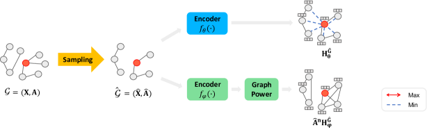
Figure 2: The overall architecture of UGCL. Firstly, we conduct subsampling on $\mathcal{G}=(\textbf{X},\textbf{A})$ to construct its subgraph $\hat{\mathcal{G}}$, whose size is predefined by a parameter $S$, Then, $\hat{\mathcal{G}}$ is fed into two GNN-based encoders, the primary encoder $f_{\theta}(\cdot)$ and the auxiliary encoder $f_{\varphi}(\cdot)$, to generates node representations $\textbf{H}^{\hat{\mathcal{G}}}_{\theta}$, and $\textbf{H}^{\hat{\mathcal{G}}}_{\varphi}$, respectively. After that, $\textbf{H}^{\hat{\mathcal{G}}}_{\varphi}$ is multiplied with $n$-th power of $\hat{\textbf{A}}$ to obtain contextual representations. Finally, a contrastive learning scheme is deployed, where the red solid line indicates MI maximisation, while multiple blue dash lines represent the opposite operation.

III-A View Establishment

In our method, the view establishment process generates two views (i.e., patch view and contextual view), based on which a cross-view contrastive learning scheme is employed to compute contrastive loss. As shown in Figure 2, a subgraph $\hat{\mathcal{G}}=(\hat{\textbf{X}},\hat{\textbf{A}})$ is sampled from $\mathcal{G}$ and fed into two GNN encoders, the main encoder $f_{\theta}(\cdot)$ and the auxiliary encoder $f_{\varphi}(\cdot)$, to get two variants of node representations $\textbf{H}^{\hat{\mathcal{G}}}_{\theta}$ and $\textbf{H}^{\hat{\mathcal{G}}}_{\varphi}$ for $\hat{\mathcal{G}}$. In our experiment, we adopt a one-layer GCN as the GNN encoder. The details of the subsampling process is presented in the subsection below. Here, we consider $\textbf{H}^{\hat{\mathcal{G}}}_{\theta}$ as the patch view representation. To obtain the contextual view representation, we first compute the $n$-th power of $\hat{\textbf{A}}$ and multiply the output with $\textbf{H}^{\hat{\mathcal{G}}}_{\varphi}$. This process can be formulated as follows:

$$\tilde{\textbf{H}}^{\hat{G}}_{\varphi}=\hat{\textbf{A}}^{n}\textbf{H}^{\hat{G}}_{\varphi},$$ (4)

where $\tilde{\textbf{H}}^{\hat{\mathcal{G}}}_{\varphi}$ is the contextual view representation, and $n$ is a tunable parameter. It is worth noting that the computation of $\hat{\textbf{A}}^{n}$ can be easily relieved with sub-sampling and matrix multiplication decomposition. The computation time of this power mechanism is less than or around 1 millisecond for five datasets of various sizes (as shown in Table LABEL:graph_power). In our proposed method, $n$ is a key parameter to control the contextual scope of contextual representation $\tilde{\textbf{H}}^{\hat{\mathcal{G}}}_{\varphi}$. As the $n$-th power of A gives the number of paths of length $n$ between two nodes, two vertices are adjacent if the distance between these two vertices is less than or equal to $n$ [19]. Therefore, by multiplying $\hat{\textbf{A}}^{n}$ with $\textbf{H}^{\hat{\mathcal{G}}}_{\varphi}$, the contextual scope of contextual representations can be extended to $n$-hop neighbourhood.

Subsampling. We adopt a very simple yet effective subsampling process for data augmentation. Specifically, we randomly pick a preset number of nodes and their edges to form a subgraph for training in each training epoch. The advantages of this approach are two folds: preserving essential properties (i.e., the sparsity $T_{\mathcal{G}}$ and the contextual homophily rate of $\textbf{A}^{1}$, $\mathcal{P}_{1}(i)$) of the given graph $\mathcal{G}$, and building diversified subgraphs with trivial computation and sufficient randomness.

To prove the first advantage, we propose the following proposition:

Proposition 1.

Given a Graph $\mathcal{G}$ with $d$ average node degree and $\mathcal{P}_{1}(i)$ homophily rate for the first power of A, its sampled graph $\hat{\mathcal{G}}$ still have similar sparsity $T_{\hat{\mathcal{G}}}$ and $\mathcal{P}_{1}(i)$ as $\mathcal{G}$.

Proof.

As the sparsity of $\mathcal{G}$, $T_{\mathcal{G}}$, equals to $\frac{E}{N\times N}$ and $E\approx N\times d$, we can derive that $T_{\mathcal{G}}\approx\frac{N\times d}{N\times N}=\frac{d}{N}$. After sampling, we can obtain a subgraph $\hat{\mathcal{G}}$, which has $S$ nodes. For each node, it would have $S\times d\times\frac{S}{N}$ neighbours, i.e., edges. Thus, the sparsity of the subgraph $\hat{\mathcal{G}}$, $T_{\hat{\mathcal{G}}}\approx\frac{S\times d\times\frac{S}{N}}{S\times S}=\frac{d}{N}$. As $T_{\mathcal{G}}$ is approximately equal to $T_{\hat{\mathcal{G}}}$, we show that the sparsity of $\mathcal{G}$ and $\hat{\mathcal{G}}$ is similar. In addition, as edges in $\hat{\mathcal{G}}$ come from the original graph $\mathcal{G}$, they still connect approximately the same ratio ($\mathcal{P}_{1}(i)$) of homophilic neighbours (i.e., nodes sharing the same label as $i$). Here, we prove the above proposition. ∎

The second advantage alleviates the reliance on the fixed graph during model training. As we sample a subgraph in each training epoch, the sampled subgraph is changing instead of in the static state. As a result, the model has to be versatile to handle the contrastiveness built with changing topology. This can be regarded as an augmentation to increase the difficulty of the self-supervised pre-text tasks, which may improve the model performance. We have conducted an ablation study in Section VI-C to show its effectiveness.

III-B Cross-View Contrastive Learning

In UGCL, the cross-view contrastive learning scheme consists of two contrastive paths, which are the patch-view contrastive path and the cross-view contrastive path. In the same view, the first path distinguishes an anchor node embedding from other node embeddings, which are considered negative samples. The latter path simply maximises the cosine similarity between a patch view representation and its corresponding contextual representation (i.e., positive samples). By combining both paths, we can form the contrastive learning objective.

As shown in Figure 2, after processing $\hat{\mathcal{G}}$ into the primary GNN encoder $f_{\theta}(\cdot)$, we can get the patch view representation $\textbf{H}^{\hat{\mathcal{G}}}_{\theta}$. Within the patch view, giving the set of nodes $V$ in $\hat{\mathcal{G}}$ and an anchor node $v\in V$, we define that all nodes except for the anchor node as negative samples to regularise the contrastive loss via MI minimisation. In addition, we define an anchor node representation in the patch view $h_{v}\in\textbf{H}^{\hat{\mathcal{G}}}_{\theta}$ and contextual view $\tilde{h}_{v}\in\tilde{\textbf{H}}^{\hat{\mathcal{G}}}_{\varphi}$ as the positive pair (red line in Figure 2). By discriminating representations in the positive pair, our model can distil self-supervision signals from the chosen contextual scope. The contrastive loss function can be formulated as follows:

$$\mathcal{L}=-\frac{1}{S}\sum^{S}_{v\in V}\log\frac{e^{\cos(\textit{h}_{v},\tilde{\textit{h}}_{v})}}{\sum^{N}_{u\in V;u\neq v}e^{\cos(\textit{h}_{v},\textit{h}_{u})}},$$ (5)

where $\cos(\cdot)$ is the cosine similarity function, $S$ represents the number of nodes in the sampled graph, $h_{v}$ and $\tilde{h}_{v}$ denote the anchor node patch- and contextual representation respectively.

III-C Model Training

To train our model end-to-end, we leverage the loss $\mathcal{L}$ defined in Equation (5). The training objective is to minimise $\mathcal{L}$ during the optimisation. To obtain the output embeddings for downstream tasks, we first generate $\textbf{H}^{\mathcal{G}}_{\theta}$ with the trained GNN encoder $g_{\theta}$ and $\tilde{\textbf{H}}^{\mathcal{G}}_{\theta}$ by multiplying $\textbf{H}^{\mathcal{G}}_{\theta}$ with $\textbf{A}^{n}$. Finally, we aggregate these two representations: $\textbf{H}=\textbf{H}^{\mathcal{G}}_{\theta}+\tilde{\textbf{H}}^{\mathcal{G}}_{\theta}$ to get the final representations.

IV Unifying Representative GCL Methods

To learn node representations in a self-supervised manner, GCL methods usually inject contrastiveness between patch view and contextual view [20]. In Figure 3, we present the general architecture of UGCL, which can be considered as a unified framework of GCL methods. From the framework, GCL generally follows three steps: augmentation, graph encoding and contrasting. Specifically, the optional first step is applying augmentation to the original graph $\mathcal{G}=(\textbf{X},\textbf{A})$ to create semantically similar graph instances $\hat{\mathcal{G}}$. In UGCL, we regard subsampling as augmentation. Then, the graph encoder $g(\cdot)$ generates node representations $\textbf{H}^{\hat{\mathcal{G}}}_{g}=g(\hat{\mathcal{G}})$. To train $g(\cdot)$, contrastiveness is built between node representations and their corresponding contextual representations to acquire self-supervision signals via MI maximisation:

$$g^{*}(\cdot)=\mathop{\arg\max}\limits_{g}\textbf{MI}(\textbf{H}^{\hat{\mathcal{G}}}_{g},\textbf{A}^{n}\textbf{H}^{\hat{\mathcal{G}}}_{g}),\vspace{-2mm}$$ (6)

where $g^{*}(\cdot)$ is the trained encoder, $\textbf{MI}(\cdot)$ is a mutual information neural estimator [21] consisting of discriminative network (i.e., bilinear transformation or cosine similarity) and contrastive loss, $\textbf{H}^{\hat{\mathcal{G}}}_{g}$ and $\textbf{A}^{n}\textbf{H}^{\hat{\mathcal{G}}}_{g}$ represent node- and contextual representations respectively. In the following sections, we interprets four representative GCL methods of two categories (i.e., localised- and global contrasting methods) with the proposed unified framework.

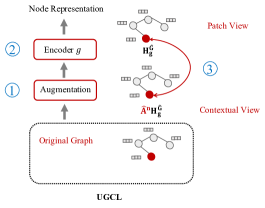
Figure 3: A unified framework for GCL methods. The red line indicates contrastiveness.

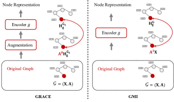
(a) Localised contrasting methods

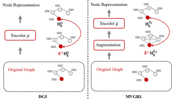
(b) Global contrasting methods

Figure 4: (a) Localised contrasting methods interpreted with the architecture of UGCL. (b) Global contrasting methods interpreted with the architecture of UGCL.

IV-A Connections to Localised Contrasting Methods

Localised contrasting methods form pretext tasks by pulling the representation of a node closer to its augmented counterpart or close neighbours to distil the localised contextual information [14, 12, 15]. These methods can be considered as UGCL with a tiny $n$ for the power of A when building the contextual view. To illustrate this point, we present GRACE [14] and GMI [12] (i.e., two typical localised methods) with the unified framework in Figure 4(a).

In particular, GRACE can be considered as contrasting a node to a contextual representation with 0-th power, i.e., $\textbf{A}^{0}=\textbf{I}$. It employs two different graph augmentation methods to generate two augmented views $\hat{\mathcal{G}}_{1}$ and $\hat{\mathcal{G}}_{2}$, where it pulls the representations of the same node in these two views closer. This node-to-node comparison strategy allows GRACE to extract the most fine-grained information from the contextual scope with only one node (i.e., a node’s augmented counterpart). This scheme is equal to applying $\textbf{A}^{0}$ to the generated contextual representation, as we only care about the semantic information embodied within a node itself:

$$g^{*}(\cdot)=\underset{g}{\rm arg\ max}\operatorname{\textbf{MI}}\left(\textbf{H}_{g}^{\hat{\mathcal{G}}_{1}},\textbf{A}^{0}\textbf{H}_{g}^{\hat{\mathcal{G}}_{2}}\right).\vspace{-2mm}$$ (7)

Different from GRACE, GMI extends the contextual scope to 1-hop neighbourhood. It maximises the MI between a node and the raw features of its 1-hop neighbours. This is similar to contrasting the raw features X with 1-th power of A, which aggregates a node 1-hop neighbourhood:

$$g^{*}(\cdot)=\underset{g}{{\rm arg\ max}}\operatorname{\textbf{MI}}\left(\textbf{H}_{g}^{\mathcal{G}},\textbf{A}^{1}\textbf{X}\right).\vspace{-2mm}$$ (8)

This contextual representation can provide the very-local information of a node for contrastiveness. However, focusing only on the close neighbourhood, these localised methods neglect useful information from a broader receptive field.

IV-B Connections to Global Contrasting Methods

Global contrasting methods place discrimination between a node and a graph-level embedding, summarising all node representations in a graph [13, 11]. In a special case (i.e., the input graph only has one connected component), these approaches are similar to UGCL with infinite power for A. The interpretation of DGI and MVGRL in the architecture of UGCL is presented in Figure 4(b). DGI aims to extract global semantic information from graph-level embedding. Specifically, they create the graph-level embedding by coarsely averaging all node embeddings in a graph. MVGRL extends DGI with additional augmentation, which creates two augmented views $\hat{\mathcal{G}}_{1}$ and $\hat{\mathcal{G}}_{2}$.

Similarly, we can also apply the infinite power of A to generate graph-level contextual representations. According to Theorem 1, with the infinite power of A, node representations within a connected component become similar and converge to a certain point or shared subspace. This is because nodes iteratively receive messages from all other nodes within the same connected component, which smooths the difference between these nodes. Thus, the oversmoothed representations can be regarded as the graph-level embedding in the aforementioned special case (i.e., the input graph only has one connected component). These global contrasting methods can be approximated by applying infinite power of A to the contextual view in UGCL:

$$g^{*}(\cdot)=\underset{g}{\rm arg\ max}\operatorname{\textbf{MI}}(\textbf{H}_{g}^{\mathcal{G}},\textbf{A}^{\infty}\textbf{H}^{\mathcal{G}}_{g}),$$ (9)

$$g^{*}(\cdot)=\underset{g}{\rm arg\ max}\operatorname{\textbf{MI}}(\textbf{H}_{g}^{\hat{\mathcal{G}}_{1}},\textbf{A}^{\infty}\textbf{H}_{g}^{\hat{{\mathcal{G}}_{2}}}),\vspace{-2mm}$$ (10)

where Equation (9) and Equation (10) are formulas for DGI and MVGRL in the unified framework. Though these global contrasting methods can extract supervision signals from the global view, with the largest contextual scope, it is inevitable to include irrelevant noise and impede the model training.

IV-C Theoretical Justification for Flexible Contextual Scope

Here, we provide theoretical justification for why different graphs require different contextual scope from the perspective of homophily dominance [22]. Moreover, based on this theoretical analysis, we can guide the selection of $n$-th power for A in model training.

Existing GNNs assume homophily in prior graphs to be effective. To obtain effective representations, nodes in the contextual scope are expected to be homophily dominant[22], which can be achieved when $\mathcal{P}_{n}(i)$ is at least larger than any $\{|\frac{j\in\mathcal{N}_{n}(i)\wedge y_{j}\in c}{j\in\mathcal{N}_{n}(i)}|;c\in C\}$, where $C$ is number of classes for the graph. Here we consider $i$ as a node with the average degree of $\mathcal{G}$, $d$, and assume $\mathcal{P}_{1}(i)$ equals to the homophily rate of a graph, i.e., the proportion of edges connecting same class nodes. To hold homophily dominance, $\mathcal{P}_{n}(i)$ needs to be as large as possible. The following lemma shows the lower bound of $\mathcal{P}_{n}(i)$ is determined by $\mathcal{P}_{1}(i)$ and $d$:

Lemma 1.

Given $\mathcal{G}$ with an average degree of $d\geq 1$ for each node and contextual homophily rate with 1-th power $\mathcal{P}_{1}(i)$. With $n$-th power of A, the lower bound of $\mathcal{P}_{n}(i)$ is:

$$\mathcal{P}_{n}(i)>\frac{(d-1)\mathcal{P}_{1}(i)(d^{n}\mathcal{P}_{1}^{n}(i)-1)}{(d^{n}-1)(d\mathcal{P}_{1}(i)-1)}.\vspace{-6mm}$$ (11)

Based on Lemma 11 and Definition 2, we can derive four properties:

Property 1.

Given a graph $\mathcal{G}$, when $n$ increases, the lower bound of $\mathcal{P}_{n}(i)$ drops.

Property 2.

Given a graph $\mathcal{G}$, when $\mathcal{P}_{1}(i)$ increases, the lower bound of $\mathcal{P}_{n}(i)$ increases.

Property 3.

Given a graph $\mathcal{G}$, when $d$ increases, the lower bound of $\mathcal{P}_{n}(i)$ drops.

Property 4.

Given a graph $\mathcal{G}$, when $T_{\mathcal{G}}$ increases, the lower bound of $\mathcal{P}_{n}(i)$ drops.

Property 2, Property 3 and Property 4 indicate the choice of $n$ is closely related to two essential properties of graphs, i.e., sparsity and homophily. Specifically, when a graph is dense (i.e., the sparsity $T_{\mathcal{G}}$ is large), a large $n$ can easily break the homophily dominance and degrade model performance. In addition, under the same level of sparsity, a low $n$ is preferable for a low $\mathcal{P}_{1}(i)$, i.e., homophily rate. These findings are consistent with our experiment results shown in Section VI-D1. The detailed proof of Lemma 11, Properties 1-4 are provided as follows:

Proof.

Give a graph $\mathcal{G}$ with an average degree of $d$ for each node and homophily rate with 1-th power of A, $\mathcal{P}_{1}(i)$. $d$, $\mathcal{P}_{1}(i)$ and $n$ are all positive numbers. With $d$, the total number of nodes in the neighbourhood for $n$-th power of A is equal to $d+d^{2}+\cdots+d^{n}$. For the number of homophilic nodes in the neighbourhood, we know it is at least $d\mathcal{P}_{1}(i)$ for the first-hop neighbourhood, $d^{2}\mathcal{P}_{1}(i)^{2}$ for the second-hop neighbourhood, and so on. Thus, the lower bound of this number is equal to $d\mathcal{P}_{1}(i)+d^{2}\mathcal{P}_{1}(i)^{2}+\cdots+d^{n}\mathcal{P}_{1}(i)^{n}$. Here, we can formulate the lower bound of $\mathcal{P}_{n}(i)$ as:

$$\mathcal{P}_{n}(i) >\frac{\sum_{k=1}^{n}d^{k}\mathcal{P}_{1}(i)^{k}}{\sum_{k=1}^{n}d^{k}}$$ (12)

$$=\frac{(d-1)\mathcal{P}_{1}\left(d^{n}\mathcal{P}_{1}(i)^{n}-1\right)}{\left(d^{n}-1\right)(d\mathcal{P}_{1}(i)-1)}.$$

From the above formula, we first prove Property 1. The gap between denominator and numerator of the lower bound of $\mathcal{P}_{n}(i)$ would become larger when $n$ increases. This is because when $n$ increases by 1, the numerator would increase $d^{n}\mathcal{P}_{1}(i)^{n}$, while the denominator would increase $d^{n}$. It is easy to observe the gap between $d^{n}\mathcal{P}_{1}(i)^{n}$ and $d^{n}$ would become larger and larger when $n$ increases as $0<\mathcal{P}_{1}(i)<1$. Thus, we prove that when $n$ increases, the lower bound of $\mathcal{P}_{n}(i)$ drops.

To prove Property 2, we present the partial derivative with respect to $\mathcal{P}_{1}(i)$ for the numerator of the lower bound of $\mathcal{P}_{n}(i)$:

$$f^{\mathcal{P}_{n}(i)}_{num} =\sum_{k=1}^{n}d^{k}\mathcal{P}_{1}(i)^{k},$$ (13)

$$\frac{\partial f^{\mathcal{P}_{n}(i)}_{num}}{\partial\mathcal{P}_{1}(i)} =d+2d^{2}\mathcal{P}_{1}(i)+3d^{3}\mathcal{P}_{1}(i)^{2}+\cdots+nd^{n}\mathcal{P}_{1}(i)^{n-1},$$

where $f^{\mathcal{P}_{n}(i)}_{num}$ is the numerator for $\mathcal{P}_{n}(i)$. As $d\geq 1$ and $\mathcal{P}_{1}>0$, $\frac{\partial f^{\mathcal{P}_{n}(i)}_{num}}{\partial\mathcal{P}_{1}(i)}$ is a positive number. In addition, changing $\mathcal{P}_{1}(i)$ will not affect the denominator of the lower bound of $\mathcal{P}_{n}(i)$. Thus, we can derive that increasing $\mathcal{P}_{1}(i)$ will lead to the monotonical increase for the lower bound of $\mathcal{P}_{n}(i)$ and prove Property 2.

From Equation 12, we can also prove Property 3 as follows:

$$\mathcal{P}_{n}(i) >\frac{\sum_{k=1}^{n}d^{k}\mathcal{P}_{1}(i)^{k}}{\sum_{k=1}^{n}d^{k}}$$ (14)

$$=\sum^{n}_{k=1}(\frac{d^{k}}{\sum^{n}_{k=1}d^{k}})\mathcal{P}_{1}(i)^{k},$$

here we define $\frac{d^{k}}{\sum^{n}_{k=1}d^{k}}$ as $M$, then we can obtain the derivative of $M$:

$$\frac{dM}{dd} =\sum^{n}_{k=1}\frac{d^{k-1}(\sum^{n}_{k=1}d^{k})-d^{k}(\sum^{n}_{k=1}kd^{k-1})}{(\sum^{n}_{k=1}d^{k})^{2}}$$ (15)

$$=\frac{\sum_{k=1}^{n}d^{2k-1}-\sum_{k=1}^{n}kd^{2k-1}}{(\sum^{n}_{k=1}d^{k})^{2}}$$

$$=\frac{\sum_{k-1}^{n}d^{2k-1}-\sum_{k=1}^{n}kd^{2k-1}}{(\sum^{n}_{k=1}d^{k})^{2}}$$

$$=\frac{\sum_{k=1}^{n}(1-k)d^{2k-1}}{(\sum^{n}_{k=1}d^{k})^{2}}$$

$$=\frac{\sum^{n}_{k=2}(1-k)d^{2k-1}}{(\sum^{n}_{k=1}d^{k})^{2}}<0.$$

From the derivative of $M$, we can see the increase of $d$ (i.e., increasing sparsity $T_{\mathcal{G}}$) leads to the monotonical decrease of $M$, which causes the drop of the lower bound of $\mathcal{P}_{n}(i)$. Thus, we prove Property 3 and 4.

∎

Though different graphs require different contextual scope, aforementioned GCL methods only have fixed contextual scope. In contrast, UGCL can adjust the contextual scope by changing $n$, which allows us to choose the most suitable scale for datasets with different properties. Moreover, we can select $n$ guiding by the theoretical findings above.

IV-D Guidance of Selecting $n$

We consider the $n$ just before the break of strong homophily dominance (i.e., $\mathcal{P}_{n}(i)>0.5$) as the selected $n$ for model training. Homophily-dominant neighbourhoods are more beneficial for GNN layers, since in such neighbourhoods the class label of each node may be determined by the majority of the class labels in the neighbourhood [22]. However, only meeting the homophily-dominant requirement may not be sufficient for generating high quality contextual representation. This is because homophily-dominant neighbourhood can still include too much abundant or noisy neighbouring information, i.e., neighbouring nodes with different classes. To ensure the neighbourhood aggregation is conducted with a majority of homophilic neighbours, we consider the break of strong homophily dominance as the condition to select $n$. Surprisingly, this approach provides a good guidance to the selection of $n$. The $n$ just before the break of strong homophily dominance of $\mathcal{P}_{n}(i)$ is consistent with the best $n$ for 4 out of 5 datasets. The experiment result is presented in Section VI-D1.

V Related Work

V-A Graph Neural Networks

Firstly introduced in Scarselli’s work [23], GNNs aim to extend deep neural networks to handle graph-structured data. GNNs consist of two domains: spectral-based methods [24, 25, 26, 27] and spatial-based methods [28, 29, 30]. While spectral-based methods adopt spectral representation of graphs, spatial-based methods conduct feature aggregation based on nodes spatial neighbours (e.g., GAT [28]). Notably, GCN [28] bridges the gap between these two domains by approximating spectral-based convolution with the first order of Chebyshev polynomial filters. Spatial-based methods are currently more prosperous since they have advantages in efficiency and general applicability. For example, to further improve GCN, GAT [28] presents an attention-based approach to weightly aggregate node neighbours representations. SGC [31] simplifies GCN by removing the non-linearity and collapsing weight matrices among graph convolution layers. However, most GNNs rely extensively on labelling information, whereas the collecting process is expensive. To address this issue, GCL emerged. We proposed UGCL, which can generate effective node representations without labelling information.

V-B Contrastive Learning

Contrastive learning is a self-supervised learning paradigm usually based on MI maximisation. It aims to maximise MI between similar data instances (e.g., the same object in different augmented views and representations of the same object in different scales) [20, 32]. It has been successfully applied in image classification tasks with promising results. For example, Deep Infomax [33], Moco [34], and SimCLR [31] train image encoders by discriminating two augmented images. Recently, some works attempted to adapt this concept to GNNs. DGI [11] borrows the MI maximisation idea from Deep Infomax [33] and builds contrastiveness by contrasting node- and graph-level contextual representations. MVGRL [13] further enriches the contrastiveness by building contrastiveness between augmented views of graphs.

Different from DGI and MVGRL, GRACE [14] and GMI [12] create contextual representation from the same scale, first-order neighbourhood, respectively. Though these GCL methods have achieved promising results, they still share several issues, including the fixed contextual scope and biased contextual representation. UGCL addresses these problems as it can easily adjust the contextual scope and ensure contrastiveness is built within connected components.

VI Experiment

TABLE I: Node classification results on 7 small to medium-sized datasets compared with 14 baselines. Here, the “Data” column indicates what kind of data the method need to use in training. X, A and Y means feature matrix, adjacency matrix, and label information, respectively. OOM represents out-of-memory. The best performance for each dataset is in bold.

Data	Method	Cora	CiteSeer	PubMed	Coauthor Physics	Coauthor CS	Amazon Computers	Amazon Photos
X, A, Y	MLP	56.1$\pm{0.3}$	56.9$\pm{0.4}$	71.4$\pm{0.1}$	93.5$\pm{0.1}$	90.4$\pm{0.1}$	73.9$\pm{0.1}$	78.5$\pm{0.1}$
X, A, Y	GCN	81.5	70.3	79.0	95.7$\pm{0.2}$	93.0$\pm{0.3}$	86.3$\pm{0.5}$	87.3$\pm{1.0}$
X, A, Y	GAT	83.0$\pm{0.7}$	72.5$\pm{0.7}$	79.0$\pm{0.3}$	95.5$\pm{0.2}$	92.3$\pm{0.2}$	87.1$\pm{0.4}$	86.2$\pm{1.5}$
X, A, Y	SGC	81.0$\pm{0.0}$	71.9$\pm{0.1}$	78.9$\pm{0.0}$	95.8$\pm{0.1}$	92.7$\pm{0.1}$	74.4$\pm{0.1}$	86.4$\pm{0.0}$
X, A	DeepWalk	69.5$\pm{0.6}$	58.8$\pm{0.6}$	69.9$\pm{1.3}$	91.8$\pm{0.2}$	84.6$\pm{0.2}$	85.7$\pm{0.1}$	89.4$\pm{0.1}$
X, A	Node2vec	71.2$\pm{1.0}$	47.6$\pm{0.8}$	66.5$\pm{1.0}$	91.2$\pm{0.1}$	85.1$\pm{0.1}$	84.4$\pm{0.1}$	89.7$\pm{0.1}$
X, A	GAE	71.1$\pm{0.4}$	65.2$\pm{0.4}$	71.7$\pm{0.9}$	94.9$\pm{0.1}$	90.0$\pm{0.7}$	85.3$\pm{0.2}$	91.6$\pm{0.1}$
X, A	VGAE	79.8$\pm{0.9}$	66.8$\pm{0.4}$	77.2$\pm{0.3}$	94.5$\pm{0.1}$	92.1$\pm{0.1}$	86.4$\pm{0.2}$	92.2$\pm{0.1}$
X, A	DGI	81.7$\pm{0.6}$	71.5$\pm{0.7}$	77.3$\pm{0.6}$	94.5$\pm{0.5}$	92.2$\pm{0.6}$	84.1$\pm{0.4}$	91.5$\pm{0.3}$
X, A	GMI	82.7$\pm{0.2}$	73.0$\pm{0.3}$	80.1$\pm{0.2}$	OOM	OOM	76.8$\pm{0.1}$	85.1$\pm{0.1}$
X, A	MVGRL	82.9$\pm{0.7}$	72.6$\pm{0.7}$	79.4$\pm{0.3}$	95.3$\pm{0.1}$	92.1$\pm{0.1}$	81.8$\pm{0.5}$	90.7$\pm{0.3}$
X, A	GRACE	80.0$\pm{0.4}$	71.7$\pm{0.6}$	79.5$\pm{1.1}$	OOM	92.8$\pm{0.1}$	87.2$\pm{0.4}$	92.7$\pm{0.3}$
X, A	GCA	80.4$\pm{0.4}$	71.2$\pm{0.2}$	80.4$\pm{0.8}$	95.9$\pm{0.2}$	93.3$\pm{0.1}$	87.8$\pm{0.3}$	93.2$\pm{0.3}$
X, A	BGRL	81.1$\pm{0.2}$	71.6$\pm{0.4}$	80.0$\pm{0.4}$	95.8$\pm{0.4}$	93.3$\pm{0.4}$	88.9$\pm{0.3}$	93.2$\pm{0.3}$
X, A	UGCL	84.7$\pm{0.3}$	74.1$\pm{0.2}$	81.6$\pm{0.3}$	95.6$\pm{0.3}$	93.4$\pm{0.3}$	90.1$\pm{0.5}$	93.8$\pm{0.7}$

TABLE II: The statistics of benchmark datasets.

Dataset	Nodes	Edges	Features	Classes
Cora	2,708	5,429	1,433	7
CiteSeer	3,327	4,732	3,703	6
PubMed	19,717	44,338	500	3
Coauthor CS	18,333	81,894	6,805	15
Coauthor Physics	34,493	991,848	8,415	5
Amazon Computers	13,752	245,861	767	10
Amazon Photos	7,650	119,081	745	8
ogbn-arxiv	169,343	1,166,243	128	40

TABLE III: Node classification result on ogbn-arxiv.

Method	Valid	Test
MLP	57.7$\pm{0.4}$	55.5$\pm{0.2}$
Supervised GCN	73.0$\pm{0.2}$	71.7$\pm{0.3}$
Node2vec	71.3$\pm{0.1}$	70.1$\pm{0.1}$
DGI	71.3$\pm{0.1}$	70.3$\pm{0.2}$
GRACE	72.6$\pm{0.2}$	71.5$\pm{0.1}$
BGRL	72.5$\pm{2.1}$	71.6$\pm{1.6}$
UGCL	72.6$\pm{0.4}$	71.4$\pm{0.6}$

VI-A Details of the Experiments

To evaluate the effectiveness of our proposed method, we conducted extensive experiments on 8 benchmark datasets, including 5 citation networks (i.e., Cora, CiteSeer, PubMed, Coauthor CS, and Physics), 2 Amazon co-purchasing networks (i.e., Amazon Computers and Photos), and a large-scale dataset, ogbn-arxiv. The statistic of these datasets is summarised in Table II. For the first three networks, we adopt the same dataset split as [35]. For Coauthor and Amazon datasets, we randomly split these datasets, where 10%, 10% and the remaining nodes are chosen for training, validation and test set, respectively. For the large-scale dataset, ogbn-arxiv, we use the default setting as described in [36].

In our experiment, we mainly tune three parameters: $n$-th power of A , sample size $S$, and hidden size $D^{\prime}$. Specifically, $n$ is selected from 1 to 20, while $S$ is chosen from 500 to 3000, with every increment by 500, for Cora and Citeseer, and 3000 to 10000, with every increment by 1000, for the remaining datasets. For $D^{\prime}$, it is chosen from {512, 1024, 2048, 4196, 8192}. After tunning these parameters, the best performance of our model for each dataset is recorded in Table I.

TABLE IV: The evaluation of $n$-th power of A on five benchmark datasets. $\mathcal{P}_{n}(i)$ is the contextual homophily rate for each $n$. The best performance for each dataset is in bold. The $n$ and the model performance just before the break of homophily dominance according to $\mathcal{P}_{n}(i)$ are underlined. “Homo rate” means the proportion of homophily edges, which connect nodes with the same class, on total number of edges in the graph. It equals to $\mathcal{P}_{1}(i)$.

Dataset	Sparsity $T_{\mathcal{G}}$	Homo Rate $\mathcal{P}_{1}(i)$	1	2	3	4	5	6	7	8	9	10
Cora	0.074%	81.0%	80.1$\pm{0.2}$	82.0$\pm{0.1}$	83.2$\pm{0.2}$	83.9$\pm{0.3}$	84.2$\pm{0.2}$	84.3$\pm{0.4}$	84.4$\pm{0.3}$	84.6$\pm{0.4}$	84.7$\pm{\textbf{0.3}}$	83.8$\pm{0.4}$
$\mathcal{P}_{n}(i)^{cora}$	-	-	0.81	0.75	0.67	0.59	0.52	0.45	0.39	0.34	0.29	0.25
CiteSeer	0.042%	72.6%	74.0$\pm{0.2}$	74.1$\pm{\textbf{0.2}}$	73.9$\pm{0.3}$	73.7$\pm{0.3}$	73.8$\pm{0.4}$	73.7$\pm{0.2}$	73.7$\pm{0.3}$	73.7$\pm{0.2}$	73.6$\pm{0.3}$	73.5$\pm{0.2}$
$\mathcal{P}_{n}(i)^{citeseer}$	-	-	0.73	0.6	0.48	0.38	0.3	0.23	0.17	0.13	0.1	0.07
PubMed	0.011%	80.2%	76.6$\pm{0.4}$	78.6$\pm{0.3}$	79.4$\pm{0.4}$	80.1$\pm{0.4}$	80.4$\pm{0.2}$	80.4$\pm{0.4}$	79.8$\pm{0.3}$	81.3$\pm{0.2}$	81.3$\pm{0.1}$	81.4$\pm{\textbf{0.2}}$
$\mathcal{P}_{n}(i)^{pubmed}$	-	-	0.80	0.73	0.68	0.63	0.59	0.56	0.54	0.52	0.51	0.50
Amazon Computers	0.130%	77.7%	89.9$\pm{0.5}$	90.1$\pm{\textbf{0.8}}$	89.1$\pm{1.1}$	89.4$\pm{1.0}$	89.3$\pm{1.1}$	87.7$\pm{0.7}$	87.4$\pm{1.2}$	87.1$\pm{0.9}$	87.0$\pm{0.8}$	87.2$\pm{0.9}$
$\mathcal{P}_{n}(i)^{ac}$	-	-	0.78	0.62	0.48	0.37	0.29	0.23	0.18	0.14	0.11	0.08
Amazon Photos	0.203%	82.7%	92.5$\pm{0.6}$	93.4$\pm{0.4}$	93.8$\pm{\textbf{0.4}}$	93.4$\pm{0.3}$	93.0$\pm{0.9}$	92.9$\pm{0.5}$	92.9$\pm{1.3}$	92.0$\pm{1.5}$	92.3$\pm{1.2}$	91.6$\pm{0.6}$
$\mathcal{P}_{n}(i)^{ap}$	-	-	0.83	0.71	0.59	0.49	0.4	0.33	0.28	0.23	0.19	0.16

VI-B Node Classification Results

We choose 14 baselines to be compared with UGCL on node classification tasks. These baselines consist of MLP and three types of GNNs: supervised-, conventional self-supervised, and GCL approaches. For supervised GNNs, we select three widely-adopted supervised GNNs, which are GCN [27], GAT [28], SGC [30]. Four conventional self-supervised methods including DeepWalk [37], Node2vec [38], GAE [39] and VGAE [39], and six GCL methods including DGI [11], GMI  [12], MVGRL [13], GRACE [14], GCA [40], and BGRL [41] are chosen to be compared with our model.

We run all baselines and our model on each small to medium-sized dataset five times, and the average node classification accuracy and associated standard deviation are reported in Table I. The table shows that UGCL  achieved the best performance on 6 out of 7 small to medium-sized datasets. Notably, UGCL surpasses its self-supervised counterparts by 2.1% in Cora, 1.1% in CiteSeer, and 1.2% in Amazon Computers.

In addition, we compare UGCL with supervised methods (i.e., MLP and Supervised GCN) and self-supervised methods, including Node2vec, DGI, GRACE, and BGRL on ogbn-arxiv. The other GCL methods are not selected as they encounter out-of-memory issue during training. The experiment results are presented in Table III, where we can observe UGCL has achieved on-par performance with the most competitive baselines (i.e., GRACE and BGRL). Except for UGCL, others results in the table are sourced from  [41]

UGCL generally achieves promising results on benchmark datasets because with $n$-th power of A, UGCL  can tune the contextual scope while most GCL baselines can only contrast to a fixed scope. Additionally, UGCL ensures the contrastiveness is established within connected components to reduce the bias of contextual representations. These advantages allow UGCL to focus on the suitable scale and lead to model performance improvement.

TABLE V: Ablation study of UGCL.

Method	Cora	Citeseer	Pubmed
$\textbf{{UGCL}}_{\rm mean}$	79.1$\pm{0.5}$	70.5$\pm{0.5}$	77.2$\pm{0.5}$
$\textbf{{UGCL}}_{\rm smooth}$	81.3$\pm{0.5}$	71.9$\pm{0.5}$	80.8$\pm{0.5}$
$\textbf{{UGCL}}_{\rm sig}$	84.2$\pm{0.3}$	72.2$\pm{0.4}$	81.1$\pm{0.2}$
$\textbf{{UGCL}}_{\rm w/o\ sam}$	84.1$\pm{0.5}$	73.2$\pm{0.4}$	80.8$\pm{1.0}$
$\textbf{{UGCL}}_{\rm w/o\ p}$	80.8$\pm{0.6}$	71.4$\pm{0.2}$	79.5$\pm{0.4}$
UGCL	84.7$\pm{0.3}$	74.1$\pm{0.2}$	81.6$\pm{0.3}$

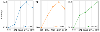
Figure 5: Parameter analysis for hidden size $D$ on Cora, CiteSeer, and PubMed.

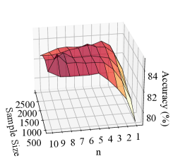
(a) Cora

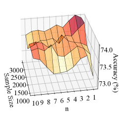
(b) CiteSeer

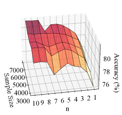
(c) PubMed

Figure 6: Joint parameter analysis of sample size and $n$-th power of A.

VI-C Ablation Study

In this section, we compare the performance of our original method to its five variants: $\texttt{UGCL}_{\rm mean}$, $\texttt{UGCL}_{\rm smooth}$, $\texttt{UGCL}_{\rm sig}$, $\texttt{UGCL}_{\rm sam}$, and $\texttt{UGCL}_{\rm w/o\ p}$ on Cora, CiteSeer, and PubMed. The comparative results have been exhibited in Table V.

For $\texttt{UGCL}_{\rm mean}$, the graph-level embedding is generated with the naive mean pooling approach, whereas $\texttt{UGCL}_{\rm smooth}$ uses 100-th power of A to obtain oversmoothed embeddings which summarise all nodes information within a connected component. The method $\texttt{UGCL}_{\rm smooth}$ consistently outperforms $\texttt{UGCL}_{\rm mean}$, which indicates that establishing the contrastiveness within connected components instead of the whole graph is effective.

$\texttt{UGCL}_{\rm sig}$ uses a single encoder for both local and contextual view establishment, while UGCL utilizes an additional auxiliary encoder for generating the contextual view. This auxiliary encoder targets to embed contextual information for better contextual representations generation. $\texttt{UGCL}_{\rm w/o\ sam}$ have no subsampling, while UGCL uses subsampling as an augmentation to both increase the difficulty of the contrastive learning tasks and extend the scalability. $\texttt{UGCL}_{\rm w/o\ p}$ removes the power mechanism for the contextual view, whereas UGCL employs this mechanism to control the contextual scope of contextual representations. To shed light on the contributions of the auxiliary GNN encoder, subsampling, and the power mechanism, we compare UGCL with $\texttt{UGCL}_{\rm w/o\ sam}$, $\texttt{UGCL}_{\rm sig}$, and $\texttt{UGCL}_{\rm w/o\ p}$ on three benchmark datasets. It is apparent that the model performance degrades without any of the three mechanisms mentioned above, which validates the effectiveness of these mechanisms.

VI-D Parameter Study

VI-D1 n-th power of A

$n$ is a key parameter used to choose the $n$-th power of A for contextual view generation. To evaluate the effect of $n$, we run UGCL with $n$ ranging from 1 to 10. Based on Equation 11, we can calculate the lower bound of $\mathcal{P}_{n}(i)$ for each $n$ with $d$ and $\mathcal{P}_{1}(i)$. Here, we assume $\mathcal{P}_{1}(i)$ equals to the homophily rate of the dataset.

The model performance and the value of $\mathcal{P}_{n}(i)$ on 5 datasets are reported in Table IV. Here, we adopt the best parameter settings for each dataset except for $n$. Specifically, the chosen sample size $S$ are 1000, 3000, 7000, 10000, and 5000 for Cora, CiteSeer, PubMed, Computers and Photos, respectively. As shown in the underlined results in Table IV, we can see the $n$ just before the break of strong homophily dominance (i.e., $\mathcal{P}_{n}(i)>0.5$) for the lower bound of $\mathcal{P}_{n}(i)$ is consistent with the best $n$ for 4 out of 5 datasets. Though for Cora, the selected $n$ is not optimal, it still achieves state-of-the-art performance (84.2%) compared with baselines.

VI-D2 Hidden Size $D^{\prime}$

Hidden size $D^{\prime}$ controls the dimensionality of hidden layers in the GNN encoder, and we change $D^{\prime}$ from 512 to 8192 to see its effect on the model performance. The experiment results of the parameter analysis are shown in Figure 5. The model performance on a larger dataset (i.e., PubMed) grows consistently when $D^{\prime}$ increases, whereas the other two datasets achieve the highest performance at first and then degrade. We conjecture this is because a large $D^{\prime}$ with too many parameters may overfit on small datasets.

VI-D3 Joint Influence of Sample Size $S$ and $n$

In this section, we explore the joint influence of sample sizes $S$ and $n$ on three datasets: Cora, CiteSeer, and PubMed. Specifically, we choose $S$ ranging from 500 to 2500 for Cora, 1000 to 3000 for CiteSeer with every increment by 500, and 3000 to 7000 for PubMed with every increment by 1000. The experiment result is presented in Figure 6. For Cora and CiteSeer, we can observe that when $S$ increases, the model performance peaks at lower $n$. For PubMed, the model performance all peaks when $n$ is 10.

This experiment result is consistent with our theoretical findings in Section IV-C. We conjecture this phenomenon is because when $S$ increases, the average node degree $d$ would increase for the generated subgraph $\hat{\mathcal{G}}$ as the average node degree in $\hat{\mathcal{G}}$ is $\frac{S}{N}d$. According to Property 3, when $d$ increases, the lower bound of $\mathcal{P}_{n}$ drops and leads to the break of homophily dominance easily when $n$ increases. Thus, the optimal $n$ decreases with the growth of $S$. For PubMed, from Table IV, we can see even with 7000 for $S$, the homophily dominance still holds when $n$ is 10. Thus, it is reasonable that the model performance all peaks at $n=10$.

TABLE VI: $n$-th power of A computation time in seconds on five datasets. Number in bracket means the number of $n$ used for the dataset.

Cora(7)	CiteSeer(6)	PubMed(10)	Computers(1)	Photos(2)
2.6e-04	2.2e-04	3.7e-04	2.7e-04	1.3e-03

VI-E Computation for $n$-th Power of A

To show the easiness of the computation for $n$-th Power of A in UGCL, we run experiments on five datasets (i.e., Cora, CiteSeer, PubMed, Amazon Computers, and Amazon Photos) and report the average computation time per epoch in seconds for this operation in Table LABEL:graph_power. From the table, we can observe that the computation is trivial in the training process.

VII Conclusion

In this paper, we propose a novel GCL approach, namely UGCL. We design a cross-scale contrastiveness to fuel the GNN encoder learning process by discriminating node representations in the patch- and contextual view. The proposed power mechanism allows our method to adjust the contextual scope when building contrastiveness and ensures the contrastiveness is established within connected components. These advantages allow UGCL  to conduct a more fine-grained contrastiveness than the naive pooling approach and reduce the bias of generated contextual representations. Moreover, the architecture of UGCL  can be considered as a unified framework to interpret existing GCL methods. Extensive experiments validate the effectiveness of our proposed approach in node classification tasks.

Appendix A Proof of Theorem 1.

We first provide the Lemma 2, the definition of subspace, and Lemma 3:

Lemma 2.

Given an adjacency matrix A, its normalized augmented adjacency is ${\hat{\textbf{A}}=\hat{\textbf{D}}^{-\frac{1}{2}}(\textbf{A}+\textbf{I})\hat{\textbf{D}}^{-\frac{1}{2}}}$, where ${\hat{\textbf{D}}=\textbf{D}+\textbf{I}}$, and I is the identity matrix. ${\hat{\textbf{A}}}$ is symmetric with real eigenvalues $\lambda_{1}\leq\lambda_{2}\leq...\lambda_{N}$, which have been sorted ascendingly. If the algebraic multiplicity of the largest eigenvalue $\lambda_{N}$ is $K\leq N$, which means the top $K$ eigenvalue are the same, we have the following properties:

• $\lambda_{N-K+1},\lambda_{N-K+2}\cdots\lambda_{N}$ = 1, i.e., the $K$ largest eigenvalue equals to 1;

• $\lambda_{N-K}<1;\lambda_{1}>-1$, i.e., the second largest eigenvalue is smaller than 1, while the smallest eigenvalue is larger than -1;

• The multiplicity $K$ is the number of connected components in the Graph $\mathcal{G}$ with the adjacency matrix A. For each connected component, we have the eigenvector $\hat{v}_{k}:={\hat{\textbf{D}}^{\frac{1}{2}}u_{k}}$ corresponding to the eigenvalue $\lambda_{N-K}$, where $u_{k}\in\mathbb{R}^{N}$ indicates whether a node is belong to the $K$-th component.

Definition 3 (Subspace).

We define the subspace $\mathcal{M}\in\mathbb{R}^{N\times D}$ by $\mathcal{M}:=\{{\textbf{H}\in\mathbb{R}^{N\times D}|\textbf{H}=\hat{\textbf{V}}\textbf{M},\textbf{M}\in\mathbb{R}^{K\times D}\}}$, where ${\hat{\textbf{V}}\in\mathbb{R}^{N\times K}}$ is a collection of eigenvectors $\hat{v}_{k}$ of the largest eigenvalue of ${\hat{\textbf{A}}}$ in Theorem 1.

Lemma 3.

Given a normalized adjacency matrix ${\hat{\textbf{A}}\in\mathbb{R}^{N\times N}}$, a feature matrix ${\textbf{H}\in\mathbb{R}^{N\times D}}$, the projection matrix for $\mathcal{M}$, ${\hat{\textbf{V}}\hat{\textbf{V}}^{T}}$ , where ${\hat{\textbf{V}}}$ is the normalized bases of $\mathcal{M}$, and ${\hat{\textbf{F}}}$ is the orthogonal complement of ${\hat{\textbf{V}}}$, we have:

$${d_{\mathcal{M}}(\textbf{H})} ={\parallel\hat{\textbf{F}}^{T}\textbf{H}\parallel_{F}},$$ (16)

$${d_{\mathcal{M}}(\hat{\textbf{A}}\textbf{H})} ={\parallel\Lambda\hat{\textbf{F}}^{T}\textbf{H}\parallel_{F}},$$

$$\leq{\parallel\Lambda\parallel_{F}\parallel\hat{\textbf{F}}^{T}\textbf{H}\parallel_{F}},$$

where $d_{\mathcal{M}}(\cdot)$ is the distance between representations and the subspace $\mathcal{M}$. The distance between node representations H and $\mathcal{M}$ is denoted as $d_{\mathcal{M}}({\textbf{H}})=\rm inf_{p\in\mathcal{M}}\parallel\textbf{H}-p\parallel_{F}$. $\Lambda$ denotes all eigenvalues excluding the $K$ largest eigenvalues, and $\parallel\cdot\parallel_{F}$ represents the Frobenius norm.

Proof.

Lemma 2 has been proved by [42] to show augmented spectral property of an augmented adjacency, while Lemma 2 has been proved by [43] based on the notion of projection. A projection matrix can project a given vector or matrix onto subspace to obtain the projected vector or matrix. By utilising Equation (16) in Lemma 3, we will have the following derivation:

$$d_{\mathcal{M}}(\hat{\textbf{A}}^{n}\textbf{H}) =\parallel\Lambda^{n}\hat{\textbf{F}}^{T}\textbf{H}\parallel_{F},$$ (17)

$$=\parallel\Lambda\Lambda^{n-1}\hat{\textbf{F}}^{T}\textbf{H}\parallel_{F},$$

$$\leq\parallel\Lambda\parallel_{F}\parallel\Lambda^{n-1}\hat{\textbf{F}}^{T}\textbf{H}\parallel_{F},$$

$$\leq\parallel\Lambda\parallel_{F}d_{\mathcal{M}}(\hat{\textbf{A}}^{n-1}\textbf{H}),$$

$$\leq\lambda d_{\mathcal{M}}(\hat{\textbf{A}}^{n-1}\textbf{H}).$$

Here, we get the inequality shown in Theorem 1.

∎

References

- [1] M. Jin, Y. Zheng, Y.-F. Li, C. Gong, C. Zhou, and S. Pan, “Multi-scale contrastive siamese networks for self-supervised graph representation learning,” IJCAI, 2021.
- [2] Y. Liu, Y. Zheng, D. Zhang, H. Chen, H. Peng, and S. Pan, “Towards unsupervised deep graph structure learning,” in WWW, 2022.
- [3] M. Zhang and Y. Chen, “Link prediction based on graph neural networks,” NIPS, vol. 31, pp. 5165–5175, 2018.
- [4] M. Zhang, Z. Cui, M. Neumann, and Y. Chen, “An end-to-end deep learning architecture for graph classification,” in AAAI, 2018.
- [5] Y. Liu, Z. Li, S. Pan, C. Gong, C. Zhou, and G. Karypis, “Anomaly detection on attributed networks via contrastive self-supervised learning,” TNNLS, 2021.
- [6] D. Jin, L. Wang, Y. Zheng, X. Li, F. Jiang, W. Lin, and S. Pan, “Cgmn: A contrastive graph matching network for self-supervised graph similarity learning,” IJCAI, 2022.
- [7] M. Jin, Y. Zheng, Y.-F. Li, S. Chen, B. Yang, and S. Pan, “Multivariate time series forecasting with dynamic graph neural odes,” arXiv preprint arXiv:2202.08408, 2022.
- [8] M. Jin, Y.-F. Li, and S. Pan, “Neural temporal walks: Motif-aware representation learning on continuous-time dynamic graphs,” in NIPS, 2022.
- [9] H. Zhang, B. Wu, X. Yuan, S. Pan, H. Tong, and J. Pei, “Trustworthy graph neural networks: Aspects, methods and trends,” arXiv preprint arXiv:2205.07424, 2022.
- [10] H. Zhang, B. Wu, X. Yang, C. Zhou, S. Wang, X. Yuan, and S. Pan, “Projective ranking: A transferable evasion attack method on graph neural networks,” in CIKM, 2021.
- [11] P. Veličković, W. Fedus, W. L. Hamilton, P. Liò, Y. Bengio, and R. D. Hjelm, “Deep graph infomax,” ICLR, 2019.
- [12] Z. Peng, W. Huang, M. Luo, Q. Zheng, Y. Rong, T. Xu, and J. Huang, “Graph representation learning via graphical mutual information maximization,” in WWW, 2020, pp. 259–270.
- [13] K. Hassani and A. H. Khasahmadi, “Contrastive multi-view representation learning on graphs,” in ICML. PMLR, 2020, pp. 4116–4126.
- [14] Y. Zhu, Y. Xu, F. Yu, Q. Liu, S. Wu, and L. Wang, “Deep graph contrastive representation learning,” arXiv preprint arXiv:2006.04131, 2020.
- [15] Y. Jiao, Y. Xiong, J. Zhang, Y. Zhang, T. Zhang, and Y. Zhu, “Sub-graph contrast for scalable self-supervised graph representation learning,” in ICDM. IEEE, 2020, pp. 222–231.
- [16] Y. Zheng, M. Jin, S. Pan, Y.-F. Li, H. Peng, M. Li, and Z. Li, “Towards graph self-supervised learning with contrastive adjusted zooming,” arXiv preprint arXiv:2111.10698, 2021.
- [17] Y. Zheng, S. Pan, V. C. Lee, Y. Zheng, and P. S. Yu, “Rethinking and scaling up graph contrastive learning: An extremely efficient approach with group discrimination,” NIPS, 2022.
- [18] S. Milgram, “The small world problem,” Psychology today, vol. 2, no. 1, pp. 60–67, 1967.
- [19] R. Balakrishnan and K. Ranganathan, A textbook of graph theory. Springer Science & Business Media, 2012.
- [20] Y. Liu, M. Jin, S. Pan, C. Zhou, Y. Zheng, F. Xia, and P. Yu, “Graph self-supervised learning: A survey,” TKDE, 2022.
- [21] M. I. Belghazi, A. Baratin, S. Rajeshwar, S. Ozair, Y. Bengio, A. Courville, and D. Hjelm, “Mutual information neural estimation,” in ICML. PMLR, 2018, pp. 531–540.
- [22] J. Zhu, Y. Yan, L. Zhao, M. Heimann, L. Akoglu, and D. Koutra, “Beyond homophily in graph neural networks: Current limitations and effective designs,” NIPS, 2020.
- [23] F. Scarselli, M. Gori, A. C. Tsoi, M. Hagenbuchner, and G. Monfardini, “The graph neural network model,” TNNLS, 2008.
- [24] M. Defferrard, X. Bresson, and P. Vandergheynst, “Convolutional neural networks on graphs with fast localized spectral filtering,” NIPS, 2016.
- [25] M. Henaff, J. Bruna, and Y. LeCun, “Deep convolutional networks on graph-structured data,” arXiv preprint arXiv:1506.05163, 2015.
- [26] J. Bruna, W. Zaremba, A. Szlam, and Y. LeCun, “Spectral networks and locally connected networks on graphs,” ICLR, 2013.
- [27] T. N. Kipf and M. Welling, “Semi-supervised classification with graph convolutional networks,” ICLR, 2016.
- [28] P. Veličković, G. Cucurull, A. Casanova, A. Romero, P. Lio, and Y. Bengio, “Graph attention networks,” ICLR, 2017.
- [29] W. L. Hamilton, R. Ying, and J. Leskovec, “Inductive representation learning on large graphs,” in NIPS, 2017.
- [30] F. Wu, A. Souza, T. Zhang, C. Fifty, T. Yu, and K. Weinberger, “Simplifying graph convolutional networks,” in ICML, 2019.
- [31] T. Chen, S. Kornblith, M. Norouzi, and G. Hinton, “A simple framework for contrastive learning of visual representations,” in ICML, 2020.
- [32] Y. Tan, G. Long, J. Ma, L. Liu, T. Zhou, and J. Jiang, “Federated learning from pre-trained models: A contrastive learning approach,” in First Workshop on Pre-training: Perspectives, Pitfalls, and Paths Forward at ICML 2022.
- [33] R. D. Hjelm, A. Fedorov, S. Lavoie-Marchildon, K. Grewal, P. Bachman, A. Trischler, and Y. Bengio, “Learning deep representations by mutual information estimation and maximization,” ICLR, 2019.
- [34] K. He, H. Fan, Y. Wu, S. Xie, and R. Girshick, “Momentum contrast for unsupervised visual representation learning,” in CVPR, 2020.
- [35] Z. Yang, W. Cohen, and R. Salakhudinov, “Revisiting semi-supervised learning with graph embeddings,” in ICML. PMLR, 2016, pp. 40–48.
- [36] W. Hu, M. Fey, M. Zitnik, Y. Dong, H. Ren, B. Liu, M. Catasta, and J. Leskovec, “Open graph benchmark: Datasets for machine learning on graphs,” arXiv preprint arXiv:2005.00687, 2020.
- [37] B. Perozzi, R. Al-Rfou, and S. Skiena, “Deepwalk: Online learning of social representations,” in KDD, 2014.
- [38] A. Grover and J. Leskovec, “node2vec: Scalable feature learning for networks,” in KDD, 2016.
- [39] T. N. Kipf and M. Welling, “Variational graph auto-encoders,” arXiv preprint arXiv:1611.07308, 2016.
- [40] Y. Zhu, Y. Xu, F. Yu, Q. Liu, S. Wu, and L. Wang, “Graph contrastive learning with adaptive augmentation,” in WWW, 2021.
- [41] S. Thakoor, C. Tallec, M. G. Azar, M. Azabou, E. L. Dyer, R. Munos, P. Veličković, and M. Valko, “Large-scale representation learning on graphs via bootstrapping,” ICLR, 2022.
- [42] K. Oono and T. Suzuki, “Graph neural networks exponentially lose expressive power for node classification,” ICLR, 2020.
- [43] W. Huang, Y. Rong, T. Xu, F. Sun, and J. Huang, “Tackling over-smoothing for general graph convolutional networks,” TPAMI, 2020.