Positive-Unlabeled Learning using Random Forests via Recursive Greedy Risk Minimization

Abstract

The need to learn from positive and unlabeled data, or PU learning, arises in many applications and has attracted increasing interest. While random forests are known to perform well on many tasks with positive and negative data, recent PU algorithms are generally based on deep neural networks, and the potential of tree-based PU learning is under-explored. In this paper, we propose new random forest algorithms for PU-learning. Key to our approach is a new interpretation of decision tree algorithms for positive and negative data as recursive greedy risk minimization algorithms. We extend this perspective to the PU setting to develop new decision tree learning algorithms that directly minimizes PU-data based estimators for the expected risk. This allows us to develop an efficient PU random forest algorithm, PU extra trees. Our approach features three desirable properties: it is robust to the choice of the loss function in the sense that various loss functions lead to the same decision trees; it requires little hyperparameter tuning as compared to neural network based PU learning; it supports a feature importance that directly measures a feature’s contribution to risk minimization. Our algorithms demonstrate strong performance on several datasets. Our code is available at https://github.com/puetpaper/PUExtraTrees.

1 Introduction

Positive and unlabeled learning (PU learning) has attracted increasing interest recently, due to its broad applications, including disease gene identification [24], landslide susceptibility modeling [29], inference of transcriptional regulatory network [23], cybersecurity [30] and many others [2].

Existing algorithms generally reduce PU learning to solving one or more supervised learning problems. A naive approach is to simply learn a classifier by treating all unlabeled examples as negative, but unlabeled examples can be either positive or negative. Various approaches have been developed to better handle the uncertainty on the labels of the unlabeled examples. A common approach follows an iterative two-step learning process: the first step identifies reliable negative examples, then the second step learns a model using the positive examples, the reliable negative examples and possibly unlabeled examples [22, 15]. Another common approach transforms the PU dataset into a weighted fully labeled dataset [20, 12, 11, 16]. The transformed dataset is often constructed so that the empirical risk on the transformed dataset provides a good estimate of the true risk. Depending on the assumptions on how PU data is generated, different transformations have been developed.

While random forests are known to perform well for many supervised learning problems and in principle tree-based learning methods can be applied in the above approaches, little work has been done to explore the potential of tree-based methods for PU learning. On the other hand, current state-of-the-art PU learning methods are often based on deep neural networks [16, 6]. This is partly due to the recent advances of deep learning, which allows training of powerful neural network models with relatively little effort. In addition, while it is easy to train a neural network to minimize different loss functions, it is not clear how this can be done for tree-based methods (without overfitting the dataset), because existing tree-based methods have not been designed to directly minimize the loss. In particular, it is not clear how this can be done for nonstandard risk estimators such as the non-negative PU risk (nnPU), which has already been observed to work well with neural networks [16].

We fill this gap by providing a theoretically justified approach, which we call recursive greedy risk minimization, to learn random forests from PU data in this paper. Our contributions are as follows

• A new interpretation to existing decision tree learning algorithm that links the impurity reduction based learning algorithms to empirical risk minimization.

• Efficient new decision tree and random forest algorithms that directly minimize PU-data based estimators for the expected risk.

• Our approach has three desirable properties: it is robust to the choice of the loss function in the sense that various loss functions lead to the same decision trees; it requires little hyperparameter tuning as compared to neural network based PU learning; it supports a feature importance that directly measures a feature’s contribution to risk minimization.

• Our algorithms demonstrate strong performance on several datasets.

We briefly review decision tree learning and PU learning in Section 2, introduce our recursive greedy risk minimization approach for decision tree learning in Section 3 and the PU version of extra trees in Section 4, present experiment results in Section 5, discuss related works in Section 6, and conclude in Section 7.

2 Background

Decision tree learning from positive and negative data

A decision tree is generally constructed by recursively partitioning the training set so that we can quickly obtain subsets which are more or less in the same class.

1 Notations: $\kappa$ - node; $S$ - dataset; $f$ - feature; $t$ - threshold;

2 if termination criterion is met  then

3       Compute the prediction value at $\kappa$ using $S$;

4else

5       Choose an optimal split $(f,t)$;

6       Create two child nodes $\kappa_{f>t}$ and $\kappa_{f\leq t}$ for $\kappa$;

7       $\texttt{LearnDT}(\kappa_{f>t},S_{f>t})$;

8       $\texttt{LearnDT}(\kappa_{f\leq t},S_{f\leq t})$;

9 end if

Algorithm 1 LearnDT($\kappa,S$)

Algorithm 1 shows a generic decision tree learning algorithm. We start with a single node associated with the entire set of training examples. When we encounter a node $\kappa$ associated with a set $S$ of training examples, we compute the prediction value at $\kappa$ if the termination criterion is met. If not, we first compute an optimal split $(f,t)$ for the dataset $S$, where a split $(f,t)$ tests whether a feature $f$ is larger than a value $t$, and the quality of a split is usually measured by its impurity reduction. Based on the test’s outcome, we create two child nodes $\kappa_{f>t}$ and $\kappa_{f\leq t}$, split $S$ into two subsets $S_{f>t}$ and $S_{f\leq t}$, and finally continue the learning process with $(\kappa_{f>t},S_{f>t})$ and $(\kappa_{f\leq t},S_{f\leq t})$.

Given an impurity measure $\text{Impurity}(S)$, a split $(f,t)$’s impurity reduction is

$${\rm IR}(f,t;S){\coloneqq}\text{Impurity}(S)-\frac{|S_{f>t}|}{|S|}\text{Impurity}(S_{f>t})-\frac{|S_{f\leq t}|}{|S|}\text{Impurity}(S_{f\leq t}).$$ (1)

Typically, the Gini impurity $G(S)$ and the entropy $H(S)$ are used as the impurity measure:

$$G(S) {\coloneqq}1-q_{+}^{2}-q_{-}^{2}=2q_{+}(1-q_{+}), H(S) {\coloneqq}-q_{+}\ln q_{+}-q_{-}\ln q_{-},$$ (2)

where $q_{+}$ and $q_{-}$ are the proportions of positive and negative examples in $S$ respectively.

We will use ${\rm IR}_{\text{Gini}}(f,t;S)$ and ${\rm IR}_{\text{entropy}}(f,t;S)$ to denote the impurity reduction when using the Gini impurity and the entropy impurity respectively.

PU learning

We assume that the input ${\bm{x}}\in{\mathbb{R}}^{d}$ and label $y\in\{-1,+1\}$ follow an unknown joint distribution $p({\bm{x}},y)=p({\bm{x}}\,|\,y)\,p(y)$. In the fully supervised case, the training data is generally assumed to be independently sampled from $p({\bm{x}},y)$. In the PU setting, one common assumption on the data generation mechanism [11, 10, 16] is that the positive examples $P=\{{\bm{x}}_{i}^{(\mathsf{p})}\}_{i=1}^{n_{\mathsf{p}}}$ are sampled independently from the P marginal $p_{\mathsf{p}}({\bm{x}}){\coloneqq}p({\bm{x}}\,|\,y=1)$, and the unlabeled examples $U=\{{{\bm{x}}}_{i}^{(\mathsf{u})}\}_{i=1}^{n_{\mathsf{u}}}$ are sampled independently from the marginal $p({\bm{x}})=p({\bm{x}},+1)+p({\bm{x}},-1)$. Clearly, we have $p({\bm{x}})=\pi\,p_{\mathsf{p}}({\bm{x}})+(1-\pi)\,p_{\mathsf{n}}({\bm{x}})$, where $\pi{\coloneqq}p(y=+1)$ is the positive rate and $p_{\mathsf{n}}({\bm{x}}){\coloneqq}p({\bm{x}}\,|\,y=-1)$ is the N marginal.

The objective is to learn a score function $g:{\mathbb{R}}^{d}\to{\mathbb{R}}$ (which corresponds to a classifier that outputs $+1$ iff $g({\bm{x}})>0$) such that it minimizes its expected risk

$$R(g) {\coloneqq}{\mathbb{E}}_{({\bm{x}},y)\sim p({\bm{x}},y)}\,\ell(g({\bm{x}}),y),$$ (3)

where $\ell:{\mathbb{R}}\times\{-1,+1\}\to{\mathbb{R}}$ is a loss function that gives the loss $\ell(v,y)$ incurred by predicting a score $v$ when the true label is $y$. We focus on the quadratic loss $\ell_{\text{quad}}(v,y)=(1-vy)^{2}$ , the logistic loss $\ell_{\text{logistic}}(v,y)=\ln(1+\exp(-vy))$ , the savage loss $\ell_{\text{savage}}(v,y)=4/(1+\exp({vy}))^{2}$ and the sigmoid loss $\ell_{\text{sigmoid}}(v,y)=1/(1+\exp(vy))$ in this paper.

The risk can be written in terms of positive and unlabeled data as [11]

$$R(g) =\pi\,{\mathbb{E}}_{{\bm{x}}\sim p_{\mathsf{p}}({\bm{x}})}\,\ell(g({\bm{x}}),+1)+{\mathbb{E}}_{{\bm{x}}\sim p({\bm{x}})}\,\ell(g({\bm{x}}),-1)-\pi\,{\mathbb{E}}_{{\bm{x}}\sim p_{\mathsf{p}}({\bm{x}})}\,\ell(g({\bm{x}}),-1).$$ (4)

This gives the following unbiased PU-data based risk estimator

$$\widehat{R}_{{\rm uPU}}(g) {\coloneqq}\sum_{{\bm{x}}\in P}w_{\mathsf{p}}\ell(g({\bm{x}}),+1)-\sum_{{\bm{x}}\in P}w_{\mathsf{p}}\ell(g({\bm{x}}),-1)+\sum_{{\bm{x}}\in U}w_{\mathsf{u}}\ell(g({\bm{x}}),-1),$$ (5)

where $w_{\mathsf{p}}=\pi/n_{\mathsf{p}}$ and $w_{\mathsf{u}}=1/n_{\mathsf{u}}$.

While the uPU risk estimator is unbiased, it has a negative component that provides extra incentive for the classifier to try hard to fit to the positive examples, thus potentially making the risk negative and leading to overfitting. The non-negative risk estimator

$$\widehat{R}_{{\rm nnPU}}(g) {\coloneqq}\sum_{{\bm{x}}\in P}w_{\mathsf{p}}\ell(g({\bm{x}}),+1)+\max\left\{0,\sum_{{\bm{x}}\in U}w_{\mathsf{u}}\ell(g({\bm{x}}),-1)-\sum_{{\bm{x}}\in P}w_{\mathsf{p}}\ell(g({\bm{x}}),-1)\right\}$$ (6)

alleviates this problem by forcing the sum of the negative term and the term defined on the unlabeled data to be non-negative, as the sum acts as an estimate for risk on negative examples

3 Recursive Greedy Risk Minimization

3.1 Decision trees for positive and negative data

We first introduce our recursive greedy risk minimization approach in the fully labeled case. Consider the empirical risk of $g:{\mathbb{R}}^{d}\to{\mathbb{R}}$ on a labeled training set $D=\{({\bm{x}}_{1},y_{1}),\ldots,({\bm{x}}_{n},y_{n})\}$: $\widehat{R}(g)=\sum_{({\bm{x}},y)\in D}w\ell(g({\bm{x}}),y)$, where $w=1/|D|$. If $g$ predicts a constant $v$ on a subset $S=\{({\bm{x}},y)\}$ of the training examples, then the contribution to the total empirical risk is the partial empirical risk $\widehat{R}(v;S){\coloneqq}\sum_{({\bm{x}},y)\in S}w\ell(v,y)$. The optimal constant value prediction is $v^{*}_{S}=\mathrm{argmin}_{v\in{\mathbb{R}}}\widehat{R}^{*}(v;S)$ with a minimum partial empirical risk $\widehat{R}^{*}(S){\coloneqq}\widehat{R}^{*}(v^{*}_{S};S)$.

If we switch from a constant value prediction rule to a decision stump that uses the split $(f,t)$, then the minimum partial empirical risk for such a decision stump is $\widehat{R}^{*}(S_{f>t})+\widehat{R}^{*}(S_{f\leq t})$, thus the risk reduction for the split $(f,t)$ is

$${\rm RR}(f,t;S){\coloneqq}\widehat{R}^{*}(S)-\widehat{R}^{*}(S_{f>t})-\widehat{R}^{*}(S_{f\leq t}).$$ (7)

In the following, when we need to make the loss function explicit, we will use subscript to indicate that. For example, $\widehat{R}^{*}_{{\rm quad}}(S)$ and ${\rm RR}_{{\rm quad}}(f,t;S)$, are the minimum partial empirical risk for a constant-valued prediction on $S$ and the risk reduction for the split $(f,t)$ on $S$ when using the quadratic loss.

When we choose the $(f,t)$ with maximum risk reduction in Algorithm 1, we obtain a recursive greedy risk minimization algorithm that recursively zooms in to an input region with a constant prediction, then improves the prediction rule in a greedy manner by replacing it with the decision stump with minimal empirical risk in that region.

The first main result shows that the Gini impurity reduction and entropy reduction of a split are just scaled versions of the risk reductions when using the quadratic loss and the logistic loss respectively. This implies that the standard impurity reduction based decision learning algorithm is in fact performing recursive greedy risk minimization. All proofs are in the appendix.

[]thmpnir (a) For any $S\subseteq D$, we have $\widehat{R}^{*}_{{\rm quad}}(S)=2|S|wG(S)$. As a consequence, for any $S\subseteq D$ and any split $(f,t)$ [4],

$${\rm RR}_{{\rm quad}}(f,t;S)=2|S|w{\rm IR}_{{\rm gini}}(f,t;S).$$ (8)

(b) For any $S\subseteq D$, we have $\widehat{R}^{*}_{{\rm logistic}}(S)={|S|}wH(S)$. As a consequence, for any $S\subseteq D$ and any split $(f,t)$,

$${\rm RR}_{{\rm logistic}}(f,t;S)=|S|w{\rm IR}_{{\rm entropy}}(f,t;S).$$ (9)

3.2 Decision trees for positive and unlabeled data

We are now ready to introduce a recursive greedy risk minimization approach to PU learning. We do this by making two changes to Algorithm 1: the fully labeled dataset $S$ is replaced by a set $P^{\prime}\subseteq P$ of positive examples and a set $U^{\prime}\subseteq U$ of unlabeled examples, and the split $(f,t)$ is chosen to optimize a PU version of the risk reduction.

uPU risk reduction

We first consider the simpler case of the uPU estimator. Similarly to the fully labeled case, if $g$ predicts a constant $v$ on $P^{\prime}$ and $U^{\prime}$, then the contribution to the total empirical uPU risk is

$$\widehat{R}_{{\rm uPU}}(v;P^{\prime},U^{\prime}){\coloneqq}\sum_{{\bm{x}}\in P^{\prime}}w_{\mathsf{p}}\ell(v,+1)-\sum_{{\bm{x}}\in P^{\prime}}w_{\mathsf{p}}\ell(v,-1)+\sum_{{\bm{x}}\in U^{\prime}}w_{\mathsf{u}}\ell(v,-1).$$

The optimal constant value prediction is $v^{*}_{P^{\prime},U^{\prime}}=\mathrm{argmin}_{v\in{\mathbb{R}}}\widehat{R}^{*}_{{\rm uPU}}(v;P^{\prime},U^{\prime})$ with a minimum empirical risk $\widehat{R}^{*}_{{\rm uPU}}(P^{\prime},U^{\prime}){\coloneqq}\widehat{R}^{*}_{{\rm uPU}}(v^{*}_{P^{\prime},U^{\prime}};P^{\prime},U^{\prime})$. The uPU risk reduction for the split $(f,t)$ on $(P^{\prime},U^{\prime})$ is

$${\rm RR}_{{\rm uPU}}(f,t;P^{\prime},U^{\prime}){\coloneqq}\widehat{R}^{*}_{{\rm uPU}}(P^{\prime},U^{\prime})-\widehat{R}^{*}_{{\rm uPU}}(P^{\prime}_{f>t},U^{\prime}_{f>t})-\widehat{R}^{*}_{{\rm uPU}}(P^{\prime}_{f\leq t},U^{\prime}_{f\leq t}).$$ (10)

The following result shows that the optimal risk $\widehat{R}^{*}_{{\rm uPU}}(P^{\prime},U^{\prime})$ has a closed-form formula and is thus efficiently computable. As a consequence, the uPU risk reduction for a split $(f,t)$ is efficiently computable.

[]propuPUOptRisk Consider arbitrary $P^{\prime}\subseteq P$ and $U^{\prime}\subseteq U^{\prime}$. Let $W_{\mathsf{p}}=|P^{\prime}|w_{\mathsf{p}}$, $W_{{\mathsf{n}}}=|U^{\prime}|w_{\mathsf{u}}-|P^{\prime}|w_{\mathsf{p}}$, and $v^{*}{\coloneqq}\frac{W_{\mathsf{p}}}{W_{\mathsf{p}}+W_{{\mathsf{n}}}}$.

(a) When using the quadratic loss, we have

$$\widehat{R}^{*}_{{\rm uPU}}(P^{\prime},U^{\prime})=\begin{cases}-\infty,&v^{*}=+\infty,\\ \displaystyle 4(W_{\mathsf{p}}+W_{{\mathsf{n}}})v^{*}\left(1-v^{*}\right),&\mathrm{otherwise}.\end{cases}$$ (11)

(b) When using the logistic loss, we have

$$\widehat{R}^{*}_{{\rm uPU}}(P^{\prime},U^{\prime})=\begin{cases}(W_{\mathsf{p}}+W_{{\mathsf{n}}})\left(-v^{*}\ln(v^{*})-(1-v^{*})\ln(1-v^{*})\right),&0<v^{*}<1,\\ 0,&v^{*}\in\{0,1\},\\ -\infty,&v^{*}>1.\end{cases}$$ (12)

Intuitively, if $P^{\prime}\subseteq P$ and $U^{\prime}\subseteq U$ are the examples in a node $\kappa$ in the decision tree, then the weights $W_{\mathsf{p}}$ and $W_{{\mathsf{n}}}$ serve as unbiased estimates of the probabilities $p({\bm{x}}\in\kappa,y=1)$ and $p({\bm{x}}\in\kappa,y=-1)$ respectively. See Appendix C for details. Thus $v^{*}=\frac{W_{\mathsf{p}}}{W_{\mathsf{p}}+W_{{\mathsf{n}}}}$ serves as an estimate of the probability of positive examples. Note that $W_{\mathsf{p}}\in[0,1]$, while $W_{\mathsf{n}}\leq 1$ is unusual in that it contains a negative component and hence can be negative. Consequently, $v^{*}$ is non-negative, but it can be larger than 1 though. In particular, if $W_{\mathsf{p}}+W_{{\mathsf{n}}}=|U^{\prime}|w_{\mathsf{u}}=0$, then $v^{*}=+\infty$.

nnPU risk reduction

For the case of the nnPU estimator, define

$$\widehat{R}_{{\rm nnPU}}(v;P^{\prime},U^{\prime}){\coloneqq}\sum_{{\bm{x}}\in P^{\prime}}w_{\mathsf{p}}\ell(v,+1)+\max\left\{0,\sum_{{\bm{x}}\in U^{\prime}}w_{\mathsf{u}}\ell(v,-1)-\sum_{{\bm{x}}\in P^{\prime}}w_{\mathsf{p}}\ell(v,-1)\right\}.$$

We can then similarly define the risk reduction for the nnPU estimator.

The following result shows that in the nnPU case, the optimal risk $\widehat{R}^{*}_{{\rm uPU}}(P^{\prime},U^{\prime})$ also has a closed-form formula and is thus efficiently computable.

[]propnnPUOptRisk Using the same notations as in Section 3.2, we have the following results.

(a) When using the quadratic loss, we have

$$\widehat{R}^{*}_{{\rm nnPU}}(P^{\prime},U^{\prime})=\begin{cases}0,&v^{*}>1\\ \displaystyle 4(W_{\mathsf{p}}+W_{{\mathsf{n}}})v^{*}\left(1-v^{*}\right),&\mathrm{otherwise}.\end{cases}$$ (13)

(b) When using the logistic loss, we have

$$\widehat{R}^{*}_{{\rm nnPU}}(P^{\prime},U^{\prime})=\begin{cases}(W_{\mathsf{p}}+W_{{\mathsf{n}}})\left(-v^{*}\ln(v^{*})-(1-v^{*})\ln(1-v^{*})\right),&0<v^{*}<1\\ 0,&\mathrm{otherwise}.\end{cases}$$ (14)

It is important to note that while in the uPU case, if $P^{\prime}$ is partitioned into $P^{\prime}_{1}$ and $P^{\prime}_{2}$, and $U^{\prime}$ into $U^{\prime}_{1}$ and $U^{\prime}_{2}$, then we have $\widehat{R}_{{\rm uPU}}(u;P^{\prime},U^{\prime})=\widehat{R}_{{\rm uPU}}(u,P^{\prime}_{1},U^{\prime}_{1})+\widehat{R}_{{\rm uPU}}(u,P^{\prime}_{2},U^{\prime}_{2})$, we only have $\widehat{R}_{{\rm nnPU}}(u;P^{\prime},U^{\prime})\leq\widehat{R}_{{\rm nnPU}}(u,P^{\prime}_{1},U^{\prime}_{1})+\widehat{R}_{{\rm nnPU}}(u,P^{\prime}_{2},U^{\prime}_{2})$. Thus recursive greedy risk minimization minimizes an upper bound of the partial empirical risk rather than the partial empirical risk. This can be considered as a regularization mechanism. In fact, we observe nnPU risk to work better than the uPU risk in our experiments, which is consistent with the findings in [16].

Optimizing the split

With the above closed-form formula, we can then efficiently compute the risk reduction for a given split $(f,t)$ on $(P^{\prime},U^{\prime})$. While there are infinitely many possible $t$ values to choose from, note that they often split the dataset in the same way, and if $f$’s values split ${\mathbb{R}}$ into multiple intervals, we only need to consider $t_{1}<t_{2}<\ldots<t_{m}$, each chosen from an interval so that we cover all possible cases. While computing the risk reduction for each $(f,t_{i})$ takes $O(|P^{\prime}|+|U^{\prime}|)$ time, we can efficiently get the risk reductions for all of $(f,t_{1}),\ldots,(f,t_{m})$ in $O((|P^{\prime}|+|U^{\prime}|)\ln(|P^{\prime}|+|U^{\prime}|)+m)$ time, by sorting the examples according to their $f$ values, and going through the thresholds in a sorted order. See Appendix E for details.

Invariance properties

An interesting property of the greedy recursive learning approach is that it is robust to the choice of the loss function in the sense that different loss functions can lead to identical decision trees, as shown in the result below. []propquadsavage The $\widehat{R}^{*}(S)$ value is the same for the quadratic loss and the savage loss.

Another interesting property is that the optimal prediction among $-1$ and $+1$ are often the same when we use different estimators and different loss functions.

[]propoptimalpredictionfunction If a node contains the examples $P^{\prime}\subseteq P$ and $U^{\prime}\subseteq U$, $v^{*}$ is as defined in Section 3.2, and the prediction is chosen from $\{-1,+1\}$ to minimize the empirical risk estimate on $P^{\prime}$ and $U^{\prime}$, then the optimal prediction is $2\mathds{1}(v^{*}>0.5)-1$ for both the uPU and nnPU risk estimate and all the loss functions in Section 2. Intuitively, we predict $+1$ iff the estimated proportion of positive data at the current node is larger than 0.5.

4 PU Extra Trees

With our PU decision tree algorithms, we can obtain a PU random forest algorithm by adapting the random forest algorithm [3] for positive and negative data: repeatedly obtain bootstrap samples for both the positive data and the unlabeled data, then train a PU decision tree for each sample with optimal split chosen over a randomly sampled subset of features each time. While choosing the optimal split from a subset of features makes training each decision tree faster, it is still the most expensive part in the tree construction process and can potentially be very slow on a large dataset. We describe a more efficient version that we used in our experiments below. In addition, we introduce a new feature importance score that directly measures a feature’s contribution to risk minimization.

PU ET (Extra Trees)

We develop a more efficient random forest algorithm by using the randomization trick in the Extra Trees algorithm [13] to further reduce the computational cost for finding an optimal split below. Besides sampling only a subset of features, only one random threshold for each sampled feature is considered. We implemented a more general version which allows sampling multiple random thresholds for a sampled feature. A complete pseudocode for PU ET is given in Appendix H.

Termination criteria

Decision trees can overfit the training data if allowed to grow until each leaf has just one example. Learning is generally terminated early to alleviate overfitting. In our implementation, we terminate when all feature values are constant, when a maximum tree depth $d_{\max}$ is reached, when the node size falls below a threshold $s_{\min}$, or when the node is pure. A node is said to be pure if the impurity measure takes value $-\infty$ in the uPU setting, or value 0 in the nnPU setting.

Risk reduction importance

Our feature importance, called risk reduction importance, is the total risk reduction for a feature across all nodes in all the trees. The risk reduction importance of a feature $f$ is defined as $\sum_{\kappa\in K_{f}}{\rm RR}(f_{\kappa},t_{\kappa};P_{\kappa},U_{\kappa})$, where $K_{f}$ is the set of nodes using $f$ as a splitting feature, $(f_{\kappa},t_{\kappa})$ is the split for node $\kappa$, and $(P_{\kappa},U_{\kappa})$ is the set of PU data at $\kappa$. This can be averaged across multiple trees in a random forest. The risk reduction importance in PU learning is similar to the Gini importance as defined in, for example, [4], whereby the size of the nodes is taken into account. This is beneficial as otherwise features often used in splitting small datasets may appear very important as compared to features used in splitting large datasets, even though it does not contribute as much to reducing the risk and improving classification performance. To demonstrate the effect of taking data size into account, a normalized risk reduction can be defined by dividing the risk reduction by the total weight of the examples.

5 Experiments

In this section we compare PU Extra Trees with several other PU learning methods. Selected tree-based methods include NaivePUET whereby ET is trained on the PU dataset by simply treating U data as N data; PUBaggingET which uses PUBagging from [23] with ET base classifier; and SupervisedET where ET is trained on the original fully labeled dataset (expected to be an upper bound for tree based PU methods). To further study the effectiveness of our PU Extra Trees algorithm we also compare against neural network based methods including a baseline method uPU [11, 10] and two state of the art methods nnPU [16] and Self-PU [6]. We ran experiments on heterogeneous devices. In particular, random forests were trained using 32GB RAM and one of Intel i7-10700, Intel i7-11700 or AMD Epyc 7702p CPU. Neural networks were trained on one of NVIDIA RTX A4000 or NVIDIA RTX A6000 GPU due to the lack of identical devices. While the running times are not always comparable and thus not provided in the main text, experiments show that our current implementation of PU ET takes seconds to train a single-tree random forest on modest hardware. See Appendix I for details.

Datasets

We consider a selection of common datasets for classification from LIBSVM [5], as well as MNIST digits [19], the intrusion detection dataset UNSW-NB15 [25] and CIFAR-10 [17] to demonstrate the versatility of our method. Table 1 is a summary of the benchmark datasets.

Table 1: Benchmark datasets. ^∗: random 80%-20% train-test split was used as no train-test splits were provided.

Name	# Train	# Test	# Feature	$\pi$
mushrooms∗	6499	1625	112	0.52
20News	11 314	7 532	300	0.56
covtype.binary∗	464 809	116 203	54	0.51
epsilon	400 000	100 000	2 000	0.5
MNIST	60 000	10 000	784	0.5
CIFAR-10	50 000	10 000	3 072	0.4
UNSW-NB15	175 340	82 331	39	0.68

The 20News, epsilon, MNIST and CIFAR-10 datasets were processed in the same way as in [16] for consistency. Definitions of labels (‘positive’ vs ‘negative’) are as follows: For 20News, ‘alt., comp., misc., rec.’ vs ‘sci., soc., talk.’; for MNIST, ‘0,2,4,6,8’ vs ‘1,3,5,7,9’; for CIFAR-10, ‘airplane, automobile, ship, truck’ vs ‘bird, cat, deer, dog, frog, horse’; for UNSW-NB15, all attack types make up the P class and the benign data makes up the N class; for mushroom and covtype, the most prominent class makes up the P class; and epsilon dataset is provided with P and N classes. GloVe pre-trained word embeddings [27] were used for 20News with average pooling over each document. Each feature in the covtype and UNSW-NB15 datasets was scaled between 0 and 1 when using uPU and nnPU as there is a large mismatch in scales between the features which seemed to significantly reduce performance of the methods. No such scaling of the data is required for PU ET as performance does not seem to be affected in such cases.

To convert the PN data to PU data we follow the experimental setup in [16] whereby 1000 positive examples are randomly sampled to form the P set, and the entire dataset is used for the U set. In practice it may be the case that $\pi$ is not known a-priori, in which case there are methods for estimating $\pi$ using only PU data, for example, in [7], or [28].

Model hyperparameters

Following common practice [26, 13], the default hyperparameters for PU ET are: 100 trees, no explicit restriction on the maximum tree depth, sample $F=\lceil\sqrt{d}\rceil$ features out of a total of $d$ features and sample $T=1$ threshold value when computing an optimal split. The size of the bootstrap sample for PUBaggingET is set to the default value of the dataset size.

The architectures for the neural networks used in uPU, nnPU and Self-PU were copied from [16] for the 20News, epsilon, MNIST and CIFAR-10 datasets. A 6 layer MLP with ReLU was used for MNIST, Covtype, Mushroom and UNSW-NB15; a similar model was used for epsilon while the activation was replaced with Softsign; a 5 layer MLP with Softsign was used for 20News. All hidden layers had width 300 for the MLPs. The model for CIFAR-10 was the 13 layer CNN: (32*32*3,1)-[C(3*3,96,1)]*2-C(3*3,96,2)-[C(3*3,192,1)]*2-C(3*3,192,2)-C(3*3,192,1)-C(1*1,192,1)-C(1*1,10,1)-1000-1000-1, where the input is a 32*32 RGB image, C(3*3,96,1) means 96 channels of 3*3 convolutions with stride 1 followed by ReLU, [.]*2 means there are two such layers. For the remaining datasets we used a 6-layer MLP with ReLU [18, 14] (more specifically, $d$-300-300-300-300-1). For each dataset the neural networks were trained for 200 epochs. The batch size, learning rate, use of batch-norm (for datasets not included in [16]), weight decay and choice of optimiser were tuned for each dataset.

It is noteworthy that we spend little effort to tune PU ET hyperparameters and simply use the same hyperparameters on all datasets. In addition, PU ET seems to be robust to hyperparameter choice in that the default selection tends to result in strong predictive performance with decreased training times. See Appendix J for results from hyperparameter tuning experiment. On the other hand, neural nets are sensitive to hyperparameter choice, and significant tuning is often needed for each dataset.

5.1 Classification performance

To take into account of the randomness in the learning algorithms, we train each model five times on the same dataset, then report the mean and standard deviation of the accuracy and the F-score. Results for uPU, nnPU and Self-PU were reproduced to the best of our ability, particularly on the datasets that were included in the original results section of the respective papers.

Effect of loss function and risk estimator on PU ET

We first evaluate the effect of different loss functions and risk estimators for PU ET. The results are shown in Table 2 and Table 3. PU ET with nonnegative risk estimator seems to perform about as well using either quadratic or logistic loss. Unbiased risk estimator seems to lead to overfitting, but less so with logistic loss. Logistic loss leads to better performance than quadratic loss when using unbiased risk estimator. Note that (11) implies that quadratic loss encourages aggressive splitting until all examples are positive as a loss of $-\infty$ can be achieved in this case, while (12) implies that logistic loss has a less aggressive splitting behavior as a loss of $-\infty$ is achieved when the total weight of positive examples exceeds the total weight of unlabeled examples. As discussed previously, once we achieve an impurity value of $-\infty$ in uPU, we stop splitting. The more aggressive splitting behavior of quadratic loss leads to deeper trees that tend to overfit more than the logistic loss in general. This is consistent with results from additional experiments in Appendix K.

Table 2: Accuracy mean% (sd) on the test set for PU ET using various PU data based risk estimators.

Dataset	Unbiased risk estimator		Nonnegative risk estimator
	Quadratic Loss	Logistic Loss	Quadratic Loss	Logistic Loss
Epsilon	$50.04\ (0.00)$	$50.67\ (0.08)$	$57.39\ (0.76)$	$57.83\ (0.70)$
20News	$43.64\ (0.05)$	$73.44\ (0.87)$	$83.34\ (0.22)$	$83.34\ (0.31)$
Covtype	$48.72\ (0.00)$	$72.63\ (0.87)$	$76.51\ (0.52)$	$75.63\ (0.52)$
Mushroom	$0.607\ (0.48)$	$99.02\ (0.32)$	$99.70\ (0.24)$	$99.36\ (0.48)$
MNIST	$50.74\ (0.0)$	$89.05\ (0.61)$	$93.60\ (0.39)$	$94.01\ (0.19)$
CIFAR-10	$60.0.(0.01)$	$75.30\ (0.66)$	$79.74\ (0.37)$	$79.86\ (0.39)$
UNSW-NB15	$47.18\ (0.15)$	$83.89\ (1.03)$	$82.24\ (0.86)$	$81.51\ (1.58)$

Table 3: F mean% (sd) on the test set for PU ET using various PU data based risk estimators.

Dataset	Unbiased risk estimator		Nonnegative risk estimator
	Quadratic Loss	Logistic Loss	Quadratic Loss	Logistic Loss
Epsilon	$0.00\ (0.00)$	$4.18\ (0.59)$	$39.52\ (1.19)$	$40.25\ (1.38)$
20News	$0.43\ (0.17)$	$72.65\ (1.11)$	$85.33\ (0.22)$	$85.26\ (0.28)$
Covtype	$0.11\ (0.01)$	$68.44\ (1.25)$	$75.19\ (0.37)$	$74.20\ (0.58)$
Mushroom	$39.02\ (1.19)$	$99.04\ (0.32)$	$99.71\ (0.24)$	$99.38\ (0.47)$
MNIST	$0.00\ (0.00)$	$88.06\ (0.74)$	$93.49\ (0.42)$	$93.90\ (0.19)$
CIFAR-10	$0.02\ (0.04)$	$61.33\ (1.44)$	$71.31\ (0.43)$	$71.67\ (0.53)$
UNSW-NB15	$7.97\ (0.47)$	$86.33\ (0.87)$	$85.65\ (0.59)$	$85.17\ (1.15)$

Comparison of PU ET with other tree-based PU learning methods

We now compare our PU ET algorithm with several tree-based baselines to further study the effectiveness of our novel PU tree learning method. The results are shown in Table 4 and Table 5. The results support the effectiveness of our algorithm. Our PU ET with nnPU risk estimator and quadratic loss significantly outperforms both NaivePUET and PUBaggingET, particularly in terms of F-scores. PU ET shows strong performance even as compared to SupervisedET, though often using a small proportion of the positive labels only.

Table 4: Accuracy mean% (sd) on the test set for various tree based methods. ^†: Original dataset with full supervision was used during training.

Dataset	SupervisedET†	PU ET	NaivePUET	PUBaggingET
Epsilon	73.55 (0.08)	57.39 (0.76)	50.04 (0.00)	50.04 (0.00)
20news	85.39 (0.12)	83.34 (0.22)	43.63 (0.05)	43.75 (0.06)
Covtype	95.90 (0.02)	76.51 (0.52)	48.71 (0.00)	48.71 (0.0)
Mushroom	100 (0.00)	99.70 (0.24)	53.85 (0.32)	62.76 (0.84)
MNIST	98.11 (0.05)	93.60 (0.39)	50.74 (0.00)	50.74 (0.00)
CIFAR-10	85.02 (0.19)	79.74 (0.37)	60.00 (0.00)	60.0 (0.00)
UNSW-NB15	86.57 (0.05)	82.24 (0.86)	44.95 (0.01)	44.97 (0.02)

Table 5: F mean% (sd) on the test set for PU ET using various PU data based risk estimators. ^†: Original dataset with full supervision was used during training.

Dataset	SupervisedET†	PU ET	NaivePUET	PUBaggingET
Epsilon	72.96 (0.08)	39.52 (1.19)	0.00 (0.00)	0.00 (0.00)
20news	87.40 (0.11)	85.33 (0.22)	0.38 (0.19)	0.82 (0.18)
Covtype	95.97 (0.02)	75.19 (0.37)	0.05 (0.01)	0.06 (0.01)
Mushroom	100 (0.00)	99.71 (0.24)	19.68 (2.04)	45.3 (0.84)
MNIST	98.09 (0.05)	93.49 (0.42)	0.00 (0.00)	0.00 (0.00)
CIFAR-10	80.30 (0.24)	71.31 (0.43)	0.01 (0.02)	0.02 (0.02)
UNSW-NB15	88.96 (0.04)	85.65 (0.59)	0.08 (0.06)	0.11 (0.06)

Comparison of PU ET with neural network methods

We compare PU ET with nnPU risk estimator and quadratic loss against uPU neural nets, nnPU neural nets and Self-PU. The results are shown in Table 6 and Table 7. PU ET shows strong performance in terms of both accuracy and F score on a wide variety of datasets compared to neural network based models.

Table 6: Accuracy% mean (sd) on the test set for PU ET with nonnegative risk estimator and quadratic loss and three neural network based PU learning methods. ^∗: Self-PU was run without self-calibration due to limitations with available hardware.

Dataset	PU ET	Neural Network
		uPU	nnPU	Self-PU
Epsilon	$57.39\ (0.76)$	$61.79\ (2.57)$	$73.80\ (0.49)$	$50.05\ (0.0)$
20News	$83.34\ (0.22)$	$44.95\ (1.09)$	$74.11\ (3.65)$	$62.87\ (2.89)$
Covtype	$76.51\ (0.52)$	$72.38\ (1.23)$	$71.64\ (0.66)$	$54.67\ (0.40)$
Mushroom	$99.70\ (0.24)$	$98.09\ (1.03)$	$99.04\ (0.54)$	$99.25\ (0.61)$
MNIST	$93.60\ (0.39)$	$55.95\ (1.17)$	$93.08\ (0.46)$	$93.13\ (0.41)$
CIFAR-10	$79.74\ (0.37)$	$62.68\ (2.95)$	$81.87\ (4.20)$	$88.22\ (0.51)^{*}$
UNSW-NB15	$82.24\ (0.86)$	$76.62\ (0.01)$	$76.63\ (0.02)$	$76.73\ (0.18)$

Table 7: F mean% (sd) on the test set for PU ET with nonnegative risk estimator and quadratic loss and three neural network based PU learning methods. ^∗: Self-PU was run without self-calibration due to limitations with available hardware.

Dataset	PU ET	Neural Network
		uPU	nnPU	Self-PU
Epsilon	$39.52\ (1.19)$	$43.44\ (8.14)$	$71.53\ (0.46)$	$0.00\ (0.00)$
20News	$85.33\ (0.22)$	$12.95\ (3.82)$	$78.05\ (3.81)$	$71.78\ (6.85)$
Covtype	$75.19\ (0.37)$	$69.56\ (1.77)$	$68.29\ (0.93)$	$0.501\ (2.55)$
Mushroom	$99.71\ (0.24)$	$98.13\ (1.02)$	$99.06\ (0.53)$	$99.27\ (0.60)$
MNIST	$93.49\ (0.42)$	$19.13\ (3.82)$	$92.77\ (0.60)$	$92.96\ (0.47)$
CIFAR-10	$71.31\ (0.43)$	$32.43\ (25.03)$	$76.01\ (7.62)$	$85.51\ (0.60)^{*}$
UNSW-NB15	$85.65\ (0.59)$	$82.47\ (0.01)$	$82.48\ (0.02)$	$80.18\ (0.28)$

5.2 Feature Importance

Interpretability is a desirable property of machine learning algorithm, but neural networks are often hard to interpret. In contrast, tree based methods are generally easier to interpret. We illustrate our risk reduction importances of both PU ET and PN (positive-negative) ET on the UNSW-NB15 and the MNIST datasets (lighter color indicates a higher score) in Figure 1 and Figure 2 respectively .

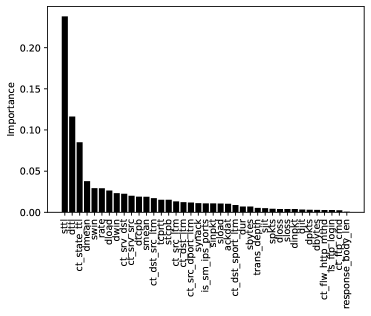
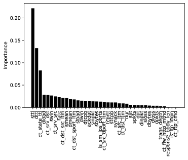
Figure 1: Risk reduction importances on UNSW-NB15. Left: PU ET. Right: PN ET.

For MNIST, the plot of the importance scores for PU ET for each digit often suggests the shape of the digit. On the other hand, the Appendix provides some additional figures that show that the normalized risk reduction importance makes many more pixels more important. This observation is consistent with our discussion in Section 4. Interestingly, the importances for PU ET appear to be very similar to those for PN ET (visually similar importance maps for MNIST, and qualitatively similar importance values which give similar feature rankings for UNSW-NB15). This suggests that the PU model is likely quite similar to the PN model.

Figure 2: Risk reduction importances learnt from ET classifier on MNIST digits. Top: PU ET with nonnegative risk estimator and quadratic loss. Bottom: PN ET with Gini impurity.

6 Related Work

PU learning was initially studied in [9, 8, 21], and many approaches have been developed based on different assumptions on the data generation mechanism.

The two-step approach discussed in the introduction have been adopted in many papers with numerous instantiations. We refer the readers to [2] for a comprehensive list.

Another important line of work, which is most related to our work and has achieved the state-of-the-art performance recently, minimizes a risk estimate based on a weighted dataset of positive and negative examples obtained by transforming the PU dataset [20, 12, 11, 16]. Our work follows the risk minimization approach, but we develop general risk minimization algorithms for learning tree models, that allows exploiting the under-explored potential of random forests.

Numerous works have been done on tree-based methods, and random forest algorithms are among the most successful ones [3, 13, 1]. In the PU learning literature, PU decision trees were explored in early works [8, 21], and PU bagging [23] has been explored for SVMs [23] and decision trees [29]. All of these approaches do not aim to directly minimize the risk.

Our recursive greedy risk minimization framework gives a new interpretation to existing tree learning algorithms for positive and negative data, and allows us to develop new algorithms for positive and unlabeled data. In addition, our approach allows us to formulate a new feature importance score that directly measures a feature’s contribution to risk minimization.

7 Conclusions

Random forests perform very well on fully supervised learning methods, but its potential in PU learning has been under-explored due to the strong emphasis on neural networks and the lack of a principled method for learning decision trees from PU data. We fill this gap in this paper. We first consider learning from positive and negative data, and develop a recursive greedy risk minimization approach for learning decision trees, and show that with suitable choice of loss functions, its instantiations are equivalent to standard impurity-based decision tree learning algorithms. We extend this approach to the PU setting, and develop a very efficient random forest algorithm which requires little hyperparameter and yet strong performance against the state-of-the-art PU learning algorithms. Our approach supports a new feature importance score that directly measures a feature’s contribution to risk mnimization.

Our work opens up some new opportunities to build tree models. First, decision trees can easily overfit the training set, and various heuristics have been used in practice to alleviate overfitting. Our recursive greedy risk minimization framework provides an alternative way to control the size of the learned decision by always expanding the node with the largest risk reduction until the risk reduction is smaller than a threshold or when the tree size is larger than a threshold. Second, we focused on quadratic loss and logistic loss in our experiments, but we can also study alternative losses such as the hinge loss, or double hinge loss.

Appendix A Proof of Theorem 1

Proof.

(a) This result is proven in [4].

(b) By grouping the positive and negative examples, we have

$$\widehat{R}_{{\rm logistic}}(v;S)=\sum_{({\bm{x}},y)\in S}w\ln(1+e^{-vy})=|S|wq_{+}\ln(1+e^{-v})+|S|wq_{-}\ln(1+e^{v}).$$

The minimizer satisfies

$$\frac{\mathrm{d}\widehat{R}_{{\rm logistic}}}{\mathrm{d}v} =|S|wq_{+}\frac{-e^{-v}}{1+e^{-v}}+|S|wq_{-}\frac{e^{v}}{1+e^{v}}=0.$$

Solving the equation, we have

$$v_{S}^{*} =\ln(q_{+}/q_{-}),$$

or $e^{v_{S}^{*}}=q_{+}/q_{-}$. Hence we have

$$\widehat{R}_{{\rm logistic}}^{*}(S)=|S|wq_{+}\ln\left(1+\frac{q_{-}}{q_{+}}\right)+|S|wq_{-}\ln\left(1+\frac{q_{+}}{q_{-}}\right)=|S|wH(S).$$

∎

Appendix B Proof of Proposition 1

Both the set $P^{\prime}\subseteq P$ and the set $U^{\prime}\subseteq U$ can possibly be empty, thus $W_{\mathsf{p}}=|P^{\prime}|w_{\mathsf{p}}\geq 0$, $W_{\mathsf{p}}+W_{{\mathsf{n}}}=|U^{\prime}|w_{\mathsf{u}}\geq 0$, and $W_{{\mathsf{n}}}=|U^{\prime}|w_{\mathsf{u}}-|P^{\prime}|w_{\mathsf{p}}$ can be negative, 0, or positive. Note that we do not consider the case that $P^{\prime}$ and $U^{\prime}$ are both empty, as this only happens when no examples are allocated to a node, which does not arise when we construct decision trees.

Proof.

(a) For the quadratic loss, we have

$$\widehat{R}_{{\rm uPU}}(v;P^{\prime},U^{\prime}) =\sum_{x\in P^{\prime}}w_{\mathsf{p}}(1-v)^{2}-\sum_{x\in P^{\prime}}w_{\mathsf{p}}(1+v)^{2}+\sum_{x\in U^{\prime}}w_{\mathsf{u}}(1+v)^{2}$$

$$=W_{\mathsf{p}}(1-v)^{2}+W_{\mathsf{n}}(1+v)^{2}.$$

If $W_{\mathsf{p}}+W_{\mathsf{n}}\neq 0$, then the partial empirical risk is a convex quadratic function with a unique minimizer satisfying

$$\frac{\text{d}\widehat{R}_{{\rm uPU}}}{\text{d}v}=-2W_{\mathsf{p}}(1-v_{P^{\prime},U^{\prime}}^{*})+2W_{\mathsf{n}}(1+v_{P^{\prime},U^{\prime}}^{*})=0.$$

Solving the equation, we have

$$v_{P^{\prime},U^{\prime}}^{*}=2v^{*}-1.$$

Therefore, we have

$$\widehat{R}_{{\rm uPU}}^{*}(P^{\prime},U^{\prime}) =(W_{\mathsf{p}}+W_{{\mathsf{n}}})v^{*}\left(1-2v^{*}+1\right)^{2}+(W_{\mathsf{p}}+W_{{\mathsf{n}}})(1-v^{*})\left(1+2v^{*}-1\right)^{2}$$

$$=4(W_{\mathsf{p}}+W_{\mathsf{n}})v^{*}\left(1-v^{*}\right).$$

If $W_{\mathsf{p}}+W_{{\mathsf{n}}}=0$, then $\widehat{R}_{{\rm uPU}}(v;P^{\prime},U^{\prime})=-2W_{\mathsf{p}}v+W_{\mathsf{p}}+2W_{\mathsf{n}}v+W_{{\mathsf{n}}}$. This gives $v_{P^{\prime},U^{\prime}}^{*}=+\infty$, and $\widehat{R}_{{\rm uPU}}^{*}(P^{\prime},U^{\prime})=-\infty$.

(b) For the logistic loss, we have

$$\widehat{R}_{{\rm uPU}}(v;P^{\prime},U^{\prime}) =\sum_{{\bm{x}}\in P^{\prime}}w_{\mathsf{p}}\ln(1+e^{-v})-\sum_{{\bm{x}}\in P^{\prime}}w_{\mathsf{p}}\ln(1+e^{v})+\sum_{{\bm{x}}\in U^{\prime}}w_{\mathsf{u}}\ln(1+e^{v})$$

$$=W_{\mathsf{p}}\ln(1+e^{-v})+W_{\mathsf{n}}\ln(1+e^{v}).$$

The derivative of the partial empirical risk wrt $v$ is

$$\frac{\text{d}\widehat{R}_{{\rm uPU}}}{\text{d}v} =\frac{W_{\mathsf{n}}e^{v}-W_{\mathsf{p}}}{1+e^{v}}.$$

By inspecting how the sign of the derivative changes as $v$ changes, we can obtain

$$v_{P^{\prime},U^{\prime}}^{*}=\begin{cases}\ln(W_{\mathsf{p}}/W_{\mathsf{n}}),&W_{\mathsf{n}}>0,W_{\mathsf{p}}>0,\\ -\infty,&W_{\mathsf{n}}>0,W_{\mathsf{p}}=0,\\ +\infty,&W_{{\mathsf{n}}}\leq 0.\end{cases}$$ (15)

with

$$\widehat{R}_{{\rm uPU}}^{*}(P^{\prime},U^{\prime})=\begin{cases}(W_{\mathsf{p}}+W_{\mathsf{n}})(-v^{*}\ln(v^{*})-(1-v^{*})\ln(1-v^{*})),&0<v^{*}<1,\\ 0,&v^{*}\in\{0,1\},\\ -\infty,&v^{*}>1.\end{cases}$$

∎

Appendix C Unbiased Estimates of Proportions

The weight $W_{\mathsf{p}}$ is an unbiased estimate of the probability $p({\bm{x}}\in\kappa,y=1)=\pi p({\bm{x}}\in\kappa\,|\,y=1)$ since $\pi|P^{\prime}|/|P|=|P^{\prime}|w_{\mathsf{p}}=W_{\mathsf{p}}$ estimates the probability $\pi p({\bm{x}}\in\kappa\,|\,y=1)$ without bias.

To show that $W_{\mathsf{n}}$ is an unbiased estimate of the probability $p({\bm{x}}\in\kappa,y=-1)$, first note that for any ${\bm{x}}$ we have $(1-\pi)p_{\mathsf{n}}({\bm{x}})=p({\bm{x}})-\pi p_{\mathsf{p}}({\bm{x}})$. Integrating over ${\bm{x}}\in\kappa$, we have $(1-\pi)p({\bm{x}}\in\kappa\,|\,y=-1)=p({\bm{x}}\in\kappa)-\pi p({\bm{x}}\in\kappa\,|\,y=1)$, or equivalently, $p({\bm{x}}\in\kappa,y=-1)=p({\bm{x}}\in\kappa)-\pi p({\bm{x}}\in\kappa\,|\,y=1)$. Now, $p({\bm{x}}\in\kappa)$ is unbiasedly estimated by $|U^{\prime}|w_{\mathsf{u}}$, and $\pi p({\bm{x}}\in\kappa\,|\,y=1)$ is unbiasedly estimated by $|P^{\prime}|w_{\mathsf{p}}$.

Appendix D Proof of Proposition 2

Proof.

To find the minimal partial nnPU empirical risk, we begin by computing the derivative of $\widehat{R}_{{\rm nnPU}}$ with respect to $v$:

$$\widehat{R}_{{\rm nnPU}}(v;P^{\prime},U^{\prime}) =\sum_{{\bm{x}}\in P^{\prime}}w_{\mathsf{p}}(1-v)^{2}+\max\left\{0,\sum_{{\bm{x}}\in U^{\prime}}w_{\mathsf{u}}(1+v)^{2}-\sum_{{\bm{x}}\in P^{\prime}}w_{\mathsf{p}}(1+v)^{2}\right\}$$

$$=W_{\mathsf{p}}(1-v)^{2}+\max\{0,W_{\mathsf{n}}(1+v)^{2}\},$$

$$\frac{\text{d}\widehat{R}_{{\rm nnPU}}}{\text{d}v} =2W_{\mathsf{p}}(v-1)+2\max\{0,W_{\mathsf{n}}\}(v+1).$$

First consider the case when $v^{*}>1$, then either $\frac{W_{\mathsf{p}}}{W_{\mathsf{p}}+W_{\mathsf{n}}}>1$ or $v^{*}=+\infty$. The former suggests that $W_{\mathsf{n}}<0$, and hence the minimizer will be 1. In the latter we have $W_{\mathsf{n}}=-W_{\mathsf{p}}\leq 0$, again giving us a minimizer of 1. On the other hand if $0\leq v^{*}<1$, then we have $W_{\mathsf{p}}\geq 0$ and $W_{\mathsf{n}}>0$ and the minimizer will be the solution to $0=\text{d}\widehat{R}_{{\rm nnPU}}/\text{d}v$.

The minimizer can thus be written succinctly as

$$\underset{v\in{\mathbb{R}}}{\mathrm{argmin}}\,\widehat{R}_{{\rm nnPU}}(v;P^{\prime},U^{\prime})=\begin{cases}1,&v^{*}>1,\\ 2v^{*}-1,&\text{otherwise},\end{cases}$$

with minimum partial empirical risk

$$\widehat{R}_{{\rm nnPU}}^{*}(v;P^{\prime},U^{\prime})=\begin{cases}0,&v^{*}>1,\\ 4(W_{\mathsf{p}}+W_{\mathsf{n}})v^{*}(1-v^{*}),&\mathrm{otherwise}.\end{cases}$$

For the logistic loss we shall again start by computing the derivative of the partial empirical risk:

$$\widehat{R}_{{\rm nnPU}}(v;P^{\prime},U^{\prime}) =W_{\mathsf{p}}\ln(1+e^{-v})+\max\{0,W_{\mathsf{n}}\ln(1+e^{v})\}$$

$$\frac{\text{d}\widehat{R}_{{\rm nnPU}}}{\text{d}v} =\frac{\max\{0,W_{\mathsf{n}}\}e^{v}-W_{\mathsf{p}}}{1+e^{v}}.$$

In this case, the minimizer $\mathrm{argmin}_{v\in{\mathbb{R}}}\widehat{R}_{{\rm nnPU}}(v;P^{\prime},U^{\prime})$ is the same as in (15). The corresponding minimum partial risk is

$$\widehat{R}_{{\rm nnPU}}^{*}(P^{\prime},U^{\prime})=\begin{cases}(W_{\mathsf{p}}+W_{\mathsf{n}})(-v^{*}\ln(v^{*})-(1-v^{*})\ln(1-v^{*})),&0<v^{*}<1,\\ 0,&\text{otherwise}.\end{cases}$$

∎

Appendix E Optimizing Split Time Complexity

Algorithm 2 gives pseudocode for finding the optimal split for a given feature. Each step is annotated with its time complexity, where $n=|P^{\prime}|+|U^{\prime}|$. Note that computing $\widehat{R}^{*}$ value can be done in constant time if $W_{\mathsf{p}}$ and $W_{{\mathsf{n}}}$ values are given. The time complexity of Algorithm 2 is $O((|P^{\prime}|+|U^{\prime}|)\ln(|P^{\prime}|+|U^{\prime}|)+m)$, with $m\leq|P^{\prime}|+|U^{\prime}|+1$.

Input: Feature $f$, set $P^{\prime}$ of positive examples and set $U^{\prime}$ of unlabeled examples.

Output: Split $(f,t)$ that gives the largest risk reduction.

1

Sort all examples ${\bm{x}}_{1},\ldots,{\bm{x}}_{n}$ in $P^{\prime}\cup U^{\prime}$ by their entries in feature $f$. Denote the sorted examples by ${\bm{x}}_{(1)},\ldots,{\bm{x}}_{(n)}$ ;

  # $O(n\ln n)$

Let the distinct $f$ values be $u_{1}<u_{2}<\ldots<u_{m+1}$, and choose $t_{i}=(u_{i}+u_{i+1})/2$, $i=1,\ldots,m$. Note $m+1\leq n$ ;

  # $O(m)$

Compute the $\widehat{R}^{*}(P^{\prime},U^{\prime})$ value by computing its $W_{\mathsf{p}}$ and $W_{{\mathsf{n}}}$ values ;

  # $O(n)$

Compute the risk reduction for $(f,t_{1})$ by computing the $W_{\mathsf{p}}$ and $W_{{\mathsf{n}}}$ values for the child nodes ;

  # $O(n)$

$t^{*}\leftarrow t_{1}$ ;

  # $O(1)$

2 for $i=2,\ldots,m$ do // $O(n)$ in total

3       Compute the risk reduction for $(f,t_{i})$. This only requires updating $W_{\mathsf{p}}$ and $W_{{\mathsf{n}}}$ values for $t_{i-1}$ by considering those ${\bm{x}}_{(i)}$ with $f$ values between $t_{i-1}$ and $t_{i}$;

4       if Risk reduction for $(f,t_{i})>$ risk reduction for $(f,t^{*})$ then

5            $t^{*}\leftarrow t_{i}$;

6       end if

7      

8 end for

Return: $t^{*}$.

Algorithm 2 Find Optimal Threshold

Appendix F Proof of Proposition 3

In addition, we show that the sigmoid loss, $\widehat{R}^{*}_{{\rm uPU}}(P^{\prime},U^{\prime})$ has an interesting interpretation.

Proof.

We have already shown that for the quadratic loss, $\widehat{R}^{*}(S)=2|S|wG(S)=4|S|wq_{+}q_{-}$.

For the savage loss, we have

$$\widehat{R}(v;S)=\sum_{(x,y)}w\frac{4}{(1+e^{vy})^{2}}=|S|w\left[q_{+}\frac{4}{(1+e^{v})^{2}}+q_{-}\frac{4}{(1+e^{-v})^{2}}\right].$$

The derivative of $\widehat{R}(v;S)$ wrt $v$ is

$$\frac{\text{d}\widehat{R}}{\text{d}v}=8|S|w\frac{-q_{+}e^{v}+q_{-}e^{2v}}{(1+e^{v})^{3}}.$$

Setting the derivative to 0, we obtain $v^{*}_{S}=\ln\frac{q_{+}}{q_{-}}$. Therefore

$$\widehat{R}^{*}(S)=|S|w\left[q_{+}\frac{4}{(1+q_{+}/q_{-})^{2}}+q_{-}\frac{4}{(1+q_{-}/q_{+})^{2}}\right]=4|S|wq_{+}q_{-},$$

which is the same as the $\widehat{R}^{*}(S)$ value for the quadratic loss. ∎

Proposition 5.

For the sigmoid loss, we have

$$\widehat{R}_{{\rm uPU}}^{*}(P^{\prime},U^{\prime})=\min\{W_{\mathsf{p}},W_{{\mathsf{n}}}\}.$$ (16)

Intuitively, the above expression uses the weight of the rarer class as the impurity measure, and we can derive a similar expression in the PN setting too. Such an impurity measure is an interesting one that has not been used in decision tree learning.

Proof.

First note that

$$\widehat{R}_{{\rm uPU}}(v;P^{\prime},U^{\prime}) =\sum_{{\bm{x}}\in P^{\prime}}\frac{w_{\mathsf{p}}}{1+e^{v}}-\sum_{{\bm{x}}\in P^{\prime}}\frac{w_{\mathsf{p}}}{1+e^{-v}}+\sum_{{\bm{x}}\in U^{\prime}}\frac{w_{\mathsf{u}}}{1+e^{-v}}$$

$$=\frac{W_{\mathsf{p}}}{1+e^{v}}+\frac{W_{\mathsf{n}}}{1+e^{-v}}$$

The derivative of the partial empirical risk is

$$\frac{\text{d}\widehat{R}_{{\rm uPU}}}{\text{d}v} =\frac{e^{v}(W_{\mathsf{n}}-W_{\mathsf{p}})}{(1+e^{v})^{2}}.$$ (17)

The equation (17) tells us that there are no stationary points in the partial empirical risk. The minimizer $v_{P^{\prime},U^{\prime}}^{*}$ is given by:

$$v_{P^{\prime},U^{\prime}}^{*}=\begin{cases}+\infty,&W_{\mathsf{p}}>W_{\mathsf{n}},\\ \text{any value},&W_{\mathsf{p}}=W_{{\mathsf{n}}},\\ -\infty,&W_{\mathsf{p}}<W_{\mathsf{n}},\\ \end{cases}=\begin{cases}+\infty,&v^{*}>0.5,\\ \text{any value},&v^{*}=0.5,\\ -\infty,&v^{*}<0.5,\\ \end{cases}$$

The corresponding minimum partial empirical risk is given by

$$\widehat{R}_{{\rm uPU}}^{*}(P^{\prime},U^{\prime})=\begin{cases}W_{\mathsf{n}},&v^{*}>0.5,\\ W_{\mathsf{p}},&v^{*}\leqslant 0.5.\end{cases}=\min\{W_{\mathsf{p}},W_{{\mathsf{n}}}\}.$$ (18)

∎

Note that we can derive similar expressions for each loss function described in Section 2, however in this paper we only focus on the quadratic and logistic loss due to their connection with the traditional Gini and entropy impurities, respectively.

Appendix G Proof of Proposition 4

Proof.

For each loss function mentioned in Section 2 we have $\ell(v,y)=a$ if $v=y$ and $\ell(v,y)=b$ if $v\neq y$, for some $0\leq a<b$ (with $a,b$ not necessarily common to all loss functions). The optimal prediction based on the uPU risk estimator is $+1$ if $\widehat{R}_{{\rm uPU}}(+1;P^{\prime},U^{\prime})<\widehat{R}_{{\rm uPU}}(-1;P^{\prime},U^{\prime})$, that is, if

$$W_{\mathsf{p}}\ell(+1,+1)+W_{\mathsf{n}}\ell(+1,-1) <W_{\mathsf{p}}\ell(-1,+1)+W_{\mathsf{n}}\ell(-1,-1)$$

$$W_{\mathsf{p}}a+W_{\mathsf{n}}b <W_{\mathsf{p}}b+W_{\mathsf{n}}a$$

$$(W_{\mathsf{p}}+W_{\mathsf{n}})/2 <W_{\mathsf{p}},$$

which happens if $v^{*}>0.5$. A symmetric argument can be applied to show that the optimal prediction is $-1$ when $v^{*}<0.5$. Continuing, observe that $a,b\geq 0$, so for the nnPU risk estimator the optimal prediction is $+1$ if

$$W_{\mathsf{p}}a+\max\{0,W_{\mathsf{n}}b\} <W_{\mathsf{p}}b+\max\{0,W_{\mathsf{n}}a\}$$

$$(b-a)\max\{0,W_{\mathsf{n}}\} <W_{\mathsf{p}}(b-a)$$

$$W_{\mathsf{n}}\leq\max\{0,W_{\mathsf{n}}\} <W_{\mathsf{p}}$$

$$W_{\mathsf{n}} <W_{\mathsf{p}},$$

which is the same result as for the uPU risk estimator. A symmetric argument shows that the optimal constant prediction based on the nnPU risk estimator is $-1$ if $v^{*}<0.5$, and hence (if we predict $-1$ when $v^{*}=0.5$ ),

$$2\mathds{1}(v^{*}>0.5)-1 =\mathrm{argmin}_{v\in\{-1,+1\}}\,\widehat{R}_{{\rm nnPU}}(v;P^{\prime},U^{\prime}).$$

We stress that this result holds for any loss function $\ell$ satisfying $\ell(v,y)>\ell(y,y)\geq 0$, with $v\neq y$. Many common loss functions satisfy this condition, including all loss functions mentioned in Section 2 as well as the hinge loss $\ell(v,y)=\max\{0,1-vy\}$, the double hinge loss $\ell(v,y)=\max\{0,(1-vy)/2,-vy\}$, the zero-one loss $\ell(v,y)=(1-\mathrm{sign}(vy))/2$, the ramp loss $\ell(v,y)=\max\{0,\min\{1,(1-vy)/2\}\}$ and the exponential loss $\ell(v,y)=\exp(-vy)$. ∎

Appendix H Pseudocode for PU ET

Our PU Extra Trees algorithm is shown in Algorithm 3, with the learning algorithm for each individual decision tree given in Algorithm 4, and the method used to find a split for a node in Algorithm 5. A nice property of this algorithm is that each tree in the forest can be trained in parallel with no need to share data between processes. Notice the similarity between Algorithm 4 and decision tree learning in the PN setting seen in Algorithm 1, with the differences being our new method for computing the prediction value at a specific node and the sub-routine for choosing a split for a node as in Algorithm 5.

To construct a random forest with 100 decision trees using the randomisation trick in Extra Trees [13], one can run PUET$(100,P,U,\lceil\sqrt{d}\rceil,1)$.

Input: $N$ - number of trees; $P$ - positive examples; $U$ - unlabeled examples; $F$ - number of attributes; $T$ - number of threshold values per attribute.

Output: Collection of trained decision trees.

1 Initialise collection of decision trees $\mathcal{T}\leftarrow\emptyset$;

2 for $i=1,\ldots,N$ do

3       Initialise the root node $\kappa_{i}$ for decision tree $i$;

4       Train a single decision tree $\mathbb{T}$ using $\texttt{Construct\_Subtree}(\kappa_{i},P,U,F,T)$;

5       $\mathcal{T}\leftarrow\mathcal{T}\cup\mathbb{T}$;

6      

7 end for

8

Return: $\mathcal{T}$

Algorithm 3 PUET$(N,P,U,F,T)$

Input: $\kappa$ - node; $P^{\prime}$ - positive examples at $\kappa$; $U^{\prime}$ - unlabeled examples at $\kappa$; $F$ -number of attributes; $T$ - number of threshold values per attribute.

Output: A (sub) decision tree $\mathbb{T}_{\kappa}$.

1 if termination criterion is met then

2       Compute optimal prediction value $v_{P^{\prime},U^{\prime}}^{*}=\mathrm{argmin}_{v\in\{-1,+1\}}\,\widehat{R}_{{\rm nnPU}}(v;P^{\prime},U^{\prime})$ for node $\kappa$;

3      

4else

5       Choose a split $(f,t)$ for node $\kappa$ using $\texttt{Find\_Split}(\kappa,F,T)$;

6       Create two child nodes $\kappa_{f>t}$ and $\kappa_{f\leq t}$ for $\kappa$ and split data into $P^{\prime}_{f>t}$, $P^{\prime}_{f\leq t}$, $U^{\prime}_{f>t}$, $U^{\prime}_{f\leq t}$;

7       $\mathbb{T}_{\kappa_{f>t}}\leftarrow$ Construct_Subtree$(\kappa_{f>t},\,P^{\prime}_{f>t},\,U^{\prime}_{f>t},F,T)$;

8       $\mathbb{T}_{\kappa_{f\leq t}}\leftarrow$ Construct_Subtree$(\kappa_{f\leq t},\,P^{\prime}_{f\leq t},U^{\prime}_{f\leq t},F,T)$;

9      

10 end if

Return: $\mathbb{T}_{\kappa}$

Algorithm 4 Construct_Subtree$(\kappa,P^{\prime},U^{\prime},F,T)$

Input: $\kappa$ - node; $F$ - number of attributes; $T$ - number of threshold values per attribute.

Output: Optimal split $(f,t)$.

1 Initialise collection of splits $\mathcal{S}\leftarrow\emptyset$;

2 Select $F$ attributes $\{f\}$ uniformly at random from all non-constant attributes at node $\kappa$;

3 for each $\{f\}$ do

4       for $i=1,\ldots,T$ do

5            Sample a random cut-point $t$ uniformly from the range of attribute $f$ at node $\kappa$;

6             $\mathcal{S}\leftarrow\mathcal{S}\cup\{(f,t)\}$;

7            

8       end for

9      

10 end for

11Choose splitting point $(f_{\kappa},t_{\kappa})\in\mathcal{S}$ that maximises the PU-data based risk reduction $\widehat{R}^{*}(P^{\prime},U^{\prime})-\widehat{R}^{*}(P^{\prime}_{f>t},U^{\prime}_{f>t})-\widehat{R}^{*}(P^{\prime}_{f\leq t},U^{\prime}_{f\leq t})$ for node $k$;

Return: $(f,t)$.

Algorithm 5 Find_Split$(\kappa,F,T)$

Appendix I Computational Efficiency of PU ET

We have run additional experiments to support our claim that PU ET is efficient. Our current Python implementation of PU ET (nnPU risk with quadratic loss) takes seconds to train a single-tree random forest on modest hardware (Intel Core i7-10700 CPU and 32 GB RAM) as shown in Table 8. Thus training a random forest is typically must faster than training a neural net.

Table 8: Training time mean (sd) in seconds for a single tree random forest.

Dataset	PU ET	PN ET (ours)	PN ET (sklearn)
20news	1.26 (0.03)	5.39 (0.09)	0.03 (0.01)
Mushroom	0.14 (0.02)	0.07 (0.01)	0.01 (0.01)
MNIST	5.90 (0.33)	37.90 (0.89)	0.34 (0.01)
CIFAR-10	16.32 (0.36)	119.78 (1.58)	0.97 (0.01)
UNSW-NB15	3.35 (0.38)	67.60 (1.48)	0.11 (0.01)

A Cython implementation of PU ET will be much faster: sklearn’s cython based implementation of PN ET (with Gini impurity) often achieves a speedup of two orders of magnitude as compared to our PN ET (with Gini impurity), on fully labeled datasets, as shown in Table 8. Note that our PN ET implementation is the same as our PU ET implementation, except different risk measures are used in the calculation of the splitting points.

Appendix J Hyperparameter Tuning for PU ET

We deliberately chose to not perform hyperparameter tuning for results in the main text to demonstrate that PU ET can be reasonably effective even without significant hyperparameter tuning. We have run some additional experiments to show that the default choice of hyperparameters offer strong performance with the benefit of decreased training times. We trained PU ET with nnPU risk estimator and quadratic loss by varying $F$ (number of sampled features) and $T$ (number of thresholds sampled for each feature) to see their effect on training time and predictive performance. Results are given in Table 9 and Table 10. All experiments here were performed on an Intel Core i7-10700 CPU with 32 GB RAM using MNIST digits, 5 replications, 100 trees in the forest and under the usual PU learning experimental setup $(|P|=1000,|U|=n)$.

Table 9: Accuracy mean% (sd) on the test set for PU ET using various hyperparameter combinations.

$F$	$T=10$	$T=1$
$d$	89.75 (0.71)	92.47 (0.54)
$\lceil\sqrt{d}\rceil$	93.24 (0.28)	93.74 (0.75)
$1$	90.02 (0.68)	81.03 (0.09)

Table 10: Training time mean (sd) in seconds for PU ET using various hyperparameter combinations.

$F$	$T=10$	$T=1$
$d$	15071.88 (172.07)	1771.92 (31.24)
$\lceil\sqrt{d}\rceil$	1231.89 (26.64)	225.65 (1.65)
$1$	370.54 (1.22)	315.42 (5.58)

The default setting $(F=\lceil\sqrt{d}\rceil,T=1)$ results in lower training times and relatively strong predictive performance. This matches the findings in the original ET paper [13] where this default was able to strike a good balance between training time and predictive performance.

Appendix K Overfitting with uPU Risk Estimators in PU ET

We performed additional experiments to empirically investigate the difference between uPU and nnPU risk estimators in regards to overfitting. In Table 11 we report the training risks (measured as PU risk as data is PU) and testing risks (measured as PN risk as data is PN) using zero-one loss $\ell_{0/1}(v,y)=(1-\mathrm{sign}(vy))/2$ on a number of datasets. Each result is reported as mean (sd) over 5 replications. From the results we can see that the training risk is significantly smaller than the test risk in the uPU setting as compared to the nnPU setting, confirming that uPU suffers more from overfitting than nnPU.

Table 11: Training and testing risk of PU ET.

Dataset		uPU		nnPU
		Quadratic	Logistic	Quadratic	Logistic
20News	Train	-0.48 (0.00)	-0.22 (0.01)	0.00 (0.00)	0.00 (0.00)
	Test	0.56 (0.00)	0.28 (0.01)	0.15 (0.00)	0.18 (0.01)
Mushroom	Train	-0.36 (0.00)	-0.01 (0.00)	0.00 (0.00)	0.00 (0.00)
	Test	0.39 (0.01)	0.01 (0.00)	0.00 (0.00)	0.00 (0.00)
MNIST	Train	-0.47 (0.00)	-0.08 (0.01)	0.00 (0.00)	0.00 (0.00)
	Test	0.49 (0.00)	0.11 (0.01)	0.04 (0.00)	0.06 (0.00)
CIFAR-10	Train	-0.38 (0.00)	-0.17 (0.01)	0.00 (0.00)	0.00 (0.00)
	Test	0.4 (0.00)	0.25 (0.00)	0.16 (0.00)	0.21 (0.00)
UNSW-NB15	Train	-0.58 (0.00)	-0.03 (0.01)	0.02 (0.01)	0.02 (0.01)
	Test	0.65 (0.00)	0.13 (0.01)	0.1 (0.01)	0.14 (0.00)

Appendix L MNIST Feature Importances

For MNIST, the plot of the importance scores for PU ET for each digit often suggests the shape of the digit. Figure 4 shows that the normalized risk reduction importance makes many more pixels more important. This observation is consistent with our discussion in Section 4. Interestingly, the importances for PU ET appear to be very similar to those for PN ET using both the risk reduction importance and normalised risk reduction importance. This suggests that the learnt PU model is likely quite similar to the learnt PN model.

Figure 3: Risk reduction importance scores for MNIST digits. Top: PU ET with nonnegative risk estimator and quadratic loss. Bottom: PN ET with quadratic loss.

Figure 4: Normalized risk (impurity) reduction importances for MNIST digits. Top: PU ET with nonnegative risk estimator and quadratic loss. Bottom: PN ET with quadratic loss.

Appendix M Feature selection with risk reduction importance

We demonstrate that the risk reduction importance is more capable of selecting features which are responsible for risk minimization and the generalization performance. We do this on the UNSW-NB15 dataset. Figure 5 shows how the accuracy of PU ET changes on UNSW-NB15 when using only top features selected by risk reduction importance and Gini impurity reduction importance. All accuracies are reported as the mean over five replications to account for randomness in sampling the P data used during training and randomness in the decision tree construction process.

With the same number of selected features, the risk reduction importance generally leads to increased accuracy on the test data compared to using Gini impurity reduction on the UNSW-NB15 dataset. The difference in area under the curve is 0.84 in favour of the risk reduction importance. This confirms that the risk reduction importance is indeed more useful for selecting features which are responsible for risk minimization and the generalization performance.

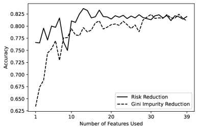
Figure 5: Risk reduction importance and Gini impurity reduction importance when using different numbers of features.

References

- [1] Susan Athey, Julie Tibshirani, and Stefan Wager. Generalized random forests. arXiv preprint: arXiv.1610.01271, 2016.
- [2] Jessa Bekker and Jesse Davis. Learning from positive and unlabeled data: A survey. Machine Learning, 109(4):719–760, 2020.
- [3] Leo Breiman. Random forests. Machine learning, 45(1):5–32, 2001.
- [4] Leo Breiman, Jerome H Friedman, Richard A Olshen, and Charles J Stone. Classification and regression trees. Routledge, 2017.
- [5] Chih-Chung Chang and Chih-Jen Lin. Libsvm: a library for support vector machines. ACM transactions on intelligent systems and technology (TIST), 2(3):1–27, 2011.
- [6] Xuxi Chen, Wuyang Chen, Tianlong Chen, Ye Yuan, Chen Gong, Kewei Chen, and Zhangyang Wang. Self-pu: Self boosted and calibrated positive-unlabeled training. In International Conference on Machine Learning, pages 1510–1519. PMLR, 2020.
- [7] Marthinus Christoffel, Gang Niu, and Masashi Sugiyama. Class-prior estimation for learning from positive and unlabeled data. In Asian Conference on Machine Learning, pages 221–236. PMLR, 2016.
- [8] Francesco De Comité, François Denis, Rémi Gilleron, and Fabien Letouzey. Positive and unlabeled examples help learning. In International conference on algorithmic learning theory, pages 219–230. Springer, 1999.
- [9] François Denis. PAC learning from positive statistical queries. In International conference on algorithmic learning theory, pages 112–126. Springer, 1998.
- [10] Marthinus Du Plessis, Gang Niu, and Masashi Sugiyama. Convex formulation for learning from positive and unlabeled data. In International conference on machine learning, pages 1386–1394. PMLR, 2015.
- [11] Marthinus C Du Plessis, Gang Niu, and Masashi Sugiyama. Analysis of learning from positive and unlabeled data. Advances in neural information processing systems, 27, 2014.
- [12] Charles Elkan and Keith Noto. Learning classifiers from only positive and unlabeled data. In Proceedings of the 14th ACM SIGKDD international conference on Knowledge discovery and data mining, pages 213–220, 2008.
- [13] Pierre Geurts, Damien Ernst, and Louis Wehenkel. Extremely randomized trees. Machine learning, 63(1):3–42, 2006.
- [14] Boris Hanin and Mark Sellke. Approximating continuous functions by relu nets of minimal width. arXiv preprint arXiv:1710.11278, 2017.
- [15] Fengxiang He, Tongliang Liu, Geoffrey I Webb, and Dacheng Tao. Instance-dependent pu learning by bayesian optimal relabeling. arXiv preprint arXiv:1808.02180, 2018.
- [16] Ryuichi Kiryo, Gang Niu, Marthinus C du Plessis, and Masashi Sugiyama. Positive-unlabeled learning with non-negative risk estimator. arXiv preprint arXiv:1703.00593, 2017.
- [17] Alex Krizhevsky, Geoffrey Hinton, et al. Learning multiple layers of features from tiny images. 2009.
- [18] Alex Krizhevsky, Geoffrey Hinton, et al. Learning multiple layers of features from tiny images. 2009.
- [19] Yann LeCun, Léon Bottou, Yoshua Bengio, and Patrick Haffner. Gradient-based learning applied to document recognition. Proceedings of the IEEE, 86(11):2278–2324, 1998.
- [20] Wee Sun Lee and Bing Liu. Learning with positive and unlabeled examples using weighted logistic regression. In ICML, volume 3, pages 448–455, 2003.
- [21] Fabien Letouzey, François Denis, and Rémi Gilleron. Learning from positive and unlabeled examples. In International Conference on Algorithmic Learning Theory, pages 71–85. Springer, 2000.
- [22] Bing Liu, Yang Dai, Xiaoli Li, Wee Sun Lee, and Philip S Yu. Building text classifiers using positive and unlabeled examples. In Third IEEE international conference on data mining, pages 179–186. IEEE, 2003.
- [23] Fantine Mordelet and J-P Vert. A bagging svm to learn from positive and unlabeled examples. Pattern Recognition Letters, 37:201–209, 2014.
- [24] Fantine Mordelet and Jean-Philippe Vert. Prodige: Prioritization of disease genes with multitask machine learning from positive and unlabeled examples. BMC bioinformatics, 12(1):1–15, 2011.
- [25] Nour Moustafa and Jill Slay. Unsw-nb15: a comprehensive data set for network intrusion detection systems (unsw-nb15 network data set). In 2015 military communications and information systems conference (MilCIS), pages 1–6. IEEE, 2015.
- [26] F. Pedregosa, G. Varoquaux, A. Gramfort, V. Michel, B. Thirion, O. Grisel, M. Blondel, P. Prettenhofer, R. Weiss, V. Dubourg, J. Vanderplas, A. Passos, D. Cournapeau, M. Brucher, M. Perrot, and E. Duchesnay. Scikit-learn: Machine learning in Python. Journal of Machine Learning Research, 12:2825–2830, 2011.
- [27] Jeffrey Pennington, Richard Socher, and Christopher D Manning. Glove: Global vectors for word representation. In Proceedings of the 2014 conference on empirical methods in natural language processing (EMNLP), pages 1532–1543, 2014.
- [28] Harish Ramaswamy, Clayton Scott, and Ambuj Tewari. Mixture proportion estimation via kernel embeddings of distributions. In International conference on machine learning, pages 2052–2060. PMLR, 2016.
- [29] Bangyu Wu, Weirong Qiu, Junxiong Jia, and Naihao Liu. Landslide susceptibility modeling using bagging-based positive-unlabeled learning. IEEE Geoscience and Remote Sensing Letters, 18(5):766–770, 2021.
- [30] Zhiang Wu, Jie Cao, Yaqiong Wang, Youquan Wang, Lu Zhang, and Junjie Wu. hpsd: a hybrid pu-learning-based spammer detection model for product reviews. IEEE transactions on cybernetics, 50(4):1595–1606, 2018.