Quantum transport in driven systems with vibrations: Floquet nonequilibrium Green’s functions and the GD approximation

Abstract

We investigate the effects of alternating voltage on nonequilibrium quantum systems with localised phonon modes. Nonequilibrium Green’s functions are utilised, with electron-phonon coupling being considered with the $GD$ approximation (self-consistent Born approximation). Using a Floquet approach, we assume periodicity of the dynamics. This approach allows us to investigate the influence of the driven electronic component on the nonequilibrium occupation of the vibrations. It was found that signatures of inelastic transport gained photon-assisted peaks. A simplistic model was proposed and found to be in good agreement with the full model in certain parameter ranges. Moreover, it was found that driving the alternating current at resonance with vibrational frequencies caused an increase in phonon occupation.

I Introduction

The transport properties of quantum dots, especially molecular junctions, can be significantly altered by vibrations coupled to the central region, causing an array of interesting phenomenacuevas2010molecular . Of particular importance is how vibrations, often in conjunction with other phenomena, inhibit device functionality and stability.

Investigations that cast vibrations as localised phonons have been extensively studied under various parameter ranges. When coupling between electronic and vibrational components is sufficiently small, differential conductance through a junction has been found to vary due to changes in bias voltage, with electrons inelastically interacting with central phononsGalperin2004a ; Galperin2004b ; cuevas2010molecular , explaining the experimental phenomena observed in inelastic electron tunnelling spectroscopy and point contact spectroscopy experimentsdjukic2005stretching ; tal2008electron ; you2017recent . For sufficiently large coupling between electrons and phonons, transport through the system is suppressed due to the Franck-Condon blockade cuevas2010molecular ; ryndyk2016theory . With semi-classical approaches to mechanical change within a junction, electron-friction and non-adiabatic effects with general potentials can be studiedpreston2020current ; Hedegard2010 ; Preston2021_first_passage ; Bode2012 ; Lu2012 ; Kershaw2020 .

In steady state, vibrations within a molecular junction have been investigated with a variety of methods Galperin2007 . Nonequilibrium Green’s functions approaches have been used to model vibrations within self-consistent perturbation theoryGalperin2004a ; Galperin2004b ; Park2011 ; Dash2010 , polaron and dressed tunnelling approximations Maier2011 ; Souto2014 , equation of motion methodsGalperin2006 and many more. Vibrations can also be studied with master equation approaches, like the Redfield master equations Peskin2020 or more involved methods like hierarchical quantum master equationsSchinabeck2020 .

Vibrations often contribute significantly to junction failure. With the current lifetime of many molecular junctions being, at best, only seconds long Darwish2020 , tackling the problem a junction instability stands as a significant hurdle for the fieldThoss2021 ; preston2020current .

The further addition of time-dependence in the form of varying voltages and electric fields is frequent within the theory and experiment surrounding molecular electronics, allowing for the probing and control of dynamics within the junction. A prime example is recent work that has seen molecular junctions probed on picosecond time-frames with a laser pulse-pair scheme Arielly2017 . Time-dependent potentials also allow for the realisation of novel functionalities, including time-dependent molecular rectifiersTu2006 ; Trasobares2016 and molecular pumpsHaughian2017 . Beyond static driving, molecular junctions are often studied within time-dependent settings, like transienceRidley2018 ; Ridley2022 , periodic driving of lead energiesHoneychurch2020 , couplingsErpenbeck2019 or by laser pulses Beltako2019 ; Ochoa2015 , when the central junction is subject to monochromatic electric fields Cabra2020 , or within the limit of slow drivings Honeychurch2019 ; Thoss2022 .

Given the importance of vibrations, understanding their dynamics under various time-dependent scenarios will be essentials for molecular junction designs that seek to capitalise on time-dependent effects. Of recent, exploration into the effects of time-dependent driving upon vibrations has been growing: transient dynamics of vibrationally active molecular junctions have been investigated theoretically with the self-consistent perturbation theory Souto2018 and dressed tunneling approximation Souto2015 ; harmonic driving of a gate voltages was used to increase current within the Franck-Condon blockade region Haughian2016 ; vibrations with perturbatively slow driving have been investigated with mean-field in a nonequilibrium Green’s functions settingHoneychurch2019 and with Hierarchical master equationsThoss2022 ; and Nonequilibrium Green’s functions and linear response theory have been utilised to investigate conductance profiles and properties of phonon under small drivingsUeda2017 ; Ueda2016 ; Ueda2011 .

Of particular interest is whether time-dependent driving can be used to reduce vibrations whilst still allowing for current flow comparable to equivalent static case. This has been predicted with a master equation approachPeskin2020 , and for vibrations modelled semi-classically with a Langevin approachPreston2020 .

Within this paper, we use a Floquet nonequilibrium Green’s function approach to investigate the effects of time-periodic driving on a single-level electronic molecule coupled to a single phonon mode, making use of the self-consistent perturbation theory in the form of the $GD$ approximationSouto2018 ; Karlsson2020 ; Ridley2022 .

It was found that changes in conductance, indicative of inelastic electron transport spectroscopy, gain photon-assisted side-peaks. Following intuition from photon-assisted transport and inelastic electron transport spectroscopy, a simplistic form for the current and phonon occupation is hypothesised and found to be a good match in limiting cases. It was also observed that resonances between the vibrational and driving frequencies resulted in increases to phonon occupation, with two different contributing mechanisms.

This paper is organized as follows: section II covers the theory. In section III, the method is applied to a single electronic level coupled with a phonon. In section IV, the results of the paper are summarized. Atomic units are used throughout the paper.

II Theory

To describe electrons moving through a junction whilst interacting with central phonons, we make use of a nonequilibrium Green’s functions approach, considering the electron-vibration coupling within the $GD$ approximation, also known as the self-consistent Born approximation.Schuler2016 ; Karlsson2020 ; Sakkinen2015

II.1 Hamiltonian

The system is modelled with the following Hamiltonian,

$$H(t)=H_{el}(t)+H_{vib}+H_{e-v}.$$ (1)

The electronic component are given by:

$$\begin{split}H_{el}(t)=H_{central}+H_{leads}(t)+H_{coupling},\end{split}$$ (2)

$$H_{central}(t)=\sum_{ij}\epsilon_{ij}d^{\dagger}_{i}d_{j},$$ (3)

$$H_{leads}(t)=\sum_{k,\alpha=L,R}\epsilon_{k\alpha}(t)c^{\dagger}_{k\alpha}c_{k\alpha},$$ (4)

$$H_{coupling}(t)=\sum_{ik\alpha=L,R}t_{k\alpha i}\;c^{\dagger}_{k\alpha}d_{i}+\mbox{h.c.}$$ (5)

and the Hamiltonian for the vibrations is given as

$$H_{vibratons}=\sum_{\alpha}\omega_{\alpha}a^{\dagger}_{\alpha}a_{\alpha},$$ (6)

and the coupling between the electronic and vibrational components is given by

$$H_{e-v}=\sum_{ij,\alpha}\lambda^{\alpha}_{i,j}Q_{\alpha}d^{\dagger}_{i}d_{j}.$$ (7)

Here, $d_{i}$ ($d^{\dagger}_{i}$) and $c_{k\alpha}$ ($c^{\dagger}_{k\alpha})$ are annihilation (creation) operators for the site $i$ in the central region and $k\alpha$ in the leads, respectively. For the phonons, the quantum operator for position is given by $Q_{\alpha}=\frac{1}{\sqrt{2}}\left(a_{\alpha}+a^{\dagger}_{\alpha}\right)$ and the momentum given by $P_{\alpha}=\frac{1}{\sqrt{2}i}\left(a_{\alpha}-a^{\dagger}_{\alpha}\right)$, where $a_{\alpha}$ $(a^{\dagger}_{\alpha})$ is the annihilation (creation) operator for the phonon $\alpha$. Within the investigation, only the energies of the leads are considered to be time-dependent. It is a simple extension to consider time-dependence within the central energy levels, $\epsilon_{ij}$ and couplings, $t_{k\alpha,i}$.

II.2 Nonequilibrium Green’s functions

To capture the dynamics of the system out of equilibrium, we make use of a nonequilibrium Green’s functions approach Schuler2016 ; Haug2008 ; Stefanucci2013 . On the Keldysh contour, we have the electronic contour Green’s function:

$$G_{ij}(\tau,\tau^{\prime})=-i\left\langle T_{c}\left(d_{i}\left(\tau\right)d^{\dagger}_{j}\left(\tau^{\prime}\right)\right)\right\rangle.$$ (8)

Similarly, we have the phononic Green’s functions,

$$\begin{split}D_{\alpha\beta}(\tau,\tau^{\prime})=-i\left\langle T_{c}\left(\Delta Q_{\alpha}\left(\tau\right)\Delta Q_{\beta}\left(\tau^{\prime}\right)\right)\right\rangle\\ =-i\left[\left\langle T_{c}\left(Q_{\alpha}\left(\tau\right)Q_{\beta}\left(\tau^{\prime}\right)\right)\right\rangle-\left\langle Q_{\alpha}\left(\tau\right)\right\rangle\left\langle Q_{\beta}\left(\tau^{\prime}\right)\right\rangle\right]\end{split}$$ (9)

and

$$\begin{split}D^{PP}_{\alpha\beta}(\tau,\tau^{\prime})=-i\left\langle T_{c}\left(\Delta P_{\alpha}\left(\tau\right)\Delta P_{\beta}\left(\tau^{\prime}\right)\right)\right\rangle\\ =-i\left[\left\langle T_{c}\left(P_{\alpha}\left(\tau\right)P_{\beta}\left(\tau^{\prime}\right)\right)\right\rangle-\left\langle P_{\alpha}\left(\tau\right)\right\rangle\left\langle P_{\beta}\left(\tau^{\prime}\right)\right\rangle\right],\end{split}$$ (10)

where $\Delta Q_{\alpha}\left(\tau\right)=Q_{\alpha}\left(\tau\right)-\left\langle Q_{\alpha}\left(\tau\right)\right\rangle$ and $\Delta P_{\alpha}\left(\tau\right)=P_{\alpha}\left(\tau\right)-\left\langle P_{\alpha}\left(\tau\right)\right\rangle$. The corresponding noninteracting Green’s functions are denoted with lower case lettering.

The current from the left or right lead is given by,

$$\begin{split}I_{\alpha}(t)=2Re\left\{\int^{\infty}_{-\infty}dt_{1}Tr\left[G^{<}(t,t_{1})\Sigma_{\alpha}^{A}(t_{1},t)\right.\right.\\ \left.\left.+G^{R}(t,t_{1})\Sigma_{\alpha}^{<}(t_{1},t)\right]\right\},\end{split}$$ (11)

and the occupation of the electrons within the central region is given by

$$n^{el}_{i}(t)=-iG_{ii}^{<}(t,t).$$ (12)

For the phonons, we are principally interested in the phonon occupation:

$$\begin{split}n^{ph}_{\alpha}(t)=\left\langle a^{\dagger}_{\alpha}\left(t\right)a_{\alpha}\left(t\right)\right\rangle\\ =\frac{1}{2}\left[\langle{P_{\alpha}(t)^{2}}\rangle+\langle{Q_{\alpha}(t)^{2}}\rangle\right]-\frac{1}{2}\\ =\frac{1}{2}\left[iD^{<}_{\alpha\alpha}\left(t,t\right)+\left\langle Q_{\alpha}(t)\right\rangle^{2}\right.\\ \left.+iD^{<,PP}_{\alpha\alpha}\left(t,t\right)+\left\langle P_{\alpha}(t)\right\rangle^{2}\right]-\frac{1}{2}.\end{split}$$ (13)

II.3 Equations of motion

To calculate the electronic and phononic nonequilibrium Green’s functions, we use the Kadanoff-Baym equations:

$$\begin{split}i\frac{\partial}{\partial\tau}G_{ij}\left(\tau,\tau^{\prime}\right)-\sum_{k}\epsilon_{ik}G_{kj}\left(\tau,\tau^{\prime}\right)\\ -\sum_{k}\int_{c}d\tau_{1}\Sigma_{ik}\left(\tau,\tau_{1}\right)G_{kj}\left(\tau_{1},\tau^{\prime}\right)=\delta_{ij}\delta_{c}\left(\tau-\tau^{\prime}\right)\end{split}$$ (14)

and

$$\begin{split}\frac{-1}{\omega_{\alpha}}\left(\frac{d^{2}}{d\tau^{2}}+\omega_{\alpha}^{2}\right)D_{\alpha\beta}\left(\tau,\tau^{\prime}\right)=\delta_{c}\left(\tau-\tau^{\prime}\right)\delta_{\alpha\beta}\\ +\sum_{\gamma}\int d\tau_{1}\Pi_{\alpha\gamma}(\tau,\tau_{1})D_{\gamma\beta}(\tau_{1},\tau^{\prime}).\end{split}$$ (15)

Here, the external influences on the central electrons and phonons is captured in $\Sigma_{ij}(\tau,\tau^{\prime})$ and $\Pi_{\alpha\beta}(\tau,\tau^{\prime})$, respectively. The collective influence on the central regions electrons can be separated into that due to the phonons and the leads:

$$\Sigma\left(\tau,\tau^{\prime}\right)=\Sigma_{int}\left(\tau,\tau^{\prime}\right)+\Sigma_{leads}\left(\tau,\tau^{\prime}\right)$$ (16)

and, similarly for the phonons,

$$\Pi\left(\tau,\tau^{\prime}\right)=\Pi_{int}\left(\tau,\tau^{\prime}\right)+\Pi_{bath}\left(\tau,\tau^{\prime}\right).$$ (17)

Calculating the electronic lead self-energies follows the standard procedure:

$$\Sigma^{<,>,R,A}_{\alpha,ij}(t,t^{\prime})=\sum_{k,k^{\prime}}t^{*}_{k\alpha,i}(t)\;g^{<,>,R,A}_{k\alpha,k^{\prime}\alpha}\left(t,t^{\prime}\right)t_{k^{\prime}\alpha,j}(t^{\prime}),$$ (18)

where the noninteracting lead self-energies follow the standard definitions,

$$g_{k\alpha,k^{\prime}\alpha^{\prime}}^{<}(t,t^{\prime})=if_{k\alpha}e^{-i\int_{t^{\prime}}^{t}dt_{1}\epsilon_{k\alpha}(t_{1})}\delta_{k,k^{\prime}},$$ (19)

$$g_{k\alpha,k^{\prime}\alpha}^{>}(t,t^{\prime})=-i(1-f_{k\alpha})e^{-i\int_{t^{\prime}}^{t}dt_{1}\epsilon_{k\alpha}(t_{1})}\delta_{k,k^{\prime}},$$ (20)

$$g^{R}_{ka,k^{\prime}a}(t,t^{\prime})=-i\Theta\left(t-t^{\prime}\right)e^{-i\int_{t^{\prime}}^{t}dt_{1}\epsilon_{k\alpha}(t_{1})}\delta_{k,k^{\prime}},$$ (21)

$$g^{A}_{ka,k^{\prime}a}(t,t^{\prime})=i\Theta\left(t^{\prime}-t\right)e^{-i\int_{t^{\prime}}^{t}dt_{1}\epsilon_{k\alpha}(t_{1})}\delta_{k,k^{\prime}}.$$ (22)

The time-dependence takes the form $\epsilon_{k\alpha}(t)=\epsilon_{k\alpha}+\phi_{\alpha}(t)$, which allows us to separate out the phase induced by the varying energies of the leads from rest of the self-energy:

$$\begin{split}\Sigma_{\alpha,ij}(t,t^{\prime})=\Sigma^{\prime}_{\alpha,ij}(t-t^{\prime})e^{-i\int_{t^{\prime}}^{t}dt_{1}\phi_{\alpha}(t_{1})}\\ =e^{-i\Phi_{\alpha}(t)}\Sigma^{\prime}_{\alpha,ij}(t-t^{\prime})e^{i\Phi_{\alpha}(t^{\prime})},\end{split}$$ (23)

where $\Phi_{\alpha}(t)$ is the anti-derivative of $\phi_{\alpha}(t)$ and $\Sigma^{\prime}_{\alpha,ij}(t-t^{\prime})$ is the self-energy of the equivalent static case, which are taken in the wide-band approximation:

$$\Sigma^{A/R}_{\alpha,ij}(\omega)=\pm\frac{i}{2}\Gamma_{\alpha,ij},$$ (24)

$$\Sigma^{<}_{\alpha,ij}(\omega)=if_{\alpha}\left(\omega\right)\Gamma_{\alpha,ij},$$ (25)

and

$$\Sigma^{>}_{\alpha,ij}(\omega)=-i\left(1-f_{\alpha}\left(\omega\right)\right)\Gamma_{\alpha,ij},$$ (26)

where the Fermi-Dirac occupation is given by:

$$f_{k\alpha}=\frac{1}{1+e^{(\epsilon_{k\alpha}-\mu_{\alpha})/T_{\alpha}}}.$$ (27)

Within the investigation, the lead energies were driven sinusoidally,

$$\phi_{\alpha}(t)=\Delta_{\alpha}\cos(\Omega_{\alpha}t),$$ (28)

which gives $\Phi(t)=\left(\Delta_{\alpha}/\Omega_{\alpha}\right)\sin\left(\Omega_{\alpha}t\right)$, which can be expressed as a Fourier series with the Jacobi-Anger expansion:

$$e^{i\frac{\Delta_{\alpha}}{\Omega_{\alpha}}\sin(\Omega_{\alpha}t)}=\sum_{n=-\infty}^{n=\infty}J_{n}\left(\frac{\Delta_{\alpha}}{\Omega_{\alpha}}\right)e^{in\Omega_{\alpha}t},$$ (29)

where $J_{n}(x)$ are Bessel functions of the first kind.

For the noninteracting phonons, we have the following phonon Green’s functions:

$$d_{\alpha\beta}^{R}(\omega)=\left[\frac{\frac{1}{2}}{\omega-\omega_{\alpha}+i\eta_{\alpha}}-\frac{\frac{1}{2}}{\omega+\omega_{\alpha}+i\eta_{\alpha}}\right]\delta_{\alpha\beta},$$ (30)

$$d_{\alpha\beta}^{A}(\omega)=\left[\frac{\frac{1}{2}}{\omega-\omega_{\alpha}-i\eta_{\alpha}}-\frac{\frac{1}{2}}{\omega+\omega_{\alpha}-i\eta_{\alpha}}\right]\delta_{\alpha\beta},$$ (31)

$$\begin{split}d_{\alpha\beta}^{<}(\omega)=-\pi i\left[f_{B}(\omega_{\alpha})\delta(\omega-\omega_{\alpha})\right.\\ \left.+(1+f_{B}(\omega_{\alpha}))\delta(\omega+\omega_{\alpha})\right]\delta_{\alpha\beta},\end{split}$$ (32)

$$\begin{split}d_{\alpha\beta}^{>}(\omega)=-\pi i\left[f_{B}(\omega_{\alpha})\delta(\omega+\omega_{\alpha})\right.\\ \left.+(1+f_{B}(\omega_{\alpha}))\delta(\omega-\omega_{\alpha})\right]\delta_{\alpha\beta}.\end{split}$$ (33)

Instead of letting $\eta_{\alpha}$ be infinitesimals, we take them as finite, so to capture the influence of a phonon bath on central phonons. Making use of fluctuation-dissipation relations, we can introduce $\eta_{\alpha}$ into the lesser and greater phonon Green’s functions:

$$\begin{split}d_{\alpha}^{<}(\omega)=\left(d_{\alpha}^{R}(\omega)-d_{\alpha}^{A}\left(\omega\right)\right)f_{B}(\omega)\\ =\left(-\frac{i\eta_{\alpha}}{\left(\omega-\omega_{\alpha}\right)^{2}+\eta_{\alpha}^{2}}+\frac{i\eta_{\alpha}}{\left(\omega+\omega_{\alpha}\right)^{2}+\eta_{\alpha}^{2}}\right)f_{B}(\omega)\end{split}$$ (34)

and

$$\begin{split}d_{\alpha}^{>}(\omega)=\left(d_{\alpha}^{R}(\omega)-d_{\alpha}^{A}\left(\omega\right)\right)\left(1+f_{B}(\omega)\right)\\ =\left(-\frac{i\eta_{\alpha}}{\left(\omega-\omega_{\alpha}\right)^{2}+\eta_{\alpha}^{2}}+\frac{i\eta_{\alpha}}{\left(\omega+\omega_{\alpha}\right)^{2}+\eta_{\alpha}^{2}}\right)\left(1+f_{B}(\omega)\right),\end{split}$$ (35)

where taking the limit of $\eta$,

$$\lim_{\eta\rightarrow 0^{+}}\left[\frac{\eta}{\left(\omega-\omega_{0}\right)^{2}+\eta^{2}}\right]\rightarrow\pi\delta\left(\omega-\omega_{0}\right),$$ (36)

and substituting for $f^{0}_{B}(-\omega)=-\left(f^{0}_{B}(\omega)+1\right)$, gives us back the equations (32) and (33).

For the lesser and greater phonon Green’s functions, we can use the fluctuation-dissipation rules to cast the effects due to the infinitesimals as self-energies. Equating equations (32) and (33) with the associated Keldysh equations gives us:

$$\Pi_{\alpha}^{</>}\left(\omega\right)=\mp 4i\eta_{\alpha}\left(\frac{\omega}{\omega_{\alpha}}\right)f_{B}(\pm\omega).$$ (37)

This phonon self-energy is used to incorporate the effects of the infinitesimal into self-consistent calculations (see equation (17)).

In addition to the above Green’s functions, we need to calculate $\left\langle Q_{\alpha}(\tau)\right\rangle$, $\left\langle P_{\alpha}(\tau)\right\rangle$ and $D^{PP}_{\alpha,\alpha^{\prime}}\left(\tau,\tau^{\prime}\right)$, allowing for the calculation of the phonon occupation. The equation of motion for the average position is given as Schuler2016 ,

$$\begin{split}\frac{-1}{\omega_{\alpha}}\left(\frac{d^{2}}{d\tau^{2}}+\omega_{\alpha}^{2}\right)\left\langle Q_{\alpha}(\tau)\right\rangle=\sum_{ij}-i\lambda^{\alpha}_{ij}G_{ji}\left(\tau,\tau^{+}\right)\\ +\int d\tau_{1}\Pi^{bath}_{\alpha}(\tau,\tau_{1})\left\langle Q_{\alpha}(\tau_{1})\right\rangle.\end{split}$$ (38)

For the terms with momentum operators, we make use of

$$\frac{d}{d\tau}Q_{\alpha}(\tau)=\omega_{\alpha}P_{\alpha}(\tau),$$ (39)

which gives us the equations of motions

$$\frac{d}{d\tau}\langle{Q_{\alpha}(\tau)}\rangle=\omega_{\alpha}\langle{P_{\alpha}(\tau)}\rangle$$ (40)

and

$$\begin{split}\frac{d}{d\tau d\tau^{\prime}}D_{\alpha\beta}\left(\tau,\tau^{\prime}\right)=\omega_{\alpha}\delta_{\alpha\beta}\delta\left(\tau,\tau^{\prime}\right)\\ +D^{PP}_{\alpha\beta}\left(\tau,\tau^{\prime}\right)\omega_{\alpha}\omega_{\beta}.\end{split}$$ (41)

These objects allows us to calculate occupation:

$$\begin{split}n^{ph}_{\alpha}(\tau)=\left\langle T_{c}\left(a_{\alpha}\left(\tau\right)a_{\alpha}^{\dagger}\left(\tau^{+}\right)\right)\right\rangle\\ =\frac{1}{2}\left[\left\langle T_{c}\left(Q^{2}_{\alpha}\left(\tau\right)\right)\right\rangle+\left\langle T_{c}\left(P^{2}_{\alpha}\left(\tau\right)\right)\right\rangle\right]-\frac{1}{2}\\ =\frac{1}{2}\left[iD_{\alpha\alpha}\left(\tau,\tau^{+}\right)+\left\langle Q_{\alpha}(\tau)\right\rangle^{2}\right.\\ \left.+iD^{PP}_{\alpha\alpha}\left(\tau,\tau^{+}\right)+\left\langle P_{\alpha}(\tau)\right\rangle^{2}\right]-\frac{1}{2}.\end{split}$$ (42)

The interaction between electrons and phonons can be approximated within the GD approximation Sakkinen2015 ; Karlsson2020 :

$$\mathbf{\Sigma}_{ij}^{int}(\tau,\tau^{\prime})=\mathbf{\Sigma}_{ij}^{har}(\tau,\tau^{\prime})+\mathbf{\Sigma}_{ij}^{XC}(\tau,\tau^{\prime}),$$ (43)

where

$$\begin{split}\mathbf{\Sigma}_{ij}^{har}(\tau,\tau^{\prime})\\ =-i\delta\left(\tau,\tau^{\prime}\right)\sum_{\beta}\lambda^{\beta}_{ij}\int_{c}d\tau_{1}d_{\beta}(\tau,\tau_{1})\sum_{ml}\lambda_{ml}^{\beta}G_{lm}(\tau_{1},\tau_{1}^{+}),\end{split}$$ (44)

$$\mathbf{\Sigma}^{XC}_{ij}(\tau,\tau^{\prime})=i\sum_{\mu\nu,ml}D_{\mu\nu}\left(\tau,\tau^{\prime}\right)\lambda^{\mu}_{im}G_{ml}\left(\tau,\tau^{\prime}\right)\lambda^{\nu}_{lj},$$ (45)

and

$$\Pi^{int}_{\alpha\beta}(\tau,\tau^{\prime})=-i\sum_{mlkp}\lambda^{\alpha}_{ml}G_{lk}\left(\tau,\tau^{\prime}\right)\lambda^{\beta}_{kp}G_{pm}\left(\tau^{\prime},\tau\right).$$ (46)

II.4 Floquet Theory

Moving the equations of motion from the contour to real time with the greater, lesser, retarded and advanced projections Haug2008 ; Rammer2007 , we can solve the equations of motion with a Floquet approach Honeychurch2020 ; Brandes1997 , where we assume that the system is time-periodic around the central time $T=\frac{t+t^{\prime}}{2}$, and complete a Fourier transform with respect to the relative time, $\tau=t-t^{\prime}$:

$$A(t,t^{\prime})=A(T,\tau)=\sum^{\infty}_{n=-\infty}A(\tau,n)e^{\Omega inT}$$ (47)

and

$$A\left(\omega,n\right)=\frac{1}{P}\int^{P}_{0}dT\;e^{-i\Omega nT}\int^{\infty}_{-\infty}d\tau e^{i\omega\tau}A(T,\tau).$$ (48)

For solving the convolutions of the form

$$C(t,t^{\prime})=\int dt_{1}A(t,t_{1})B(t_{1},t^{\prime}),$$ (49)

we recast the Fourier coefficients into a Floquet matrix,

$$\bar{A}\left(\omega,m,n\right)=A\left(\omega+\frac{\Omega}{2}\left(m+n\right),n-m\right),$$ (50)

which allows us to express the convolution as a matrix multiplication,

$$\bar{C}\left(\omega,m,n\right)=\sum_{r=-\infty}^{\infty}\bar{A}\left(\omega,m,r\right)\bar{B}\left(\omega,r,n\right),$$ (51)

allowing for the Kadanoff-Baym equations to be written as a matrix equation:

$$\begin{split}\left(\omega+\Omega m\right)\bar{G}_{ij}^{R/A}\left(\omega,m,n\right)-\sum_{k}\epsilon_{ik}\bar{G}_{kj}^{R/A}\left(\omega,m,n\right)=\\ \delta_{ij}\delta_{mn}+\sum_{k,r}\bar{\Sigma}_{ik}^{R/A}\left(\omega,m,r\right)\bar{G}_{kj}^{R/A}\left(\omega,r,n\right),\end{split}$$ (52)

$$\begin{split}\bar{G}_{ij}^{<}(\omega,m,n)=\\ \sum_{kw,rs}\bar{G}_{ik}^{R}(\omega,m,r)\bar{\Sigma}^{<}_{kw}\left(\omega,r,s\right)\bar{G}_{wj}^{A}\left(\omega,s,n\right),\end{split}$$ (53)

$$\begin{split}\frac{-1}{\omega_{\alpha}}\left(\omega^{2}_{\alpha}-\left(\omega+\Omega m\right)^{2}\right)\bar{D}^{R}_{\alpha\beta}\left(\omega,m,n\right)=\delta_{\alpha\beta}\delta_{mn}\\ +\sum_{\gamma,r}\bar{\Pi}_{\alpha\gamma}\left(\omega,m,r\right)\bar{D}_{\gamma\beta}\left(\omega,r,n\right),\end{split}$$ (54)

$$\begin{split}\bar{D}_{\alpha\beta}^{<}(\omega,m,n)\\ =\sum_{\nu\gamma,rs}\bar{D}_{\alpha\nu}^{R}(\omega,m,r)\bar{\Pi}^{<}_{\nu\gamma}\left(\omega,r,s\right)\bar{D}_{\gamma\beta}^{A}\left(\omega,s,n\right).\end{split}$$ (55)

Other important objects transform in a similar manner. The lead self-energies, equation (23), making use of equations (29) and (51), transform to

$$\bar{\Sigma}_{\alpha,ij}\left(\omega,m,n\right)=\sum_{pq,lk}\bar{S}_{\alpha}\left(m,p\right){\bar{\Sigma}^{\prime}}_{\alpha,lk}\left(\omega,p,q\right){\bar{S}}_{\alpha}\left(n,q\right),$$ (56)

where $\bar{S}_{\alpha}\left(m,n\right)=J_{m-n}\left(\Delta_{\alpha}/\Omega_{\alpha}\right)$. The Fourier coefficients of the current and occupation can be taken from the Floquet matrices derived from equations (11) and (12):

$$\begin{split}I_{\alpha}(n-m)=\bar{I}_{\alpha}\left(m,n\right)\\ =2\int^{\infty}_{-\infty}\frac{d\omega}{2\pi}\sum_{r,ij}\left[\bar{G}_{ij}^{R}(\omega,m,r)\bar{\Sigma}^{<}_{ji}\left(\omega,r,n\right)\right.\\ \left.+\bar{G}_{ij}^{<}(\omega,m,r)\bar{\Sigma}^{R}_{ji}\left(\omega,r,n\right)\right]\end{split}$$ (57)

and

$$\begin{split}n_{j}^{el}\left(n-m\right)=\bar{n}_{j}^{el}\left(m,n\right)=-i\int^{\infty}_{-\infty}\frac{d\omega}{2\pi}\bar{G}_{jj}^{<}(\omega,m,n),\end{split}$$ (58)

The time-resolved observables can then be found with equation (47), where $t\rightarrow t^{\prime}$, and by taking only the real part, as per equations (12) and (11).

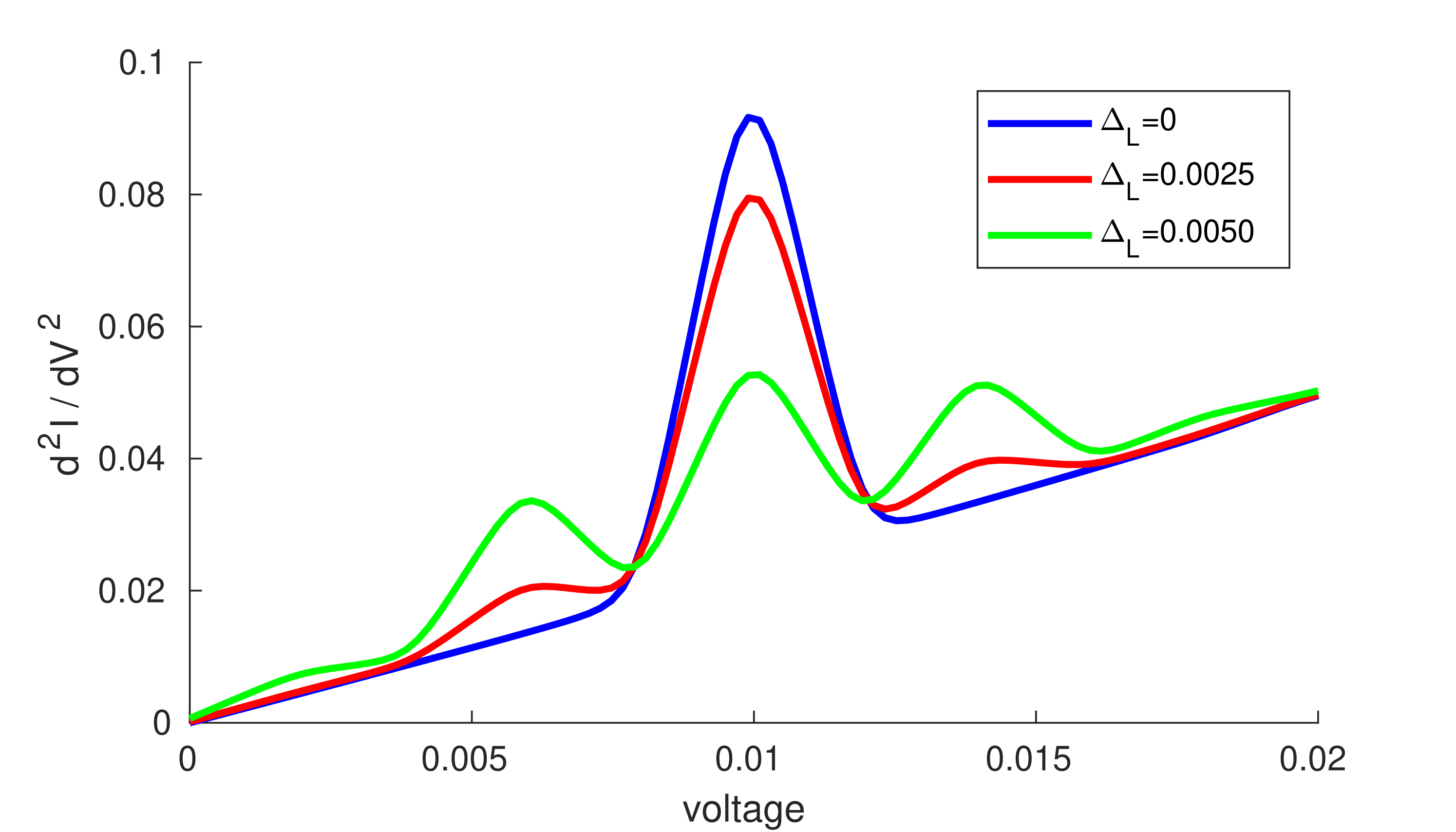
(a)

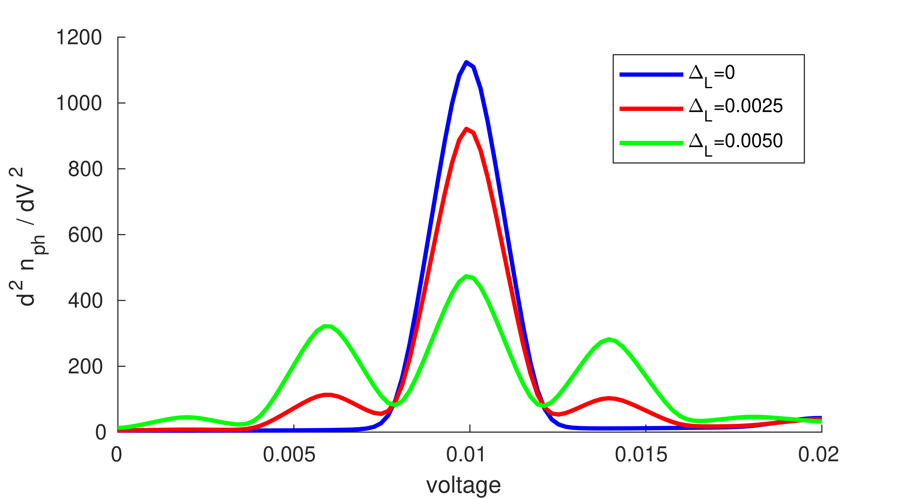
(b)

Figure 1: The changes in $d^{2}I/dV^{2}$ and $d^{2}n_{ph}/dV^{2}$ as voltage increases, given different driving energies $\Delta_{L}$. The other parameters are $\Gamma_{L}=\Gamma_{R}=0.015$, $\epsilon_{c}=0.1$, $\eta_{c}=3\times 10^{-5}$, $\Omega=0.004$, $\omega_{c}=0.01$, $\lambda_{c}=0.015$ and $T=1.5\times 10^{-4}$. The bounds of the integrand were taken at $-0.3$ and $0.3$. Fourier coefficients ranging from -8 to 8 were used in the calculation. The uniform grid spacing was $2\times 10^{-5}$. The convergence was below $10^{-6}$ for both the electronic and phonon occupation.

Unfortunately, the interaction self-energies cannot be brought to such an amenable form, and must be calculated from the Fourier coefficients. The interaction self-energies follow the forms

$$C_{XC}(t,t^{\prime})=A\left(t,t^{\prime}\right)B\left(t,t^{\prime}\right),$$ (59)

$$C_{POL}(t,t^{\prime})=A\left(t,t^{\prime}\right)B\left(t^{\prime},t\right),$$ (60)

$$C_{HAR}(t,t^{\prime})=\delta\left(t-t^{\prime}\right)\int^{\infty}_{-\infty}dt_{1}A(t,t_{1})B(t_{1},t_{1}).$$ (61)

Applying the Floquet tranformation to the above gives

$$\begin{split}C_{XC}\left(\omega,n\right)\\ =\sum_{m=-\infty}^{\infty}\int\frac{d\omega^{\prime}}{2\pi}A(\omega^{\prime},m)B(\omega-\omega^{\prime},n-m),\end{split}$$ (62)

$$\begin{split}C_{POL}\left(\omega,n\right)\\ =\sum_{m=-\infty}^{\infty}\int\frac{d\omega^{\prime}}{2\pi}A(\omega^{\prime},m)B(\omega^{\prime}-\omega,n-m)\end{split}$$ (63)

and

$$\begin{split}C_{HAR}(\omega,n)\\ =\sum^{\infty}_{m=-\infty}A\left(-\frac{\Omega}{2}\left(n+m\right),n-m\right)B^{\prime}\left(n\right).\end{split}$$ (64)

The $C_{HAR}\left(\omega,n\right)$ simplifies when $A(t,t^{\prime})=A(t-t^{\prime})$, giving us

$$\begin{split}C_{HAR}\left(\omega,n\right)\\ =\sum^{\infty}_{m=-\infty}\delta_{m,n}A(-\frac{\Omega}{2}\left(m+n\right),0)B(n)\\ =A(-\Omega n,0)B(n).\end{split}$$ (65)

The above allow us to cast the interaction self-energies in terms of their Fourier coefficients:

$$\begin{split}\Sigma^{R}_{har,ij}\left(\omega,r\right)=\\ -i\sum_{\beta}\lambda^{\beta}_{ij}d^{R}_{\beta}(\omega=-\Omega r)\int\frac{d\omega}{2\pi}\sum_{kw}\lambda_{kw}^{\beta}G_{wk}^{<}(\omega,r)\end{split}$$ (66)

$$\begin{split}\Sigma^{R}_{XC,ij}\left(\omega,r\right)=\int\frac{d\omega^{\prime}}{2\pi}\sum^{\infty}_{n=-\infty}\sum_{\mu\nu,ml}\\ iD^{<}_{\mu\nu}\left(\omega^{\prime},n\right)\lambda^{\mu}_{im}G^{R}_{ml}\left(\omega-\omega^{\prime},r-n\right)\lambda^{\nu}_{lj}\\ +iD^{R}_{\mu\nu}\left(\omega^{\prime},n\right)\lambda^{\mu}_{im}G^{<}_{ml}\left(\omega-\omega^{\prime},r-n\right)\lambda^{\nu}_{lj}\\ +iD^{R}_{\mu\nu}\left(\omega^{\prime},n\right)\lambda^{\mu}_{im}G^{R}_{ml}\left(\omega-\omega^{\prime},r-n\right)\lambda^{\nu}_{lj}\end{split}$$ (67)

$$\begin{split}\Sigma^{<}_{XC,ij}\left(\omega,r\right)=\int\frac{d\omega^{\prime}}{2\pi}\sum^{\infty}_{n=-\infty}\sum_{\mu\nu,ml}\\ iD^{<}_{\mu\nu}\left(\omega^{\prime},n\right)\lambda^{\mu}_{im}G^{<}_{ml}\left(\omega-\omega^{\prime},r-n\right)\lambda^{\nu}_{lj}\end{split}$$ (68)

$$\begin{split}\Sigma^{>}_{XC,ij}\left(\omega,r\right)=\int\frac{d\omega^{\prime}}{2\pi}\sum^{\infty}_{n=-\infty}\sum_{\mu\nu,ml}\\ iD^{>}_{\mu\nu}\left(\omega^{\prime},n\right)\lambda^{\mu}_{im}G^{>}_{ml}\left(\omega-\omega^{\prime},r-n\right)\lambda^{\nu}_{lj}\end{split}$$ (69)

$$\begin{split}\Pi^{R}_{\alpha\beta}(\omega,r)=\int\frac{d\omega^{\prime}}{2\pi}\sum^{\infty}_{n=-\infty}\sum_{mlkp}\\ -i\lambda^{\alpha}_{ml}G^{<}_{lk}\left(\omega^{\prime},n\right)\lambda^{\beta}_{kp}G^{A}_{pm}\left(\omega^{\prime}-\omega,r-n\right)\\ -i\lambda^{\alpha}_{ml}G^{R}_{lk}\left(\omega^{\prime},n\right)\lambda^{\beta}_{kp}G^{<}_{pm}\left(\omega^{\prime}-\omega,r-n\right)\end{split}$$ (70)

$$\begin{split}\Pi_{\alpha\beta}^{<}(\omega,r)=\int\frac{d\omega^{\prime}}{2\pi}\sum^{\infty}_{n=-\infty}\sum_{mlkp}\\ -i\lambda^{\alpha}_{ml}G^{<}_{lk}\left(\omega^{\prime},n\right)\lambda^{\beta}_{kp}G^{>}_{pm}\left(\omega^{\prime}-\omega,r-n\right)\end{split}$$ (71)

$$\begin{split}\Pi_{\alpha\beta}^{>}(\omega,r)=\int\frac{d\omega^{\prime}}{2\pi}\sum^{\infty}_{n=-\infty}\sum_{mlkp}\\ -i\lambda^{\alpha}_{ml}G^{>}_{lk}\left(\omega^{\prime},n\right)\lambda^{\beta}_{kp}G^{<}_{pm}\left(\omega^{\prime}-\omega,r-n\right).\end{split}$$ (72)

Solving equation (38), we can cast the average phonon positions, and the subsequent average phonon momenta, in terms of Fourier coefficients

$$\begin{split}\left\langle Q_{\alpha}\right\rangle(r)\\ =-id^{R}_{\alpha}\left(\omega=-\Omega r\right)\int\frac{d\omega}{2\pi}\sum_{ml}\lambda_{ml}^{\alpha}G_{lm}^{<}\left(\omega,r\right),\end{split}$$ (73)

$$\left\langle P_{\alpha}\right\rangle(r)=\frac{ir\Omega}{\omega_{0}}\left\langle Q_{\alpha}\right\rangle(r).$$ (74)

We can complete a similar process for the phonon momentum Green’s functions, allowing us to calculate variance of the momentum operators:

$$\begin{split}\left\langle\left(\Delta P_{\alpha}\right)^{2}\right\rangle(r)=iD_{\alpha\alpha}^{PP,<}(r)\\ =\frac{i}{{\omega_{0}}^{2}}\int\frac{d\omega}{2\pi}\left(\omega^{2}-\left(\frac{r\Omega}{2}\right)^{2}\right)D_{\alpha\alpha}^{<}(\omega,r).\end{split}$$ (75)

II.5 Implementation

Solving for the Green’s functions, the dimensions of the Floquet matrices, and the corresponding Fourier series, need to be truncated. The addition of more Fourier coefficients leads more accurate results, converging on the exact result. Calculating the integrand of the Fourier coefficients was completed with equidistant grid of points. Completing this procedure for the noninteracting case, the Floquet matrices were unravelled to Fourier coefficients using equation (50). The terms where $n+m=0,-1$ of $\bar{A}\left(\omega,m,n\right)$, where taken for calculating the Fourier coefficients. These were then used to calculate the interaction self-energies before being reassembled into the Floquet matrices. The process was then completed iteratively, with convergence given by the Fourier coefficients of the phonon and electron occupations:

$$\begin{split}\frac{\sum_{m}\left|n_{m}^{k+1}-n_{m}^{k}\right|}{\sum_{m}\left|n^{k}_{m}\right|}\leq\delta,\end{split}$$ (76)

where $n^{k}_{m}$ is the $k$th iteration of the $m$th Fourier coefficent of the occupation in question, with $\delta$ as the convergence.

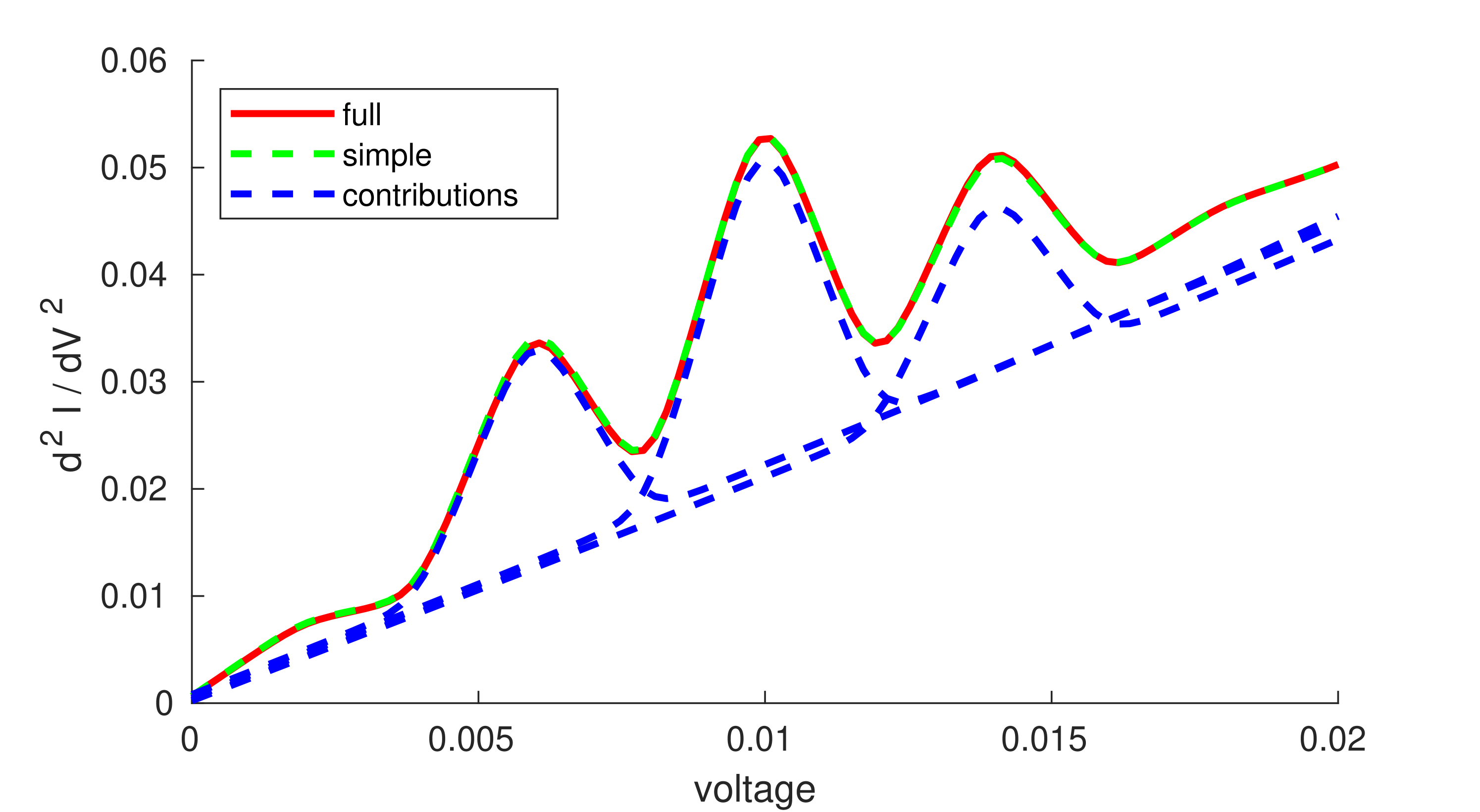
(a)

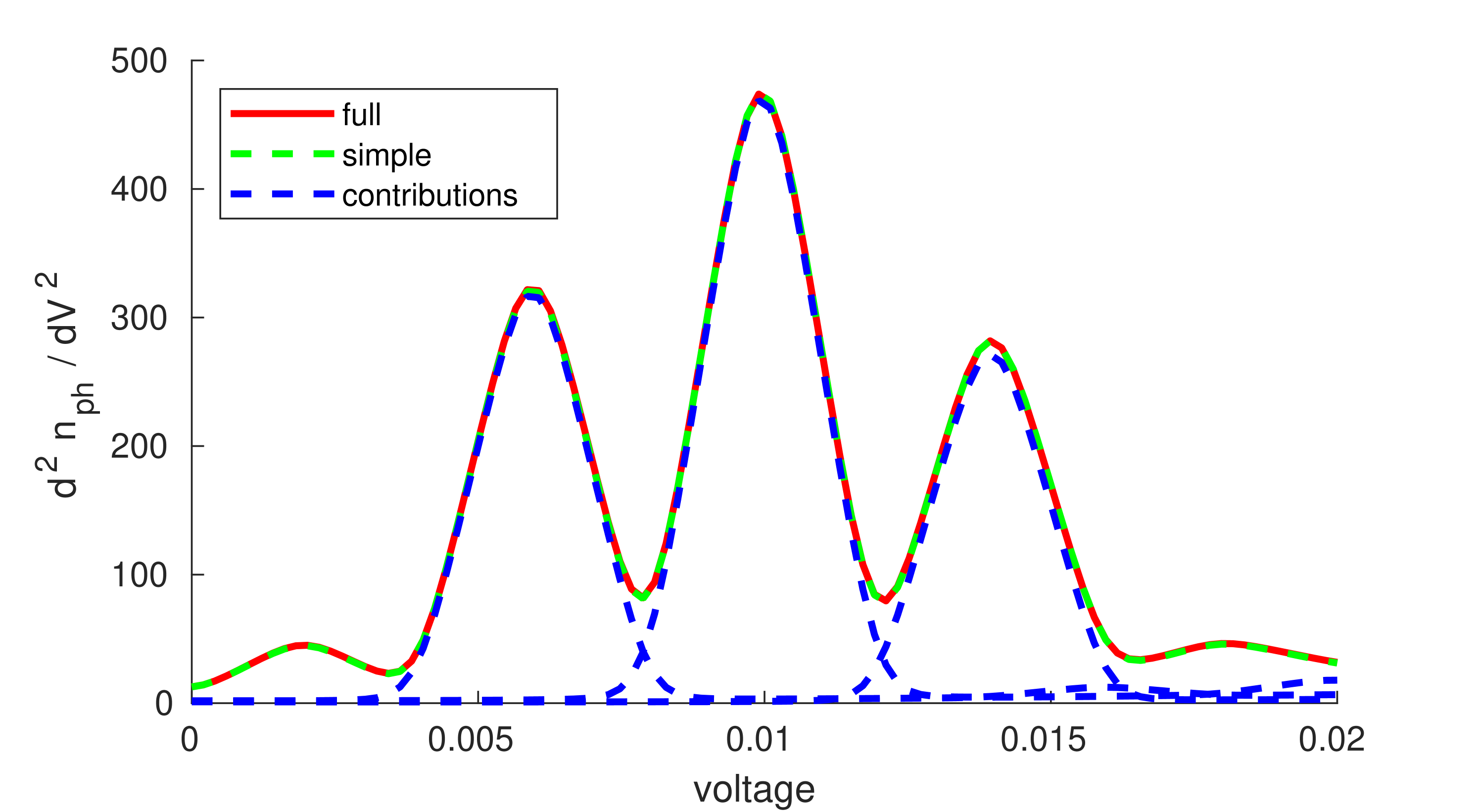
(b)

Figure 2: The changes in $d^{2}I/dV^{2}$ and $d^{2}n_{ph}/dV^{2}$ as voltage increases. Here, the full method is plotted alongside the simplistic method and contributions from $n=-1,0,1$ of equation (78). The other parameters are $\Gamma_{L}=\Gamma_{R}=0.015$, $\epsilon_{c}=0.1$, $\eta_{c}=3\times 10^{-5}$, $\Omega=0.004$, $\omega_{c}=0.01$, $\lambda_{c}=0.015$, $\Delta_{L}=0.005$ and $T=1.5\times 10^{-4}$. The bounds of the integrands were taken at $-0.3$ and $0.3$. Fourier coefficients ranging from -8 to 8 were used in the calculation. The uniform grid spacing was $2\times 10^{-5}$. The convergence was below $10^{-6}$ for both the electronic and phonon occupations.

III Results

For simplicity, we focus on a single electronic level coupled to a single phonon mode, with driving within the left lead:

$$\begin{split}H\left(t\right)=\epsilon_{c}d^{\dagger}d+\sum_{ik\alpha=L,R}t_{k\alpha i}\;c^{\dagger}_{k\alpha}d+t^{*}_{k\alpha i}\;d^{\dagger}c_{k\alpha}\\ +\sum_{k}\left(\epsilon_{kL}+\Delta_{L}\cos(\Omega t)\right)c^{\dagger}_{kL}c_{kL}+\epsilon_{kR}c^{\dagger}_{kR}c_{kR}\\ +\;\omega_{c}a^{\dagger}a+\lambda_{c}Qd^{\dagger}d.\end{split}$$ (77)

The parameters for the model consist of $\epsilon_{c}$, the energy of the central level, $\omega_{c}$, the vibrational frequency of the phonon mode, $\Omega$, the driving frequency of the left lead, $\Delta_{L}$ the magnitude of the driving in the left lead, $\Gamma_{L/R}$, the couplings to the leads, $\lambda_{c}$, the coupling strength between the central level and phonon, $\eta_{c}$, the coupling of the phonon to its bath and the temperature of both leads, $T$. Within the calculations, the driving frequency of the left lead is used as the frequency for the system’s periodicity.

For the time-averaged picture of this model, we have two important limiting cases in the static, interacting case and the noninteracting case. The static case is well understood and extensively studiedGalperin2004a ; Galperin2004b ; Galperin2007 ; cuevas2010molecular . In this context, the phonon mode causes elastic corrections and facilitates new, inelastic channels of transport through the junction, by means of absorption or emission of phonons. The latter only occurs when the voltage window widens to accommodate electrons that enter the junction before absorbing (emitting) a phonon of energy. The addition of extra channels through junction can be seen in subtle changes to the current, captured as peaks in the derivative of the differential conductance with respect to voltage.

The noninteracting case has also been extensively studied, and can be explained with the notion of photon-assisted transport Jauho1994 ; Haug2008 ; Platero2004 . The periodic driving of the system (environment) results in contributions to the time-averaged observables from the equivalent static cases, with the driven energies shifted by integer multiples of the driving frequency of the time-dependence. This can be interpreted as a proportion of the electrons emitting or absorbing quanta of the energy, hence the name photon-assisted transport. For the driving used in this paper, see equation (28), limited to the left lead, we have

$$\begin{split}\frac{1}{P}\int^{P}_{0}I_{\alpha}(t)dt=\\ \sum^{n=\infty}_{n=-\infty}\left(J_{n}\left(\frac{\Delta_{\alpha}}{\Omega_{\alpha}}\right)\right)^{2}\;I^{DC}_{\alpha}\left(\mu_{L}+n\Omega,\mu_{R}\right),\end{split}$$ (78)

Where, $I_{\alpha}(t)$ is the AC-driven current through lead $\alpha$ and $I^{DC}_{a}$ is the static case, where no driving is present.

Within certain parameter regimes, combining the reasoning from both limiting cases explains the features observed in the full model. In figure (1(a)), we see the primary peak within $dI^{2}/dV^{2}$, indicative of inelastic collisions, gain additional satellite peaks due to absorption (emission) of quanta of energy by the electrons, prior to entering the junction, per photon-assisted tunnelling. A similar effect is observed within figure (1(b)), with $d^{2}n_{ph}/dV^{2}$ gaining photon-assisted sidepeaks, suggesting that the photon-assisted side-peaks of left lead contribute to the occupation of the phonon independently of each other.

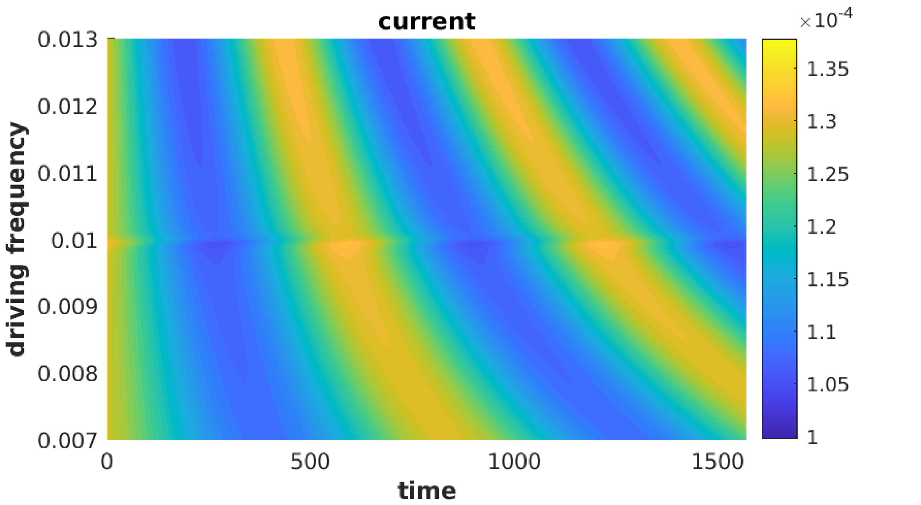
(a)

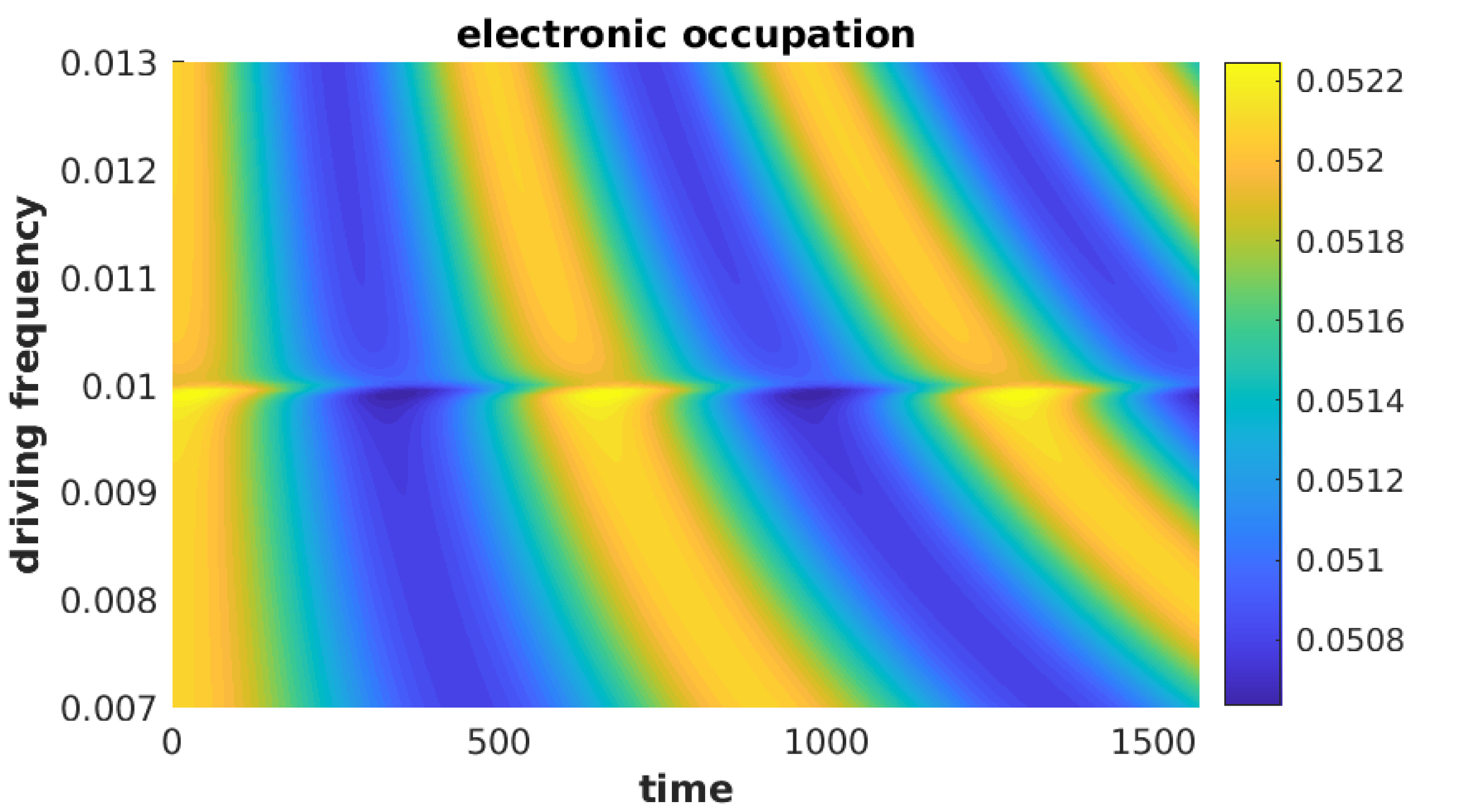
(b)

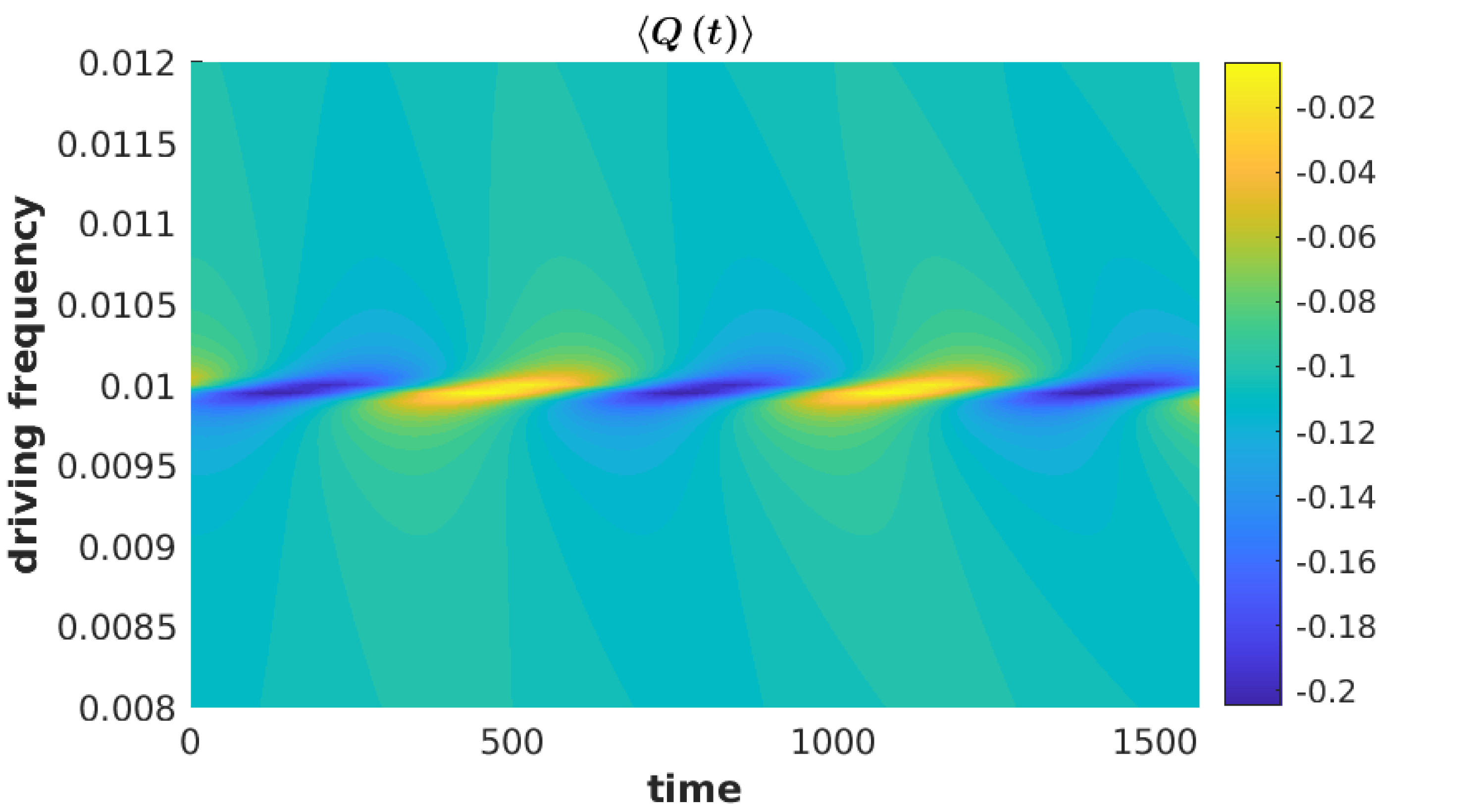
(c)

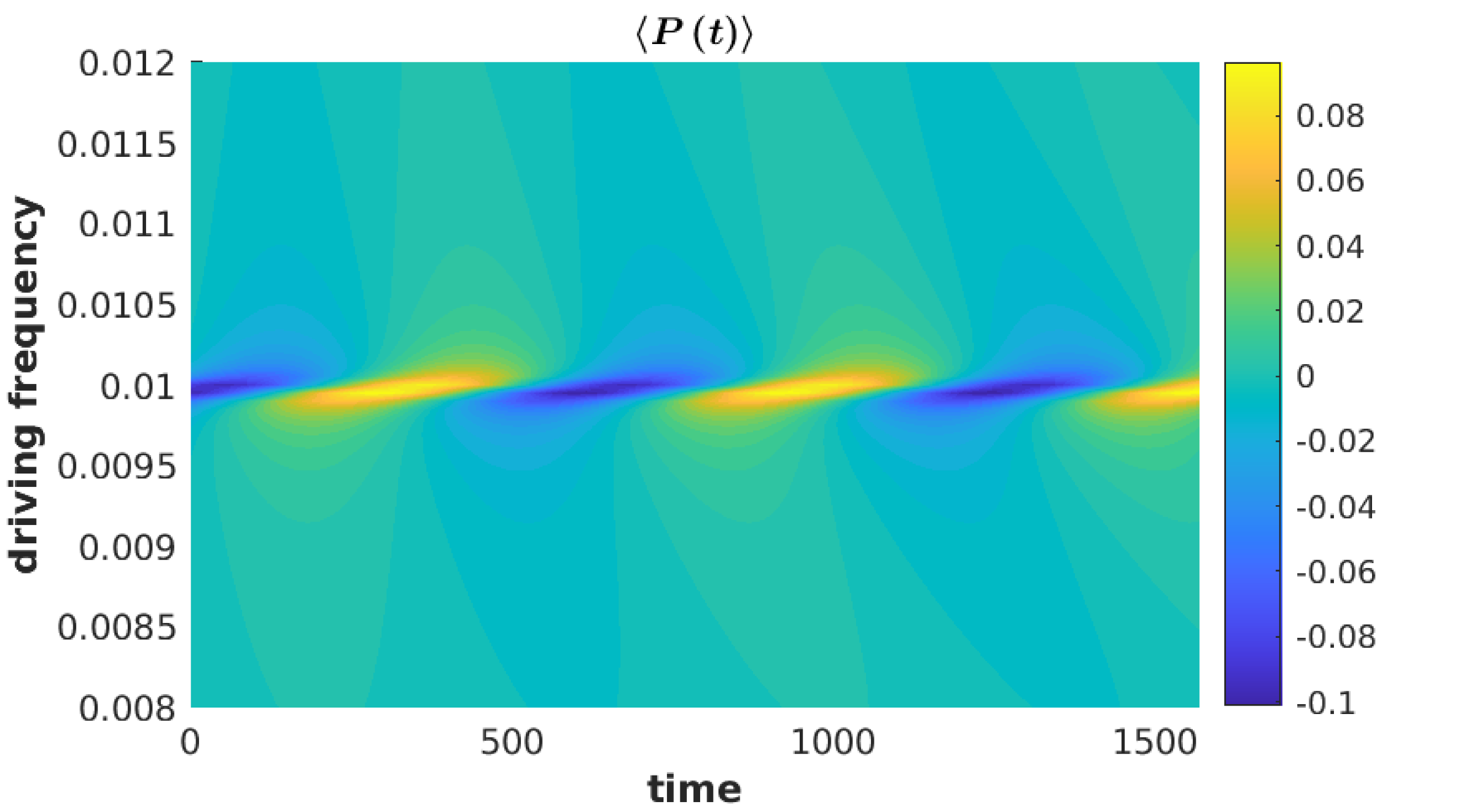
(d)

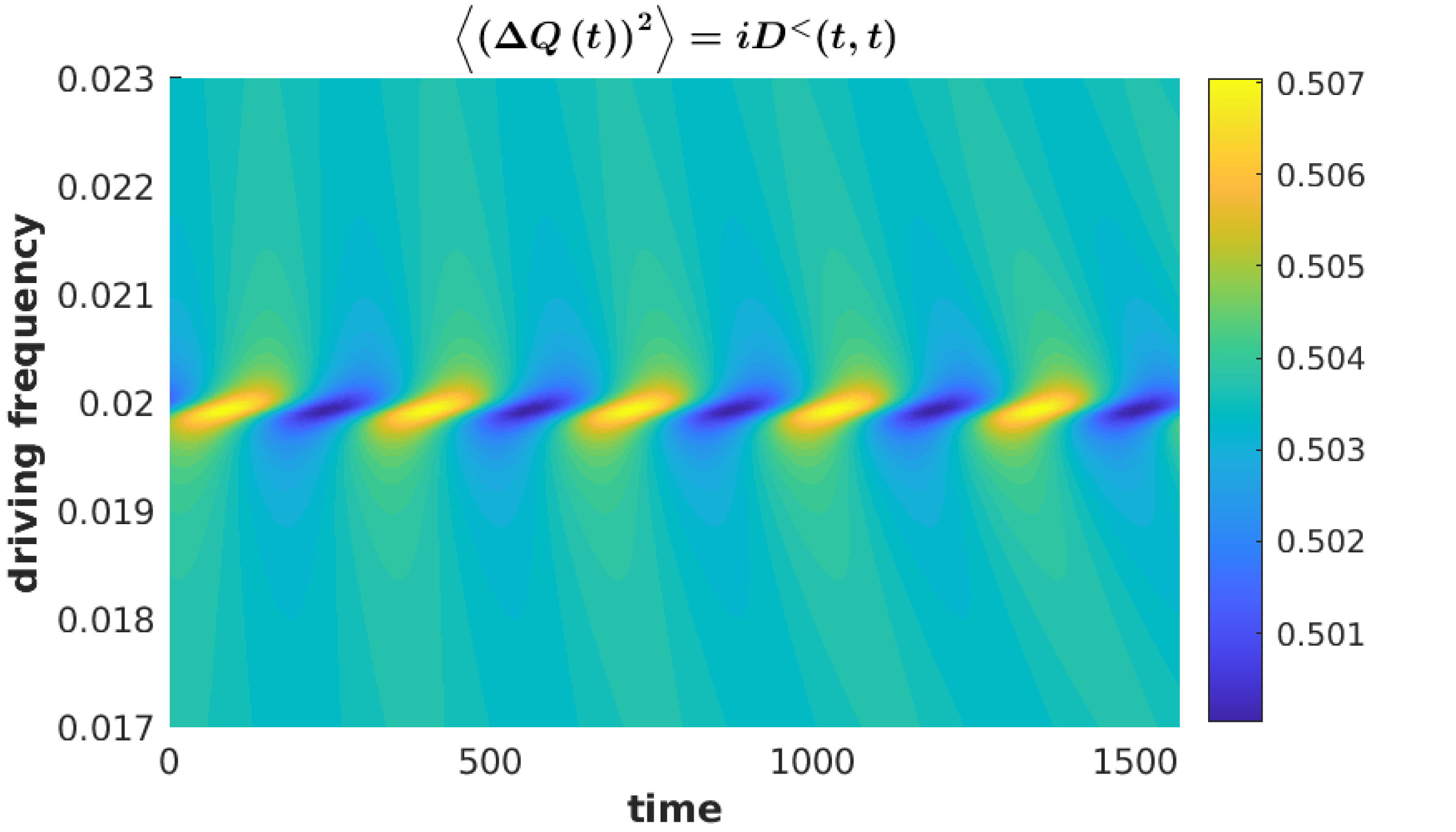
(e)

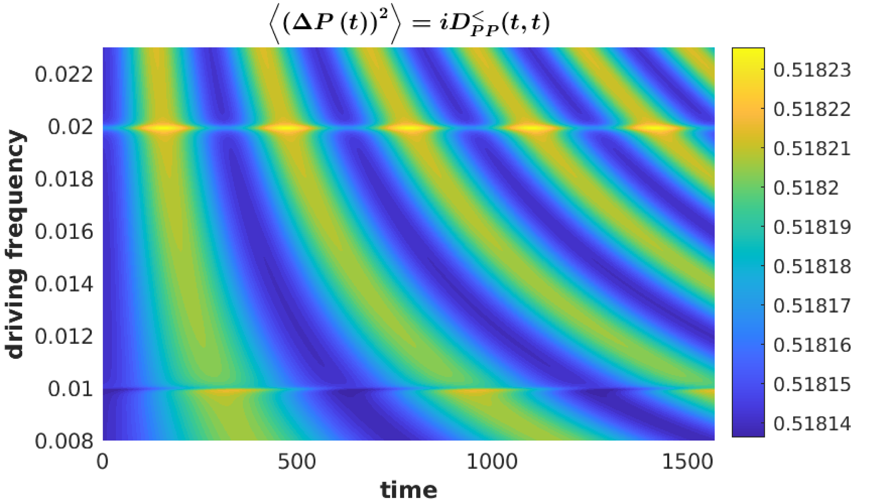
(f)

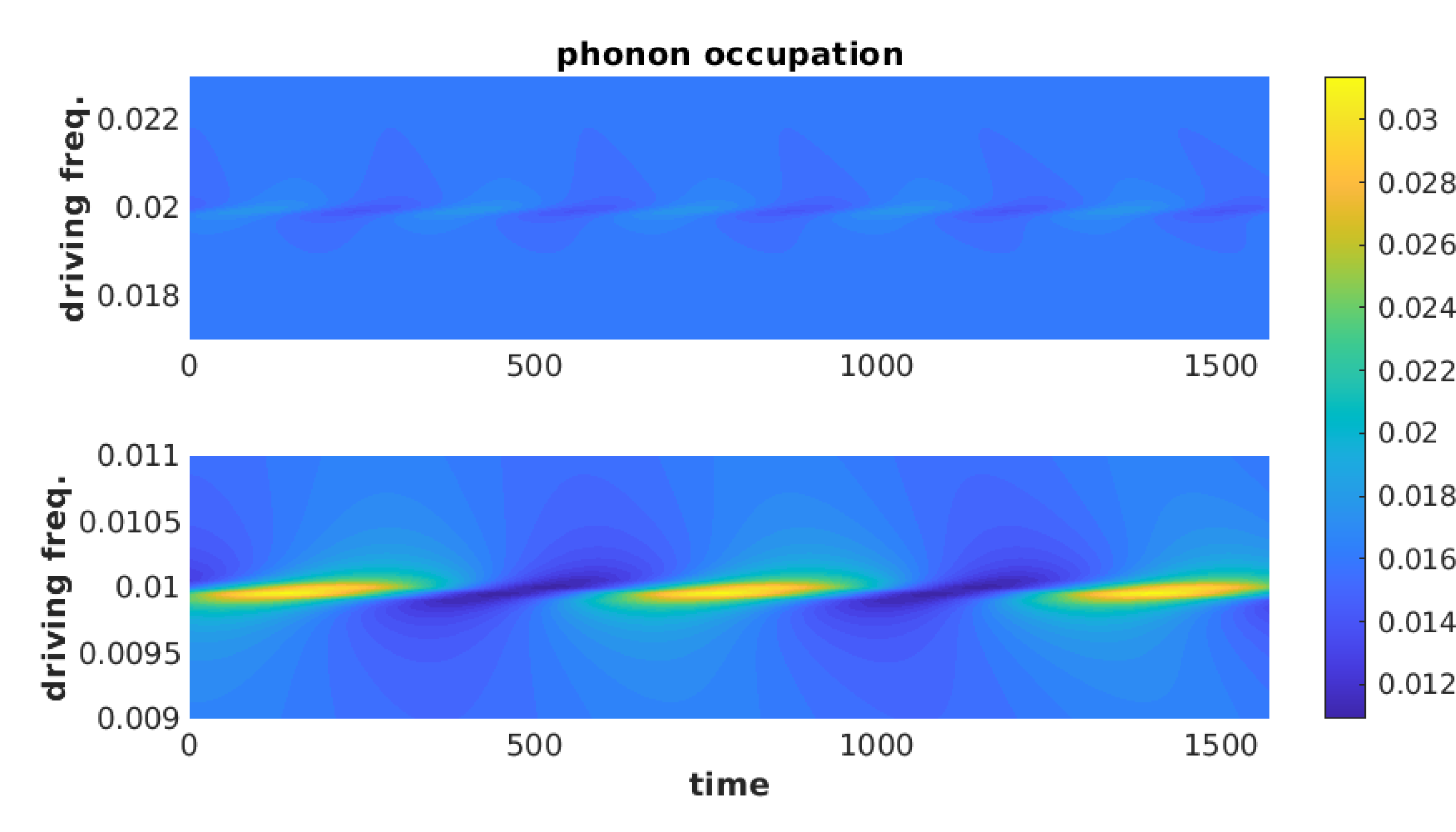
(g)

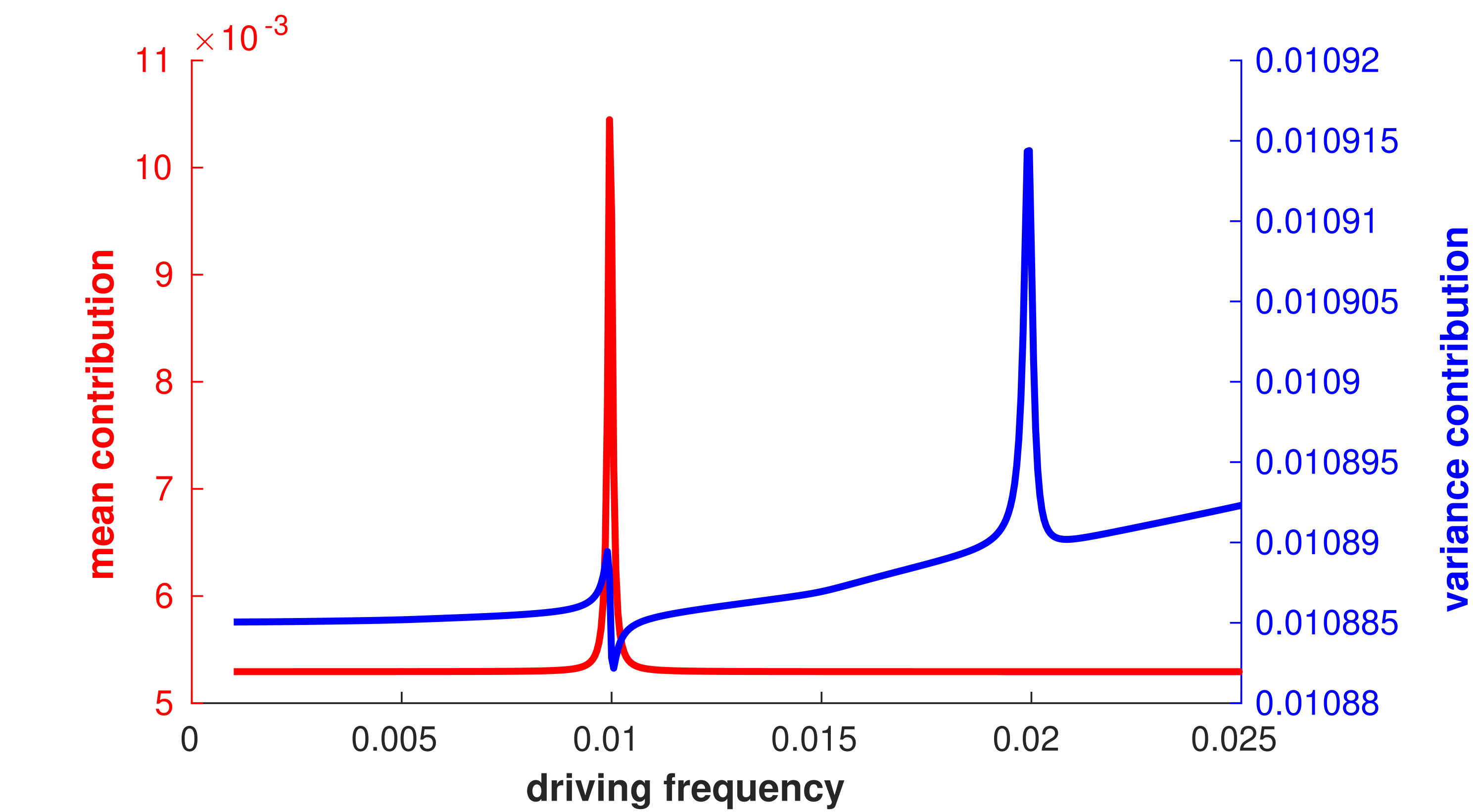
(h)

Figure 3: Figures (a) to (g) plot objects of interest over time, whilst figure (h) plots the time-averaged contributions to the phonon occupation, as given by equation (13). The physical parameters are $\Gamma_{L}=\Gamma_{R}=0.015$, $\epsilon_{c}=0.1$, $T=1.5\times 10^{-4}$, $\omega_{c}=0.01$, $\eta_{c}=6\times 10^{-5}$, $\Delta_{L}=0.0015$ and $\lambda_{c}=0.01$. Fourier coefficients ranging from -14 to 14 were used in the calculation, with an integrand discretization of $2.5\times 10^{-5}$ with bounds of -1 and 1. The convergence was below $10^{-4}$ for both the electronic and phonon occupation.

The above insights suggest a simplistic model where equation (78) is augmented, with the static components being calculated with the addition of electron-phonon interactions. This method was often found to successfully predict the inelastic features of the full model. See figure (2) for an example, where the contributions given by equation (78) are plotted alongside the full and simplistic methods. The convergence for the simplistic model was calculated by using the average occupation as if it were static.

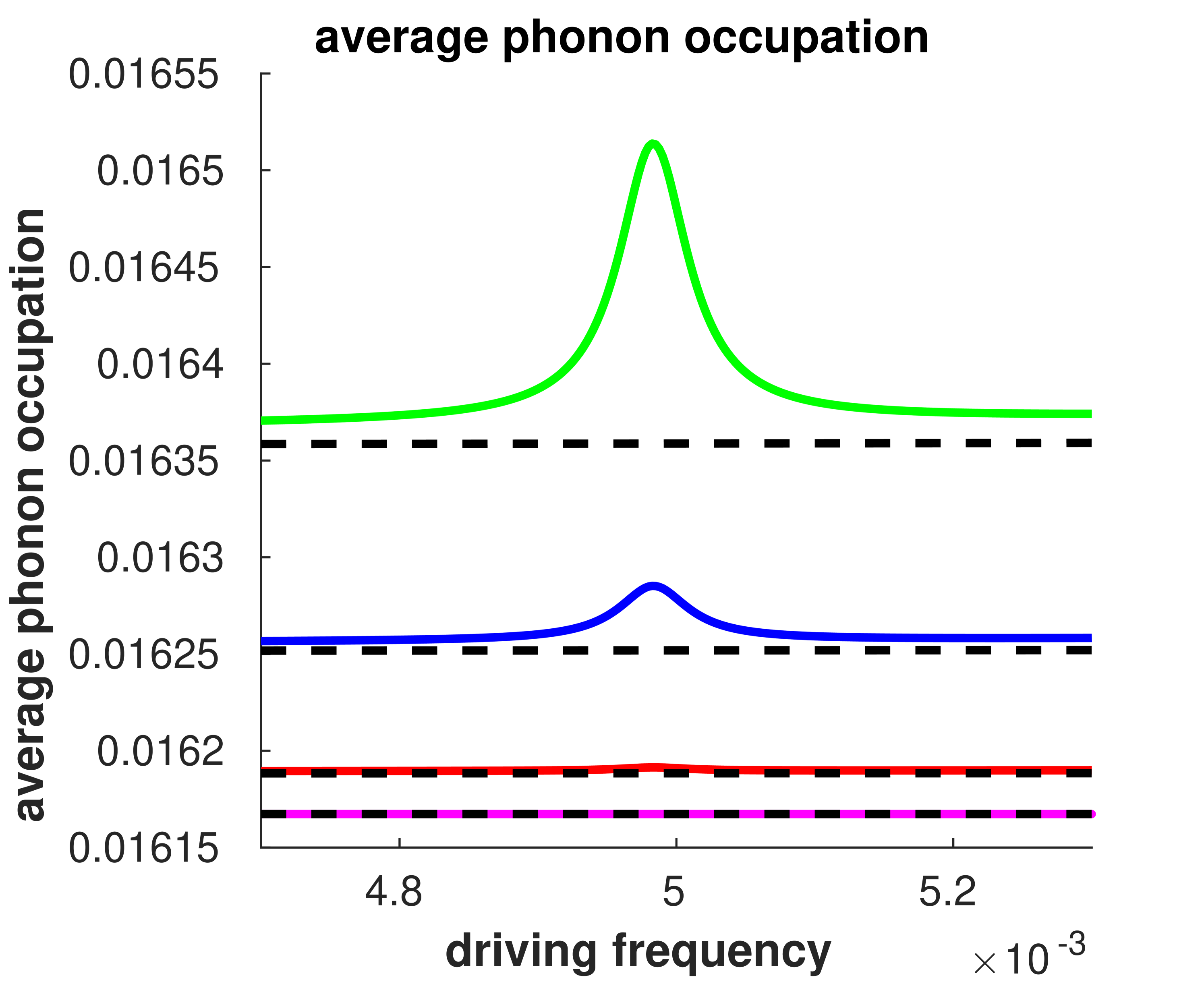
(a)

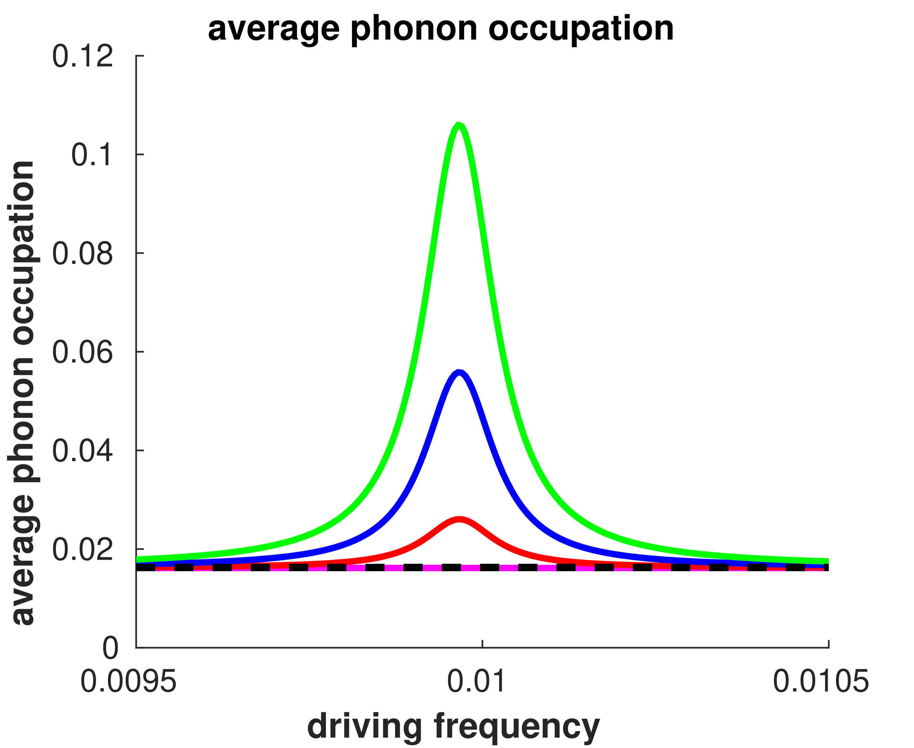
(b)

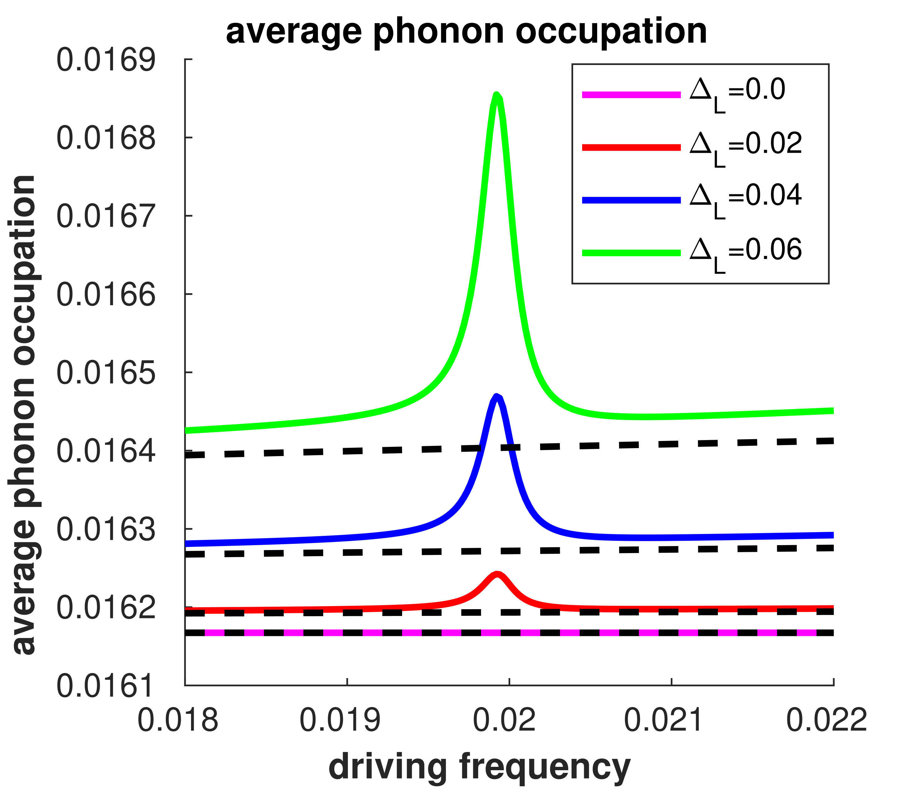
(c)

Figure 4: The time-averaged phonon occupation as driving frequency increases. Here, the driving energies of the left lead, $\Delta_{L}$, have been varied. Furthermore, the simplistic method has been plotted in dashed black. The other parameters are $\Gamma_{L}=\Gamma_{R}=0.015$, $\epsilon_{c}=0.1$, $\eta_{c}=6\times 10^{5}$, $\omega_{c}=0.01$, $\lambda_{c}=0.01$ and $T=1.5\times 10^{-4}$. The bounds of the integrands was taken at -1 and 1. Fourier coefficients ranging from -8 to 8 were used in the calculation. The uniform grid spacing was $5\times 10^{-6}$ for plots (a) and (b) whilst plot (c) was calculated with $1\times 10^{-5}$. The convergence was below $10^{-4}$ for both the electronic and phonon occupation.

The simplistic model can be motivated for situations where the timescales for interaction between the electronic and phononic components, $t_{\lambda}\sim 1/\lambda_{c}$, is far longer than the traversal time for the electrons within the junctioncuevas2010molecular :

$$\frac{1}{\lambda_{c}}\gg\frac{1}{\sqrt{\Gamma^{2}+{\Delta E}^{2}}},$$ (79)

where $\Gamma=\Gamma_{L}+\Gamma_{R}$ and $\Delta E$, the injection energy, is the distance of the energy level from resonance, usually taken as the difference between the energy level and closest chemical potential. In the regime specified by the above assumption, the phonon mode will see the time-dependence of the electronic component averaged over the long interaction time, hence the ability of the simplistic model to capture the dynamics. This insight is similar to that used to investigate the effects of AC driving with master equations Peskin2017 ; Peskin2020 , where weak coupling between central region and leads results in the central region seeing an average picture of the leads’ dynamics.

Within the model in question, it was found that resonance driving at $\Omega\approx\omega_{c}$ resulted in significant variations for several parameter ranges (see figures (3) and (4)). This is mostly due to the sensitivity of average position, to resonant driving, which in turn influences the other observables. This can be seen in figure (3(c)). This sensitivity to resonance comes from equation (73), for which the single level case simplifies to

$$\begin{split}\left\langle Q\right\rangle(m)\\ =\lambda_{c}\;d^{R}\left(-\Omega m\right)n_{el}(m).\end{split}$$ (80)

Focusing on the bare, retarded phonon Green’s function, we can separate out the real and imaginary parts:

$$\begin{split}d^{R}(\omega)=\\ \frac{i}{2}\left(\frac{-\eta_{c}}{\left(\omega-\omega_{c}\right)^{2}+\eta_{c}^{2}}+\frac{\eta_{c}}{\left(\omega+\omega_{c}\right)^{2}+\eta_{c}^{2}}\right)\\ +\frac{1}{2}\left(\frac{\omega-\omega_{c}}{\left(\omega-\omega_{c}\right)^{2}+\eta_{c}^{2}}+\frac{\omega_{c}+\omega}{\left(\omega_{c}+\omega\right)^{2}+\eta_{c}^{2}}\right).\end{split}$$ (81)

The real and imaginary components of above are maximised around $\pm\Omega n\approx\omega_{c}$, especially when the $\eta_{c}\ll\omega_{c}$. This results in the average phonon position being sensitive to periodic variation in the electronic occupation, resulting in the primary resonance peak, seen in figures (3(g)), (3(h)) and (4(b)), around $\Omega\approx\omega_{c}$. Additionally, smaller subharmonic resonances can also be observed, see figures (3(g)) and (4(a)), which indicates the existence of higher order Fourier coefficients in the electronic site’s occupation.

In addition to the resonance at $\Omega\approx\omega_{c}$, a higher, smaller resonance was observed at $\Omega\approx 2\omega_{c}$, see figure (3(e)), (3(f)), (3(g)) and (3(h)). In contrast to resonance at $\Omega\approx\omega_{c}$, the resonance at $\Omega\approx 2\omega_{c}$ is due to increases in the variance of phonon’s position and momentum, which is calculated with the phonon lesser GF. This can be seen in figure (3(h)), where the contributions from equation (13) are separated into the contributions from the mean position and momenta, $\left\langle Q_{\alpha}(t)\right\rangle^{2}+\left\langle P_{\alpha}(t)\right\rangle^{2}$, and the variance terms, $iD^{<}_{\alpha\alpha}\left(t,t\right)+iD^{<,PP}_{\alpha\alpha}\left(t,t\right)$.

Within the parameter ranges investigated, the time-resolved observables were found be explained primarily by the first and second order Fourier coefficients. For the resonances at $\Omega\approx\omega_{c}$ and $\Omega\approx 2\omega_{c}$, the first order Fourier coefficient was the prominent contributor to the time-resolved dynamics. For the subharmonic resonance at $2\Omega\approx\omega_{c}$, the second order Fourier component was found to contribute significantly. This is expected given that this resonance is sensitive to the second order Fourier components within the electronic occupation, as seen in equations (80) and (81).

Figure (4) also shows how the simplistic model fails to capture the resonance effects, whilst still capturing the general trend of the phonon occupation. This is understandable given the simplistic models disregards the driving’s effects on central system’s dynamics.

IV Conclusion

In this work we have investigated the periodic driving of a quantum dot with a Floquet nonequilibrium Green’s function approach and $GD$ approximation. Specifically, the case of sinusoidal driving of the left lead was investigated for a single level and phonon system.

Particularly interesting for the stability of such driven systems, it was found that driving the lead energies in resonance with the vibrational frequency resulted in increased variations in average position, average momentum and occupation of the phonon mode. Moreover, whilst the time-averaged phonon occupation shows an increase in occupation when resonance occurs (see figure (3(h)) and (4)), the time-resolved result (figure (3(g))) reveals more pronounced increases in occupation over the period of driving, reflecting the need to analyse time-resolved results when dealing to periodically driven systems.

Also discussed was a simple, phenomenological model that was found to replicate the time-averaged observables rather well in regimes away from resonance, particularly when the driving frequency was smaller than the vibrational frequency, see figure (2).

The method presented can be extended to many levels, with the addition of extra sites allowing for investigation of models where phonon modes may couple to many electronic sites or to the coupling between sites Park2011 . Furthermore, the effects of different waveforms for the driving could allow for novel means of probing and controlling junction dynamics.

Adding full-counting statistic to the method could allow for the investigation of higher cumulants in the current, including zero-frequency noise Park2011 ; Honeychurch2020 . This could help answer and motivate questions surrounding the noisiness of signals passed through vibrationally active junctions, an important line of inquiry for functional devices. Additionally, statistics surrounding the phononic occupancies may be of importance, with the average occupations not being enough to evaluate the risk of device failure, given the possibility of large variances in occupation.

This study has made use of self-consistent perturbation theory, allowing small electron-vibrational coupling strengths relative to what is present in many junction architectures. Whether the findings of the investigation follow in stronger settings remains to be seen. However, one can hypothesise, that given an increase in electron-vibrational coupling results in more pronounced resonance effects in the present work, the effects of resonance would only become larger in methods able to handle far stronger couplings.

References

• [1] Rani Arielly, Nirit Nachman, Yaroslav Zelinskyy, Volkhard May, and Yoram Selzer. Picosecond time resolved conductance measurements of redox molecular junctions. The Journal of Chemical Physics, 146(9):092306, 2017.
• [2] Jakob Bätge, Amikam Levy, Wenjie Dou, and Michael Thoss. Nonadiabatically driven open quantum systems under out-of-equilibrium conditions: Effect of electron-phonon interaction. Phys. Rev. B, 106:075419, Aug 2022.
• [3] K. Beltako, N. Cavassilas, M. Lannoo, and F. Michelini. Insights into the charge separation dynamics in photoexcited molecular junctions. The Journal of Physical Chemistry C, 123(51):30885–30892, 2019.
• [4] Niels Bode, Silvia Viola Kusminskiy, Reinhold Egger, and Felix von Oppen. Current-induced forces in mesoscopic systems: A scattering-matrix approach. Beilstein Journal of Nanotechnology, 3:144–162, 2012.
• [5] Tobias Brandes. Truncation method for green’s functions in time-dependent fields. Phys. Rev. B, 56:1213–1224, Jul 1997.
• [6] Gabriel Cabra, Ignacio Franco, and Michael Galperin. Optical properties of periodically driven open nonequilibrium quantum systems. The Journal of Chemical Physics, 152(9):094101, 2020.
• [7] J C Cuevas and E Scheer. Molecular Electronics: An Introduction to Theory and Experiment. EBSCO ebook academic collection. World Scientific Publishing Company Pte Limited, 2010.
• [8] L. K. Dash, H. Ness, and R. W. Godby. Nonequilibrium electronic structure of interacting single-molecule nanojunctions: Vertex corrections and polarization effects for the electron-vibron coupling. The Journal of Chemical Physics, 132(10):104113, 2010.
• [9] D Djukic, Kristian Sommer Thygesen, Carlos Untiedt, RHM Smit, Karsten Wedel Jacobsen, and JM Van Ruitenbeek. Stretching dependence of the vibration modes of a single-molecule pt- h 2- pt bridge. Physical Review B, 71(16):161402, 2005.
• [10] A. Erpenbeck, L. Götzendörfer, C. Schinabeck, and M. Thoss. Hierarchical quantum master equation approach to charge transport in molecular junctions with time-dependent molecule-lead coupling strengths. The European Physical Journal Special Topics, 227(15):1981–1994, Mar 2019.
• [11] Michael Galperin, Abraham Nitzan, and Mark A. Ratner. Resonant inelastic tunneling in molecular junctions. Phys. Rev. B, 73:045314, Jan 2006.
• [12] Michael Galperin, Mark A. Ratner, and Abraham Nitzan. Inelastic electron tunneling spectroscopy in molecular junctions: Peaks and dips. The Journal of Chemical Physics, 121(23):11965–11979, 2004.
• [13] Michael Galperin, Mark A. Ratner, and Abraham Nitzan. On the line widths of vibrational features in inelastic electron tunneling spectroscopy. Nano Letters, 4(9):1605–1611, 2004.
• [14] Michael Galperin, Mark A Ratner, and Abraham Nitzan. Molecular transport junctions: vibrational effects. Journal of Physics: Condensed Matter, 19(10):103201, feb 2007.
• [15] H Haug and A P Jauho. Quantum Kinetics in Transport and Optics of Semiconductors, volume 123 of Solid-State Sciences. Springer Berlin Heidelberg, Berlin, Heidelberg, 2008.
• [16] Patrick Haughian, Stefan Walter, Andreas Nunnenkamp, and Thomas L. Schmidt. Lifting the franck-condon blockade in driven quantum dots. Phys. Rev. B, 94:205412, Nov 2016.
• [17] Patrick Haughian, Han Hoe Yap, Jiangbin Gong, and Thomas L. Schmidt. Charge pumping in strongly coupled molecular quantum dots. Phys. Rev. B, 96:195432, Nov 2017.
• [18] Thomas D. Honeychurch and Daniel S. Kosov. Timescale separation solution of the kadanoff-baym equations for quantum transport in time-dependent fields. Phys. Rev. B, 100:245423, Dec 2019.
• [19] Thomas D. Honeychurch and Daniel S. Kosov. Full counting statistics for electron transport in periodically driven quantum dots. Phys. Rev. B, 102:195409, Nov 2020.
• [20] Antti-Pekka Jauho, Ned S. Wingreen, and Yigal Meir. Time-dependent transport in interacting and noninteracting resonant-tunneling systems. Phys. Rev. B, 50:5528–5544, Aug 1994.
• [21] Daniel Karlsson and Robert van Leeuwen. Non-equilibrium Green’s Functions for Coupled Fermion-Boson Systems, pages 367–395. Springer International Publishing, Cham, 2020.
• [22] Yaling Ke, André Erpenbeck, Uri Peskin, and Michael Thoss. Unraveling current-induced dissociation mechanisms in single-molecule junctions. The Journal of Chemical Physics, 154(23):234702, 2021.
• [23] Vincent F. Kershaw and Daniel S. Kosov. Non-adiabatic effects of nuclear motion in quantum transport of electrons: A self-consistent keldysh–langevin study. The Journal of Chemical Physics, 153(15):154101, 2020.
• [24] Maayan Kuperman, Linoy Nagar, and Uri Peskin. Mechanical stabilization of nanoscale conductors by plasmon oscillations. Nano Letters, 20(7):5531–5537, 2020. PMID: 32538634.
• [25] Jing-Tao Lü, Mads Brandbyge, Per Hedegård, Tchavdar N. Todorov, and Daniel Dundas. Current-induced atomic dynamics, instabilities, and raman signals: Quasiclassical langevin equation approach. Phys. Rev. B, 85:245444, Jun 2012.
• [26] Jing-Tao Lü, Mads Brandbyge, and Per Hedegård. Blowing the fuse: Berry’s phase and runaway vibrations in molecular conductors. Nano Letters, 10(5):1657–1663, 2010.
• [27] S. Maier, T. L. Schmidt, and A. Komnik. Charge transfer statistics of a molecular quantum dot with strong electron-phonon interaction. Phys. Rev. B, 83:085401, Feb 2011.
• [28] Maicol A. Ochoa, Yoram Selzer, Uri Peskin, and Michael Galperin. Pump–probe noise spectroscopy of molecular junctions. The Journal of Physical Chemistry Letters, 6(3):470–476, 2015. PMID: 26261965.
• [29] Tae-Ho Park and Michael Galperin. Self-consistent full counting statistics of inelastic transport. Phys. Rev. B, 84:205450, Nov 2011.
• [30] Chandramalika R. Peiris, Simone Ciampi, Essam M. Dief, Jinyang Zhang, Peter J. Canfield, Anton P. Le Brun, Daniel S. Kosov, Jeffrey R. Reimers, and Nadim Darwish. Spontaneous s–si bonding of alkanethiols to si(111)–h: towards si–molecule–si circuits. Chem. Sci., 11:5246–5256, 2020.
• [31] Uri Peskin. Formulation of charge transport in molecular junctions with time-dependent molecule-leads coupling operators. Fortschritte der Physik, 65(6-8):1600048, 2017.
• [32] Gloria Platero and Ramón Aguado. Photon-assisted transport in semiconductor nanostructures. Physics Reports, 395(1):1 – 157, 2004.
• [33] Riley J. Preston, Maxim F. Gelin, and Daniel S. Kosov. First-passage time theory of activated rate chemical processes in electronic molecular junctions. The Journal of Chemical Physics, 154(11):114108, 2021.
• [34] Riley J. Preston, Thomas D. Honeychurch, and Daniel S. Kosov. Cooling molecular electronic junctions by ac current. The Journal of Chemical Physics, 153(12):121102, 2020.
• [35] Riley J Preston, Vincent F Kershaw, and Daniel S Kosov. Current-induced atomic motion, structural instabilities, and negative temperatures on molecule-electrode interfaces in electronic junctions. Physical Review B, 101(15):155415, 2020.
• [36] Jørgen Rammer. Quantum Field Theory of Non-equilibrium States. Cambridge University Press, 2007.
• [37] Michael Ridley, Viveka N. Singh, Emanuel Gull, and Guy Cohen. Numerically exact full counting statistics of the nonequilibrium anderson impurity model. Phys. Rev. B, 97:115109, Mar 2018.
• [38] Michael Ridley, N. Walter Talarico, Daniel Karlsson, Nicola Lo Gullo, and Riku Tuovinen. A many-body approach to transport in quantum systems: From the transient regime to the stationary state. Journal of Physics A: Mathematical and Theoretical, 2022.
• [39] Dmitry A Ryndyk et al. Theory of quantum transport at nanoscale. Springer Series in Solid-State Sciences, 184, 2016.
• [40] C. Schinabeck and M. Thoss. Hierarchical quantum master equation approach to current fluctuations in nonequilibrium charge transport through nanosystems. Phys. Rev. B, 101:075422, Feb 2020.
• [41] M. Schüler, J. Berakdar, and Y. Pavlyukh. Time-dependent many-body treatment of electron-boson dynamics: Application to plasmon-accompanied photoemission. Phys. Rev. B, 93:054303, Feb 2016.
• [42] R. Seoane Souto, R. Avriller, R. C. Monreal, A. Martín-Rodero, and A. Levy Yeyati. Transient dynamics and waiting time distribution of molecular junctions in the polaronic regime. Phys. Rev. B, 92:125435, Sep 2015.
• [43] R. Seoane Souto, A. Levy Yeyati, A. Martín-Rodero, and R. C. Monreal. Dressed tunneling approximation for electronic transport through molecular transistors. Phys. Rev. B, 89:085412, Feb 2014.
• [44] R Seoane Souto, R Avriller, A Levy Yeyati, and A Martín-Rodero. Transient dynamics in interacting nanojunctions within self-consistent perturbation theory. New Journal of Physics, 20(8):083039, aug 2018.
• [45] Gianluca Stefanucci and Robert van Leeuwen. Nonequilibrium Many-Body Theory of Quantum Systems: A Modern Introduction. Cambridge University Press, 2013.
• [46] Niko Säkkinen, Yang Peng, Heiko Appel, and Robert van Leeuwen. Many-body green’s function theory for electron-phonon interactions: Ground state properties of the holstein dimer. The Journal of Chemical Physics, 143(23):234101, 2015.
• [47] Oren Tal, M Krieger, B Leerink, and JM Van Ruitenbeek. Electron-vibration interaction in single-molecule junctions: From contact to tunneling regimes. Physical review letters, 100(19):196804, 2008.
• [48] J. Trasobares, D. Vuillaume, D. Théron, and N. Clément. A 17 ghz molecular rectifier. Nature Communications, 7(1):12850, Oct 2016.
• [49] X. W. Tu, J. H. Lee, and W. Ho. Atomic-scale rectification at microwave frequency. The Journal of Chemical Physics, 124(2):021105, 2006.
• [50] A. Ueda, O. Entin-Wohlman, and A. Aharony. Effects of coupling to vibrational modes on the ac conductance of molecular junctions. Phys. Rev. B, 83:155438, Apr 2011.
• [51] A. Ueda, Y. Utsumi, Y. Tokura, O. Entin-Wohlman, and A. Aharony. Ac transport and full-counting statistics of molecular junctions in the weak electron-vibration coupling regime. J. Chem. Phys., 146(9):092313, 2017.
• [52] Akiko Ueda, Yasuhiro Utsumi, Hiroshi Imamura, and Yasuhiro Tokura. Phonon-induced electron–hole excitation and ac conductance in molecular junction. Journal of the Physical Society of Japan, 85(4):043703, 2016.
• [53] Sifan You, Jing-Tao Lü, Jing Guo, and Ying Jiang. Recent advances in inelastic electron tunneling spectroscopy. Advances in Physics: X, 2(3):907–936, 2017.