The structure of kagome superconductors CsV3Sb5 in the charge density wave states

Abstract

The structure of charge density wave states in AV₃Sb₅ (A = K, Rb, Cs) kagome superconductors remains elusive, with three possible $2a\times 2a\times 2c$ candidates: tri-hexagonal, star-of-David, and their mixture. In this study, we conducted a systematic first-principles investigation of the nuclear quadrupole resonance (NQR) and nuclear magnetic resonance (NMR) spectra for the $2a\times 2a\times 2c$ CsV₃Sb₅ structures. By comparing our simulations with experimental data, we have concluded that the NQR spectrum indicates the tri-hexagonal structure as the proper structure for CsV₃Sb₅ after its charge density wave phase transition. The NMR calculation results obtained from the tri-hexagonal structure are also consistent with the experimental data.

As one of the star materials in condensed matter physics, kagome materials are an important platform for investigating the interplay between correlation, topology, and geometric frustration. The recent discovery of kagome superconductors (SCs), AV₃Sb₅ (A=K,Rb,Cs), has taken the study of kagome physics to a new level Ortiz et al. (2019, 2020, 2021a); Yin et al. (2021); Liang et al. (2021); Chen et al. (2021); Jiang et al. (2021); Nie et al. (2022); Mielke et al. (2022); Jiang et al. (2021); Yu et al. (2021, 2021); Yang et al. (2020); Zhou et al. (2022). Many intriguing phenomena have emerged in AV₃Sb₅, including the anomalous Hall effect (AHE) Yu et al. (2021); Yang et al. (2020); Zhou et al. (2022), pair density wave (PDW) Chen et al. (2021), electronic nematicity Nie et al. (2022), and possible evidence of time-reversal symmetry breaking from muon spin spectroscopy ($\mu$SR) measurements and optical rotation probes Jiang et al. (2021); Mielke et al. (2022); Yu et al. (2021); Feng et al. (2021); Wu et al. (2021); Xu et al. (2022); Park et al. (2021); Denner et al. (2021); Lin and Nandkishore (2021).

In addition to the superconductor transition at $T_{c}$ around 1 $\sim$ 2 K, AV₃Sb₅ also exhibits another structure, a charge density wave (CDW) intertwined with a first-order transition at $T_{s}$ around 80 $\sim$ 100 K Ortiz et al. (2020, 2021a); Yin et al. (2021). Various techniques have been employed to determine the low-temperature structure of AV₃Sb₅, including high-resolution X-ray diffraction (XRD) Li et al. (2021); Miao et al. (2021); Ortiz et al. (2021b, 2020, a); Kautzsch et al. (2023), nuclear magnetic resonance (NMR) and nuclear quadrupole resonance (NQR) Mu et al. (2021); Song et al. (2022); Mu et al. (2022); Luo et al. (2022a), Raman spectroscopy Li et al. (2021), second harmonic generation (SHG) Yu et al. (2021), scanning tunneling microscopy (STM) Jiang et al. (2021); Liang et al. (2021); Zhao et al. (2021), and angle-resolved photoemission spectroscopy (ARPES) Luo et al. (2022b), etc. However, the true structure of AV₃Sb₅ remains controversial, and even similar experimental results can be interpreted in conflicting ways Mu et al. (2022); Luo et al. (2022a). Therefore, theoretical interpretation and numerical simulations of the experiments are urgently needed.

In this study, we systematically investigated the nuclear quadrupole resonance (NQR) and nuclear magnetic resonance (NMR) spectra for various possible structures of AV₃Sb₅ using first-principles calculations. Our simulations generated distinct spectral shapes for a range of structures. By comparing these simulated spectra with experimental measurements, we have identified the tri-hexagonal (TrH) structure as the most likely content, rather than the star-of-David (SoD) structure and the recently proposed SoD-TrH mixture structure.

The pristine AV₃Sb₅ structure is a layered structure of V-Sb sheets intercalated by A atoms with space group $P6/mmm$ Ortiz et al. (2019, 2020), as shown in Fig. 1(a,b). In the V-Sb layer, the V atoms form a standard kagome lattice with additional Sb atoms located at the hexagonal center of the V kagome lattice. Above and below the V-Sb layer, there are two honeycomb lattice planes formed by out-of-plane Sb atoms situated above and below the centers of the V triangles in the kagome plane. The remaining A atoms form another triangular lattice in addition to the above layers.

Using ab initio calculations, two negative energy soft modes were identified around the M and L points in the phonon spectrum Tan et al. (2021); Christensen et al. (2021); Ptok et al. (2022). Based on the vibration pattern of these soft modes, two possible distorted structures for the V layers were proposed: the tri-hexagonal (TrH) and star-of-David (SoD) patterns Tan et al. (2021); Christensen et al. (2021); Ptok et al. (2022). In the SoD structure, V atoms are shrunk into a star-of-David or hexagram pattern, as shown in Fig. 1(c). The TrH structure, on the other hand, consists of two different components: small triangles and large hexagons, as illustrated in Fig. 1(d). The small triangles form a honeycomb lattice, while the large hexagons form a triangular lattice. Both distortions enlarge the unit cell to a $2a\times 2a$ unit cell, as experimentally confirmed Jiang et al. (2021); Li et al. (2021); Miao et al. (2021); Ortiz et al. (2021b); Kautzsch et al. (2023). From a point group perspective, both structures still have the D_6h point group. Therefore, experimental techniques based on symmetry principles cannot directly differentiate between them. However, NQR and NMR, which probe the local environment of the atoms, provides a unique way to determine the structure of AV₃Sb₅.

In addition to the in-plane distortion, AV₃Sb₅ also undergoes a transition along the $c$-direction. The structural transitions in KV3Sb5 and RbV3Sb5 have been experimentally confirmed to be $2a\times 2a\times 2c$ Jiang et al. (2021); Li et al. (2021). However, the structure of CsV3Sb5 is still under debate, with proposed structures of $2a\times 2a\times 2c$ or $2a\times 2a\times 4c$ Li et al. (2021); Miao et al. (2021); Ortiz et al. (2021b); Kautzsch et al. (2023). Since our calculations cannot settle this debate, we will focus only on the $2a\times 2a\times 2c$ structure in our discussion. Within this scope, we will use Cs as an example. We also performed NQR calculations for K and Rb (Tab. S9-S12), and find that the different alkali metal atoms does not impact our main results. With various proposals, we can construct three $2a\times 2a\times 2c$ structures: TrH/TrH, SoD/SoD, and TrH/SoD mixture, as illustrated in Fig. 1(e)-(g). In all the cases, we shift the $C_{6}$ center by one lattice constant to fulfill the $2c$ modulation between each layer. In the following discussion, we will only label them as TrH, SoD and Mix to simplify our notations.

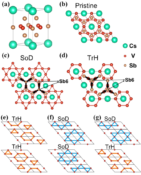
Figure 1: (a) Axonometric view of the pristine crystal structure of CsV3Sb5. (b) Top view of the pristine crystal structure.(c) Top view of the $2a\times 2a$ SoD structure. (d) Top view of the $2a\times 2a$ TrH structure. The moving directions of the three V atoms directly below Sb6 are also shown in (c),(d). (e) $2a\times 2a\times 2c$ pure TrH. (f) $2a\times 2a\times 2c$ pure SoD. (g) $2a\times 2a\times 2c$ TrH/SoD mix structure. Only the V kagome layer is shown in figures (e)-(g).

In NQR and NMR spectra, the number, height, and position of peaks are key pieces of information for determining the crystal structure. The number of peaks reflects how many kinds of non-equivalent atoms are present in the material. The ratio of the heights of the peaks should be exactly equal to the ratio of the number of each kind of atom. The positions of the peaks reflect the local structural information of each kind of atom in the material. Therefore, a systematic analysis of the crystal structure is first needed.

Due to the distortion in the $c$-direction, the six-fold rotation symmetry is broken. The pure TrH and pure SoD bilayer structures belong to space group $Fmmm$, while the Mix structure belongs to space group $Cmmm$. In the pristine structure above $T_{s}$, the three V atoms are equivalent, while the five Sb atoms are divided into two groups: one in-plane Sb1 atom and four out-of-plane Sb2 atoms.

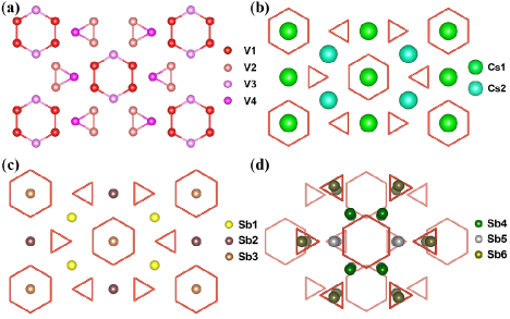
Figure 2: Non-equivalent atoms of TrH. (a) Non-equivalent V atoms. (b) Non-equivalent Cs atoms. (c),(d) Non-equivalent Sb atoms. In order to make the figures clear, in figure (a), only one V kagome plane is shown, in figure (b), only one V kagome plane and the closest Cs plane are shown, in figure (c), only one V kagome plane and Sb1-3 atoms in the plane are shown, in figure (d), only two V kagome planes and Sb4-6 atoms adjacent to the upper V kagome plane are shown.

After the charge density wave phase transition, the equivalent class of atoms in AV₃Sb₅ largely changes. In the $2a\times 2a\times 2c$ TrH structure, there are two types of Cs atoms, four types of V atoms, and six types of Sb atoms (as shown in Fig. 2 and Fig. S2(a)). The ratio of Cs atoms is Cs1:Cs2=1:1, while the ratio of V atoms is V1:V2:V3:V4=2:2:1:1, and the ratio of Sb atoms becomes Sb1:Sb2:Sb3:Sb4:Sb5:Sb6=2:1:1:8:4:4. V1 and V3 belong to the large hexagon, while V2 and V4 belong to the triangle in the TrH configuration. Sb1, Sb2, and Sb3 are located in the kagome plane and derive from Sb1 in the pristine structure, while Sb4, Sb5, and Sb6 are out of the plane and derive from Sb2 in the pristine structure. Sb4 and Sb5 are next to the hexagon, and Sb5 is directly above the V-triangle. Sb6 is also directly above the triangle, but it is much closer than Sb5.

In the $2a\times 2a\times 2c$ SoD structure, the situation is the same as TrH (as shown in Fig. S2(b)). Despite the size of the distortion, the only difference between the two structures is that the displacement direction of all V atoms in SoD is opposite to that in TrH Tan et al. (2021). For the $2a\times 2a\times 2c$ Mix structure, the pattern of adjacent kagome planes is different. Hence, there are more different kinds of non-equivalent atoms than TrH and SoD. For Cs atoms, the number becomes three. For V and Sb, these numbers are doubled (as shown in Fig. S2(c)). The ratio of Cs atoms becomes Cs1:Cs2:Cs3=1:2:1. For V atoms, this ratio is V1:V2:V3:V4:V5:V6:V7:V8=2:2:1:1:2:2:1:1, and for Sb atoms, the ratio is Sb1:Sb2:Sb3:Sb4:Sb5: Sb6:Sb7:Sb8:Sb9:Sb10:Sb11:Sb12=2:1:1:8:4:4:2:1:1:8:4:4.

Equipped with the above information, we can now present our computational results of the NQR spectra and compare them with the experimental results Mu et al. (2022); Luo et al. (2022a). The elementary principle of NQR is based on the electric quadrupole moment $Q$ of the nucleus. This quadrupole moment arises from the non-spherical charge distribution of a nucleus with a spin quantum number $I$ greater than 1/2 Suits (2006). The quadrupole moment couples to the electric field gradient generated by the electronic bonds in the surrounding environment, resulting in the splitting of the nucleus energies. These energy splittings can be detected through radio-frequency (RF) magnetic fields, as in NMR spectroscopy Suits (2006). Therefore, NQR can be utilized to determine the distortion in the crystal structure.

The quadrupole interaction is described by an effective Hamiltonian Slichter (1996):

$$H_{Q}=\frac{eQV_{zz}}{4I(2I-1)}[(3I_{z}^{2}-I^{2})+\frac{1}{2}\eta(I_{+}^{2}+I_{-}^{2})],$$ (1)

where $V_{zz}$ is defined as the maximum eigenvalue of the electric field gradient tensor, and $\eta=\lvert({V_{xx}-V_{yy}})/{V_{zz}}\rvert$ is the asymmetry parameter. We focus on the experimentally available ^121Sb in the NQR spectra. For ^121Sb, $Q=$-54.3\text{\times}{10}^{-30}\text{\,}\mathrm{m}^{2}$$ and $I=5/2$. Since $I=5/2$, two peaks can be detected experimentally for each kind of non-equivalent Sb atom, belonging to $\ket{\pm 1/2}\leftrightarrow\ket{\pm 3/2}$ and $\ket{\pm 3/2}\leftrightarrow\ket{\pm 5/2}$ transitions. Here, we only consider the transition $\ket{\pm 1/2}\leftrightarrow\ket{\pm 3/2}$.

Another important quantity in NQR is the quadrupole resonance frequency $\nu_{Q}$, which is defined as $\nu_{Q}=\frac{3eQV_{zz}}{2I(2I-1)h}$ Slichter (1996). The energy difference between the two states is denoted as $\Delta E$, and $f$ satisfies $hf=\Delta E$ corresponding to the frequency. When $\eta=0$, the absolute value of the quadrupole resonance frequency is equal to the frequency corresponding to the transition $\ket{\pm 1/2}\leftrightarrow\ket{\pm 3/2}$. However, in most cases, $\eta$ is a small value, and second-order perturbation theory can be used to calculate $f$ when $\eta\neq 0$ (see Appendix):

$$f=\left(1+\frac{59}{54}\eta^{2}\right)|\nu_{Q}|.$$ (2)

For the first-principles calculations, we utilize the all-electron augmented plane wave (APW) basis set Martin (2020); Singh and Nordstrom (2006); Sjöstedt et al. (2000) implemented in the WIEN2k package Blaha et al. (2020). The NQR calculation in WIEN2k is described in Chapter 6.4 of reference Schwarz et al. (2010).

We found that the calculated NQR spectra for the four different crystal structures in Fig. 1(a),(e)-(g) depend on the lattice parameters and the the lengths of each chemical bond in each structure. However, we need to point out that the main feature used to distinguish SoD from TrH does not depend on these factors, which will be discussed later. Therefore, we first need to find suitable crystal structures. For the undistorted pristine structure, we used the experimental structure. For the three candidate distorted structures, since there are no completely uncontroversial experimental data available, one option is to use the optimized results from density functional theory (DFT) calculations. The DFT structure optimization test showed that the lattice parameters in the kagome plane hardly changed (less than $0.01\AA$ compared to twice the undistorted experimental values), and the lattice parameter in the direction perpendicular to the plane did not change much (less than $0.05\AA$ compared to twice the undistorted experimental values). Therefore, as a reliable approximation, we took the lattice parameters of these three $2a\times 2a\times 2c$ structures to be twice the undistorted experimental values, and then optimized the internal coordinates. In the main text, we used the relaxed crystal structures to calculate the NQR spectra, which are shown in Fig. 3(b)-(d). We then compared them with the experimental results Mu et al. (2022) (See Fig. 3(a)). Recently, another study also provided some experimental refined structure models using single-crystal X-ray crystallographic refinements Kautzsch et al. (2023). These experimental structures were also used to calculate the NQR parameters, which are shown in Tab. S5-S6. The results for the pristine structure are shown in Fig. S1(a,b). All the detailed data, including $V_{zz}$, $\nu_{Q}$, and $\eta$, can be found in the Appendix. In Fig. 3 and Fig. S1, the calculated data were broadened using the following Lorentzian function:

$$y=\frac{2}{\pi}\frac{w}{4(x-x_{c})^{2}+w^{2}},$$ (3)

where $w=\frac{2}{\pi y_{c}}$ and ($x_{c}$,$y_{c}$) is the coordinate of the top of the Lorentzian peak. Here, $x_{c}$ is the frequency and $y_{c}$ is the intensity, which is proportional to the number of atoms.

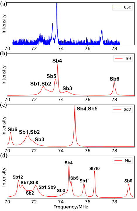
Figure 3: The NQR spectra for experimental and calculated results. (a) Experimental spectrum at 85K (below $T_{s}$) Mu et al. (2022). (b) Calculated spectrum of relaxed $2a\times 2a\times 2c$ TrH. (c) Calculated spectrum of relaxed $2a\times 2a\times 2c$ SoD. (d) Calculated spectrum of relaxed $2a\times 2a\times 2c$ mixture structure. For comparison purposes, the calculated results are shifted by +4.7 MHz.

As shown in Fig. 3, the NQR spectrum of the $2a\times 2a\times 2c$ TrH structure exhibits a closer match to the experimental results, albeit with a constant frequency shift. However, it’s important to note that the decision to exclude the other two structures was not solely based on the resemblance between the calculated and experimental spectra. Here, we will first examine the main distinguishing feature in the calculated NQR spectra of TrH and SoD, which is insensitive to lattice parameters and specific atomic positions. Based on this feature, we will then determine which type of NQR spectrum the experimental results belong to.

The main distinguishing feature between the calculated NQR spectra of TrH and SoD is the relative positions of the Sb4, Sb5, and Sb6 peaks, all of which arise from Sb2 in the pristine structure. These three kinds of Sb atoms are located outside the kagome plane, with each Sb atom having three nearest neighboring V atoms inside the adjacent kagome plane. In TrH, the Sb6 peak appears at a higher frequency than Sb4 and Sb5 (Fig. 3(b)). On the other hand, for SoD, the situation is reversed (Fig. 3(c)). This difference can be explained by the displacement directions of the three V atoms closest to Sb6. In TrH, the three V atoms are closer to Sb6 and form a triangle (Fig. 1(d) and Fig. 2(d)), whereas in SoD, the three V atoms are further away from Sb6 (Fig. 1(c)). However, for any Sb4 or Sb5 atom, two of the three V atoms move in a direction perpendicular to the V-Sb bond. Therefore, in the TrH structure, Sb6 experiences a larger electric field gradient than Sb4 and Sb5, resulting in a higher frequency of the Sb6 peak than the Sb4 and Sb5 peaks. In contrast, in the SoD structure, Sb6 experiences a smaller electric field gradient than Sb4 and Sb5, resulting in a lower frequency of the Sb6 peak than the Sb4 and Sb5 peaks. This result is caused by the inherent characteristics of the two structures and does not depend on lattice parameters or bond lengths. For both optimized DFT structures , experimental structures and other structures, this result can be observed (See Appendix). To further confirm the effect of the displacements of the three closest V atoms on the position of the Sb6 peak in the NQR spectra, we fixed the displacement of other V atoms and only varied the displacements of V atoms closest to Sb6. As expect, our results show that when the displacement of V atoms is greater (closer to Sb6), the Sb6 peak shifts to a higher frequency (Tab. S7).

After analyzing the computational results, we need to determine which case the experimental NQR spectrum corresponds to. This requires us to be able to assign the peaks in the experimental results to the corresponding Sb atoms, especially Sb4, Sb5, and Sb6. Here, we will use the more convincing indicators of peak height and asymmetry parameters ($\eta$) to accomplish this task. The calculated $\eta$ for both TrH and SoD are shown in Tab. 1, while the experimental results are listed in Tab. 2. Based on the number of atoms and the $\eta$ values, we determine that the highest peak and its adjacent peak (peak 3 and peak 2 in Tab. 2) in Fig. 3(a) should originate from Sb4 and Sb5. In previous experimental reports, the peak with the highest frequency ($\sim$ 77 MHz in Fig. 3(a), peak 4 in Tab. 2) has been considered to originate from Sb1-Sb3 which all arise from Sb1 in pristine structure due to its close-to-zero $\eta$ Mu et al. (2022); Luo et al. (2022a). Here, we argue that this peak should not come from Sb1-Sb3. From the calculation results of DFT relaxed structures, only Sb3 and Sb6 satisfy the condition of $\eta$ equals to zero. However, the proportion of Sb3 is only 1/8 of Sb4, so it cannot produce such a high peak. Regarding the experimental structure reported in Ref.Kautzsch et al. (2023), the computational results indicate that only the Sb6 peak has a $\eta$ value close to zero (see Tab. 1 or Tab. S5-S6). In conclusion, this peak is more likely to originate from Sb6. Consequently, since the frequency of the Sb6 peak is higher than that of the Sb4 and Sb5 peaks in the experimental spectrum, we believe that TrH is a more plausible structure than SoD.

Finally, the calculated NQR spectrum of the Mix structure is simply a superposition of those of TrH and SoD (see Fig. 3(d)). Thus, based solely on the number of peaks, Mix does not seem to be a suitable structure.

Table 1: Asymmetry parameters $\eta$ for Sb atoms in calculated NQR speatra.

	Sb1	Sb2	Sb3	Sb4	Sb5	Sb6
Cal.(pristine)	0	0	-	-	-	-
Cal.(relaxed TrH)	0.069	0.068	0	0.129	0.131	0.003
Cal.(relaxed SoD)	0.045	0.047	0	0.093	0.09	0
Cal.(exp. TrHKautzsch et al. (2023))	0.035	0.022	0.037	0.04	0.039	0.007
Cal.(exp. SoDKautzsch et al. (2023))	0.036	0.022	0.038	0.035	0.041	0.001

Table 2: Asymmetry parameters $\eta$ for Sb atoms in experimental NQR speatra. The frequency of the peak increases from left to right.

	Peak1	Peak2	Peak3	Peak4
Exp.(95K)Mu et al. (2022)	0	0	-	-
Exp.(85K)Mu et al. (2022)	0.04	0.07	0.07	0

To further support the conclusion that the CDW pattern below $T_{s}$ corresponds to TrH, we calculated the NMR knight shifts of Cs and V and compared them with experimental results Mu et al. (2021); Song et al. (2022).

When a uniform external magnetic field $\textbf{B}_{\textbf{ext}}$ is applied, the nuclear magnetic moments interact with it, which results in the nuclear Zeeman effect. The electron magnetic moments also interact with the nuclear magnetic moments, inducing an effective magnetic field $\textbf{B}_{\textbf{ind}}(\textbf{R})$ at position R. When $\textbf{B}_{\textbf{ext}}$ is not very strong, the relationship between the two fields is linear, given by:

$$\textbf{B}_{\textbf{ind}}(\textbf{R})=K(\textbf{R})\textbf{B}_{\textbf{ext}},$$ (4)

where $K$ is known as the NMR knight shift tensor and can be divided into the orbital and spin parts Slichter (1996), corresponding to the electron orbital magnetic moment and the electron spin magnetic moment, respectively. In experimental measurements, the external magnetic field is applied perpendicular to the kagome plane, along the $z$ direction. Hence, the experimental knight shift data corresponds to the $K_{zz}$ component. The experimental and calculated NMR knight shift values $K_{zz}$ are presented in Tab. 3.

Compared to NQR, the NMR knight shift is more sensitive to the crystal structure. Our tests show that even a slight change in the V-V bond length can lead to a large change in the spin part of the knight shift, resulting in significant deviation from experimental results. Therefore, a relaxed crystal structure that still has a certain gap with the real structure is not suitable for NMR calculation. We either use the experimental $2a\times 2a\times 2c$ TrH structure in ref Kautzsch et al. (2023) or manually adjust the distortion. The results of the experimental structure are shown in Tab. S13. We find that the calculated NMR knight shift values are very close to the experimental values Song et al. (2022); Mu et al. (2021), but four different peaks appear, which is inconsistent with the experimental result that only has two peaks. Hence, we also try to use manually tuned structures in NMR calculations. Unlike the experimental structure, we keep the hexagons as regular hexagons and the triangles as regular triangles, although the space group symmetry of the crystal does not guarantee this. For example, in Tab. 3, we list the results for 0.01-0.01 TrH. The first 0.01 represents the displacement of the V atoms that make up the hexagons, and the second 0.01 represents the displacement of the V atoms that make up the triangles, and the unit is angstrom. The NMR results of some other manually tuned structures are shown in Tab. S14. For the DFT relaxed structure, the distortion is around 0.045-0.08.

In order to maintain consistency of the structures used for NMR and NQR calculations, the manually tuned structure 0.01-0.01 TrH is also used to calculate the NQR spectra (See Tab. S8 and Fig. S1(c,d)). As expected, this structure gives the same result like the DFT relaxed TrH structure.

Table 3: NMR knight shift $K_{zz}$ for Cs and V atoms in pristine and manually adjusted 0.01-0.01 TrH structures. The first 0.01 represents that the displacement of the V atoms that make up the hexagon is 0.01Å, and the second 0.01 represents the displacement of the V atoms that make up the triangle is also 0.01Å.

	Cs1	Cs2	V1	V2	V3	V4
Exp.(95K)Song et al. (2022); Mu et al. (2021)/ppm	3300	-	4000	-	-	-
Cal.(Pristine)/ppm	2745	-	3856	-	-	-
Exp.(93K)Song et al. (2022); Mu et al. (2021)/ppm	3400	2250	3700	4200	-	-
Cal.(0.01-0.01TrH)/ppm	3107	2514	3811	4030	3823	4071

One important point to note is that the $2a\times 2a\times 2c$ TrH crystal structure contains four types of non-equivalent V atoms, yet only two NMR peaks were experimentally observed below $T_{s}$. The NMR calculation results of the experimental structure reported in ref Kautzsch et al. (2023) do not lead to this conclusion. However, from the calculated results of manually tuned structures, the four V atoms can be divided into two groups: one group consists of V1 and V3, which belong to the hexagon, while the other group consists of V2 and V4, which belong to the triangle. The knight shifts for each group are so close that they cannot be distinguished in experiments, resulting in only two distinct NMR peaks being observed.

From Tab. 3 and Tab. 4, we can see that the calculated NMR knight shift values using manually tuned structures are very close to the experimental NMR results Song et al. (2022); Mu et al. (2021). The pristine structure used in the calculation is the experimental structure, and the calculated knight shift values are also close to the experimental values. Therefore, we have reason to believe that the real CDW structure has V atom displacements ranging from about 0.01$\AA$ to 0.015$\AA$ in both hexagons and triangles, or V-V bond lengths of about 2.735$\AA$ in hexagons and 2.725$\AA$ in triangles. Notably, the experimental $2a\times 2a\times 2c$ TrH structure in ref Kautzsch et al. (2023) has V-V bond lengths very close to those we have proposed here.

For both pristine and representative 0.01-0.01 TrH structures, the total NMR Knight shift is decomposed into the orbital term, spin Fermi contact term, and spin dipolar term. The detailed values are presented in Tab. 4. From Tab. 4, it is evident that the main contribution to the NMR knight shift for Cs atoms is the spin Fermi contact term, which may be due to the large paramagnetic contribution from the spin-polarized valence s electrons of Cs. However, for V atoms, the main contribution comes from the orbital term, which is also consistent with the experimental findings Song et al. (2022). It is worth noting that the spin contact term is diamagnetic for V atoms, which is uncommon except for transition metal elements. This is due to the external magnetic field inducing a sizable V 3d spin-magnetic moment, which introduces a large core polarization of opposite sign Laskowski and Blaha (2015); Ebert et al. (1986). Because of the anisotropy of the crystal field for V atoms, the spin dipolar term also has a significant contribution mainly from V 3d electrons. Overall, our NMR calculations also support the TrH as the correct CDW structure below $T_{s}$.

Table 4: Decomposition NMR knight shift into orbital term($K_{o}$), spin Fermi contact term($K_{fc}$), and spin dipolar($K_{sd}$) term for pristine and 0.01-0.01 TrH structures.

	$K_{o}$	$K_{fc}$	$K_{sd}$	Total
Pristine-Cs1/ppm	-5318	8118	-55	2745
Pristine-V1/ppm	5613	-2366	609	3856
TrH-Cs1/ppm	-5276	8395	-12	3107
TrH-Cs2/ppm	-5293	7859	-52	2514
TrH-V1/ppm	5644	-2390	557	3811
TrH-V2/ppm	5743	-2245	532	4030
TrH-V3/ppm	5635	-2406	593	3822
TrH-V4/ppm	5753	-2288	606	4071

In summary, we conducted a systematic first-principles study of CsV3Sb5 using NQR and NMR spectroscopy. We considered three possible $2a\times 2a\times 2c$ structures, TrH, SoD, Mix, and the pristine structure to obtain ¹²¹Sb NQR spectra by calculating the NQR electric field gradients and asymmetry parameters. The main feature in ¹²¹Sb NQR spectra is determined by the relative positions of the Sb4 and Sb5 peaks to the Sb6 peak, which all come from Sb2 in the pristine structure. Comparing our results with experimental measurements Mu et al. (2022); Luo et al. (2022a), we conclude that the TrH structure is more likely to be the correct structure. To further confirm this result, we calculated the NMR knight shift for the TrH structure and the pristine structure. Although the TrH structure has four non-equivalent V atoms, if the hexagons and triangles mentioned are regular hexagons and equilateral triangles, respectively, they can be divided into two groups based on whether they belong to the hexagon or triangle. Within each group, two kinds of V atoms have a very close knight shift, which can account for only two V NMR peaks appearing in the experiments below $T_{s}$ Song et al. (2022); Mu et al. (2021). Therefore, our calculations demonstrate that within the $2a\times 2a\times 2c$ range, TrH should be the right structure below $T_{s}$ for CsV3Sb5, and possibly for all AV3Sb5 materials, but not the SoD Luo et al. (2022a) or the coexistence of TrH and SoD Ortiz et al. (2021b); Wu et al. (2022). We also want to mention that our calculations do not settle the debate between $2a\times 2a\times 2c$ and $2a\times 2a\times 4c$ in CsV3Sb5 Miao et al. (2021); Ortiz et al. (2021b); Kautzsch et al. (2023); Xiao et al. (2022), which requires further investigation.

Note that, when finalizing this work, we became aware of another work working on RbV3Sb5 with similar results Frassineti et al. (2022).

This work is supported by the National Natural Science Foundation of China (Grant No. NSFC-11888101, No. NSFC-12174428), the Strategic Priority Research Program of Chinese Academy of Sciences (Grant No. XDB28000000), and the Chinese Academy of Sciences through the Youth Innovation Promotion Association (Grant No. 2022YSBR-048).

Appendix

Appendix A THEORETICAL APPROACH

A.1 NQR

Here, we will outline the basic theory for calculating the relevant parameters of nuclear quadrupole resonance (NQR), such as the electric field gradient $V_{zz}$ and the asymmetry parameter $\eta$ Slichter (1996). When we do not consider the nucleus as a point charge, the nucleus in different states will have different interaction energies with the external potential field under the same external potential field. Classically, the interaction energy $E$ of a charged nucleus with a charge density $\rho(\textbf{r})$ with an external potential $V(\textbf{r})$ can be described as:

$$E=\int\rho(\textbf{r})V(\textbf{r})d^{3}r.$$ (5)

We expand $V(\textbf{r})$ to second order in a Taylor’s series about the origin:

$$V(\textbf{r})=V(\textbf{0})+\textbf{r}\cdot\nabla V\mid_{\textbf{r}=\textbf{0}}+\frac{1}{2}\sum_{i,j=1}^{3}x_{i}x_{j}\frac{\partial^{2}V}{\partial x_{i}\partial x_{j}}\mid_{\textbf{r}=\textbf{0}}.$$ (6)

We set the position of a nucleus as the origin. When we put equation 6 into equation 5,the first order term $\int\rho(\textbf{r})\textbf{r}\cdot\nabla V\mid_{\textbf{r}=\textbf{0}}d^{3}r$ vanishes if the nuclear states possess the definite parity. Fortunately, all experimental evidence supports this contention.

It is convenient to define another quantities $Q_{ij}$:

$$Q_{ij}=\int(3x_{i}x_{j}-\delta_{ij}r^{2})\rho(\textbf{r})d^{3}r.$$ (7)

The external potential must satisfy Laplace equation:$\nabla^{2}V=0$. Defining $\frac{\partial^{2}V}{\partial x_{i}\partial x_{j}}\mid_{\textbf{r}=\textbf{0}}=V_{ij}$, the second order term,which is also called the quadurpole energy $E^{(2)}$, is given by:

$$E^{(2)}=\frac{1}{6}\sum_{i,j=1}^{3}V_{ij}Q_{ij}.$$ (8)

It can be quantized by replacing the charge density $\rho(\textbf{r})$ with the corresponding quantum mechanical operator:

$$\rho(\textbf{r})=e\sum_{k}\delta(\textbf{r}-\textbf{r}_{\textbf{k}}).$$ (9)

Summing over k here means summing over all protons, because we no longer think of nuclei as point charges. In the subspace formed by the total angular momentum eigenstates of the nucleus, using Wigner-Eckart theorem, the quadrupole energy can be described by an effective hamiltonian:

$$H_{Q}=\frac{eQV_{zz}}{4I(2I-1)}[(3I_{z}^{2}-I^{2})+\frac{1}{2}\eta(I_{+}^{2}+I_{-}^{2})].$$ (10)

The matrix $V_{ij}$ is symmetric so that it can be simplified by choosing a set of principal axes in which the matrix is diagonal. $V_{zz}$ is defined as the maximum eigenvalue of the matrix $V_{ij}$. $\eta=\lvert({V_{xx}-V_{yy}})/{V_{zz}}\rvert$ is asymmetry parameter, in which $V_{xx}$ and $V_{yy}$ are another two eigenvalues. These quantities can be easily computed using DFT. $I$ is the quantum number of nuclear total spin angular momentum and $Q$ is the nuclear quadrupole moment, which can be determined by experiments.

For ^121Sb, $I=5/2$. Here, we condider the energy difference corresponding to the transition $\ket{1/2}\leftrightarrow\ket{3/2}$ when $\eta\neq 0$. $\ket{-1/2}\leftrightarrow\ket{-3/2}$ and $\ket{1/2}\leftrightarrow\ket{3/2}$ are the same.

When $\eta$ is small, $H^{{}^{\prime}}=eQV_{zz}\eta(I_{+}^{2}+I_{-}^{2})/[8I(2I-1)]=h\nu_{Q}\eta(I_{+}^{2}+I_{-}^{2})/12$ can be regarded as a perturbation. The second order perturbation theory must be used because the first order perturbation of energy is zero:

$$\begin{split}E_{1/2}^{(2)}=&\frac{1}{144}h^{2}\nu_{Q}^{2}\eta^{2}\left(\frac{\lvert\bra{5/2}I_{+}^{2}\ket{1/2}\rvert^{2}}{E_{1/2}^{(0)}-E_{5/2}^{(0)}}+\frac{\lvert\bra{-3/2}I_{-}^{2}\ket{1/2}\rvert^{2}}{E_{1/2}^{(0)}-E_{-3/2}^{(0)}}\right)\\ =&-\frac{16}{27}h\nu_{Q}\eta^{2}\end{split}$$ (11)

$$E_{3/2}^{(2)}= \frac{1}{144}h^{2}\nu_{Q}^{2}\eta^{2}\frac{\lvert\bra{-1/2}I_{-}^{2}\ket{3/2}\rvert^{2}}{E_{3/2}^{(0)}-E_{-1/2}^{(0)}}=\frac{1}{2}h\nu_{Q}\eta^{2}$$ (12)

So, the energy difference is:

$$\Delta E=\lvert E_{1/2}^{(0)}+E_{1/2}^{(2)}-E_{3/2}^{(0)}-E_{3/2}^{(2)}\rvert=(1+\frac{59}{54}\eta^{2})h\lvert\nu_{Q}\rvert$$ (13)

A.2 NMR

As we describe in the main text, if we apply an uniform external magnetic field $\textbf{B}_{\textbf{ext}}$, it will cause an effective induced magnetic field $\textbf{B}_{\textbf{ind}}(\textbf{R})$ at the position R. If the $\textbf{B}_{\textbf{ext}}$ is not very strong, the relationship between the two is linear:

$$\textbf{B}_{\textbf{ind}}(\textbf{R})=K(\textbf{R})\textbf{B}_{\textbf{ext}},$$ (14)

where $K$ is called NMR knight shift tensor and can be devided into orbital part and spin part. In WIEN2k, we usually using $\sigma=-K$ as NMR knight shift tensor.

A.2.1 Orbital Part

In the framework of first order perturbation theory, the orbital part of the induced magnetic field $\textbf{B}_{\textbf{ind}}^{\textbf{orb}}$ can be calculated applying the Biot-Savart law Slichter (1996); Laskowski and Blaha (2012):

$$\textbf{B}_{\textbf{ind}}(\textbf{R})=\frac{1}{c}\int\textbf{j}_{\textbf{ind}}(\textbf{r})\times\frac{\textbf{R}-\textbf{r}}{\lvert\textbf{R}-\textbf{r}\rvert^{3}}d^{3}r.$$ (15)

The orbital motion of the electrons is affected by the $\textbf{B}_{\textbf{ext}}$. In the DFT framework, we need to solve the Kohn-Sham (KS) equation in the external magnetic field to acquire induced current density $\textbf{j}_{\textbf{ind}}(\textbf{r})$. The KS Hamiltonian in the magnetic field is:

$$H=\frac{1}{2}[\textbf{p}+\frac{1}{c}\textbf{A}(\textbf{r})]^{2}+V(\textbf{r}),$$ (16)

where $\nabla\times\textbf{A}(\textbf{r})=\textbf{B}_{\textbf{ext}}$. In the symmetric gauge, $\textbf{A}(\textbf{r})=\frac{1}{2}\textbf{B}_{\textbf{ext}}\times\textbf{r}$. So the $\textbf{j}_{\textbf{ind}}(\textbf{r})$ is:

$$\begin{split}\textbf{j}_{\textbf{ind}}(\textbf{r})=&\sum_{o}[-\frac{1}{2}(\bra{\psi_{o}}\textbf{p}\ket{\textbf{r}}\braket{\textbf{r}}{\psi_{o}}-\braket{\psi_{o}}{\textbf{r}}\bra{\textbf{r}}\textbf{p}\ket{\psi_{o}})\\ &-\frac{\textbf{B}_{\textbf{ext}}\times\textbf{r}}{2c}\lvert\braket{\textbf{r}}{\psi_{o}}\rvert^{2}],\end{split}$$ (17)

where $\ket{\psi_{o}}$ is the occupied KS orbital. Compared to the effective single particle potential $V(\textbf{r})$, $\textbf{B}_{\textbf{ext}}$ is small. Therefore, the second order term of $\textbf{B}_{\textbf{ext}}$ in the KS Hamiltonian can be ignored and the KS Hamiltonian becomes:

$$H=\frac{1}{2}\textbf{p}^{2}+V(\textbf{r})+\frac{1}{2c}(\textbf{r}\times\textbf{p})\cdot\textbf{B}_{\textbf{ext}}.$$ (18)

The first order term $H^{(1)}=\frac{1}{2c}(\textbf{r}\times\textbf{p})\cdot\textbf{B}_{\textbf{ext}}$ can be regarded as a perturbation. If $\ket{\psi_{o}^{(0)}}$ is unperturbed KS orbital, using standard density functional perturbation theory (DFPT) Baroni et al. (2001), the first order eigenstate is:

$$\ket{\psi_{o}^{(1)}}=\sum_{e}\frac{\ket{\psi_{e}^{(0)}}\bra{\psi_{e}^{(0)}}\frac{1}{2c}(\textbf{r}\times\textbf{p})\cdot\textbf{B}_{\textbf{ext}}\ket{\psi_{o}^{(0)}}}{E_{o}-E_{e}}.$$ (19)

The sum is running over all the empty KS orbitals. $E_{o}$ and $E_{e}$ are the eigenvalues of $\ket{\psi_{o}^{(0)}}$ and $\ket{\psi_{e}^{(0)}}$ with respect to the unpertubative Hamiltonian, respectively. Put the equation 19 into 17 and accurate to the first order of $\textbf{B}_{\textbf{ext}}$, the $\textbf{j}_{\textbf{ind}}(\textbf{r})$ is:

$$\begin{split}\textbf{j}_{\textbf{ind}}(\textbf{r})=&\sum_{o}[-\frac{1}{2}(\bra{\psi_{o}^{(1)}}\textbf{p}\ket{\textbf{r}}\braket{\textbf{r}}{\psi_{o}^{(0)}}-\braket{\psi_{o}^{(0)}}{\textbf{r}}\bra{\textbf{r}}\textbf{p}\ket{\psi_{o}^{(1)}})\\ &-\frac{\textbf{B}_{\textbf{ext}}\times\textbf{r}}{2c}\lvert\braket{\textbf{r}}{\psi_{o}^{(0)}}\rvert^{2}].\end{split}$$ (20)

A.2.2 Spin Part

The spin part of the induced magnetic field $\textbf{B}_{\textbf{ind}}^{\textbf{spin}}$ is described as Novak (2006); Slichter (1996); Laskowski and Blaha (2015); Blügel et al. (1987):

$$\textbf{B}_{\textbf{ind}}^{\textbf{spin}}=\frac{8\pi}{3}\textbf{m}_{\textbf{av}}+\int\frac{S(r)}{r^{3}}\frac{3(\textbf{m}(\textbf{r})\cdot\textbf{r})\textbf{r}-\textbf{m}(\textbf{r})r^{2}}{r^{2}}d^{3}r,$$ (21)

where the first term on the right-hand side of the equation is the spin Fermi contact term, while the second term is the spin dipolar term. These terms can be derived by simplifying the Dirac equation in the presence of an electromagnetic field. The spin Fermi contact term is related to the average spin magnetization density ($\textbf{m}_{\textbf{av}}$) over a region near the nucleus with a diameter equal to the Thomson radius. This term contributes only when the wavefunction is non-zero at the nucleus, which is the case only for wavefunctions corresponding to the s electrons in the material. Therefore, the spin Fermi contact term arises primarily from the s electrons and dominates the spin part of the calculation. In contrast, electrons other than s electrons can contribute to the spin dipolar term, which vanishes for high symmetry structures. The relativistic correction factor $S(r)$ and the spin magnetization density $\textbf{m}(\textbf{r})$ also appear in the equation.

In WIEN2k, only the contribution from within the atomic sphere is considered because the contribution from the interstitial region is negligible. If we only consider the contribution from within atomic sphere for spin dipolar term, it can be simplified as Novak (2006); Laskowski et al. (2017); Abragam and Bleaney (2012):

$$\begin{split}\textbf{B}_{\textbf{ind}}^{\textbf{sd}}=&\frac{4\mu_{B}}{(2l+3)(2l-1)}\sum_{o}\bra{\psi_{o}}\frac{S(r)}{r^{3}}[l(l+1)\textbf{s}\\ &-\frac{3}{2}(\textbf{l}\cdot\textbf{s})\textbf{l}-\frac{3}{2}\textbf{l}(\textbf{l}\cdot\textbf{s})]\ket{\psi_{o}},\end{split}$$ (22)

where the summation over all occupied states.

Appendix B COMPUTATIONAL METHOD

In this study, we employed the all-electron augmented plane wave (APW) basis set Martin (2020); Singh and Nordstrom (2006); Sjöstedt et al. (2000) as implemented in the WIEN2k package Blaha et al. (2020). Within the APW method, the unit cell is partitioned into non-overlapping atomic spheres and an interstitial region. The wave function is expressed as a linear combination of spherical harmonics inside the spheres and as a linear combination of plane waves in the interstitial region. The energy cutoff, $RK_{max}$, was set to the default value of 7, which ensures convergence in both NQR and NMR calculations.

In the NQR calculation, we used 18191 k-points and 4104 k-points in the first Brillouin zone for the pristine and three candidate $2a\times 2a\times 2c$ structures, respectively.

In the NMR calculation, we computed the orbital and spin contributions separately. For the orbital part, we employed a gauge-invariant perturbation method Laskowski and Blaha (2012), while for the spin part, we used a direct self-consistent all-electron approach Novak (2006). A brief description of these methods is provided above. The value of the ”smearing” parameter has an impact on the final converged results Laskowski and Blaha (2015), so we established a benchmark using the pristine structure, for which we have experimental data. We chose a ”smearing” parameter of 2 mRy, which yielded results consistent with the experiments. To ensure both speed and accuracy, we used 97556 and 6540 k-points in the first Brillouin zone for the pristine and TrH structures, respectively. In the NMR spin part calculation, we used 96715 and 8646 k-points. We implemented spin-orbit coupling (SOC) in spin part calculation to set the quantization axis perpendicular to the kagome plane, in agreement with the experiments.

Appendix C NQR/NMR RESULTS SUPPLEMENT

We present the detailed NQR parameters for the pristine and three relaxed candidate CDW structures in Tab. S1-S4. The calculated NQR parameters for the experimental $2a\times 2a\times 2c$ TrH and SoD structures are shown in Tab. S5 and S6, respectively. In Tab. S7, we present the NQR results for Sb6 in different manually adjusted structures, which support our statement in the main text. Additionally, we provide the NQR results for the manually adjusted 0.01-0.01 TrH structure in Tab. S8 and compare the experimental results at 95K with the calculated results of the pristine structure and the experimental results at 85K with the calculated results of the 0.01-0.01 TrH in Fig. S1. To facilitate comparison, the calculated results are shifted by +5.75MHz.

The NQR results of KV3Sb5 and RbV3Sb5 are also calculated using the experimental structures from ref Kautzsch et al. (2023), which can be seen in Tab. S9-S12.

Furthermore, we report the NMR Knight shift values for the experimental $2a\times 2a\times 2c$ TrH in Tab. S13 and for other manually tuned TrH structures in Tab. S14.

Appendix D NON-EQUIVALENT ATOMS

Fig. S2 displays the different non-equivalent atoms in the three candidate CDW structures, indicated by different colors.

Table S1: Detailed NQR parameters for pristine structure.

	$\lvert V_{zz}\rvert\times 10^{21}$\text{\,}\mathrm{V}\mathrm{/}\mathrm{m}^{2}$$	$\eta$	$f$/MHz
Sb1	33.547	0	65.979
Sb2	34.813	0	68.47

Table S2: Detailed NQR parameters for relaxed $2a\times 2a\times 2c$ TrH.

	$\lvert V_{zz}\rvert\times 10^{21}$\text{\,}\mathrm{V}\mathrm{/}\mathrm{m}^{2}$$	$\eta$	$f$/MHz
Sb1	34.385	0.069	67.977
Sb2	34.549	0.068	68.297
Sb3	35.461	0	69.743
Sb4	34.475	0.13	69.068
Sb5	34.398	0.129	68.891
Sb6	37.261	0.003	73.285

Table S3: Detailed NQR parameters for relaxed $2a\times 2a\times 2c$ SoD.

	$\lvert V_{zz}\rvert\times 10^{21}$\text{\,}\mathrm{V}\mathrm{/}\mathrm{m}^{2}$$	$\eta$	$f$/MHz
Sb1	33.9	0.045	66.825
Sb2	33.844	0.047	66.727
Sb3	34.151	0	67.167
Sb4	35.431	0.093	70.347
Sb5	35.454	0.09	70.345
Sb6	33.327	0	65.547

Table S4: Detailed NQR parameters for relaxed $2a\times 2a\times 2c$ Mix.

	$\lvert V_{zz}\rvert\times 10^{21}$\text{\,}\mathrm{V}\mathrm{/}\mathrm{m}^{2}$$	$\eta$	$f$/MHz
Sb1	34.041	0.082	67.439
Sb2	33.816	0.081	66.982
Sb3	35.393	0	69.611
Sb4	34.893	0.131	69.915
Sb5	34.962	0.132	70.069
Sb6	37.814	0.002	74.372
Sb7	33.659	0.054	66.41
Sb8	33.762	0.044	66.544
Sb9	34.295	0.006	67.454
Sb10	36.145	0.097	71.817
Sb11	35.665	0.107	71.027
Sb12	33.605	0.021	66.127

Table S5: Detailed NQR parameters for experimental $2a\times 2a\times 2c$ TrH.

	$\lvert V_{zz}\rvert\times 10^{21}$\text{\,}\mathrm{V}\mathrm{/}\mathrm{m}^{2}$$	$\eta$	$f$/MHz
Sb1	33.006	0.035	65.004
Sb2	32.998	0.022	64.935
Sb3	33.155	0.037	65.308
Sb4	34.059	0.04	67.106
Sb5	34.041	0.039	67.063
Sb6	35.319	0.007	69.468

Table S6: Detailed NQR parameters for experimental $2a\times 2a\times 2c$ SoD.

	$\lvert V_{zz}\rvert\times 10^{21}$\text{\,}\mathrm{V}\mathrm{/}\mathrm{m}^{2}$$	$\eta$	$f$/MHz
Sb1	33.059	0.036	65.112
Sb2	33.005	0.022	64.946
Sb3	32.971	0.038	64.949
Sb4	34.657	0.035	68.252
Sb5	34.655	0.041	68.287
Sb6	33.478	0.001	65.844

Table S7: NQR parameters for Sb6 in different manually adjusted $2a\times 2a\times 2c$ TrH structures.

	$\lvert V_{zz}\rvert\times 10^{21}$\text{\,}\mathrm{V}\mathrm{/}\mathrm{m}^{2}$$	$\eta$	$f$/MHz
0.01-0.01	35.127	0.005	69.09
0.01-0.015	35.302	0.007	69.436
0.01-0.02	35.52	0.007	69.862
0.01-0.045	36.128	0.002	71.055
0.01-0.06	36.297	0	71.387

Table S8: Detailed NQR parameters for manually adjusted 0.01-0.01 $2a\times 2a\times 2c$ TrH.

	$\lvert V_{zz}\rvert\times 10^{21}$\text{\,}\mathrm{V}\mathrm{/}\mathrm{m}^{2}$$	$\eta$	$f$/MHz
Sb1	33.538	0.023	66.285
Sb2	33.57	0.023	66.348
Sb3	33.987	0	67.134
Sb4	34.367	0.035	67.975
Sb5	34.298	0.031	67.819
Sb6	35.127	0.005	69.387

Table S9: Detailed NQR parameters for experimental KV3Sb5 $2a\times 2a\times 2c$ TrH.

	$\lvert V_{zz}\rvert\times 10^{21}$\text{\,}\mathrm{V}\mathrm{/}\mathrm{m}^{2}$$	$\eta$	$f$/MHz
Sb1	33.771	0.046	66.573
Sb2	33.705	0.018	66.313
Sb3	34.283	0.038	67.535
Sb4	33.639	0.071	66.521
Sb5	33.324	0.062	65.813
Sb6	34.986	0.019	68.838

Table S10: Detailed NQR parameters for experimental KV3Sb5 $2a\times 2a\times 2c$ SoD.

	$\lvert V_{zz}\rvert\times 10^{21}$\text{\,}\mathrm{V}\mathrm{/}\mathrm{m}^{2}$$	$\eta$	$f$/MHz
Sb1	33.939	0.056	66.98
Sb2	33.977	0.02	66.855
Sb3	33.711	0.003	66.303
Sb4	34.074	0.06	67.277
Sb5	34.452	0.063	68.053
Sb6	32.841	0.012	64.601

Table S11: Detailed NQR parameters for experimental RbV3Sb5 $2a\times 2a\times 2c$ TrH.

	$\lvert V_{zz}\rvert\times 10^{21}$\text{\,}\mathrm{V}\mathrm{/}\mathrm{m}^{2}$$	$\eta$	$f$/MHz
Sb1	32.961	0.063	65.106
Sb2	33.014	0.015	64.947
Sb3	33.756	0.032	66.467
Sb4	34.147	0.093	67.795
Sb5	33.982	0.093	67.467
Sb6	36.207	0.003	71.211

Table S12: Detailed NQR parameters for experimental RbV3Sb5 $2a\times 2a\times 2c$ SoD.

	$\lvert V_{zz}\rvert\times 10^{21}$\text{\,}\mathrm{V}\mathrm{/}\mathrm{m}^{2}$$	$\eta$	$f$/MHz
Sb1	33.195	0.064	65.577
Sb2	33.105	0.01	65.117
Sb3	32.926	0.031	64.828
Sb4	34.965	0.081	68.769
Sb5	35.192	0.069	69.573
Sb6	33.147	0.01	65.201

Table S13: NMR knight shift $K_{zz}$ for Cs and V atoms in experimental TrH structure.

	Cs1	Cs2	V1	V2	V3	V4
Cal.(Exp.TrH)/ppm	3470	2140	3966	4362	3163	3632

Table S14: NMR knight shift $K_{zz}$ for Cs and V atoms in some other manually adjusted structures.

	Cs1	Cs2	V1	V2	V3	V4
Cal.(0.01-0.015TrH)/ppm	3007	2162	3840	4124	3686	4037
Cal.(0.015-0.01TrH)/ppm	2984	2378	3818	4068	3788	4060
Cal.(0.015-0.015TrH)/ppm	2825	1991	3820	4163	3696	4063

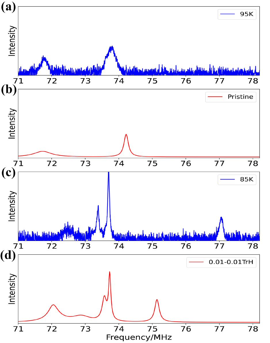
Figure S1: The NQR spectra for experimental results and manually adjusted 0.01-0.01 TrH. (a) The experimental spectrum Mu et al. (2022) at 95K (above $T_{s}$). (b) The calculated spectrum of the pristine structure. (c) The experimental spectrum Mu et al. (2022) at 85K (below $T_{s}$). (d) The calculated spectrum of the 0.01-0.01 TrH structure. For comparison purposes, the calculated results are shifted by +5.75MHz.

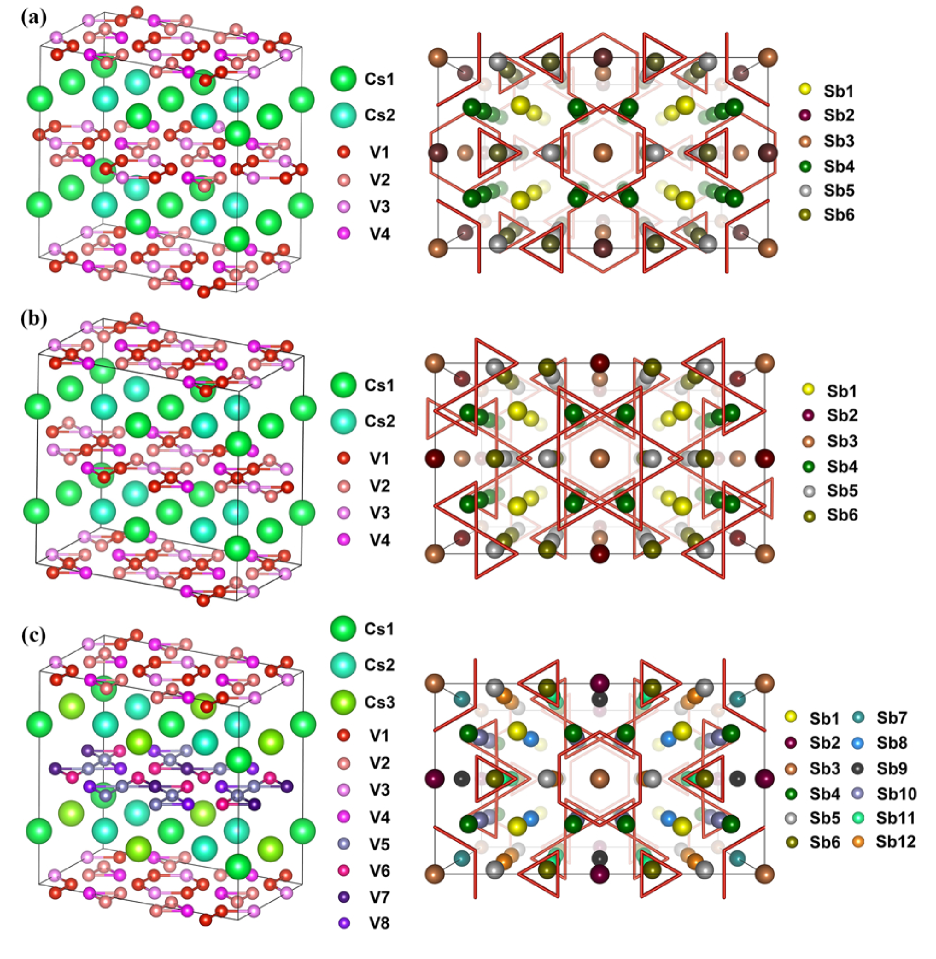
Figure S2: The different kinds of non-equivalent atoms of CsV3Sb5.(a)$2a\times 2a\times 2c$ pure TrH.(b)$2a\times 2a\times 2c$ pure SoD.(c)$2a\times 2a\times 2c$ mixed structure.The left half of the graph contains only Cs atoms and V atoms, and the right half of the graph contains only Sb atoms and bonds between V atoms.

References

- Ortiz et al. (2019) Brenden R. Ortiz, Lídia C. Gomes, Jennifer R. Morey, Michal Winiarski, Mitchell Bordelon, John S. Mangum, Iain W. H. Oswald, Jose A. Rodriguez-Rivera, James R. Neilson, Stephen D. Wilson, Elif Ertekin, Tyrel M. McQueen, and Eric S. Toberer, “New kagome prototype materials: discovery of \ceKV3Sb5,\ceRbV3Sb5, and \ceCsV3Sb5,” Phys. Rev. Materials 3, 094407 (2019).
- Ortiz et al. (2020) Brenden R. Ortiz, Samuel M. L. Teicher, Yong Hu, Julia L. Zuo, Paul M. Sarte, Emily C. Schueller, A. M. Milinda Abeykoon, Matthew J. Krogstad, Stephan Rosenkranz, Raymond Osborn, Ram Seshadri, Leon Balents, Junfeng He, and Stephen D. Wilson, “\ceCsV3Sb5: A topological kagome metal with a superconducting ground state,” Phys. Rev. Lett. 125, 247002 (2020).
- Ortiz et al. (2021a) Brenden R. Ortiz, Paul M. Sarte, Eric M. Kenney, Michael J. Graf, Samuel M. L. Teicher, Ram Seshadri, and Stephen D. Wilson, “Superconductivity in the kagome metal \ceKV3Sb5,” Phys. Rev. Materials 5, 034801 (2021a).
- Yin et al. (2021) Qiangwei Yin, Zhijun Tu, Chunsheng Gong, Yang Fu, Shaohua Yan, and Hechang Lei, “Superconductivity and Normal-State Properties of Kagome Metal \ceRbV3Sb5 Single Crystals,” Chinese Physics Letters 38, 037403 (2021), arXiv:2101.10193 [cond-mat.supr-con] .
- Liang et al. (2021) Zuowei Liang, Xingyuan Hou, Fan Zhang, Wanru Ma, Ping Wu, Zongyuan Zhang, Fanghang Yu, J.-J. Ying, Kun Jiang, Lei Shan, Zhenyu Wang, and X.-H. Chen, “Three-dimensional charge density wave and surface-dependent vortex-core states in a kagome superconductor \ceCsV3Sb5,” Phys. Rev. X 11, 031026 (2021).
- Chen et al. (2021) Hui Chen, Haitao Yang, Bin Hu, Zhen Zhao, Jie Yuan, Yuqing Xing, Guojian Qian, Zihao Huang, Geng Li, Yuhan Ye, Sheng Ma, Shunli Ni, Hua Zhang, Qiangwei Yin, Chunsheng Gong, Zhijun Tu, Hechang Lei, Hengxin Tan, Sen Zhou, Chengmin Shen, Xiaoli Dong, Binghai Yan, Ziqiang Wang, and Hong-Jun Gao, “Roton pair density wave in a strong-coupling kagome superconductor,” Nature 599, 222–228 (2021).
- Jiang et al. (2021) Kun Jiang, Tao Wu, Jia-Xin Yin, Zhenyu Wang, M. Zahid Hasan, Stephen D. Wilson, Xianhui Chen, and Jiangping Hu, “Kagome superconductors \ceAV3Sb5 (A=K, Rb, Cs),” arXiv e-prints , arXiv:2109.10809 (2021), arXiv:2109.10809 [cond-mat.supr-con] .
- Nie et al. (2022) Linpeng Nie, Kuanglv Sun, Wanru Ma, Dianwu Song, Lixuan Zheng, Zuowei Liang, Ping Wu, Fanghang Yu, Jian Li, Min Shan, Dan Zhao, Shunjiao Li, Baolei Kang, Zhimian Wu, Yanbing Zhou, Kai Liu, Ziji Xiang, Jianjun Ying, Zhenyu Wang, Tao Wu, and Xianhui Chen, “Charge-density-wave-driven electronic nematicity in a kagome superconductor,” Nature 604, 59–64 (2022).
- Mielke et al. (2022) C. Mielke, D. Das, J. X. Yin, H. Liu, R. Gupta, Y. X. Jiang, M. Medarde, X. Wu, H. C. Lei, J. Chang, Pengcheng Dai, Q. Si, H. Miao, R. Thomale, T. Neupert, Y. Shi, R. Khasanov, M. Z. Hasan, H. Luetkens, and Z. Guguchia, “Time-reversal symmetry-breaking charge order in a kagome superconductor,” Nature 602, 245–250 (2022).
- Jiang et al. (2021) Yu-Xiao Jiang, Jia-Xin Yin, M. Michael Denner, Nana Shumiya, Brenden R. Ortiz, Gang Xu, Zurab Guguchia, Junyi He, Md Shafayat Hossain, Xiaoxiong Liu, Jacob Ruff, Linus Kautzsch, Songtian S. Zhang, Guoqing Chang, Ilya Belopolski, Qi Zhang, Tyler A. Cochran, Daniel Multer, Maksim Litskevich, Zi-Jia Cheng, Xian P. Yang, Ziqiang Wang, Ronny Thomale, Titus Neupert, Stephen D. Wilson, and M. Zahid Hasan, “Unconventional chiral charge order in kagome superconductor \ceKV3Sb5,” Nature Materials 20, 1353–1357 (2021).
- Yu et al. (2021) Li Yu, Chennan Wang, Yuhang Zhang, Mathias Sander, Shunli Ni, Zouyouwei Lu, Sheng Ma, Zhengguo Wang, Zhen Zhao, Hui Chen, Kun Jiang, Yan Zhang, Haitao Yang, Fang Zhou, Xiaoli Dong, Steven L. Johnson, Michael J. Graf, Jiangping Hu, Hong-Jun Gao, and Zhongxian Zhao, “Evidence of a hidden flux phase in the topological kagome metal \ceCsV3Sb5,” arXiv e-prints , arXiv:2107.10714 (2021), arXiv:2107.10714 [cond-mat.supr-con] .
- Yu et al. (2021) F. H. Yu, T. Wu, Z. Y. Wang, B. Lei, W. Z. Zhuo, J. J. Ying, and X. H. Chen, “Concurrence of anomalous hall effect and charge density wave in a superconducting topological kagome metal,” Phys. Rev. B 104, L041103 (2021).
- Yang et al. (2020) Shuo-Ying Yang, Yaojia Wang, Brenden R. Ortiz, Defa Liu, Jacob Gayles, Elena Derunova, Rafael Gonzalez-Hernandez, Libor Šmejkal, Yulin Chen, Stuart S. P. Parkin, Stephen D. Wilson, Eric S. Toberer, Tyrel McQueen, and Mazhar N. Ali, “Giant, unconventional anomalous hall effect in the metallic frustrated magnet candidate, \ceKV3Sb5,” Science Advances 6, eabb6003 (2020), https://www.science.org/doi/pdf/10.1126/sciadv.abb6003 .
- Zhou et al. (2022) Xuebo Zhou, Hongxiong Liu, Wei Wu, Kun Jiang, Youguo Shi, Zheng Li, Yu Sui, Jiangping Hu, and Jianlin Luo, “Anomalous thermal hall effect and anomalous nernst effect of \ceCsV3Sb5,” Phys. Rev. B 105, 205104 (2022).
- Feng et al. (2021) Xilin Feng, Kun Jiang, Ziqiang Wang, and Jiangping Hu, “Chiral flux phase in the kagome superconductor \ceAV3Sb5,” Science Bulletin 66, 1384–1388 (2021).
- Wu et al. (2021) Qiong Wu, Z. X. Wang, Q. M. Liu, R. S. Li, S. X. Xu, Q. W. Yin, C. S. Gong, Z. J. Tu, H. C. Lei, T. Dong, and N. L. Wang, “Revealing the immediate formation of two-fold rotation symmetry in charge-density-wave state of Kagome superconductor \ceCsV3Sb5 by optical polarization rotation measurement,” arXiv e-prints , arXiv:2110.11306 (2021), arXiv:2110.11306 [cond-mat.supr-con] .
- Xu et al. (2022) Yishuai Xu, Zhuoliang Ni, Yizhou Liu, Brenden R. Ortiz, Stephen D. Wilson, Binghai Yan, Leon Balents, and Liang Wu, “Universal three-state nematicity and magneto-optical Kerr effect in the charge density waves in \ceAV3Sb5 (A=Cs, Rb, K),” arXiv e-prints , arXiv:2204.10116 (2022), arXiv:2204.10116 [cond-mat.str-el] .
- Park et al. (2021) Takamori Park, Mengxing Ye, and Leon Balents, “Electronic instabilities of kagome metals: Saddle points and landau theory,” Phys. Rev. B 104, 035142 (2021).
- Denner et al. (2021) M. Michael Denner, Ronny Thomale, and Titus Neupert, “Analysis of charge order in the kagome metal \ceAV3Sb5 (A=\ceK, \ceRb, \ceCs),” Phys. Rev. Lett. 127, 217601 (2021).
- Lin and Nandkishore (2021) Yu-Ping Lin and Rahul M. Nandkishore, “Complex charge density waves at van hove singularity on hexagonal lattices: Haldane-model phase diagram and potential realization in the kagome metals \ceAV3Sb5 (A=\ceK, \ceRb, \ceCs),” Phys. Rev. B 104, 045122 (2021).
- Li et al. (2021) Haoxiang Li, T. T. Zhang, T. Yilmaz, Y. Y. Pai, C. E. Marvinney, A. Said, Q. W. Yin, C. S. Gong, Z. J. Tu, E. Vescovo, C. S. Nelson, R. G. Moore, S. Murakami, H. C. Lei, H. N. Lee, B. J. Lawrie, and H. Miao, “Observation of unconventional charge density wave without acoustic phonon anomaly in kagome superconductors \ceAV3Sb5 (A=\ceRb, \ceCs),” Phys. Rev. X 11, 031050 (2021).
- Miao et al. (2021) H. Miao, H. X. Li, W. R. Meier, A. Huon, H. N. Lee, A. Said, H. C. Lei, B. R. Ortiz, S. D. Wilson, J. X. Yin, M. Z. Hasan, Ziqiang Wang, Hengxin Tan, and Binghai Yan, “Geometry of the charge density wave in the kagome metal \ceAV3Sb5,” Phys. Rev. B 104, 195132 (2021), arXiv:2106.10150 [cond-mat.str-el] .
- Ortiz et al. (2021b) Brenden R. Ortiz, Samuel M. L. Teicher, Linus Kautzsch, Paul M. Sarte, Noah Ratcliff, John Harter, Jacob P. C. Ruff, Ram Seshadri, and Stephen D. Wilson, “Fermi surface mapping and the nature of charge-density-wave order in the kagome superconductor \ceCsV3Sb5,” Phys. Rev. X 11, 041030 (2021b).
- Kautzsch et al. (2023) Linus Kautzsch, Brenden R. Ortiz, Krishnanand Mallayya, Jayden Plumb, Ganesh Pokharel, Jacob P. C. Ruff, Zahirul Islam, Eun-Ah Kim, Ram Seshadri, and Stephen D. Wilson, “Structural evolution of the kagome superconductors (A = K, Rb, and Cs) through charge density wave order,” Phys. Rev. Mater. 7, 024806 (2023).
- Mu et al. (2021) Chao Mu, Qiangwei Yin, Zhijun Tu, Chunsheng Gong, Hechang Lei, Zheng Li, and Jianlin Luo, “S-wave superconductivity in kagome metal \ceCsV3Sb5 revealed by \ce^121/123Sb NQR and \ce^51V NMR measurements,” Chinese Physics Letters 38, 077402 (2021).
- Song et al. (2022) DianWu Song, LiXuan Zheng, FangHang Yu, Jian Li, LinPeng Nie, Min Shan, Dan Zhao, ShunJiao Li, BaoLei Kang, ZhiMian Wu, YanBing Zhou, KuangLv Sun, Kai Liu, XiGang Luo, ZhenYu Wang, JianJun Ying, XianGang Wan, Tao Wu, and XianHui Chen, “Orbital ordering and fluctuations in a kagome superconductor \ceCsV3Sb5,” Science China Physics, Mechanics & Astronomy 65, 247462 (2022).
- Mu et al. (2022) Chao Mu, Qiangwei Yin, Zhijun Tu, Chunsheng Gong, Ping Zheng, Hechang Lei, Zheng Li, and Jianlin Luo, “Tri-hexagonal charge order in kagome metal \ceCsV3Sb5 revealed by \ce^121Sb nuclear quadrupole resonance,” Chinese Physics B 31, 017105 (2022).
- Luo et al. (2022a) J. Luo, Z. Zhao, Y. Z. Zhou, J. Yang, A. F. Fang, H. T. Yang, H. J. Gao, R. Zhou, and Guo-qing Zheng, “Possible star-of-david pattern charge density wave with additional modulation in the kagome superconductor \ceCsV3Sb5,” npj Quantum Materials 7, 30 (2022a).
- Zhao et al. (2021) He Zhao, Hong Li, Brenden R. Ortiz, Samuel M. L. Teicher, Takamori Park, Mengxing Ye, Ziqiang Wang, Leon Balents, Stephen D. Wilson, and Ilija Zeljkovic, “Cascade of correlated electron states in the kagome superconductor \ceCsV3Sb5,” Nature 599, 216–221 (2021).
- Luo et al. (2022b) Hailan Luo, Qiang Gao, Hongxiong Liu, Yuhao Gu, Dingsong Wu, Changjiang Yi, Junjie Jia, Shilong Wu, Xiangyu Luo, Yu Xu, Lin Zhao, Qingyan Wang, Hanqing Mao, Guodong Liu, Zhihai Zhu, Youguo Shi, Kun Jiang, Jiangping Hu, Zuyan Xu, and X. J. Zhou, “Electronic nature of charge density wave and electron-phonon coupling in kagome superconductor \ceKV3Sb5,” Nature Communications 13, 273 (2022b).
- Tan et al. (2021) Hengxin Tan, Yizhou Liu, Ziqiang Wang, and Binghai Yan, “Charge density waves and electronic properties of superconducting kagome metals,” Phys. Rev. Lett. 127, 046401 (2021).
- Christensen et al. (2021) Morten H. Christensen, Turan Birol, Brian M. Andersen, and Rafael M. Fernandes, “Theory of the charge density wave in kagome metals,” Phys. Rev. B 104, 214513 (2021).
- Ptok et al. (2022) Andrzej Ptok, Aksel Kobiałka, Małgorzata Sternik, Jan Łażewski, Paweł T. Jochym, Andrzej M. Oleś, and Przemysław Piekarz, “Dynamical study of the origin of the charge density wave in (, Rb, Cs) compounds,” Phys. Rev. B 105, 235134 (2022).
- Suits (2006) Bryan H. Suits, “Nuclear quadrupole resonance spectroscopy,” in Handbook of Applied Solid State Spectroscopy, edited by D. R. Vij (Springer US, Boston, MA, 2006) pp. 65–96.
- Slichter (1996) Charles P Slichter, Principles of Magnetic Resonance, Vol. 1 (Springer Science & Business Media, 1996).
- Martin (2020) Richard M Martin, Electronic structure: basic theory and practical methods (Cambridge university press, 2020).
- Singh and Nordstrom (2006) David J Singh and Lars Nordstrom, Planewaves, Pseudopotentials, and the LAPW method (Springer Science & Business Media, 2006).
- Sjöstedt et al. (2000) Elisabeth Sjöstedt, Lars Nordström, and DJ Singh, “An alternative way of linearizing the augmented plane-wave method,” Solid state communications 114, 15–20 (2000).
- Blaha et al. (2020) Peter Blaha, Karlheinz Schwarz, Fabien Tran, Robert Laskowski, Georg KH Madsen, and Laurence D Marks, “WIEN2k: An APW+lo program for calculating the properties of solids,” The Journal of Chemical Physics 152, 074101 (2020).
- Schwarz et al. (2010) Karlheinz Schwarz, Peter Blaha, and SB Trickey, “Electronic structure of solids with WIEN2k,” Molecular Physics 108, 3147–3166 (2010).
- Laskowski and Blaha (2015) Robert Laskowski and Peter Blaha, “NMR shielding in metals using the augmented plane wave method,” The Journal of Physical Chemistry C 119, 19390–19396 (2015).
- Ebert et al. (1986) H Ebert, H Winter, and J Voitlander, “A real-space formulation for the spin and orbital contributions to the knight shift in metallic systems: application to \ceV, \ceCr, \ceNb and \ceMo,” Journal of Physics F: Metal Physics 16, 1133 (1986).
- Wu et al. (2022) Shangfei Wu, Brenden R. Ortiz, Hengxin Tan, Stephen D. Wilson, Binghai Yan, Turan Birol, and Girsh Blumberg, “Charge density wave order in the kagome metal ,” Phys. Rev. B 105, 155106 (2022).
- Xiao et al. (2022) Qian Xiao, Yihao Lin, Qizhi Li, Wei Xia, Xiquan Zheng, Shilong Zhang, Yanfeng Guo, Ji Feng, and Yingying Peng, “Coexistence of Multiple Stacking Charge Density Waves in Kagome Superconductor ,” arXiv e-prints , arXiv:2201.05211 (2022), arXiv:2201.05211 [cond-mat.supr-con] .
- Frassineti et al. (2022) Jonathan Frassineti, Pietro Bonfà, Giuseppe Allodi, Erick Garcia, Rong Cong, Brenden R. Ortiz, Stephen D. Wilson, Roberto De Renzi, Vesna F. Mitrović, and Samuele Sanna, “Microscopic nature of the charge-density wave in kagome superconductor RbV3Sb5,” arXiv preprint arXiv:2210.06523 (2022).
- Laskowski and Blaha (2012) Robert Laskowski and Peter Blaha, “Calculations of NMR chemical shifts with APW-based methods,” Physical Review B 85, 035132 (2012).
- Baroni et al. (2001) Stefano Baroni, Stefano De Gironcoli, Andrea Dal Corso, and Paolo Giannozzi, “Phonons and related crystal properties from density-functional perturbation theory,” Reviews of modern Physics 73, 515 (2001).
- Novak (2006) P Novak, “Calculation of hyperfine field in WIEN2k,” energy 2, 9 (2006).
- Blügel et al. (1987) S Blügel, H Akai, R Zeller, and PH Dederichs, “Hyperfine fields of 3d and 4d impurities in nickel,” Physical Review B 35, 3271 (1987).
- Laskowski et al. (2017) Robert Laskowski, Khoong Hong Khoo, Frank Haarmann, and Peter Blaha, “Computational study of Ga NMR shielding in metallic gallides,” The Journal of Physical Chemistry C 121, 753–760 (2017).
- Abragam and Bleaney (2012) Anatole Abragam and Brebis Bleaney, Electron paramagnetic resonance of transition ions (Oxford University Press, 2012).