Deep PatchMatch MVS with Learned Patch Coplanarity, Geometric Consistency and Adaptive Pixel Sampling

Abstract

Recent work in multi-view stereo (MVS) combines learnable photometric scores and regularization with PatchMatch-based optimization to achieve robust pixelwise estimates of depth, normals, and visibility. However, non-learning based methods still outperform for large scenes with sparse views, in part due to use of geometric consistency constraints and ability to optimize over many views at high resolution. In this paper, we build on learning-based approaches to improve photometric scores by learning patch coplanarity and encourage geometric consistency by learning a scaled photometric cost that can be combined with reprojection error. We also propose an adaptive pixel sampling strategy for candidate propagation that reduces memory to enable training on larger resolution with more views and a larger encoder. These modifications lead to 6-15% gains in accuracy and completeness on the challenging ETH3D benchmark, resulting in higher $F_{1}$ performance than the widely used state-of-the-art non-learning approaches ACMM and ACMP.

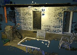
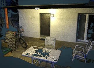
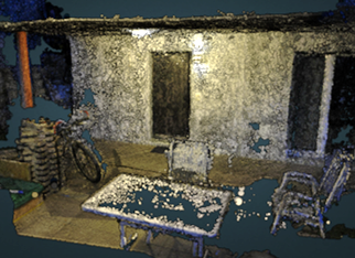
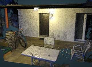
COLMAP schoenberger2016mvs	ACMM xu2019multi	PatchMatch-RL lee2021patchmatchrl	Ours

Figure 1: We propose a learning-based PatchMatch MVS approach with learned patch coplanarity, geometric consistency and adaptive pixel sampling. Our method achieves more complete reconstruction compared to existing MVS methods.

1 Introduction

Multi-view stereo (MVS) aims to infer accurate and complete 3D geometry from a set of calibrated images, with many applications such as robotics furukawa2009accurate ; rebecq2018emvs , mixed reality yang2013image ; prokopetc2019towards , and vision-based inspection golparvar2011monitoring . The first deep learning-based approaches work well for densely sampled views with small-scaled scenes, such as the DTU dataset aanaes2016large and the Tanks-and-Temples intermediate benchmark Knapitsch2017tanks . However, in more challenging benchmarks with sparse views, wide baselines, and large depth ranges, such as the ETH3D High-res benchmark schoeps2017eth3d , non-learning based methods achieve better performance by jointly optimizing over many views for the depths, normals, and visibilities of each pixel that maximize photometric scores while satisfying geometric consistency. Recent methods incorporate PatchMatch optimization into an end-to-end training framework wang2020patchmatchnet ; lee2021patchmatchrl , partially closing the performance gap. The latest work PatchMatch-RL lee2021patchmatchrl proposes to jointly learn from pixel-wise depth, normal, and visibility, by using reinforcement learning to overcome the non-differentiable PatchMatch optimization. However, methods such as ACMM xu2019multi still outperform, in part due to the precision of the bilaterally weighted NCC photometric cost, the ability to optimize over many views at high resolution, and the ability to incorporate geometric consistency constraints.

In this paper, we propose three designs to address the above-mentioned issues of learning-based PatchMatch MVS. First, we improve the photometric cost function by directly learning whether nearby pixels are co-planar. Patch-based MVS methods compute photometric score by comparing intensities or features over some neighborhood after rectifying for depth and normal, under the assumption that the surface is locally planar. Existing approaches weight the neighborhood based on color and pixel distance schoenberger2016mvs or dot-product attention between feature vectors lee2021patchmatchrl . We modify the affinity neighborhood network CSPN cheng2019learning to directly learn which neighboring points are likely coplanar, which provides weights for more robust photometric costs in both textureless and textured regions.

Second, we incorporate geometric consistency regularization, replacing the recurrent cost regularization of PatchMatch-RL lee2021patchmatchrl . Although geometric consistency is commonly used in non-learning approaches (e.g., schoenberger2016mvs ; xu2019multi ; Xu2020ACMP ), integration in deep learning approaches is challenging, since the neighborhood geometry is not differentiable with respect to the reference view geometry. We side-step this problem by learning to map the photometric score into a log-disbelief (i.e., negative log likelihood) and model reprojection error with a Gaussian distribution, such that the joint likelihood is the sum of photometric log-disbelief and the L2-norm reprojection error.

Finally, we investigate how to train learning-based PatchMatch MVS to perform inference with high-resolution images, more views, and deeper features. The challenge is that higher resolutions require larger receptive fields to include sufficiently discriminate texture. Coarse-to-fine architectures xu2019multi ; wang2020patchmatchnet ; lee2021patchmatchrl help, but more complex features with larger receptive fields are also required, which in turn requires prohibitive quantities of GPU memory. We propose adaptive sampling of the supporting pixels and gradient checkpointing to reduce the memory usage in the training. This enables more PatchMatch iterations and larger sets of view selections and source views during training, as well as use of a U-Net ronneberger2015u -shaped feature extractor that covers a much larger receptive field compared to the shallow VGG-style backbone used in lee2021patchmatchrl .

In summary, our main contributions are:

• Learned coplanarity which weights the photometric score support based on estimated coplanarity.

• Modeling geometry consistency guided inference with learned photometric score functions which improves completion of the reconstruction.

• Efficient training using adaptively sampled subset of supporting pixels that reduces memory usage in the training time to allow: a) more PatchMatch training iterations, b) a larger set of source images, c) a larger number of pixel-wise view selections and d) a more complex feature extraction backbone.

Combined, our method outperforms state-of-the-art learning-based MVS methods on the ETH3D high-res benchmark by a large margin with the same image resolution. We also provide an efficient and scalable inference architecture that enables high-resolution inference on up to 10 source images of $3200\times 2112$, outperforming the classical counterpart methods ACMM xu2019multi and ACMP Xu2020ACMP at the same image resolution.

2 Related Works

The goal of multi-view stereo (MVS) is to estimate the scene geometry using the images with the known poses. We refer readers to Furukawa and Hernández furukawa2015_mvsTutorial for a broad review and focus on the most related work here.

Stereo based depth estimation methods hypothesize depth values and score the hypotheses based on photometric similarity (or matching cost). Initial works lucasKanade1981_stereo ; hannah1974computer ; anandan1989computational compute the matching cost as the sum of square differences or absolute differences between corresponding pixels in a local patch. This simple score is unreliable for oblique surfaces, near depth discontinuities, and for low-texture or non-Lambertian surfaces. MVS approaches evolved to address these concerns by jointly estimating depth and normal for each pixel bleyer2011patchmatch , assigning weights to supporting pixels schoenberger2016mvs , and using robust matching functions, e.g. learned or NCC, as well as regularizing the cost based on neighborhood estimates or scores yao2018mvsnet ; yao2019recurrent ; gu2020cascade ; luo2020attention . The joint depth and normal search has been implemented by using PatchMatch barnes2009patchmatch based optimization by Bleyer et al. bleyer2011patchmatch , and extended to multi-view stereo with visibility selection zheng2014patchmatch ; galliani2015massively ; schoenberger2016mvs . Incorporation of normal estimates enables a more accurate patch-wise homography to match views of oblique surfaces, but depth discontinuities remain a problem. To address depth discontinuities, bilaterally weighted normalized cross correlation (NCC) is proposed schoenberger2016mvs , with weights modeling the likelihood of the coplanarity of each supporting pixel as proportional to a product of color and position difference terms. Bilaterally weighted NCC is widely used in recent non-learning PatchMatch-based methods xu2019multi ; romanoni2019tapa ; Xu2020ACMP ; kuhn2020deepc ; wang2020mesh ; xu2020marmvs .

In learning-based PatchMatch MVS, Lee et al. lee2021patchmatchrl use scaled dot-product based attention to model supporting pixel weights. Both bilaterally weighted NCC and scaled dot-product attention rely on center-pixel similarity to measure the local co-planarity of the supporting pixels. However, when pixels across depth boundaries have similar colors or flat surfaces have varying texture, center-pixel similarity does not correctly model coplanarity. Instead, we propose to directly regress the supporting pixel-wise co-planarity using ground-truth supervision.

Local photometric scores are unpredictive or unreliable for textureless or non-Lambertian surfaces, requiring consistency checks across neighborhoods or other views. COLMAP schoenberger2016mvs checks the consistency of predicted depths and normals with neighboring views to augment the photometric score and filter inconsistent points, improving accuracy but decreasing recall. ACMM xu2019multi propose a coarse-to-fine geometric consistency regularized inference. Reconstruction at coarse resolutions enables photometric scores with wide receptive fields with more texture, yielding more accurate but imprecise depth estimates, that are then refined at finer scales using a combination of geometric consistency and photometric cost terms. Our work combines the coarse-to-fine geometric consistency driven inference with the learning based PatchMatch MVS by mapping the learned photometric score into a log-disbelief scale, which allows the optional aggregation of additional log-disbelief terms, such as a geometric consistency term.

DeepC-MVS kuhn2020deepc achieves state-of-the-art results on ETH3D by adding a post-process refinement step to a slightly modified version of ACMM, filtering or refining depth values using learned confidences based on the initial estimates of depth, normal, and visibility. Similar refinements would likely benefit learning-based approaches also, but we leave this to future work.

The state-of-the-art learning-based methods, Vis-MVSNet zhang2020visibility and EPP-MVSNet ma2021eppmvsnet operate on high-resolution images, which allows more definite reconstruction as pixel-level precision improves as frustums corresponding to each projection pixels become narrower. Both Vis-MVSNet zhang2020visibility and EPP-MVSNet ma2021eppmvsnet use U-Net ronneberger2015u as a shared CNN based encoder, which is known to preserve high-frequency details and provide wider receptive fields that make the encoder more suitable for high-resolution reconstruction.

We additionally integrate the learned patch coplanarity to sample the subset of supporting pixels in training time. This allows time and memory efficient training using policy gradient lee2021patchmatchrl , which lets our method to be trained with more PatchMatch iterations and source view selections per pixel, as well as using 2D U-Net ronneberger2015u based feature extraction.

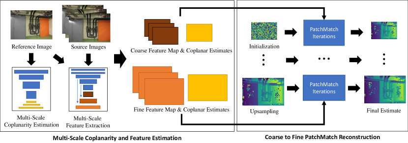
Figure 2: Training Architecture overview: We extract multiscale features for each image and multiscale coplanarity weights for the reference image. We use features and coplanar maps of corresponding scales to perform coarse-to-fine estimation of depth, normal and visibility maps. At the coarsest stage, we initialize pixelwise depth and normal maps. Then, a series of PatchMatch iterations update the estimates. The PatchMatch iteration consists of four stages: (1) pixelwise view selection; (2) candidate propagation; (3) candidate scoring; and (4) candidate selection. The current solution is then upsampled to a finer level of input through nearest neighbor interpolation, and this procedure continues until the oriented point estimates at the finest level are fused from all images.

3 Method

Figure 2 shows an overview of our architecture during training. We build our approach on PatchMatch-RL (Sec. 3.1), a recent learning-based PatchMatch MVS framework, and propose three designs that lead to large performance gain in both accuracy and completeness: (1) improve the photometric cost function by directly modeling the coplanarity of neighboring pixels (Sec. 3.2); (2) replace the recurrent cost regularization with geometric consistency by learning a scaled photometric cost  (Sec. 3.3); (3) design an adaptive pixel sampling strategy for candidate propagation to reduce memory, so that high-res images, more views, and deeper features can be used for training (Sec. 3.4).

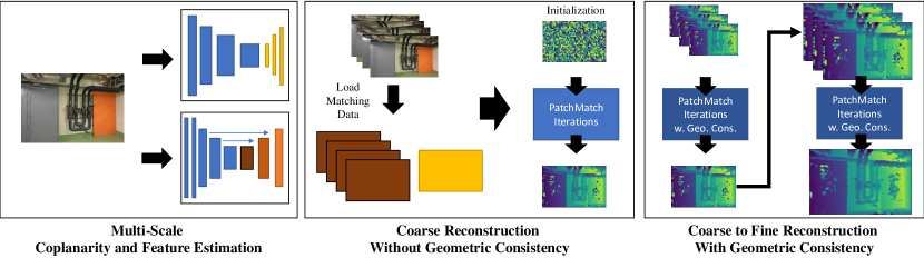
Figure 3: Inference Architecture: First, features and coplanar maps for each image are generated and stored in files. Then, coarse-level reconstruction without geometric consistency constraints is performed for each reference image. Specifically, the relevant coarse coplanar and feature maps are loaded and, after initializing depths and normals, a PatchMatch iteration (Figure 2) is performed to infer geometry. Next, coarse-to-fine reconstruction is performed with geometric consistency. For each stage, results from the previous stage are used to initialize estimates and compute geometric consistency scores. All images in the scene are processed stagewise, and the inference is complete once the finest scale is processed.

3.1 Review of PatchMatch-RL

The input of PatchMatch-RL is a set of reference and source images $\{I_{r},I_{i}\}^{N}_{i=1}\subset\mathcal{I}$, and their corresponding cameras poses $\{C_{r},C_{i}=(K_{i},R_{i},t_{i})\}^{N}_{i=1}\subset\mathcal{C}$ including intrinsic and extrinsic parameters. The method uses a coarse-to-fine PatchMatch MVS inference to jointly estimate the depths, normals, and visiblities of the reference image $D_{r},N_{r},\{V_{r,i}\}^{N}_{i=1}$, and uses policy-gradient for end-to-end training.

PatchMatch-RL starts by extracting CNN based features $\{f^{c}_{\theta}(I_{r})=F^{s}_{r},f^{c}_{\theta}(I_{i})=F^{s}_{i}\}^{N}_{i=1}$ at multiple scales $s\in\{3,2,1\}$, where $f^{c}_{\theta}$ represents trainable CNN backbone with parameters $\theta$, and $s$ represents the $\log_{2}$ scale resolution of the image (e.g. $F^{s}_{i}\rightarrow\mathbb{R}^{\frac{H}{2^{s}}\times\frac{W}{2^{s}}\times C}$). Then, the method initializes the depth and normal map $d^{s,t}_{r},n^{s,t}_{r}$ at the coarsest scale $s=3$ and the initial iteration $t=0$. For the ease of notation, we drop the scale $s$ and let $d^{t}_{r},n^{t}_{r},v^{t}_{r,i}$ denote the depth, normal and visibility map at the $t$-th iteration on the same scale in the coarse-to-fine stage from onward.

After initialization, a series of PatchMatch iterations are run at each scale, and each iteration jointly updates the depth, normal, and visibility maps. A single PatchMatch iteration consists of 4 steps:

1. Pixel-wise view selection updates the visiblity map $v^{t}_{r,i}\rightarrow v^{t+1}_{r,i}$ using the current set of depth $d^{t}_{r}$ and normal $n^{t}_{r}$ scored by an MLP $f^{v}_{\theta}$, which defines the parameterized view-sampling policy $\pi^{v}_{\theta}$.

2. Candidate Propagation generates potential candidates of depth and normal for the next iteration by using PatchMatch-based propagation.

3. Candidate Scoring scores each candidate depth / normal pairs using the current set of visibility map $v^{t+1}_{r,i}$ through an RNN-based scorer regularizer $f^{s}_{\theta}$, which defines the parameterized candidate-sampling policy $\pi^{s}_{\theta}$.

4. Candidate Selection updates the current depth and normal map to $d^{t+1}_{r}$ and $n^{t+1}_{r}$,

The parameterized policies represents the sampling procedure defined by the distribution formed by the scores obtained by the MLP $f^{v}_{\theta}$ and the RNN $f^{s}_{\theta}$. The view selection score distribution takes the supporting pixel-aggregated group-wise correlation scores for each source images as input. The supporting pixel-aggregated group-wise correlation scores use supporting pixel weights, obtained by the dot-product attention between the features at the center pixel and the supporting pixels, to compute weighted mean of the group-wise correlation scores between the pixels of reference feature map and the corresponding pixels of the source feature map. Given supporting pixels $q\in W(p)$ around the pixel $p$ and its corresponding weights $w(q)$, the supporting pixel-aggregated group-wise correlation of the pixel $p$ can be defined as:

$$\mathcal{G}(p)=\sum_{s=1}^{N}\sum_{q\in W(p)}w(q)(F^{r}(q)\circledast F^{s}(q^{\prime}))/N$$ (1)

where $q^{\prime}$ indicates the corresponding pixel of $q$ in the source image warped by the depth $d_{r}(p)$ and normal $n_{r}(p)$ value at $p$.

Similarly, the candidate scoring distribution obtained through $f^{s}_{\theta}$, takes view-weighted, supporting pixel aggregated group-wise correlation scores for selected views as input:

$$\mathcal{G}^{\mathcal{V}}_{\phi}(p)=\sum_{s\in\mathcal{V}}\sum_{q\in W(p)}v_{r,s}(p)w(q)(F^{r}(q)\circledast F^{s}(q^{\phi}))$$ (2)

where $\mathcal{V}$ is the set of selected views, and $v_{r,s}(p)$ indicates visibility estimate of the pixel $p$ in the reference image $r$ from the source image $s$, and $q^{\phi}$ denotes the corresponding pixel of $q$ in the source image, warped by the candidate depth $d_{\phi}(p)$ and normal $n_{\phi}(p)$. The output value of the RNN $f^{s}_{\theta}$ measures the photometric score of each candidate as $S^{\phi}_{pho}(p)=f^{s}_{\theta}(\mathcal{G}^{\mathcal{V}}_{\phi}(p))$.

In inference, the policy performs arg-max selection based on the set of computed scores. In training, the policy performs selection based on the decaying $\epsilon$-greedy method, where it samples from the distribution with the probability of $\epsilon$ and samples using arg-max with the probability of $1-\epsilon$.

After a sufficient number of iterations for each scale, the depth and normal maps are upscaled using nearest neighbor upsampling. Then, the next stage of the coarse-to-fine architecture starts, and the process is repeated until the most finest-level iteration is completed.

Figure 4: Coplanarity Extraction and Representation: We use a coplanar extractor to estimate the coplanar values of the supporting pixels of each pixel in the image. The output coplanarity map is an array of shape $H\times W\times 9$, where each position represents the corresponding $3\times 3$ supporting pixels of the image.

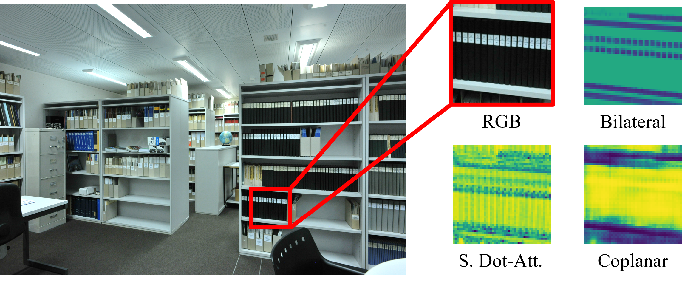
Figure 5: Comparison of Supporting Weights: We visualize different types of the supporting pixel weights that are 3 pixel above from the center. From the left top, RGB denotes the extracted patch for the reference, Bilateral denotes the bilateral weighting schoenberger2016mvs , S. Dot-Att. denotes scaled dot-product attention lee2021patchmatchrl and Coplanar denotes our learned coplanar weights. Our method more correctly identifies which pixels correspond to coplanar surfaces, e.g. tags on binders are coplanar with dark part of binders, while shelves are not.

To train the model in an end-to-end differentiable manner, PatchMatch-RL uses policy-gradient algorithm REINFORCE to jointly train $f^{c}_{\theta},f^{v}_{\theta},f^{s}_{\theta}$. The reward for each iteration is defined as $r^{t}=\mathcal{N}(d^{t}_{r}\mathchar 24635\relax\;D^{*}_{r},\sigma_{d})\cdot\mathcal{N}(n^{t}_{r}\mathchar 24635\relax\;N^{*}_{r},\sigma_{n})$, where $D^{*}_{r}$ and $N^{*}_{r}$ represent the ground-truth depth and normal maps, and $\mathcal{N}(x\mathchar 24635\relax\;\mu,\sigma)$ represents the probability of observing $x$ from the normal distribution with mean $\mu$ and standard deviation $\sigma$. The update for each iteration is:

$$\triangledown_{\theta}J =\sum_{t}\sum_{t^{\prime}>=t}\triangledown_{\theta}\gamma^{t^{\prime}-t}r^{t}\log\pi_{\theta}.$$ (3)

We let $\gamma$ represent the discount coefficient of future reward. PatchMatch-RL additionally modifies the candidate selection loss to use cross-entropy between the ground-truth distribution of observing each candidate (e.g. $\forall(d,n),\mathcal{N}(d\mathchar 24635\relax\;D^{*}_{r},\sigma_{d})\cdot\mathcal{N}(n\mathchar 24635\relax\;N^{*}_{r},\sigma_{n})$) and the distribution formed by the scores of each candidates using the candidate scoring policy for robustness in training.

3.2 Learning Patch Coplanarity

Estimating the surface normal for each pixel requires a patch-based photometric score, computed as a weighted sum of similarities over supporting interpolated feature positions. Rather than computing weights using scaled dot-product attention like PatchMatch-RL, we propose to set the weights to the likelihood of coplanarity with supporting pixels, which is estimated using a separate CNN architecture. (i.e., we directly estimate $w(q)$ for $q\in W(p)$ in Eqs. 1 and 2) We modify the CSPN architecture cheng2019learning used to learn the affinity of neighboring points, and change its last layer to a $3\times 3$ convolution with a dilation of 3, so that the receptive field matches the supporting pixel weight locations. Figure 4 depicts an overview of our coplanarity extraction and output feature representation. In addition to the policy gradient loss, we use mean squared error term from the ground-truth coplanarity points obtained from the ground-truth depth to supervise the the training. We show in Figure 5 that compared with existing supporting pixel weighting schemes, our approach can better identify coplanarity within local patches with different textures.

3.3 Encouraging Geometric Consistency in Inference

We propose geometric consistency based regularization to replace the recurrent cost regularization used in PatchMatch-RL. The key idea of geometric consistency is to use the inferred geometry of the source images to validate the reference image geometry. We adopt the geometric consistency score used in ACMM xu2019multi , which defines an additional score term based on the reprojection error of the visible source view pixels.

Although geometric consistency is commonly used for non-learning based approaches schoenberger2016mvs ; xu2019multi , it is challenging to integrate in learning-based approaches, since the source view geometry is not differentiable with respect to the reference view geometry. In order to allow the optional adding of geometric log-disbelief scores in candidate selection stage without having to train additional module to combine the two scores, we remap the photometric score and the geometric consistency score range to the log-disbelief range. In detail, we let the photometric score ranges logarithmically from $0$ to $S_{max}$, where $0$ implies perfect photometric match and $S_{max}$ implies complete disagreement. We use MLP as the photometric consistency scorer to replace the RNN-based scorer $f^{s}_{\theta}$, since the history of candidate selection cannot handle the additional geometric consistency term in inference.

We let the pixel-wise reprojection error distance be the log scale disbelief score of the geometric consistency term. Given the candidate depth and normal map $d_{\phi},n_{\phi}=\phi$, we use the homography between image $j$ and image $k$ at pixel $p$ defined as $H^{\phi}_{j\rightarrow k}(p)=K_{k}\cdot(R_{j\rightarrow k}-\frac{t_{j\rightarrow k}\cdot n^{T}_{\phi}(p)}{d_{\phi}(p)})\cdot K^{-1}_{j}$, and compute the reprojection error:

$$E^{\phi}_{s}(p)=\mbox{{}\rm\sf\leavevmode\hbox{}\hbox{}\/} H^\phi_{s \rightarrow r}(H^\phi_{r \rightarrow s}(p) \cdot p) - p \mbox{{}\rm\sf\leavevmode\hbox{}\hbox{}}_2 \end{equation} We define $G_{max}$ as the maximum log-disbelief term that can be added to geometric consistency, and combine the score weighted by the visibility mapping weights: \begin{equation}S^{\phi}_{geo}(p)=\sum^{N}_{i=1}v^{t}_{r,i}\cdot(S^{\phi}_{pho}(p)+\min(E^{\phi}_{i}(p),G_{max}))\end{equation} where $S^{\phi}_{pho}(p)$ denotes the photometric score obtained from the MLP. We then use $S^{\phi}_{geo}(p)$ to select candidate for the pixel $p$, updating the depth $d_{r}(p)$ and normal $n_{r}(p)$ at the corresponding iteration. \par Since we need to have the source view geometry available to use geometric consistency based regularization, we use a modified version of the coarse-to-fine architecture, as illustrated in Figure~{}\ref{fig:inference}. In inference, the source view and its inferred geometry in the previous stage are used to calculate $S^{\phi}_{geo}$ for the candidate selection step of each PatchMatch iteration. The inferred depth and normal maps at each stage are stored in a file, and loaded in the next stage of reconstruction with geometric consistency. \par\par\par\@@numbered@section{subsection}{toc}{Adaptive Supporting Pixel Sampling} Training the learning-based PatchMatch MVS model using policy gradient requires memory linear to the number of depth, normal and visibility map evaluations ({e}.{g}.\ number of PatchMatch iterations), since the history of gradients need to be stored. Hence, PatchMatch-RL~{}\cite[cite]{\@@bibref{Authors Phrase1YearPhrase2}{lee2021patchmatchrl}{\@@citephrase{(}}{\@@citephrase{)}}} uses a shallow VGG-style backbone, with a small number of PatchMatch iterations per scale. We resolve this problem by using a sampled subset of the supporting pixels in training, which effectively reduces the training computation by half and the memory by roughly 30\%, so that a larger feature extraction backbone can be used with faster training. We use the distribution of the coplanar values of the supporting pixels as a sampling distribution. We sample 3 points out of 8 supporting pixels, (excluding the center pixel of the $3\times 3$ local supporting pixels), which is the minimum number of points that supports estimates of surface normal orientation. The adaptive supporting pixel sampling can be used in the inference time for faster runtime, at the cost of a slight drop in reconstruction quality. Table~{}\ref{tab:ablation} and Table~{}\ref{tab:ablation_hr} in Section~{}\ref{sec:experiments} show the detailed analysis of the effect of adaptive supporting pixel sampling in inference. \begin{figure*}[t] \centering\begin{tabular}[]{@{}c@{}cc@{}cc@{}c@{}}\includegraphics[width=69.38078pt]{images/qualitative/eth3d/pipes_00000001_gt_i.png}&\includegraphics[width=69.38078pt]{images/qualitative/eth3d/pipes_00000001_gt_d_.png}&\includegraphics[width=69.38078pt]{images/qualitative/eth3d/pipes_00000001_orig_d_.png}&\includegraphics[width=69.38078pt]{images/qualitative/eth3d/pipes_00000001_orig_n.png}&\includegraphics[width=69.38078pt]{images/qualitative/eth3d/pipes_00000001_ours_d_.png}&\includegraphics[width=69.38078pt]{images/qualitative/eth3d/pipes_00000001_ours_n.png}\\ \includegraphics[width=69.38078pt]{images/qualitative/eth3d/relief_00000014_gt_i.png}&\includegraphics[width=69.38078pt]{images/qualitative/eth3d/relief_00000014_gt_d_.png}&\includegraphics[width=69.38078pt]{images/qualitative/eth3d/relief_00000014_orig_d_.png}&\includegraphics[width=69.38078pt]{images/qualitative/eth3d/relief_00000014_orig_n.png}&\includegraphics[width=69.38078pt]{images/qualitative/eth3d/relief_00000014_ours_d_.png}&\includegraphics[width=69.38078pt]{images/qualitative/eth3d/relief_00000014_ours_n.png}\\ \includegraphics[width=69.38078pt]{images/qualitative/eth3d/relief_2_00000027_gt_i.png}&\includegraphics[width=69.38078pt]{images/qualitative/eth3d/relief_2_00000027_gt_d_.png}&\includegraphics[width=69.38078pt]{images/qualitative/eth3d/relief_2_00000027_orig_d_.png}&\includegraphics[width=69.38078pt]{images/qualitative/eth3d/relief_2_00000027_orig_n.png}&\includegraphics[width=69.38078pt]{images/qualitative/eth3d/relief_2_00000027_ours_d_.png}&\includegraphics[width=69.38078pt]{images/qualitative/eth3d/relief_2_00000027_ours_n.png}\\ \includegraphics[width=69.38078pt]{images/qualitative/eth3d/terrains_00000039_gt_i.png}&\includegraphics[width=69.38078pt]{images/qualitative/eth3d/terrains_00000039_gt_d_.png}&\includegraphics[width=69.38078pt]{images/qualitative/eth3d/terrains_00000039_orig_d_.png}&\includegraphics[width=69.38078pt]{images/qualitative/eth3d/terrains_00000039_orig_n.png}&\includegraphics[width=69.38078pt]{images/qualitative/eth3d/terrains_00000039_ours_d_.png}&\includegraphics[width=69.38078pt]{images/qualitative/eth3d/terrains_00000039_ours_n.png}\\ Ref. Image&GT. Depth&\lx@intercol\hfil PatchMatch-RL~{}\cite[cite]{\@@bibref{Authors Phrase1YearPhrase2}{lee2021patchmatchrl}{\@@citephrase{(}}{\@@citephrase{)}}}\hfil\lx@intercol &\lx@intercol\hfil$\text{Ours}_{hr}$\hfil\lx@intercol \end{tabular} \@@toccaption{{\lx@tag[ ]{{6}}{ {Qualitative comparison against PatchMatch-RL on the ETH3D high-res multi-view benchmark training scenes.} We show from the left the reference image, the ground-truth depth, the depth and normal estimated by PatchMatch-RL, the depth and normal estimated by $\text{Ours}_{hr}$. All depth maps share the same color scale based on the ground-truth depth ranges. Our method can reconstruct more accurate points in thin structure regions, and have less noise in texture-less surfaces. }}}\@@caption{{\lx@tag[: ]{{Figure 6}}{ {Qualitative comparison against PatchMatch-RL on the ETH3D high-res multi-view benchmark training scenes.} We show from the left the reference image, the ground-truth depth, the depth and normal estimated by PatchMatch-RL, the depth and normal estimated by $\text{Ours}_{hr}$. All depth maps share the same color scale based on the ground-truth depth ranges. Our method can reconstruct more accurate points in thin structure regions, and have less noise in texture-less surfaces. }}} \@add@centering\end{figure*} \par\@@numbered@section{section}{toc}{Experiments} We evaluate our method on two standard MVS benchmarks, ETH3D High-res Multi-View benchmark~{}\cite[cite]{\@@bibref{Authors Phrase1YearPhrase2}{schoeps2017eth3d}{\@@citephrase{(}}{\@@citephrase{)}}} and Tanks-and-Temples(TnT)~{}\cite[cite]{\@@bibref{Authors Phrase1YearPhrase2}{Knapitsch2017tanks}{\@@citephrase{(}}{\@@citephrase{)}}} intermediate and advanced benchmark. \par\par\@@numbered@section{subsection}{toc}{Implementation Details} For all benchmarks, we use BlendedMVS~{}\cite[cite]{\@@bibref{Authors Phrase1YearPhrase2}{yao2020blendedmvs}{\@@citephrase{(}}{\@@citephrase{)}}} dataset for training. BlendedMVS is a large-scale MVS dataset that contains 113 indoor, outdoor and object-level scenes. We use 7 images ({i}.{e}., 1 reference image and 6 source images) with an input resolution of $768\times 576$, and an output resolution of $384\times 288$ for training. Among the 6 source images, we use 3 images sampled from the 10 best matching source images given by the global view selection provided by the dataset, and 3 images randomly selected from the remaining images in the scene. In training local view selection, we consider the three best views to be visible and the two worst views to be not visible. In inference, we select the three best source views for reconstruction. Regarding the number of PatchMatch iterations for each scale, we use $N^{3}_{iter},N^{2}_{iter},N^{1}_{iter}$ = $8,2,1$ in training, and $8,3,3$ in inference respectively. We finally fuse the estimated depth and normal maps using the fusion method of Galliani et al.~{}\cite[cite]{\@@bibref{Authors Phrase1YearPhrase2}{galliani2015massively}{\@@citephrase{(}}{\@@citephrase{)}}}, where we filter depths by the number of minimum consistent views containing relative depth error below 1\%, reprojection error less than 2px and normal angle difference less than 10$\degree$. We apply nearest neighbor upsampling with $5\times 5$ median filtering to upscale the depth map to the same resolution of the original image during fusion. We implemented our method in PyTorch and use RTX 3090 for training and evaluation. We use a customized CUDA kernel to accelerate the computation of supporting pixel-aggregated group-wise correlation in inference. These design choices are evaluated in our ablation study (Sec.~{}\ref{exp_ablations}, Table~{}\ref{tab:ablation_additional}). \par\begin{table*}[t] \centering\@@toccaption{{\lx@tag[ ]{{1}}{ {Results on the ETH3D high-res Multi-View benchmark train and test sets.} All methods do not train on any ETH3D data. Bold and underline denote the method with the highest and the second highest score for each setting, respectively. $\text{Ours}_{hr}$ method outperforms all other methods in both 2cm and 5cm criteria in train and test scenes except DeepC-MVS~{}\cite[cite]{\@@bibref{Authors Phrase1YearPhrase2}{kuhn2020deepc}{\@@citephrase{(}}{\@@citephrase{)}}}, which was trained using the ETH3D train set. $\text{Ours}_{lr}$ outperforms all existing learning-based methods at all settings except for EPP-MVSNet~{}\cite[cite]{\@@bibref{Authors Phrase1YearPhrase2}{ma2021eppmvsnet}{\@@citephrase{(}}{\@@citephrase{)}}} at the 2cm benchmark on the test set. }}}\@@caption{{\lx@tag[: ]{{Table 1}}{ {Results on the ETH3D high-res Multi-View benchmark train and test sets.} All methods do not train on any ETH3D data. Bold and underline denote the method with the highest and the second highest score for each setting, respectively. $\text{Ours}_{hr}$ method outperforms all other methods in both 2cm and 5cm criteria in train and test scenes except DeepC-MVS~{}\cite[cite]{\@@bibref{Authors Phrase1YearPhrase2}{kuhn2020deepc}{\@@citephrase{(}}{\@@citephrase{)}}}, which was trained using the ETH3D train set. $\text{Ours}_{lr}$ outperforms all existing learning-based methods at all settings except for EPP-MVSNet~{}\cite[cite]{\@@bibref{Authors Phrase1YearPhrase2}{ma2021eppmvsnet}{\@@citephrase{(}}{\@@citephrase{)}}} at the 2cm benchmark on the test set. }}}\leavevmode\resizebox{433.62pt}{}{ \begin{tabular}[]{lcccccc@{\hskip 0.10in}ccccc@{\hskip 0.10in}ccccc@{\hskip 0.10in}ccccc@{\hskip 0.10in}ccccc@{\hskip 0.10in}ccccc}\hline\cr\hline\cr&&\lx@intercol\hfil{Test 2cm: Accuracy / Completeness / F1}\hfil\lx@intercol &\lx@intercol\hfil{Test 5cm: Accuracy / Completeness / F1}\hfil\lx@intercol \\ {Method}&{Resolution}&\lx@intercol\hfil{Indoor}\hfil\lx@intercol &\lx@intercol\hfil{Outdoor}\hfil\lx@intercol &\lx@intercol\hfil{Combined}\hfil\lx@intercol &\lx@intercol\hfil{Indoor}\hfil\lx@intercol &\lx@intercol\hfil{Outdoor}\hfil\lx@intercol &\lx@intercol\hfil{Combined}\hfil\lx@intercol \\ \hline\cr DeepC-MVS~{}\cite[cite]{\@@bibref{Authors Phrase1YearPhrase2}{kuhn2020deepc}{\@@citephrase{(}}{\@@citephrase{)}}}&-&\lx@intercol\hfil 89.1 / \text@underline{85.2} / \leavevmode\resizebox{17.77783pt}{6.44444pt}{{86.9}}\hfil\lx@intercol &\lx@intercol\hfil 89.4 / \text@underline{86.4} / \leavevmode\resizebox{17.77783pt}{6.44444pt}{{87.7}}\hfil\lx@intercol &\lx@intercol\hfil 89.2 / \text@underline{85.5} / \leavevmode\resizebox{17.77783pt}{6.44444pt}{{87.1}}\hfil\lx@intercol &\lx@intercol\hfil 95.3 / 91.1 / \text@underline{93.0}\hfil\lx@intercol &\lx@intercol\hfil 95.7 / \text@underline{92.9} / \leavevmode\resizebox{17.77783pt}{6.44444pt}{{94.3}}\hfil\lx@intercol &\lx@intercol\hfil 95.4 / 91.5 / \text@underline{93.3}\hfil\lx@intercol\\ ACMP~{}\cite[cite]{\@@bibref{Authors Phrase1YearPhrase2}{Xu2020ACMP}{\@@citephrase{(}}{\@@citephrase{)}}}&3200x2130&\lx@intercol\hfil 90.6 / 74.2 / 80.6\hfil\lx@intercol &\lx@intercol\hfil\text@underline{90.4} / 79.6 / 84.4\hfil\lx@intercol &\lx@intercol\hfil 90.5 / 75.6 / 81.5\hfil\lx@intercol &\lx@intercol\hfil 95.4 / 83.2 / 88.4\hfil\lx@intercol &\lx@intercol\hfil 96.5 / 86.3 / 91.0\hfil\lx@intercol &\lx@intercol\hfil 95.7 / 84.0 / 89.0\hfil\lx@intercol \\ ACMM~{}\cite[cite]{\@@bibref{Authors Phrase1YearPhrase2}{xu2019multi}{\@@citephrase{(}}{\@@citephrase{)}}}&3200x2130&\lx@intercol\hfil 91.0 / 72.7 / 79.8\hfil\lx@intercol &\lx@intercol\hfil 89.6 / 79.2 / 83.6\hfil\lx@intercol &\lx@intercol\hfil\text@underline{90.7} / 74.3 / 80.8\hfil\lx@intercol &\lx@intercol\hfil 96.1 / 82.9 / 88.5\hfil\lx@intercol &\lx@intercol\hfil\text@underline{97.0} / 86.3 / 91.1\hfil\lx@intercol &\lx@intercol\hfil 96.3 / 83.7 / 89.1\hfil\lx@intercol \\ ACMH~{}\cite[cite]{\@@bibref{Authors Phrase1YearPhrase2}{xu2019multi}{\@@citephrase{(}}{\@@citephrase{)}}}&3200x2130&\lx@intercol\hfil\text@underline{91.1} / 64.8 / 73.9\hfil\lx@intercol &\lx@intercol\hfil 84.0 / 80.0 / 81.8\hfil\lx@intercol &\lx@intercol\hfil 89.3 / 68.6 / 75.9\hfil\lx@intercol &\lx@intercol\hfil\leavevmode\resizebox{17.77783pt}{6.44444pt}{{97.4}} / 75.0 / 83.7\hfil\lx@intercol &\lx@intercol\hfil 94.1 / 87.1 / 90.4\hfil\lx@intercol &\lx@intercol\hfil\text@underline{96.6} / 78.0 / 85.4\hfil\lx@intercol \\ COLMAP~{}\cite[cite]{\@@bibref{Authors Phrase1YearPhrase2}{schoenberger2016mvs}{\@@citephrase{(}}{\@@citephrase{)}}}&3200x2130&\lx@intercol\hfil\leavevmode\resizebox{17.77783pt}{6.44444pt}{{92.0}} / 59.7 / 70.4\hfil\lx@intercol &\lx@intercol\hfil\leavevmode\resizebox{17.77783pt}{6.44444pt}{{92.0}} / 73.0 / 80.8\hfil\lx@intercol &\lx@intercol\hfil\leavevmode\resizebox{17.77783pt}{6.44444pt}{{92.0}} / 63.0 / 73.0\hfil\lx@intercol &\lx@intercol\hfil\text@underline{96.6} / 73.0 / 82.0\hfil\lx@intercol &\lx@intercol\hfil\leavevmode\resizebox{17.77783pt}{6.44444pt}{{97.1}} / 83.9 / 89.7\hfil\lx@intercol &\lx@intercol\hfil\leavevmode\resizebox{17.77783pt}{6.44444pt}{{96.8}} / 75.7 / 84.0\hfil\lx@intercol \\ \hline\cr PatchmatchNet~{}\cite[cite]{\@@bibref{Authors Phrase1YearPhrase2}{wang2020patchmatchnet}{\@@citephrase{(}}{\@@citephrase{)}}}&2688x1792&\lx@intercol\hfil 68.8 / 74.6 / 71.3\hfil\lx@intercol &\lx@intercol\hfil 72.3 / 86.0 / 78.5\hfil\lx@intercol &\lx@intercol\hfil 69.7 / 77.5 / 73.1\hfil\lx@intercol &\lx@intercol\hfil 84.6 / 85.1 / 84.7\hfil\lx@intercol &\lx@intercol\hfil 87.0 / 92.0 / 89.3\hfil\lx@intercol &\lx@intercol\hfil 85.2 / 86.8 / 85.9\hfil\lx@intercol \\ EPP-MVSNet~{}\cite[cite]{\@@bibref{Authors Phrase1YearPhrase2}{ma2021eppmvsnet}{\@@citephrase{(}}{\@@citephrase{)}}}&3072x2048&\lx@intercol\hfil 85.0 / 81.5 / 83.0\hfil\lx@intercol &\lx@intercol\hfil 86.8 / 82.6 / 84.6\hfil\lx@intercol &\lx@intercol\hfil 85.5 / 81.8 / 83.4\hfil\lx@intercol &\lx@intercol\hfil 93.7 / 89.7 / 91.6\hfil\lx@intercol &\lx@intercol\hfil 94.6 / 89.9 / 92.1\hfil\lx@intercol &\lx@intercol\hfil 93.9 / 89.8 / 91.7\hfil\lx@intercol \\ PatchMatch-RL~{}\cite[cite]{\@@bibref{Authors Phrase1YearPhrase2}{lee2021patchmatchrl}{\@@citephrase{(}}{\@@citephrase{)}}}&1920x1280&\lx@intercol\hfil 73.2 / 70.0 / 70.9\hfil\lx@intercol &\lx@intercol\hfil 78.3 / 78.3 / 76.8\hfil\lx@intercol &\lx@intercol\hfil 74.5 / 72.1 / 72.4\hfil\lx@intercol &\lx@intercol\hfil 88.0 / 83.7 / 85.5\hfil\lx@intercol &\lx@intercol\hfil 92.6 / 89.0 / 90.5\hfil\lx@intercol &\lx@intercol\hfil 89.2 / 85.0 / 86.8\hfil\lx@intercol \\ $\text{Ours}_{lr}$&1920x1280&\lx@intercol\hfil 83.8 / 81.5 / 82.1\hfil\lx@intercol &\lx@intercol\hfil 85.8 / 83.5 / 84.1\hfil\lx@intercol &\lx@intercol\hfil 84.3 / 82.0 / 82.6\hfil\lx@intercol &\lx@intercol\hfil 93.3 / \text@underline{91.6} / 92.3\hfil\lx@intercol &\lx@intercol\hfil 94.8 / 91.5 / 93.0\hfil\lx@intercol &\lx@intercol\hfil 93.7 / \text@underline{91.6} / 92.5\hfil\lx@intercol \\ $\text{Ours}_{hr}$&3200x2112&\lx@intercol\hfil 84.3 / \leavevmode\resizebox{17.77783pt}{6.44444pt}{{85.8}} / \text@underline{84.8}\hfil\lx@intercol &\lx@intercol\hfil 85.5 / \leavevmode\resizebox{17.77783pt}{6.44444pt}{{87.4}} / \text@underline{86.3}\hfil\lx@intercol &\lx@intercol\hfil 84.6 / \leavevmode\resizebox{17.77783pt}{6.44444pt}{{86.2}} / \text@underline{85.1}\hfil\lx@intercol &\lx@intercol\hfil 93.4 / \leavevmode\resizebox{17.77783pt}{6.44444pt}{{93.4}} / \leavevmode\resizebox{17.77783pt}{6.44444pt}{{93.3}}\hfil\lx@intercol &\lx@intercol\hfil 94.3 / \leavevmode\resizebox{17.77783pt}{6.44444pt}{{93.5}} / \text@underline{93.8}\hfil\lx@intercol &\lx@intercol\hfil 93.6 / \leavevmode\resizebox{17.77783pt}{6.44444pt}{{93.4}} / \leavevmode\resizebox{17.77783pt}{6.44444pt}{{93.5}}\hfil\lx@intercol\\ \hline\cr\\ \hline\cr&&\lx@intercol\hfil{Train 2cm: Accuracy / Completeness / F1}\hfil\lx@intercol &\lx@intercol\hfil{Train 5cm: Accuracy / Completeness / F1}\hfil\lx@intercol \\ {Method}&{Resolution}&\lx@intercol\hfil{Indoor}\hfil\lx@intercol &\lx@intercol\hfil{Outdoor}\hfil\lx@intercol &\lx@intercol\hfil{Combined}\hfil\lx@intercol &\lx@intercol\hfil{Indoor}\hfil\lx@intercol &\lx@intercol\hfil{Outdoor}\hfil\lx@intercol &\lx@intercol\hfil{Combined}\hfil\lx@intercol \\ \hline\cr ACMP~{}\cite[cite]{\@@bibref{Authors Phrase1YearPhrase2}{Xu2020ACMP}{\@@citephrase{(}}{\@@citephrase{)}}}&3200x2130&\lx@intercol\hfil 92.3 / 72.3 / \text@underline{80.5}\hfil\lx@intercol &\lx@intercol\hfil 87.6 / 72.0 / \text@underline{78.9}\hfil\lx@intercol &\lx@intercol\hfil 90.1 / 72.2 / \text@underline{79.8}\hfil\lx@intercol &\lx@intercol\hfil 96.3 / 81.8 / 88.1\hfil\lx@intercol &\lx@intercol\hfil 95.6 / 82.7 / 88.6\hfil\lx@intercol &\lx@intercol\hfil 96.0 / 82.2 / 88.3\hfil\lx@intercol \\ ACMM~{}\cite[cite]{\@@bibref{Authors Phrase1YearPhrase2}{xu2019multi}{\@@citephrase{(}}{\@@citephrase{)}}}&3200x2130&\lx@intercol\hfil 92.5 / 68.5 / 78.1\hfil\lx@intercol &\lx@intercol\hfil\leavevmode\resizebox{17.77783pt}{6.44444pt}{{88.6}} / \text@underline{72.7} / \leavevmode\resizebox{17.77783pt}{6.44444pt}{{79.7}}\hfil\lx@intercol &\lx@intercol\hfil\text@underline{90.7} / 70.4 / 78.9\hfil\lx@intercol &\lx@intercol\hfil 96.4 / 78.4 / 86.1\hfil\lx@intercol &\lx@intercol\hfil\leavevmode\resizebox{17.77783pt}{6.44444pt}{{96.2}} / 83.9 / \text@underline{89.5}\hfil\lx@intercol &\lx@intercol\hfil 96.3 / 80.9 / 87.7\hfil\lx@intercol \\ ACMH~{}\cite[cite]{\@@bibref{Authors Phrase1YearPhrase2}{xu2019multi}{\@@citephrase{(}}{\@@citephrase{)}}}&3200x2130&\lx@intercol\hfil\text@underline{92.6} / 59.2 / 70.0\hfil\lx@intercol &\lx@intercol\hfil 84.7 / 64.4 / 71.5\hfil\lx@intercol &\lx@intercol\hfil 88.9 / 61.6 / 70.7\hfil\lx@intercol &\lx@intercol\hfil\text@underline{97.7} / 70.1 / 80.5\hfil\lx@intercol &\lx@intercol\hfil 95.4 / 75.6 / 83.5\hfil\lx@intercol &\lx@intercol\hfil\text@underline{96.6} / 72.7 / 81.9\hfil\lx@intercol \\ COLMAP~{}\cite[cite]{\@@bibref{Authors Phrase1YearPhrase2}{schoenberger2016mvs}{\@@citephrase{(}}{\@@citephrase{)}}}&3200x2130&\lx@intercol\hfil\leavevmode\resizebox{17.77783pt}{6.44444pt}{{95.0}} / 52.9 / 66.8\hfil\lx@intercol &\lx@intercol\hfil\text@underline{88.2} / 57.7 / 68.7\hfil\lx@intercol &\lx@intercol\hfil\leavevmode\resizebox{17.77783pt}{6.44444pt}{{91.9}} / 55.1 / 67.7\hfil\lx@intercol &\lx@intercol\hfil\leavevmode\resizebox{17.77783pt}{6.44444pt}{{98.0}} / 66.6 / 78.5\hfil\lx@intercol &\lx@intercol\hfil\text@underline{96.1} / 73.8 / 82.9\hfil\lx@intercol &\lx@intercol\hfil\leavevmode\resizebox{17.77783pt}{6.44444pt}{{97.1}} / 69.9 / 80.5\hfil\lx@intercol \\ \hline\cr PatchmatchNet~{}\cite[cite]{\@@bibref{Authors Phrase1YearPhrase2}{wang2020patchmatchnet}{\@@citephrase{(}}{\@@citephrase{)}}}&2688x1792&\lx@intercol\hfil 63.7 / 67.7 / 64.7\hfil\lx@intercol &\lx@intercol\hfil 66.1 / 62.8 / 63.7\hfil\lx@intercol &\lx@intercol\hfil 64.8 / 65.4 / 64.2\hfil\lx@intercol &\lx@intercol\hfil 78.7 / 80.0 / 78.9\hfil\lx@intercol &\lx@intercol\hfil 86.8 / 73.2 / 78.5\hfil\lx@intercol &\lx@intercol\hfil 82.4 / 76.9 / 78.7\hfil\lx@intercol \\ EPP-MVSNet~{}\cite[cite]{\@@bibref{Authors Phrase1YearPhrase2}{ma2021eppmvsnet}{\@@citephrase{(}}{\@@citephrase{)}}}&3072x2048&\lx@intercol\hfil 86.5 / 71.1 / 77.4\hfil\lx@intercol &\lx@intercol\hfil 78.5 / 63.5 / 70.0\hfil\lx@intercol &\lx@intercol\hfil 82.8 / 67.6 / 74.0\hfil\lx@intercol &\lx@intercol\hfil 94.0 / 82.8 / 87.8\hfil\lx@intercol &\lx@intercol\hfil 93.3 / 78.5 / 85.2\hfil\lx@intercol &\lx@intercol\hfil 93.6 / 80.8 / 86.6\hfil\lx@intercol \\ PatchMatch-RL~{}\cite[cite]{\@@bibref{Authors Phrase1YearPhrase2}{lee2021patchmatchrl}{\@@citephrase{(}}{\@@citephrase{)}}}&1920x1280&\lx@intercol\hfil 76.6 / 60.7 / 66.7\hfil\lx@intercol &\lx@intercol\hfil 75.4 / 64.0 / 69.1\hfil\lx@intercol &\lx@intercol\hfil 76.1 / 62.2 / 67.8\hfil\lx@intercol &\lx@intercol\hfil 89.6 / 76.5 / 81.4\hfil\lx@intercol &\lx@intercol\hfil 88.8 / 81.4 / 85.7\hfil\lx@intercol &\lx@intercol\hfil 90.5 / 78.8 / 83.3\hfil\lx@intercol \\ $\text{Ours}_{lr}$&1920x1280&\lx@intercol\hfil 85.3 / \text@underline{76.0} / 79.9\hfil\lx@intercol &\lx@intercol\hfil 80.7 / 72.3 / 76.1\hfil\lx@intercol &\lx@intercol\hfil 83.2 / \text@underline{74.3} / 78.1\hfil\lx@intercol &\lx@intercol\hfil 93.7 / \text@underline{88.7} / \text@underline{90.9}\hfil\lx@intercol &\lx@intercol\hfil 92.6 / \text@underline{86.3} / 89.3\hfil\lx@intercol &\lx@intercol\hfil 93.2 / \text@underline{87.6} / \text@underline{90.1}\hfil\lx@intercol\\ $\text{Ours}_{hr}$&3200x2112&\lx@intercol\hfil 86.1 / \leavevmode\resizebox{17.77783pt}{6.44444pt}{{78.4}} / \leavevmode\resizebox{17.77783pt}{6.44444pt}{{81.5}}\hfil\lx@intercol &\lx@intercol\hfil 81.4 / \leavevmode\resizebox{17.77783pt}{6.44444pt}{{76.3}} / 78.6\hfil\lx@intercol &\lx@intercol\hfil 84.0 / \leavevmode\resizebox{17.77783pt}{6.44444pt}{{77.4}} / \leavevmode\resizebox{17.77783pt}{6.44444pt}{{80.1}}\hfil\lx@intercol &\lx@intercol\hfil 94.3 / \leavevmode\resizebox{17.77783pt}{6.44444pt}{{88.8}} / \leavevmode\resizebox{17.77783pt}{6.44444pt}{{91.3}}\hfil\lx@intercol &\lx@intercol\hfil 93.3 / \leavevmode\resizebox{17.77783pt}{6.44444pt}{{86.6}} / \leavevmode\resizebox{17.77783pt}{6.44444pt}{{89.7}}\hfil\lx@intercol &\lx@intercol\hfil 93.8 / \leavevmode\resizebox{17.77783pt}{6.44444pt}{{87.8}} / \leavevmode\resizebox{17.77783pt}{6.44444pt}{{90.6}}\hfil\lx@intercol\\ \hline\cr\hline\cr\end{tabular} } \@add@centering\end{table*} \par\par\@@numbered@section{subsection}{toc}{ETH3D High-res Multi-View Benchmark} ETH3D High-res Multi-View Benchmark is one of the more challenging benchmark in MVS, covering large scale scenes with sparsely sampled, high-resolution images of $6048\times 4032$. The benchmark contains training and testing scenes, where training scenes contain 7 indoor and 6 outdoor scenes, and testing scenes contain 9 indoor scenes and 3 outdoor scenes. We evaluate our method for both sets of scenes at two different resolution; higher resolution of $3200\times 2112$ ($\text{Ours}_{hr}$) which matches the resolution of ACMM~{}\cite[cite]{\@@bibref{Authors Phrase1YearPhrase2}{xu2019multi}{\@@citephrase{(}}{\@@citephrase{)}}}, and lower resolution of $1920\times 1280$ ($\text{Ours}_{lr}$) which matches the resolution of Vis-MVSNet~{}\cite[cite]{\@@bibref{Authors Phrase1YearPhrase2}{zhang2020visibility}{\@@citephrase{(}}{\@@citephrase{)}}} and PatchMatch-RL~{}\cite[cite]{\@@bibref{Authors Phrase1YearPhrase2}{lee2021patchmatchrl}{\@@citephrase{(}}{\@@citephrase{)}}}. We use 15 source views and 10 source views for $\text{Ours}_{lr}$ and $\text{Ours}_{hr}$ respectively. \begin{figure*}[t] \centering\begin{tabular}[]{ccc}\includegraphics[width=134.42113pt]{images/qualitative/pointcloud/eth_statue_acmm.jpg}&\includegraphics[width=134.42113pt]{images/qualitative/pointcloud/eth_statue_epp.jpg}&\includegraphics[width=134.42113pt]{images/qualitative/pointcloud/eth_statue_ours.jpg}\\ ACMM~{}\cite[cite]{\@@bibref{Authors Phrase1YearPhrase2}{xu2019multi}{\@@citephrase{(}}{\@@citephrase{)}}}&EPP-MVS~{}\cite[cite]{\@@bibref{Authors Phrase1YearPhrase2}{ma2021eppmvsnet}{\@@citephrase{(}}{\@@citephrase{)}}}&Ours\end{tabular} \@@toccaption{{\lx@tag[ ]{{7}}{ {Point cloud reconstruction results on ETH3D Dataset.} From left to right, we show the reconstruction results of ACMM~{}\cite[cite]{\@@bibref{Authors Phrase1YearPhrase2}{xu2019multi}{\@@citephrase{(}}{\@@citephrase{)}}}, EPP-MVSNet~{}\cite[cite]{\@@bibref{Authors Phrase1YearPhrase2}{ma2021eppmvsnet}{\@@citephrase{(}}{\@@citephrase{)}}} and our method in the {Statue} from the ETH3D benchmark~{}\cite[cite]{\@@bibref{Authors Phrase1YearPhrase2}{schoeps2017eth3d}{\@@citephrase{(}}{\@@citephrase{)}}}. We refer to the \href https://www.eth3d.net/result_details?id=302 for all reconstruction results on the benchmark scenes. }}}\@@caption{{\lx@tag[: ]{{Figure 7}}{ {Point cloud reconstruction results on ETH3D Dataset.} From left to right, we show the reconstruction results of ACMM~{}\cite[cite]{\@@bibref{Authors Phrase1YearPhrase2}{xu2019multi}{\@@citephrase{(}}{\@@citephrase{)}}}, EPP-MVSNet~{}\cite[cite]{\@@bibref{Authors Phrase1YearPhrase2}{ma2021eppmvsnet}{\@@citephrase{(}}{\@@citephrase{)}}} and our method in the {Statue} from the ETH3D benchmark~{}\cite[cite]{\@@bibref{Authors Phrase1YearPhrase2}{schoeps2017eth3d}{\@@citephrase{(}}{\@@citephrase{)}}}. We refer to the \href https://www.eth3d.net/result_details?id=302 for all reconstruction results on the benchmark scenes. }}} \@add@centering\end{figure*} \par Table~{}\ref{tab:eth3d} shows the quantitative comparison of our method. Our method achieves the state-of-the-art result among all the learning-based methods even with using the {lower-resolution} images, outperforming EPP-MVSNet~{}\cite[cite]{\@@bibref{Authors Phrase1YearPhrase2}{ma2021eppmvsnet}{\@@citephrase{(}}{\@@citephrase{)}}} by 4.1\% and 3.5\% in the $F_{1}$ score for the train set in the 2cm and 5cm threshold, and differing by 0.8\% for the test set in the 5cm threshold. Moreover, $\text{Ours}_{hr}$ achieves better $F_{1}$ score than ACMP~{}\cite[cite]{\@@bibref{Authors Phrase1YearPhrase2}{Xu2020ACMP}{\@@citephrase{(}}{\@@citephrase{)}}} and ACMM~{}\cite[cite]{\@@bibref{Authors Phrase1YearPhrase2}{xu2019multi}{\@@citephrase{(}}{\@@citephrase{)}}} for all settings. Specifically, our $F_{1}$ scores are higher by 1.2\% and 2.9\% at 2cm and 5cm thresholds on the training sets and by 4.3\% and 4.4\% at 2cm and 5cm thresholds on the test sets, compared to ACMM~{}\cite[cite]{\@@bibref{Authors Phrase1YearPhrase2}{xu2019multi}{\@@citephrase{(}}{\@@citephrase{)}}}. In Figure~{}\ref{fig:eth3d}, we compare the depth and normal maps of our method against PatchMatch-RL~{}\cite[cite]{\@@bibref{Authors Phrase1YearPhrase2}{lee2021patchmatchrl}{\@@citephrase{(}}{\@@citephrase{)}}}. In Figure~{}\ref{fig:eth_epp_acmm} we compare the point cloud reconstruction with ACMM~{}\cite[cite]{\@@bibref{Authors Phrase1YearPhrase2}{xu2019multi}{\@@citephrase{(}}{\@@citephrase{)}}}, EPP-MVSNet~{}\cite[cite]{\@@bibref{Authors Phrase1YearPhrase2}{ma2021eppmvsnet}{\@@citephrase{(}}{\@@citephrase{)}}} and ours. We show that our method achieves far less noise and is more complete in challenging texture-less surfaces compared to the baseline. \begin{table*}[t] \centering\@@toccaption{{\lx@tag[ ]{{2}}{ {Results on the Tanks and Temples benchmark.} We show precision, recall and $F_{1}$ scores on the intermediate and advanced scenes for each methods. The best performing model is marked as bold. }}}\@@caption{{\lx@tag[: ]{{Table 2}}{ {Results on the Tanks and Temples benchmark.} We show precision, recall and $F_{1}$ scores on the intermediate and advanced scenes for each methods. The best performing model is marked as bold. }}}\begin{tabular}[]{lccc}\hline\cr\hline\cr&\lx@intercol\hfil{Precision / Recall / F1}\hfil\lx@intercol\\ \lx@intercol\hfil{Method}\hfil\lx@intercol &\lx@intercol\hfil{Intermediate}\hfil\lx@intercol &&\lx@intercol\hfil{Advanced}\hfil\lx@intercol \\ \hline\cr DeepC-MVS~{}\cite[cite]{\@@bibref{Authors Phrase1YearPhrase2}{kuhn2020deepc}{\@@citephrase{(}}{\@@citephrase{)}}}&59.1 / 61.2 / 59.8&&40.7 / 31.3 / 34.5\\ ACMP~{}\cite[cite]{\@@bibref{Authors Phrase1YearPhrase2}{Xu2020ACMP}{\@@citephrase{(}}{\@@citephrase{)}}}&49.1 / 73.6 / 58.4&&\leavevmode\resizebox{17.77783pt}{6.44444pt}{{42.5}} / 34.6 / \leavevmode\resizebox{17.77783pt}{6.44444pt}{{37.4}}\\ ACMM~{}\cite[cite]{\@@bibref{Authors Phrase1YearPhrase2}{xu2019multi}{\@@citephrase{(}}{\@@citephrase{)}}}&49.2 / 70.9 / 57.3&&35.6 / 34.9 / 34.0\\ COLMAP~{}\cite[cite]{\@@bibref{Authors Phrase1YearPhrase2}{schoenberger2016mvs}{\@@citephrase{(}}{\@@citephrase{)}}}&43.2 / 44.5 / 42.1&&33.7 / 24.0 / 27.2\\ R-MVSNet~{}\cite[cite]{\@@bibref{Authors Phrase1YearPhrase2}{yao2019recurrent}{\@@citephrase{(}}{\@@citephrase{)}}}&43.7 / 57.6 / 48.4&&31.5 / 22.1 / 24.9\\ CasMVSNet~{}\cite[cite]{\@@bibref{Authors Phrase1YearPhrase2}{gu2020cascade}{\@@citephrase{(}}{\@@citephrase{)}}}&47.6 / 74.0 / 56.8&&29.7 / 35.2 / 31.1\\ AttMVS~{}\cite[cite]{\@@bibref{Authors Phrase1YearPhrase2}{luo2020attention}{\@@citephrase{(}}{\@@citephrase{)}}}&\leavevmode\resizebox{17.77783pt}{6.44444pt}{{61.9}} / 58.9 / 60.1&&40.6 / 27.3 / 31.9\\ PatchmatchNet~{}\cite[cite]{\@@bibref{Authors Phrase1YearPhrase2}{wang2020patchmatchnet}{\@@citephrase{(}}{\@@citephrase{)}}}&43.6 / 69.4 / 53.2&&27.3 / \leavevmode\resizebox{17.77783pt}{6.44444pt}{{41.7}} / 32.3\\ EPP-MVSNet~{}\cite[cite]{\@@bibref{Authors Phrase1YearPhrase2}{ma2021eppmvsnet}{\@@citephrase{(}}{\@@citephrase{)}}}&53.1 / \leavevmode\resizebox{17.77783pt}{6.44444pt}{{75.6}} / \leavevmode\resizebox{17.77783pt}{6.44444pt}{{61.7}}&&34.6 / 35.6 / 35.7\\ PatchMatch-RL~{}\cite[cite]{\@@bibref{Authors Phrase1YearPhrase2}{lee2021patchmatchrl}{\@@citephrase{(}}{\@@citephrase{)}}}&45.9 / 62.3 / 51.8&&30.6 / 36.8 / 31.8\\ $\text{Ours}$&50.5 / 63.3 / 55.3&&38.8 / 32.4 / 33.8\\ \hline\cr\hline\cr\end{tabular} \@add@centering\end{table*} \begin{figure*}[t] \centering\begin{tabular}[]{cc}\includegraphics[trim=0.0pt 80.00012pt 0.0pt 70.0001pt,clip,width=208.13574pt]{images/qualitative/pointcloud/playground_bug_fixed_pmrl.jpg}&\includegraphics[trim=0.0pt 80.00012pt 0.0pt 70.0001pt,clip,width=208.13574pt]{images/qualitative/pointcloud/playground_bug_fixed_ours.jpg}\\ \includegraphics[trim=0.0pt 50.00008pt 0.0pt 100.00015pt,clip,width=208.13574pt]{images/qualitative/pointcloud/ballground_bug_fixed_pmrl.jpg}&\includegraphics[trim=0.0pt 50.00008pt 0.0pt 100.00015pt,clip,width=208.13574pt]{images/qualitative/pointcloud/ballground_bug_fixed_ours.jpg}\\ PatchMatch-RL~{}\cite[cite]{\@@bibref{Authors Phrase1YearPhrase2}{lee2021patchmatchrl}{\@@citephrase{(}}{\@@citephrase{)}}}&Ours\end{tabular} \@@toccaption{{\lx@tag[ ]{{8}}{ {Point Cloud reconstruction results on Tanks and Temples Dataset} We show PatchMatch-RL~{}\cite[cite]{\@@bibref{Authors Phrase1YearPhrase2}{lee2021patchmatchrl}{\@@citephrase{(}}{\@@citephrase{)}}} and Our reconstruction results on the {Playground} and {Ballroom} scene from Tanks and Temples dataset. Our method achieves more detail and less noise. }}}\@@caption{{\lx@tag[: ]{{Figure 8}}{ {Point Cloud reconstruction results on Tanks and Temples Dataset} We show PatchMatch-RL~{}\cite[cite]{\@@bibref{Authors Phrase1YearPhrase2}{lee2021patchmatchrl}{\@@citephrase{(}}{\@@citephrase{)}}} and Our reconstruction results on the {Playground} and {Ballroom} scene from Tanks and Temples dataset. Our method achieves more detail and less noise. }}} \@add@centering\end{figure*} \begin{table*}[t] \centering\@@toccaption{{\lx@tag[ ]{{3}}{ {Ablation Study on ETH3D High-Res Training Set at lower resolution 1920 \texttimes 1280 ($\text{Ours}_{lr}$).} We compare how much each module contributes to the overall reconstruction quality. ``G. C.'' denotes geometric consistency, ``U-Net'' denotes the feature extractor using shallow VGG-style feature extractor, and ``Copl.'' denotes dot-product attention instead of learned coplanarity to weight supporting pixels. The memory measures peak GPU reserved memory, and time measures average time used for inference on one reference image. We use the author provided values for PatchMatch-RL~{}\cite[cite]{\@@bibref{Authors Phrase1YearPhrase2}{lee2021patchmatchrl}{\@@citephrase{(}}{\@@citephrase{)}}}. The model with the highest score is marked with bold. }}}\@@caption{{\lx@tag[: ]{{Table 3}}{ {Ablation Study on ETH3D High-Res Training Set at lower resolution 1920 \texttimes 1280 ($\text{Ours}_{lr}$).} We compare how much each module contributes to the overall reconstruction quality. ``G. C.'' denotes geometric consistency, ``U-Net'' denotes the feature extractor using shallow VGG-style feature extractor, and ``Copl.'' denotes dot-product attention instead of learned coplanarity to weight supporting pixels. The memory measures peak GPU reserved memory, and time measures average time used for inference on one reference image. We use the author provided values for PatchMatch-RL~{}\cite[cite]{\@@bibref{Authors Phrase1YearPhrase2}{lee2021patchmatchrl}{\@@citephrase{(}}{\@@citephrase{)}}}. The model with the highest score is marked with bold. }}}\leavevmode\resizebox{433.62pt}{}{ \begin{tabular}[]{cccccccc}\hline\cr\hline\cr\lx@intercol\hfil{Model}\hfil\lx@intercol &\lx@intercol\hfil{Accuracy / Completeness / F1}\hfil\lx@intercol &\hbox{\multirowsetup{Mem. (MiB)}}&\hbox{\multirowsetup{Time (s)}}\\ {G. C.}&{U-Net}&{Copl.}&{Train 2CM}&\phantom{a}&{Train 5cm}&&\\ \hline\cr\lx@intercol\hfil PatchMatch-RL\hfil\lx@intercol &76.1 / 62.2 / 67.8&&90.5 / 78.8 / 83.3&7,693&13.54\\ $\times$&$\times$&$\times$&\leavevmode\resizebox{17.77783pt}{6.44444pt}{{84.1}} / 64.7 / 72.3&&\leavevmode\resizebox{17.77783pt}{6.44444pt}{{94.0}} / 78.8 / 85.2&{4,520}&{5.02}\\ $\checkmark$&$\times$&$\times$&83.9 / 67.0 / 73.8&&93.6 / 80.7 / 86.3&4,952&8.78\\ $\times$&$\checkmark$&$\times$&84.0 / 70.5 / 76.1&&93.9 / 84.6 / 88.8&4,566&5.43\\ $\times$&$\times$&$\checkmark$&82.8 / 67.2 / 73.5&&92.9 / 81.0 / 86.2&5,058&6.68\\ $\times$&$\checkmark$&$\checkmark$&83.6 / 73.3 / 77.3&&93.3 / 86.8 / 89.8&5,092&7.00\\ $\checkmark$&$\times$&$\checkmark$&82.8 / 72.9 / 77.0&&92.8 / 86.2 / 89.2&5,320&10.61\\ $\checkmark$&$\checkmark$&$\times$&83.3 / 73.2 / 77.2&&93.2 / 86.7 / 89.6&5,012&9.22\\ $\checkmark$&$\checkmark$&$\checkmark$&83.2 / \leavevmode\resizebox{17.77783pt}{6.44444pt}{{74.3}} / \leavevmode\resizebox{17.77783pt}{6.44444pt}{{78.1}}&&93.2 / \leavevmode\resizebox{17.77783pt}{6.44444pt}{{87.6}} / \leavevmode\resizebox{17.77783pt}{6.44444pt}{{90.1}}&5,658&10.98\\ \hline\cr\hline\cr\end{tabular} } \par \@add@centering\end{table*} \begin{table*}[h!] \centering\@@toccaption{{\lx@tag[ ]{{4}}{ {Ablation Study on ETH3D High-Res Training Set at higher resolution 3200 \texttimes 2112 ($\text{Ours}_{hr}$).} We let ``Geo. Cons.'' to denote the geometric consistency, ``U-Net'' to denote the feature extractor using shallow VGG-style feature extractor, and ``Copl.'' to denote the method using dot-product attention instead of learned coplanarity to weight supporting pixels. }}}\@@caption{{\lx@tag[: ]{{Table 4}}{ {Ablation Study on ETH3D High-Res Training Set at higher resolution 3200 \texttimes 2112 ($\text{Ours}_{hr}$).} We let ``Geo. Cons.'' to denote the geometric consistency, ``U-Net'' to denote the feature extractor using shallow VGG-style feature extractor, and ``Copl.'' to denote the method using dot-product attention instead of learned coplanarity to weight supporting pixels. }}} \leavevmode\resizebox{433.62pt}{}{ \begin{tabular}[]{cccccccc}\hline\cr\hline\cr\lx@intercol\hfil{Model}\hfil\lx@intercol &\lx@intercol\hfil{Accuracy / Completeness / F1}\hfil\lx@intercol &\hbox{\multirowsetup{Mem. (MiB)}}&\hbox{\multirowsetup{Time (s)}}\\ {G. C.}&{U-Net}&{Copl.}&{Train 2CM}&\phantom{a}&{Train 5cm}&&\\ \hline\cr$\times$&$\times$&$\times$&{85.4} / 68.2 / 75.8&&{94.8} / 80.7 / 87.1&{8,502}&{14.03}\\ $\checkmark$&$\times$&$\times$&84.8 / 70.8 / 77.4&&94.4 / 83.4 / 88.3&12,160&22.12\\ $\times$&$\checkmark$&$\times$&85.2 / 73.1 / 78.1&&93.8 / 84.8 / 88.9&8,514&16.52\\ $\times$&$\times$&$\checkmark$&83.6 / 70.5 / 77.2&&93.9 / 83.5 / 88.1&10,050&19.13\\ $\times$&$\checkmark$&$\checkmark$&84.3 / 76.0 / 79.4&&94.1 / 86.8 / 90.1&9,523&20.25\\ $\checkmark$&$\times$&$\checkmark$&83.5 / 75.7 / 78.7&&93.3 / 86.1 / 89.3&12,982&27.71\\ $\checkmark$&$\checkmark$&$\times$&83.9 / 76.1 / 79.1&&93.9 / 86.2 / 89.6&12,230&24.89\\ $\checkmark$&$\checkmark$&$\checkmark$&84.0 / {77.4} / {80.1}&&93.8 / {87.8} / {90.6}&13,484&28.65\\ \hline\cr\hline\cr\end{tabular} } \@add@centering\end{table*} \begin{table*}[h!] \centering\@@toccaption{{\lx@tag[ ]{{5}}{ {Additional Ablation Studies.} ``Bilinear-JPEG'' denotes the image downsampled with bilinear sampling and stored with JPEG format; ``Trained with Less-View \& Iter.'', the model trained with the same hyperparameters as PatchMatch-RL~{}\cite[cite]{\@@bibref{Authors Phrase1YearPhrase2}{lee2021patchmatchrl}{\@@citephrase{(}}{\@@citephrase{)}}}; ``No Fusion Upsampling'', the model fused without nearest-neighbor upsampling followed by median filtering; ``Adapt-3'' and ``Adapt-5'', inference with 3 and 5 adaptively sampled supporting pixels; and ``Without CUDA Kernel``, inference without using the custom CUDA kernel. The model with the highest score is marked with bold. }}}\@@caption{{\lx@tag[: ]{{Table 5}}{ {Additional Ablation Studies.} ``Bilinear-JPEG'' denotes the image downsampled with bilinear sampling and stored with JPEG format; ``Trained with Less-View \& Iter.'', the model trained with the same hyperparameters as PatchMatch-RL~{}\cite[cite]{\@@bibref{Authors Phrase1YearPhrase2}{lee2021patchmatchrl}{\@@citephrase{(}}{\@@citephrase{)}}}; ``No Fusion Upsampling'', the model fused without nearest-neighbor upsampling followed by median filtering; ``Adapt-3'' and ``Adapt-5'', inference with 3 and 5 adaptively sampled supporting pixels; and ``Without CUDA Kernel``, inference without using the custom CUDA kernel. The model with the highest score is marked with bold. }}} \leavevmode\resizebox{433.62pt}{}{ \begin{tabular}[]{lccccc@{\hskip 0.6in}ccccccc}\hline\cr\hline\cr&\lx@intercol\hfil{Accuracy / Completeness / F1}\hfil\lx@intercol &\hbox{\multirowsetup{Mem. (MiB)}}&\hbox{\multirowsetup{Time (s)}}\\ {Model}&\lx@intercol\hfil{Train 2CM}\hfil\lx@intercol &\lx@intercol\hfil{Train 5cm}\hfil\lx@intercol &&\\ \hline\cr Bilinear-JPEG&79.9&/&66.0&/&71.6\hfil\hskip 43.36243pt&91.3&/&81.7&/&85.9&{5,658}&11.02\\ Trained with Less-View \& Iter.&81.9&/&72.2&/&76.3\hfil\hskip 43.36243pt&92.7&/&86.4&/&89.3&{5,658}&11.02\\ No Fusion Upsampling&{85.6}&/&66.8&/&74.8\hfil\hskip 43.36243pt&{94.2}&/&85.6&/&89.6&{5,658}&10.92\\ Adapt-3&84.3&/&69.6&/&75.7\hfil\hskip 43.36243pt&94.1&/&84.7&/&89.1&{5,658}&{9.45}\\ Adapt-5&84.1&/&73.2&/&77.8\hfil\hskip 43.36243pt&93.9&/&87.0&/&{90.1}&{5,658}&10.09\\ Without CUDA Kernel&83.2&/&{74.3}&/&{78.1}\hfil\hskip 43.36243pt&93.2&/&{87.6}&/&{90.1}&10,839&24.33\\ $\text{Ours}_{lr}$&83.2&/&{74.3}&/&{78.1}\hfil\hskip 43.36243pt&93.2&/&{87.6}&/&{90.1}&{5,658}&10.98\\ \hline\cr\hline\cr\end{tabular} } \@add@centering\end{table*} \par\@@numbered@section{subsection}{toc}{Tanks and Temples Benchmark} We further evaluate our method on Tanks and Temples~{}\cite[cite]{\@@bibref{Authors Phrase1YearPhrase2}{Knapitsch2017tanks}{\@@citephrase{(}}{\@@citephrase{)}}} intermediate and advanced benchmark. The intermediate benchmark contains 8 scenes captured inward-facing around the center of the scene, and the advanced benchmark contains 6 scenes covering larger area. We use 15 images of resolution $1920\times 1072$ for all benchmarks. Table~{}\ref{tab:tnt} compares related work. \par\par We improve the $F_{1}$ score by 3.5\% and 2.0\% on Intermediate and Advanced scene compared to PatchMatch-RL~{}\cite[cite]{\@@bibref{Authors Phrase1YearPhrase2}{lee2021patchmatchrl}{\@@citephrase{(}}{\@@citephrase{)}}}. Our method achieves slightly worse results on the intermediate scenes and on-par performance on the advanced scenes compared to ACMM~{}\cite[cite]{\@@bibref{Authors Phrase1YearPhrase2}{xu2019multi}{\@@citephrase{(}}{\@@citephrase{)}}}, differing by 2.0\% and 0.2\% in $F_{1}$ score respectively. We also note that we are the second best learning based method after EPP-MVSNet~{}\cite[cite]{\@@bibref{Authors Phrase1YearPhrase2}{ma2021eppmvsnet}{\@@citephrase{(}}{\@@citephrase{)}}} on the advanced benchmark. \par Figure~{}\ref{fig:tnt_qual} shows the point cloud reconstruction of our method compared to PatchMatch-RL. \par\par\@@numbered@section{subsection}{toc}{Ablations} {Ablations of design choices.} We provide an extensive study on how different component affects the overall reconstruction quality by using ETH3D High-Res multi-view benchmark~{}\cite[cite]{\@@bibref{Authors Phrase1YearPhrase2}{schoeps2017eth3d}{\@@citephrase{(}}{\@@citephrase{)}}} on the training sets. We show ablation studies at higher resolution 3200 \texttimes 2112 ($\text{Ours}_{hr}$) and lower resolution 1920 \texttimes 1280 ($\text{Ours}_{lr}$) in Table~{}\ref{tab:ablation} and Table~{}\ref{tab:ablation_hr} respectively. For a fair comparison, we use the same image resolution and number of views used as our approach in each table. We show that the ablation on $\text{Ours}_{hr}$ shows similar results to $\text{Ours}_{lr}$. \par\begin{figure*}[h] \centering\includegraphics[width=424.94574pt]{images/supp/downsample_artifacts.jpg} \@@toccaption{{\lx@tag[ ]{{9}}{{Texture Artifact from JPEG compression.} The left image shows the reference image, and the right two shows image downsampled with area interpolation stored with PNG format and image downsampled with bilinear interpolation stored with JPEG format. We show that there is an artifact in texture-light area in JPEG stored files, which causes huge drop in accuracy as shown in Table~{}\ref{tab:ablation_additional}. }}}\@@caption{{\lx@tag[: ]{{Figure 9}}{{Texture Artifact from JPEG compression.} The left image shows the reference image, and the right two shows image downsampled with area interpolation stored with PNG format and image downsampled with bilinear interpolation stored with JPEG format. We show that there is an artifact in texture-light area in JPEG stored files, which causes huge drop in accuracy as shown in Table~{}\ref{tab:ablation_additional}. }}} \@add@centering\end{figure*} \par\noindent{Importance of geometric consistency:} Taking the higher resolution as an example, having Geometric consistency improves the $F_{1}$ score by 1.6\% at the 2cm threshold, and 1.2\% at the 5cm threshold. Without Geometric consistency, the $F_{1}$ score drops by 0.7\% at the 2cm threshold and 0.5\% at the 5cm threshold. However, the overall runtime of the method increases, taking more than 8 seconds on average per image, since geometric consistency requires multi-stage reconstruction. \par\noindent{Importance of feature extraction backbone:} We compare the CNN-based feature extractor used in PatchMatch-RL~{}\cite[cite]{\@@bibref{Authors Phrase1YearPhrase2}{lee2021patchmatchrl}{\@@citephrase{(}}{\@@citephrase{)}}}, which uses shallow VGG-style layers with FPN connections, to our more complex U-Net~{}\cite[cite]{\@@bibref{Authors Phrase1YearPhrase2}{ronneberger2015u}{\@@citephrase{(}}{\@@citephrase{)}}}-based feature extractor. From the baseline, at higher resolution, U-Net~{}\cite[cite]{\@@bibref{Authors Phrase1YearPhrase2}{ronneberger2015u}{\@@citephrase{(}}{\@@citephrase{)}}} based feature extractor improves the $F_{1}$ score by 2.3\% and 1.8\% at the 2cm and the 5cm threshold. Without U-Net~{}\cite[cite]{\@@bibref{Authors Phrase1YearPhrase2}{ronneberger2015u}{\@@citephrase{(}}{\@@citephrase{)}}} based feature extractor, the $F_{1}$ score drops by 1.4\% at the 2cm threshold and 1.3\% at the 5cm threshold. \par\noindent{Dot-product attention vs. Learned coplanarity:} We introduce learned coplanarity for computing weights of each supporting pixels, and compare with the dot-product attention based weighting scheme used in PatchMatch-RL~{}\cite[cite]{\@@bibref{Authors Phrase1YearPhrase2}{lee2021patchmatchrl}{\@@citephrase{(}}{\@@citephrase{)}}}. Compared to dot-product attention, at higher resolution, learned coplanarity improves the overall $F_{1}$ score by 1.4\% at the 2cm threshold and 1.0\% at the 5cm threshold. Without the learned coplanarity, the $F_{1}$ score drops by 1.0\% at both thresholds. \par\begin{figure*}[ht] \centering\includegraphics[trim=0.0pt 50.00008pt 0.0pt 100.00015pt,clip,width=208.13574pt]{images/supp/relief_hr.jpg} \includegraphics[trim=0.0pt 50.00008pt 0.0pt 100.00015pt,clip,width=208.13574pt]{images/supp/relief_2_hr.jpg}\\ \includegraphics[trim=0.0pt 50.00008pt 0.0pt 100.00015pt,clip,width=208.13574pt]{images/supp/terrace_hr.jpg} \includegraphics[trim=0.0pt 50.00008pt 0.0pt 100.00015pt,clip,width=208.13574pt]{images/supp/terrains_hr.jpg}\\ \includegraphics[trim=0.0pt 50.00008pt 0.0pt 100.00015pt,clip,width=208.13574pt]{images/supp/door_hr.jpg} \includegraphics[trim=0.0pt 50.00008pt 0.0pt 100.00015pt,clip,width=208.13574pt]{images/supp/exhibition_hall_hr.jpg}\\ \includegraphics[trim=0.0pt 50.00008pt 0.0pt 100.00015pt,clip,width=208.13574pt]{images/supp/living_room_hr.jpg} \includegraphics[trim=0.0pt 50.00008pt 0.0pt 100.00015pt,clip,width=208.13574pt]{images/supp/old_computer_hr.jpg}\\ \@@toccaption{{\lx@tag[ ]{{10}}{ {Additional Qualitative Results for ETH3D High-Res~{}\cite[cite]{\@@bibref{Authors Phrase1YearPhrase2}{schoeps2017eth3d}{\@@citephrase{(}}{\@@citephrase{)}}} Train set (top two rows) and Test set (bottom two rows) for $\text{Ours}_{hr}$}.}}}\@@caption{{\lx@tag[: ]{{Figure 10}}{ {Additional Qualitative Results for ETH3D High-Res~{}\cite[cite]{\@@bibref{Authors Phrase1YearPhrase2}{schoeps2017eth3d}{\@@citephrase{(}}{\@@citephrase{)}}} Train set (top two rows) and Test set (bottom two rows) for $\text{Ours}_{hr}$}.}}} \@add@centering\end{figure*} \par \begin{figure*}[ht] \centering\includegraphics[trim=0.0pt 50.00008pt 0.0pt 100.00015pt,clip,width=208.13574pt]{images/supp/relief_lr.jpg} \includegraphics[trim=0.0pt 50.00008pt 0.0pt 100.00015pt,clip,width=208.13574pt]{images/supp/relief_2_lr.jpg}\\ \includegraphics[trim=0.0pt 50.00008pt 0.0pt 100.00015pt,clip,width=208.13574pt]{images/supp/terrace_lr.jpg} \includegraphics[trim=0.0pt 50.00008pt 0.0pt 100.00015pt,clip,width=208.13574pt]{images/supp/terrains_lr.jpg}\\ \includegraphics[trim=0.0pt 50.00008pt 0.0pt 100.00015pt,clip,width=208.13574pt]{images/supp/door_lr.jpg} \includegraphics[trim=0.0pt 50.00008pt 0.0pt 100.00015pt,clip,width=208.13574pt]{images/supp/exhibition_hall_lr.jpg}\\ \includegraphics[trim=0.0pt 50.00008pt 0.0pt 100.00015pt,clip,width=208.13574pt]{images/supp/living_room_lr.jpg} \includegraphics[trim=0.0pt 50.00008pt 0.0pt 100.00015pt,clip,width=208.13574pt]{images/supp/old_computer_lr.jpg}\\ \@@toccaption{{\lx@tag[ ]{{11}}{ {Additional Qualitative Results for ETH3D High-Res~{}\cite[cite]{\@@bibref{Authors Phrase1YearPhrase2}{schoeps2017eth3d}{\@@citephrase{(}}{\@@citephrase{)}}} Train set (top two rows) and Test set (bottom two rows) for $\text{Ours}_{lr}$}.}}}\@@caption{{\lx@tag[: ]{{Figure 11}}{ {Additional Qualitative Results for ETH3D High-Res~{}\cite[cite]{\@@bibref{Authors Phrase1YearPhrase2}{schoeps2017eth3d}{\@@citephrase{(}}{\@@citephrase{)}}} Train set (top two rows) and Test set (bottom two rows) for $\text{Ours}_{lr}$}.}}} \@add@centering\end{figure*} \begin{figure*}[t] \centering\includegraphics[width=208.13574pt]{images/supp/family00.png} \includegraphics[width=208.13574pt]{images/supp/horse00.png}\\ \includegraphics[width=208.13574pt]{images/supp/lighthouse00.png} \includegraphics[width=208.13574pt]{images/supp/m6000.png}\\ \@@toccaption{{\lx@tag[ ]{{12}}{ {Additional Qualitative Results for Tanks and Temples~{}\cite[cite]{\@@bibref{Authors Phrase1YearPhrase2}{Knapitsch2017tanks}{\@@citephrase{(}}{\@@citephrase{)}}} Intermediate set.} }}}\@@caption{{\lx@tag[: ]{{Figure 12}}{ {Additional Qualitative Results for Tanks and Temples~{}\cite[cite]{\@@bibref{Authors Phrase1YearPhrase2}{Knapitsch2017tanks}{\@@citephrase{(}}{\@@citephrase{)}}} Intermediate set.} }}} \@add@centering\end{figure*} \par \begin{figure*}[t] \centering\includegraphics[width=208.13574pt]{images/supp/ballroom00.png} \includegraphics[width=208.13574pt]{images/supp/courtroom00.png}\\ \includegraphics[width=208.13574pt]{images/supp/museum00.png} \includegraphics[width=208.13574pt]{images/supp/palace00.png}\\ \@@toccaption{{\lx@tag[ ]{{13}}{ {Additional Qualitative Results for Tanks and Temples~{}\cite[cite]{\@@bibref{Authors Phrase1YearPhrase2}{Knapitsch2017tanks}{\@@citephrase{(}}{\@@citephrase{)}}} Advanced set.} }}}\@@caption{{\lx@tag[: ]{{Figure 13}}{ {Additional Qualitative Results for Tanks and Temples~{}\cite[cite]{\@@bibref{Authors Phrase1YearPhrase2}{Knapitsch2017tanks}{\@@citephrase{(}}{\@@citephrase{)}}} Advanced set.} }}} \@add@centering\end{figure*} \par \par{Ablations of other engineering tweaks.} We additionally evaluate other factors that contribute to the improvement of our model over PatchMatch-RL~{}\cite[cite]{\@@bibref{Authors Phrase1YearPhrase2}{lee2021patchmatchrl}{\@@citephrase{(}}{\@@citephrase{)}}}. We experiment on $\text{Ours}_{lr}$. We first show that saving bilinearly downsampled images with JPEG format reduces the overall $F_{1}$ score by 6.5\% at the 2cm threshold and 4.2\% at the 5cm threshold. \par This is due to the artifact in JPEG compression as shown in Figure~{}\ref{fig:downsample_artifact}. Next, we show that training with fewer of view selections with fewer iterations ({i}.{e}., 1 view as visible from 5 source views with 3, 1, 1 iterations, instead of 3 views as visible from 6 source views with 8, 2, 1 iterations) drops the overall $F_{1}$ score by 1.8\% and 0.8\% at 2cm and 5cm threshold. Using upsampling followed by median filtering boosts the $F_{1}$ score at the 2cm threshold by 3.3\% and by 0.5\% at the 5cm threshold. \par We also evaluate with adaptive sampling at inference time. We show that using 3 supporting pixels selected by adaptive sampling (``Adapt-3'') drops $F_{1}$ score by 2.4\% and 1.0\% at the 2cm threshold and the 5cm threshold, but reduces 1.5 seconds for time taken per view. With 5 supporting pixels (``Adapt-5''), the $F_{1}$ drops slightly by 0.3\% at the 2cm threshold with time taken per view reduced by 0.89 seconds per view. \par Finally, we compare the runtime statistics of the model without CUDA kernel code ({i}.{e}., pure PyTorch~{}\cite[cite]{\@@bibref{Authors Phrase1YearPhrase2}{NEURIPS2019_9015}{\@@citephrase{(}}{\@@citephrase{)}}} implementation). The CUDA kernel code reduces per-view inference time by 13.35 seconds and memory by 5,181 MiB. \par\par\par\par\par\par\@@numbered@section{subsection}{toc}{Additional Qualitative Results} Figure \ref{fig:eth_hr_train} and \ref{fig:eth_lr_train} show our point cloud reconstruction of the ETH3D~{}\cite[cite]{\@@bibref{Authors Phrase1YearPhrase2}{schoeps2017eth3d}{\@@citephrase{(}}{\@@citephrase{)}}} High-res train and test set for $\text{Ours}_{hr}$ and $\text{Ours}_{lr}$ respectively. Figure~{}\ref{fig:tnt_intermediate} and Figure~{}\ref{fig:tnt_advanced} show our results for the Tanks and Temples~{}\cite[cite]{\@@bibref{Authors Phrase1YearPhrase2}{Knapitsch2017tanks}{\@@citephrase{(}}{\@@citephrase{)}}} dataset. \par\par\@@numbered@section{subsection}{toc}{Limitations} \par Our method performs well for high resolution sparse views of large scenes in a balanced accuracy and completeness score. However, non-learning based methods such as ACMM~{}\cite[cite]{\@@bibref{Authors Phrase1YearPhrase2}{xu2019multi}{\@@citephrase{(}}{\@@citephrase{)}}} achieve higher accuracy, and cost-volume based deep approaches, such as EPP-MVSNet~{}\cite[cite]{\@@bibref{Authors Phrase1YearPhrase2}{ma2021eppmvsnet}{\@@citephrase{(}}{\@@citephrase{)}}}, are better suited to smaller scale scenes with dense views. Also, our inference with geometric-consistency is slower than some other deep MVS algorithms~{}({e}.{g}.\ \cite[cite]{\@@bibref{Authors Phrase1YearPhrase2}{wang2020patchmatchnet}{\@@citephrase{(}}{\@@citephrase{)}}}), due to file IO constraints in the multiscale inference. \par\@@numbered@section{section}{toc}{Conclusion} We have proposed a learning-based PatchMatch MVS method that benefits from learned patch coplanarity, geometric consistency and adaptive pixel sampling. Our experiments show that each of these individually contribute to higher performance and together lead to much more complete models while retaining high accuracy, comparing well to state-of-the-art learning and non-learning based methods on challenging benchmarks. \par\par \bmhead{Data Availability Statement} The data that support the findings of this study are openly available at \url{https://doi.org/10.1109/CVPR42600.2020.00186}~{}(BlendedMVS)~{}\cite[cite]{\@@bibref{Authors Phrase1YearPhrase2}{yao2020blendedmvs}{\@@citephrase{(}}{\@@citephrase{)}}}, \url{https://doi.org/10.1145/3072959.3073599}~{}(TanksAndTemples)~{}\cite[cite]{\@@bibref{Authors Phrase1YearPhrase2}{Knapitsch2017tanks}{\@@citephrase{(}}{\@@citephrase{)}}} and \url{https://doi.org/10.1109/CVPR.2017.272}~{}(ETH3D)~{}\cite[cite]{\@@bibref{Authors Phrase1YearPhrase2}{schoeps2017eth3d}{\@@citephrase{(}}{\@@citephrase{)}}}. \bmhead{Acknowledgments} This research is supported in part by ONR Award N00014-16-1-2007, NSF award IIS 2020227, and gift from Amazon Go Research. \par\par\par \thebibliography \@@lbibitem{aanaes2016large}\NAT@@wrout{1}{}{}{}{(1)}{aanaes2016large}\lx@bibnewblock Aan{\ae}s, H., Jensen, R.R., Vogiatzis, G., Tola, E., Dahl, A.B.: Large-scale data for multiple-view stereopsis. International Journal of Computer Vision {120}(2), 153--168 (2016) \par\@@lbibitem{anandan1989computational}\NAT@@wrout{2}{}{}{}{(2)}{anandan1989computational}\lx@bibnewblock Anandan, P.: A computational framework and an algorithm for the measurement of visual motion. International Journal of Computer Vision {2}(3), 283--310 (1989) \par\@@lbibitem{barnes2009patchmatch}\NAT@@wrout{3}{}{}{}{(3)}{barnes2009patchmatch}\lx@bibnewblock Barnes, C., Shechtman, E., Finkelstein, A., Goldman, D.B.: Patchmatch: A randomized correspondence algorithm for structural image editing \par\@@lbibitem{bleyer2011patchmatch}\NAT@@wrout{4}{}{}{}{(4)}{bleyer2011patchmatch}\lx@bibnewblock Bleyer, M., Rhemann, C., Rother, C.: Patchmatch stereo-stereo matching with slanted support windows. \par\@@lbibitem{cheng2019learning}\NAT@@wrout{5}{}{}{}{(5)}{cheng2019learning}\lx@bibnewblock Cheng, X., Wang, P., Yang, R.: Learning depth with convolutional spatial propagation network. IEEE transactions on pattern analysis and machine intelligence {42}(10), 2361--2379 (2019) \par\@@lbibitem{furukawa2015_mvsTutorial}\NAT@@wrout{6}{}{}{}{(6)}{furukawa2015_mvsTutorial}\lx@bibnewblock Furukawa, Y., Hern{\'{a}}ndez, C.: Multi-view stereo: A tutorial. Found. Trends Comput. Graph. Vis. {9}, 1--148 (2015) \par\@@lbibitem{furukawa2009accurate}\NAT@@wrout{7}{}{}{}{(7)}{furukawa2009accurate}\lx@bibnewblock Furukawa, Y., Ponce, J.: Accurate camera calibration from multi-view stereo and bundle adjustment. International Journal of Computer Vision {84}(3), 257--268 (2009) \par\@@lbibitem{galliani2015massively}\NAT@@wrout{8}{}{}{}{(8)}{galliani2015massively}\lx@bibnewblock Galliani, S., Lasinger, K., Schindler, K.: Massively parallel multiview stereopsis by surface normal diffusion. In: Proceedings of the IEEE International Conference on Computer Vision. pp. 873--881 (2015) \par\@@lbibitem{golparvar2011monitoring}\NAT@@wrout{9}{}{}{}{(9)}{golparvar2011monitoring}\lx@bibnewblock Golparvar-Fard, M., Pena-Mora, F., Savarese, S.: Monitoring changes of 3d building elements from unordered photo collections. In: 2011 IEEE International Conference on Computer Vision Workshops (ICCV Workshops). pp. 249--256. IEEE (2011) \par\@@lbibitem{gu2020cascade}\NAT@@wrout{10}{}{}{}{(10)}{gu2020cascade}\lx@bibnewblock Gu, X., Fan, Z., Zhu, S., Dai, Z., Tan, F., Tan, P.: Cascade cost volume for high-resolution multi-view stereo and stereo matching. In: Proceedings of the IEEE/CVF Conference on Computer Vision and Pattern Recognition (CVPR) (June 2020) \par\@@lbibitem{hannah1974computer}\NAT@@wrout{11}{}{}{}{(11)}{hannah1974computer}\lx@bibnewblock Hannah, M.J.: Computer matching of areas in stereo images. Stanford University (1974) \par\@@lbibitem{Knapitsch2017tanks}\NAT@@wrout{12}{}{}{}{(12)}{Knapitsch2017tanks}\lx@bibnewblock Knapitsch, A., Park, J., Zhou, Q.Y., Koltun, V.: Tanks and temples: Benchmarking large-scale scene reconstruction. ACM Transactions on Graphics {36}(4) (2017) \par\@@lbibitem{kuhn2020deepc}\NAT@@wrout{13}{}{}{}{(13)}{kuhn2020deepc}\lx@bibnewblock Kuhn, A., Sormann, C., Rossi, M., Erdler, O., Fraundorfer, F.: Deepc-mvs: Deep confidence prediction for multi-view stereo reconstruction. In: 2020 International Conference on 3D Vision (3DV). pp. 404--413. IEEE (2020) \par\@@lbibitem{lee2021patchmatchrl}\NAT@@wrout{14}{}{}{}{(14)}{lee2021patchmatchrl}\lx@bibnewblock Lee, J.Y., DeGol, J., Zou, C., Hoiem, D.: Patchmatch-rl: Deep mvs with pixelwise depth, normal, and visibility. In: Proceedings of the IEEE/CVF International Conference on Computer Vision (October 2021) \par\@@lbibitem{lucasKanade1981_stereo}\NAT@@wrout{15}{}{}{}{(15)}{lucasKanade1981_stereo}\lx@bibnewblock Lucas, B.D., Kanade, T.: An iterative image registration technique with an application to stereo vision. In: Proc. International Joint Conference on Artificial Intelligence (IJCAI). p. 674–679 (1981) \par\@@lbibitem{luo2020attention}\NAT@@wrout{16}{}{}{}{(16)}{luo2020attention}\lx@bibnewblock Luo, K., Guan, T., Ju, L., Wang, Y., Chen, Z., Luo, Y.: Attention-aware multi-view stereo. In: Proceedings of the IEEE/CVF Conference on Computer Vision and Pattern Recognition. pp. 1590--1599 (2020) \par\@@lbibitem{ma2021eppmvsnet}\NAT@@wrout{17}{}{}{}{(17)}{ma2021eppmvsnet}\lx@bibnewblock Ma, X., Gong, Y., Wang, Q., Huang, J., Chen, L., Yu, F.: Epp-mvsnet: Epipolar-assembling based depth prediction for multi-view stereo. In: Proceedings of the IEEE/CVF International Conference on Computer Vision (ICCV). pp. 5732--5740 (October 2021) \par\@@lbibitem{NEURIPS2019_9015}\NAT@@wrout{18}{}{}{}{(18)}{NEURIPS2019_9015}\lx@bibnewblock Paszke, A., Gross, S., Massa, F., Lerer, A., Bradbury, J., Chanan, G., Killeen, T., Lin, Z., Gimelshein, N., Antiga, L., Desmaison, A., Kopf, A., Yang, E., DeVito, Z., Raison, M., Tejani, A., Chilamkurthy, S., Steiner, B., Fang, L., Bai, J., Chintala, S.: Pytorch: An imperative style, high-performance deep learning library. In: Wallach, H., Larochelle, H., Beygelzimer, A., d\textquotesingle Alch\'{e}-Buc, F., Fox, E., Garnett, R. (eds.) Advances in Neural Information Processing Systems 32, pp. 8024--8035. Curran Associates, Inc. (2019) \par\@@lbibitem{prokopetc2019towards}\NAT@@wrout{19}{}{}{}{(19)}{prokopetc2019towards}\lx@bibnewblock Prokopetc, K., Dupont, R.: Towards dense 3d reconstruction for mixed reality in healthcare: Classical multi-view stereo vs deep learning. In: Proceedings of the IEEE/CVF International Conference on Computer Vision Workshops. pp.~{}0--0 (2019) \par\@@lbibitem{rebecq2018emvs}\NAT@@wrout{20}{}{}{}{(20)}{rebecq2018emvs}\lx@bibnewblock Rebecq, H., Gallego, G., Mueggler, E., Scaramuzza, D.: Emvs: Event-based multi-view stereo—3d reconstruction with an event camera in real-time. International Journal of Computer Vision {126}(12), 1394--1414 (2018) \par\@@lbibitem{romanoni2019tapa}\NAT@@wrout{21}{}{}{}{(21)}{romanoni2019tapa}\lx@bibnewblock Romanoni, A., Matteucci, M.: Tapa-mvs: Textureless-aware patchmatch multi-view stereo. In: Proceedings of the IEEE International Conference on Computer Vision. pp. 10413--10422 (2019) \par\@@lbibitem{ronneberger2015u}\NAT@@wrout{22}{}{}{}{(22)}{ronneberger2015u}\lx@bibnewblock Ronneberger, O., Fischer, P., Brox, T.: U-net: Convolutional networks for biomedical image segmentation. In: International Conference on Medical image computing and computer-assisted intervention. pp. 234--241. Springer (2015) \par\@@lbibitem{schoenberger2016mvs}\NAT@@wrout{23}{}{}{}{(23)}{schoenberger2016mvs}\lx@bibnewblock Sch\"{o}nberger, J.L., Zheng, E., Pollefeys, M., Frahm, J.M.: {Pixelwise View Selection for Unstructured Multi-View Stereo}. In: European Conference on Computer Vision (ECCV) (2016) \par\@@lbibitem{schoeps2017eth3d}\NAT@@wrout{24}{}{}{}{(24)}{schoeps2017eth3d}\lx@bibnewblock Sch\"{o}ps, T., Sch\"{o}nberger, J.L., Galliani, S., Sattler, T., Schindler, K., Pollefeys, M., Geiger, A.: A multi-view stereo benchmark with high-resolution images and multi-camera videos. In: Conference on Computer Vision and Pattern Recognition (CVPR) (2017) \par\@@lbibitem{wang2020patchmatchnet}\NAT@@wrout{25}{}{}{}{(25)}{wang2020patchmatchnet}\lx@bibnewblock Wang, F., Galliani, S., Vogel, C., Speciale, P., Pollefeys, M.: Patchmatchnet: Learned multi-view patchmatch stereo (2020) \par\@@lbibitem{wang2020mesh}\NAT@@wrout{26}{}{}{}{(26)}{wang2020mesh}\lx@bibnewblock Wang, Y., Guan, T., Chen, Z., Luo, Y., Luo, K., Ju, L.: Mesh-guided multi-view stereo with pyramid architecture. In: Proceedings of the IEEE/CVF Conference on Computer Vision and Pattern Recognition. pp. 2039--2048 (2020) \par\@@lbibitem{xu2019multi}\NAT@@wrout{27}{}{}{}{(27)}{xu2019multi}\lx@bibnewblock Xu, Q., Tao, W.: Multi-scale geometric consistency guided multi-view stereo. In: Proceedings of the IEEE Conference on Computer Vision and Pattern Recognition. pp. 5483--5492 (2019) \par\@@lbibitem{Xu2020ACMP}\NAT@@wrout{28}{}{}{}{(28)}{Xu2020ACMP}\lx@bibnewblock Xu, Q., Tao, W.: Planar prior assisted patchmatch multi-view stereo. AAAI Conference on Artificial Intelligence (AAAI) (2020) \par\@@lbibitem{xu2020marmvs}\NAT@@wrout{29}{}{}{}{(29)}{xu2020marmvs}\lx@bibnewblock Xu, Z., Liu, Y., Shi, X., Wang, Y., Zheng, Y.: Marmvs: Matching ambiguity reduced multiple view stereo for efficient large scale scene reconstruction. In: Proceedings of the IEEE/CVF Conference on Computer Vision and Pattern Recognition (CVPR) (June 2020) \par\@@lbibitem{yang2013image}\NAT@@wrout{30}{}{}{}{(30)}{yang2013image}\lx@bibnewblock Yang, M.D., Chao, C.F., Huang, K.S., Lu, L.Y., Chen, Y.P.: Image-based 3d scene reconstruction and exploration in augmented reality. Automation in Construction {33}, 48--60 (2013) \par\@@lbibitem{yao2018mvsnet}\NAT@@wrout{31}{}{}{}{(31)}{yao2018mvsnet}\lx@bibnewblock Yao, Y., Luo, Z., Li, S., Fang, T., Quan, L.: Mvsnet: Depth inference for unstructured multi-view stereo. In: Proceedings of the European Conference on Computer Vision (ECCV). pp. 767--783 (2018) \par\@@lbibitem{yao2019recurrent}\NAT@@wrout{32}{}{}{}{(32)}{yao2019recurrent}\lx@bibnewblock Yao, Y., Luo, Z., Li, S., Shen, T., Fang, T., Quan, L.: Recurrent mvsnet for high-resolution multi-view stereo depth inference. In: Proceedings of the IEEE Conference on Computer Vision and Pattern Recognition. pp. 5525--5534 (2019) \par\@@lbibitem{yao2020blendedmvs}\NAT@@wrout{33}{}{}{}{(33)}{yao2020blendedmvs}\lx@bibnewblock Yao, Y., Luo, Z., Li, S., Zhang, J., Ren, Y., Zhou, L., Fang, T., Quan, L.: Blendedmvs: A large-scale dataset for generalized multi-view stereo networks. Computer Vision and Pattern Recognition (CVPR) (2020) \par\@@lbibitem{zhang2020visibility}\NAT@@wrout{34}{}{}{}{(34)}{zhang2020visibility}\lx@bibnewblock Zhang, J., Yao, Y., Li, S., Luo, Z., Fang, T.: Visibility-aware multi-view stereo network. British Machine Vision Conference (BMVC) (2020) \par\@@lbibitem{zheng2014patchmatch}\NAT@@wrout{35}{}{}{}{(35)}{zheng2014patchmatch}\lx@bibnewblock Zheng, E., Dunn, E., Jojic, V., Frahm, J.M.: Patchmatch based joint view selection and depthmap estimation. In: Proceedings of the IEEE Conference on Computer Vision and Pattern Recognition. pp. 1510--1517 (2014) \par\endthebibliography \par\@add@PDF@RDFa@triples\par\end{document}$$ (5)