NoMorelization: Building Normalizer-Free Models from a Sample’s Perspective

Abstract

The normalizing layer has become one of the basic configurations of deep learning models, but it still suffers from computational inefficiency, interpretability difficulties, and low generality. After gaining a deeper understanding of the recent normalization and normalizer-free research works from a sample’s perspective, we reveal the fact that the problem lies in the sampling noise and the inappropriate prior assumption. In this paper, we propose a simple and effective alternative to normalization, which is called “NoMorelization”. NoMorelization is composed of two trainable scalars and a zero-centered noise injector. Experimental results demonstrate that NoMorelization is a general component for deep learning and is suitable for different model paradigms (e.g., convolution-based and attention-based models) to tackle different tasks (e.g., discriminative and generative tasks). Compared with existing mainstream normalizers (e.g., BN, LN, and IN) and state-of-the-art normalizer-free methods, NoMorelization shows the best speed-accuracy trade-off.

1 Introduction

The marriage of skip connection (He et al. 2016) and normalization methods (Ioffe and Szegedy 2015; Ba, Kiros, and Hinton 2016; Ulyanov, Vedaldi, and Lempitsky 2016; Wu and He 2018) has become the mainstream paradigm and witnessed significantly advanced performance across different domains. The pervasiveness of normalization layers stabilizes the very deep neural networks during training to make modern deep networks training possible, such as Convolution Neural Networks (CNNs) (He et al. 2016; Liu et al. 2022) and Transformers (Vaswani et al. 2017; Devlin et al. 2019; Liu et al. 2021).

However, normalization methods have three significant practical disadvantages. Firstly, normalization is a surprisingly expensive computational primitive with memory overhead (Bulò, Porzi, and Kontschieder 2018). Secondly, despite the pragmatic successes of normalization methods in many fields, it is still difficult for researchers to interpret the underlying mechanism. Moreover, several works (Summers and Dinneen 2020; Liang et al. 2020; Wu and Johnson 2021) claimed that by understanding some of the mechanisms, normalization methods could be polished in practice (See Sec. 2.1). Thirdly, and most importantly, a certain normalization method is usually designed for limited backbones and tasks, while the general normalization layer is still to be designed.

For example, batch normalization (BN) is common in CNNs for discriminative tasks like classification while inferior to instance normalization (IN) in generative tasks (Zhu et al. 2017), meanwhile layer normalization (LN) is believed to outperform BN in Transformers and recently developed CNNs (Liu et al. 2022).

There is a surging interest in building normalizer-free methods, and several normalizer-free methods (Zhang, Dauphin, and Ma 2019; De and Smith 2020b; Bachlechner et al. 2021) have shown competitive performance compared with state-of-the-art models, faster speed, and good interpretability.

Nevertheless, such methods still have minor gaps in accuracy. Some of the underlying complex regularization effects of normalization, especially batch normalization (Santurkar et al. 2018), might be the key to pushing the normalizer-free methods forward a step. NFNets (Brock, De, and Smith 2021; Brock et al. 2021) introduced external regularization and developed a specially tailored CNN to outperform state-of-the-art models with BN, firstly. However, external regularization is costly and slows down the training process.

In this work, we aim to confront the challenge of building an efficient, explainable, and general normalizer-free module, dubbed as NoMorelization shown in Fig. 1.

NoMorelization shows a better effectiveness-efficiency trade-off than existing mainstream normalization layers and normalizer-free methods. We build NoMorelization by explaining BN from a sample’s perspective, i.e., down-scaling the residual path and an additional noise regularization. What’s more, NoMorelization is a general component for different backbones (CNN and Transformer) and tasks (discriminative and generative) to substitute different normalizers (BN, LN, and IN).

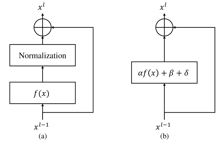
Figure 1: (a) A residual block with normalization layers, where $f(\cdot)$ denotes core computational primitive (e.g., convolution, attention, and aggregation). (b) NoMorelization replaces normalization layers with a learnable scalar-multiplier $\alpha$, bias $\beta$ and a zero-centered noise injector $\delta$.

Our main contributions are as follows:

• We find the regularization that current normalizer-free methods lack, namely noise injection from a sample’s perspective. By correcting the erroneous assumptions about the distribution of features, we model and derive the nature of injected noise and experimentally verify our assumptions.

• We propose a general normalizer-free method called NoMorelization. NoMorelization is composed of learnable scalars on the residual branch and a zero-centered Gaussian noise injector during training.

• NoMorelization outperforms mainstream normalizers and state-of-the-art normalizer-free methods in multiple backbones and tasks with better speed-accuracy trade-offs.

2 Related Works

2.1 Understanding Normalization Layers

Normalization Layers

Normalization layers standardize given input tensor $\boldsymbol{x}_{i}$ by Eq.1, i.e., minus input’s mean and divide it by its standard deviation (with a small positive number $\epsilon$). Then an optional affine transformation with a learnable mean $\beta$ and standard deviation $\gamma$.

$$\hat{\boldsymbol{x}}_{i}=\gamma\frac{\boldsymbol{x}_{i}-\mu}{\sqrt{\sigma^{2}+\epsilon}}+\beta$$ (1)

Several popular variants of normalization layers have been prevailing since their origin, including Batch Normalization (BN) (Ioffe and Szegedy 2015), Layer Normalization (LN) (Ba, Kiros, and Hinton 2016), Instance Normalization (IN) (Ulyanov, Vedaldi, and Lempitsky 2016), and Group Normalization (GN) (Wu and He 2018). The main difference among them is reflected in the statistics $\mu$ and $\sigma^{2}$.

Properties of Normalization Layers

Depending on the calculated statistics, Normalization layers have different properties. Different properties will cause different advantages and disadvantages, which is why it is difficult to design a general normalization layer.

• Global/Adaptive statistics. According to the way to gather, statistics can be divided into global and adaptive statistics. Global statistics are consistent for different samples and can be obtained through the moving average during training. In contrast, the statistics are unstable due to batch dependence (Labatie et al. 2021). The adaptive statistics are related to the sample, so the adaptive statistics must be gathered during inference. BN uses global statistics, while other methods (LN, IN, etc.) use adaptive statistics. Global statistics of BN can cause a training-inference discrepancy and lead to a decrease in model performance (Summers and Dinneen 2020; Wu and Johnson 2021).

• Unexpectedly Luxury Normalization is a surprisingly expensive computational primitive. It can occupy 25% of the total training time of a ResNet model (Gitman and Ginsburg 2017) and cause memory overhead (Bulò, Porzi, and Kontschieder 2018) for computing statistics.

• Complex Regularization It is widely believed that batch normalization also acts as a regularizer with noise injection (Luo et al. 2019; Liang et al. 2020). We can finetune the intensity of regularization by changing batch size. The smaller the batch size, the greater the intensity of regularization. In addition, researchers have found that normalization can smooth the lost landscape (Bjorck, Gomes, and Selman 2018), making the model have a certain degree of scaling invariance (Ulyanov, Vedaldi, and Lempitsky 2016), bias the model to its shallow path (De and Smith 2020a), orthogonalize the representations (Daneshmand, Joudaki, and Bach 2021), increases adversarial vulnerability (Benz, Zhang, and Kweon 2021), and so on.

2.2 Investigating Normalizer-Free (NF) Methods

There has been surging interest in designing normalizer-free methods. Through delicate initialization (Zhang, Dauphin, and Ma 2019), learnable scalar (De and Smith 2020b; Bachlechner et al. 2021), and scaled weight standardization (Brock, De, and Smith 2021), normalizer-free ResNets shows competitive results with BN ResNets. Recently (Brock et al. 2021) proposed a new NF backbone, namely NFNet. With adaptive gradient clipping, NFNet can outperform SOTA CNN-based models in ImageNet classification.

The Power of Down-scaling

Normalization is indispensable in modern residual blocks due to its ability to down-scale. Let $\boldsymbol{x}^{l}$ denotes the input batch of the $l$-th residual block, and $\boldsymbol{x}^{1}$ denotes the input of the model. A common assumption is that each sample of the network’s input is independently and identically distributed with Gaussian mean zero variance 1.

$$\mathbf{E}\left(\boldsymbol{x}_{i}^{1}\right)=0,\mathbf{Var}\left(\boldsymbol{x}_{i}^{1}\right)=1,$$ (2)

where the ${x}_{i}^{1}$ denotes the $i$-th sample of the input batch. The forward pass of $l$-th residual block is

$$\boldsymbol{x}^{l+1}=f^{l}(\boldsymbol{x}^{l})+\boldsymbol{x}^{l},$$ (3)

where $f^{l}(\cdot)$ is the composition of the layers and activation functions within the $l$-th block. With widely used ReLU activation (Glorot, Bordes, and Bengio 2011) and initialization method (such as Kaiming Init (He et al. 2015)), the layer outputs $f^{l}\left(x^{l}\right)$ are independent of their inputs, and thus the activations’ variance of an Unnormalized network grows exponentially with the number of blocks.

$$\mathbf{Var}\left(x_{i}^{l+1}\right)=\mathbf{Var}\left(x_{i}^{l}\right)+\mathbf{Var}\left(f_{i}^{l}\left(x^{l}\right)\right)\approx 2^{l}$$ (4)

Exponentially increasing activation variance can cause exploding gradients at the very beginning of training. But with normalization, the activation variance will be down-scaled to grow linearly.

$$\mathbf{Var}\left(x_{i}^{l+1}\right)=\mathbf{Var}\left(x_{i}^{l}\right)+\mathbf{Var}\left(\operatorname{Norm}(f_{i}^{l}\left(x^{l})\right)\right)=l+1$$ (5)

Therefore, existing NF works focus on stabilizing the outputs’ variance by initializing or introducing multipliers.

$$\boldsymbol{x}^{l+1}=\alpha\times f^{l}(\boldsymbol{x}^{l})+\boldsymbol{x}^{l},$$ (6)

where the $\alpha$ is a trainable parameter and initialized as 0. This multiplier helps the model to be normalized as an identity network and makes NF networks training possible.

Additional Regularization Effects

Despite the achievement in down-scaling, the NF models still suffer some accuracy loss than their Siamese with normalization. This is believed to be due to the additional regularization effect of normalization layers. NFNet (Brock et al. 2021) is the first NF model that achieves SOTA against the normalized. It claims that batch normalization can keep the model outputs’ mean to 0 and stabilize the numerical range of the gradient. To this end, NFNet implements scaled weight normalization and adaptive gradient clipping to the NF model.

3 NoMorelization: A Sample’s Perspective

The key motivation of NoMorelization is to rethink BN from a sample’s perspective and thus reveal the regularization effect REALLY MISSED in existing NF methods. The state-of-the-art NFNets (Brock et al. 2021) treat BN’s regularization as multiple complex regularization effects. However, from a sample’s perspective, we conclude that a very simple noise injector can be implemented as a surrogacy for BN to realize better normalizer-free modules. In the following sections, we empirically illustrate the irrationality of the regularization scheme of NFNet and provide a theoretical basis for the correctness of Noise Injection.

3.1 Why Noise Injection

Existing choices are not reasonable

	W/o Regularization	NF- Regularization	Improvement
BN-Net	92.47	93.23	0.76
NF-Net	92.00	92.51	0.51
$\Delta$Acc	0.47	0.72	0.25 ($\geq$0)

Table 1: The average accuracy improvement of the regularization in NFNet (Brock et al. 2021) is compared in the CIFAR-10 dataset of ResNet-110 with and without BN. The results show that the BN-Net receives a more noticeable improvement via NFNet’s regularization.

We implement two 110-layer ResNets. The first ResNet is implemented with BN and called BN-Net. The multiplier replaces the BN layers of the other ResNet described as Eq. (6). This network is called NF-Net. We then perform two sets of training on these two networks. The first set of training does not use any regularization for both networks. The second set is trained with the regularization used by the NFNets (Brock et al. 2021) (i.e., adaptive gradient clipping and scaled weight standardization). The average results are shown in Tab. 1. It is worth noting that NF-Net with additional NFNets-style regularization can surpass the performance of vanilla BN-Net, but the regularization can improve BN-Net even more. This intuitively shows that the existing regularization choice is a complement instead of a substitute for the BN regularization effect. Similar results can be found in more models and datasets in Tab. 2.

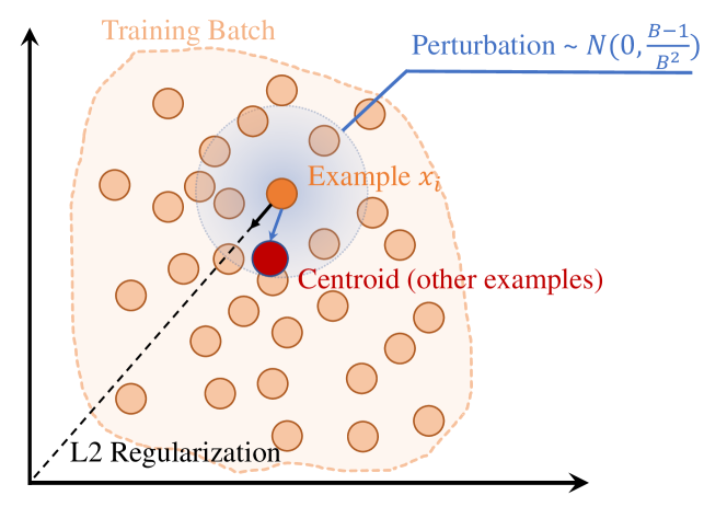
Figure 2: Batch normalization: a sample’s perspective (under the I.I.D. assumption)

Injected Noise Exists

Ignoring the learnable parameters(i.e. $\beta$ and $\gamma$) in Eq. 1, we deduce what BN has actually done from the perspective of the i-th sample $\boldsymbol{x}_{i}$. The previous work (De and Smith 2020b) has proved that the normalization methods can stabilize the variance of the output data. We assume that the standard deviation of the denominator can be discarded together with the learnable standard deviation $\gamma$ for brevity. To simplify the discussion, we consider the case where variables such as $x_{i}$ are scalars.

$$\hat{x_{i}} =x_{i}-\mu$$ (7)

$$=x_{i}-\frac{1}{B}\sum_{j=1}^{B}x_{j}$$

$$=x_{i}-\frac{1}{B}x_{i}-\frac{1}{B}\sum_{j=1,j\neq i}^{B}x_{j}$$

$$=\frac{B-1}{B}x_{i}-\frac{1}{B}\sum_{j=1,j\neq i}^{B}x_{j},$$

where $x$ are random variables that obey the standard normal distribution (via the definition of BN). Wherefore $\sum_{j=0}^{B-1}x_{j}\sim\mathcal{N}(0,B-1)$.

$$\hat{x_{i}}=\frac{B-1}{B}x_{i}-\delta,(\delta\sim\mathcal{N}(0,\frac{B-1}{B^{2}})).$$ (8)

The above formula is the so-called a sample’s perspective in BN. As shown in Fig. 2, BN firstly performs an L2 regularization on this sample (i.e., $\frac{B-1}{B}\boldsymbol{x}_{i}$), and then injects a random Gaussian perturbation $\delta$. The magnitudes of these two regularizing effects are both related to the batch size $B$. The larger the batch size, the smaller the magnitude of the regularization. This also explains the subtle relationship between the batch size and the corresponding test accuracy found in previous studies (He, Liu, and Tao 2019; Luo et al. 2019).

4 Noise Modeling

Although we claim that noise injection is an additional regularization effect of BN, the effects of sampling noise, which are mostly negative, have also been extensively studied. For example, using a fixed virtual batch can eliminate noise and improve performance (especially on generative models) (Salimans et al. 2016). Fixing the proportion of classes in each batch can also reduce noise and improve the performance in various tasks (Wu and Johnson 2021), e.t.c.

We are concerned about what the noise is and whether we can use it as a regularization. With the well-known two contradictory prior knowledge of previous works:

• Without BN’s extra regularization effects (including noise), the normalizer-free models suffer from a lower accuracy.

• Because BN has training noise, alleviating the “training noise” of BN will improve models’ performance (Gao et al. 2021).

In general, we believe that BN’s noise is beneficial to the training of deep learning models, but the noise is too large. The excessively large part of the noise is a polynomial distribution noise related to the sampling result. Removing this noise and leaving only the Gaussian noise with a mean value of zero is more helpful for model training.

Moreover, the existence of excessive noise is an important reason why BN cannot be generalized to all models and tasks. We can build a general NoMorelization by “distilling” the excessive noise, i.e., only injecting a small zero-centered noise during training.

4.1 Rewrite the Prior Distribution

We argue that the prior distribution of the input data should not obey an i.i.d. Gaussian distribution. If the model needs to extract meaningful representations for downstream tasks, the distribution of the extracted representations tends to be polycentric (Girshick et al. 2014). BN is also confirmed to require additional corrections when the non-iid situation is more severe (Li et al. 2021), and BN may fail with large variation (Lian and Liu 2019). The data should be composed of multiple Gaussian distributions, and the number of distributions in classification tasks is at least the number of classes. For dataset $\mathcal{D}=\{(x_{i},y_{i})\}$, $x\sim\mathcal{N}(\mu^{(y)},\sigma^{(y)2})$, where $y_{i}$ denotes the distribution (e.g. class) index of $i$-th sample.

4.2 Rewrite the Noise Model

With the modified prior distribution, we can rewrite the noise model in Eq. (7) as:

$$\hat{x_{i}} =\frac{B-1}{B}\tilde{x}_{i}^{y_{i}}-\delta,$$ (9)

$$\text{where }\tilde{x}_{i} \sim\mathcal{N}(\mu^{y_{i}},\sigma^{(y_{i})2}),$$

$$\delta \sim\mathcal{N}(\underbrace{\frac{1}{B}\sum_{j=1,j\neq i}^{B}\mu_{j}^{y_{j}}}_{\text{Inter-distribution}},\underbrace{\frac{1}{B^{2}}\sum_{j=1,j\neq i}^{B}\sigma^{(y_{j})2}}_{\text{Intra-distribution}}).$$

The sum of multiple independent Gaussian variables still follows a Gaussian distribution, but we can refer to the mean and variance parts of this Gaussian distribution as the Inter-distribution noise and the Intra-distribution noise, respectively. Now we are going to discuss the nature of rewrited noise in Eq. (9).

Inter-distribution Noise

Observe the mean value of the disturbance $\delta$, which is actually the summation of the expectation of each distribution sample. Because each sample in the batch is independent, we have

$$P\left\{|y=1|=m_{1},|y=2|=m_{2},\cdots,|y=n|=m_{n}\right\}=$$ (10)

$$\frac{B!}{m_{1}!m_{2}!\cdots m_{n}!}p_{1}^{m_{1}}p_{2}^{m_{2}}\ldots p_{n}^{m_{n}},$$

where $n$ is the number of distributions, and $B$ is the batch size. $|y=i|$ refers to the number of samples belonging to $i-$th distribution, also denoted as $m_{i}$, and $p_{i}$ is the probability of the $i$-th distribution being sampled (the same as the ratio of every distribution when the datasets is large enough). Each case of the above sampled polynomial distribution corresponds to a mean value of $\sum_{j=1,j\neq i}^{B}\mu_{j}^{y_{j}}$.

Because the mean value of this noise is also a random variable, when sampling time is large enough, it will be more like a Gaussian distribution approaching the same center, just like the previous noise model in Eq. (8). But for each BN sampling for training, the noise is indeed not zero-centered.

Intra-distribution Noise

After stripping the inter-distribution noise, the remainder becomes a zero-centered Gaussian noise $\mathcal{N}(0,\frac{1}{B^{2}}\sum_{j=1,j\neq i}^{B}\sigma^{(y_{j})2})$. We call it intra-distribution noise, and we assume that the standard deviation of this distribution is smaller than the range of inter-distribution noise. We will elaborate and verify our claims in subsequent assertions and experiments.

Special cases

The above formula is complicated, but we can propose special cases. For the $i-$th sample in a batch, if all samples except $i-$th belong to same distribution (no matter what $i$-th sample’s distribution is.) The noise term can be simplified as for: $\delta^{(y)}\sim\mathcal{N}(\frac{B-1}{B}\mu^{y},\frac{B-1}{B^{2}}\sigma^{(y)2})$. It can be vividly shown in Fig. 3. Samples perturbed by noise exhibit polycentric distributions related to the sampled class.

4.3 Assertions

Assertion 1: Intra-distribution noise extraction

If we fix a sample $x_{i}$ and sample other data from an arbitrary distribution of $y_{i}$ to form a batch and then perform BN, we can get the embeddings of $x_{i}$ represented by $\hat{x_{i}}(1),\cdots,\hat{x_{i}}(K)$ after repeated random sampling and applying BN for $K$ times. Then subtract two different $\hat{x_{i}}$ (e.g., $\hat{x_{i}}(3)-\hat{x_{i}}(4)$), the result should be:

$$\delta^{\prime}\sim\mathcal{N}(0,\frac{2B-2}{B^{2}}\sigma^{(y)2}).$$ (11)

In fact, $\delta^{\prime}$ obtained above should also be a zero-centered Gaussian distribution as long as the proportion of the batched samples belonging to each distribution is constant.

Assertion 2: Inter-distribution noise extraction

Based on Assertion 1, if the sampled batch data and the fixed sample $x_{i}$ are from the same distribution $y_{i}$ after $K$ sampling and BN, the exception of $\hat{x_{i}}$ should be described as:

$$E(\hat{x_{i}})_{\text{self}}=\frac{B-1}{B}\mu^{y_{i}}-\frac{B-1}{B}\mu^{y_{i}}=0.$$ (12)

And if not so, the exception is non-zero:

$$E(\hat{x_{i}})_{y}=\frac{B-1}{B}\mu^{y_{i}}-\frac{B-1}{B}\mu^{y}\neq 0.$$ (13)

Assertion 3: The noise decomposition assumption

The influence of BN is mainly dominated by inter-distribution noise. When we really calculate the noise caused by BN, we can distinguish which distribution the fixed sample is combined with according to the noise.

We validate our assertions by hypothesis test and visualization experiment in Sec. 5.1. We demonstrate that our assumptions about the prior distribution are more realistic by the three assertions.

4.4 NoMorelization

After clarifying the noise effect of BN, we give a simple formula for NoMorelization:

$$\alpha f(\boldsymbol{x})+\beta+\boldsymbol{\delta},$$ (14)

where the $\alpha$ and $\beta$ are multiplier and offset initialized as 0 like affine transformation in normalization layers in Eq. (1). $\boldsymbol{\delta}$ is a standard zero-centered Gaussian noise vector. In practice, we find that those backbones using BN tend to prefer larger noise, while those using LN and IN prefer smaller noise. So we multiply $\boldsymbol{\delta}$ by a scalar $\gamma$ as a hyperparameter, and we explain the hyperparameter further in Sec. 5.4.

$$\alpha f(\boldsymbol{x})+\beta+\gamma\times\boldsymbol{\delta},$$ (15)

In summary, by introducing a zero-centered Gaussian noise, our NoMorelization can achieve an elegant trade-off between speed and accuracy, i.e., NoMorelization is a substitute with a low cost and even exceed the performance of various normalization layers in accuracy. Moreover, our experimental results prove that, with nice interpretability, NoMorelization is more substitutable than complementary to the regularization effect of BN compared to existing normalizer-free methods. So we multiply delta by a scalar as a hyperparameter, and we explain the hyperparameter further in the experiments section.

Dataset	Backbone	Norm	NF-Norm	Fixup	SkipInit	NFNet	Ours	NF-Ours
CIFAR-10	ResNet	92.31 $\pm$ 0.36 (1 $\times$)	93.06 $\pm$ 0.26 (0.43 $\times$)	91.32 $\pm$ 0.40 (1.03 $\times$)	91.92 $\pm$ 0.32 (1.35 $\times$)	92.76 $\pm$ 0.39 (0.43 $\times$)	92.47 $\pm$ 0.35 (1.22 $\times$)	93.39 $\pm$ 0.30 (0.43 $\times$)
	ConvNeXt	88.47 $\pm$ 0.45 (1 $\times$)	89.59 $\pm$ 0.33 (0.62 $\times$)	88.75 $\pm$ 0.41 (1.20 $\times$)	88.23 $\pm$ 0.44 (1.29 $\times$)	89.92 $\pm$ 0.36 (0.59 $\times$)	89.08 $\pm$ 0.50 (1.13 $\times$)	90.26 $\pm$ 0.40 (0.57 $\times$)
	Swin	94.45 $\pm$ 0.13 (1 $\times$)	94.64 $\pm$ 0.03 (0.84 $\times$)	N/A N/A	94.23 $\pm$ 0.18 (1.11 $\times$)	94.81 $\pm$ 0.07 (0.88 $\times$)	94.72 $\pm$ 0.15 (1.11 $\times$)	94.85 $\pm$ 0.07 (0.87 $\times$)
CIFAR-100	ResNet	72.12 $\pm$ 0.31 (1 $\times$)	72.70 $\pm$ 0.36 (0.32 $\times$)	72.41 $\pm$ 0.64 (1.01 $\times$)	72.06 $\pm$ 0.60 (1.17 $\times$)	72.53 $\pm$ 0.37 (0.37 $\times$)	72.58 $\pm$ 0.41 (1.05 $\times$)	72.84 $\pm$ 0.36 (0.35 $\times$)
	ConvNeXt	66.37 $\pm$ 0.38 (1 $\times$)	68.01 $\pm$ 0.48 (0.88 $\times$)	66.04 $\pm$ 0.69 (1.41 $\times$)	65.11 $\pm$ 1.39 (1.17 $\times$)	67.79 $\pm$ 0.23 (0.68 $\times$)	67.20 $\pm$ 0.96 (1.17 $\times$)	69.05 $\pm$ 0.44 (0.64 $\times$)
	Swin	76.93 $\pm$ 0.17 (1 $\times$)	77.34 $\pm$ 0.14 (0.86 $\times$)	N/A N/A	76.79 $\pm$ 0.35 (1.11 $\times$)	77.18 $\pm$ 0.16 (0.88 $\times$)	77.14 $\pm$ 0.21 (1.10 $\times$)	77.26 $\pm$ 0.18 (0.84 $\times$)
Tiny-ImageNet	ResNet	61.29 $\pm$ 0.41 (1 $\times$)	60.68 $\pm$ 0.30 (0.70 $\times$)	61.32 $\pm$ 0.30 (1.02 $\times$)	61.41 $\pm$ 0.27 (1.16 $\times$)	59.36 $\pm$ 0.48 (0.78 $\times$)	61.56 $\pm$ 0.31 (1.10 $\times$)	60.59 $\pm$ 0.19 (0.71 $\times$)
	ConvNeXt	61.40 $\pm$ 0.59 (1 $\times$)	62.37 $\pm$ 0.37 (0.84 $\times$)	61.55 $\pm$ 0.68 (1.11 $\times$)	61.42 $\pm$ 0.62 (1.18 $\times$)	62.13 $\pm$ 0.57 (0.88 $\times$)	61.80 $\pm$ 0.56 (1.14 $\times$)	62.56 $\pm$ 0.53 (0.85 $\times$)
	Swin	58.12 $\pm$ 0.13 (1 $\times$)	58.41 $\pm$ 0.06 (0.90 $\times$)	N/A N/A	59.12 $\pm$ 0.23 (1.16 $\times$)	59.61 $\pm$ 0.08 (0.93 $\times$)	59.64 $\pm$ 0.26 (1.14 $\times$)	59.89 $\pm$ 0.13 (0.85 $\times$)

Table 2: Top-1 accuracy comparison on different datasets and backbones. The value in parentheses is the speedup ratio compared to its normalizer baseline. Bold denotes the highest accuracy, italic denotes exceeding the normalizer baseline in both accuracy and speed.

5 Experiments

Experiments in this paper are run on an Ubuntu 16.04 LTS server with 8$\times$NVIDIA Tesla P100 (16GB) GPUs. We implement all deep learning models based on PyTorch 1.7.1 (Paszke et al. 2017) with Cuda 10.2. We provide the core python implementation of NoMorelization in Appendix A.

5.1 Assertions Tests

We select a cat picture as an invariant sample $x_{i}$ in CIFAR-10 (Krizhevsky, Hinton et al. 2009) dataset, and use Hotelling’s $T^{2}$ hypothesis test (Hotelling 1992) to validate our assertions. It is worth mentioning that we use a trained ResNet in the following assertions testing, so the differences between different embedding results for the invariant sample are only due to the sampling noise in the batch. See Appendix LABEL:app:test for more details and results.

Assertion test 1

We divide the images of each category in the dataset into 40 parts and choose a category arbitrarily. The invariant samples are concatenated with 50 parts of pictures to form 40 batches. By feeding the batches into a ResNet-56 model in training mode, we can get 40 random samples of 64-dim embedding vector of the invariant cat $\hat{\boldsymbol{x}_{i}}(1),\cdots,\hat{\boldsymbol{x}_{i}}(40)$. After that, we subtract the embeddings of different sampling indexes to get $C^{2}_{40}=780$ sets of sampled intra-class noise. We perform a one-sample test between sampled intra-class noise and a zero matrix.

Assertion test 2

We set the batch size to 128 and randomly sample from the same class 1000 times, concatenate them with the invariant sample and then get 1000 different $\hat{\boldsymbol{x}_{i}}$ samples for ten classes. Moreover, we test them with a zero matrix respectively for hypothesis testing.

Assertion test 3

We perform Principal Component Analysis (PCA) on $\hat{\boldsymbol{x}_{i}}$ for each class used in Assertion 1. As shown in Fig. 3, the embedding shift of the invariant sample will be dominated by the inter-class noise especially when the samples are all of the same distribution (class). There is also slight intra-class noise within each class.

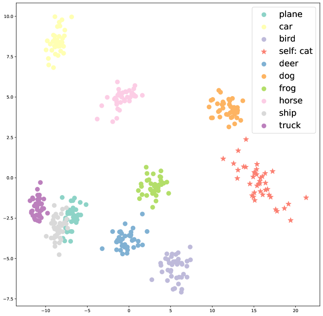
Figure 3: PCA results of the $\hat{\boldsymbol{x}_{i}}$ of the invariant cat sample within a batch of different distributions. The special case of inter-class noise and intra-class noise are shown vividly.

5.2 Image Classification

Datasets and baselines.

We perform image classification experiments on four datasets, including three tiny image datasets (i.e., CIFAR-10, CIFAR-100 (Krizhevsky, Hinton et al. 2009) and Tiny-ImageNet (Le and Yang 2015)) and a standard ImageNet (Deng et al. 2009) dataset. To evaluate the generality of NoMorelization, we choose three types of backbone: ResNet-56 as a classical CNN with BN, ConvNeXt (Liu et al. 2022) as a state-of-art CNN architecture with LN, and Swin-Transformer (Liu et al. 2021) as recently mainstream attention-based model. As far as we know, the current attention-based models all use LN. Please refer to Appendix LABEL:app:class for detailed model design and hyper-parameter settings.

Experimental Results.

We train all models with different random seeds five times and compute the mean and standard deviation of top-1 accuracy. In order to compare the efficiency of different methods, we also record the average time-consuming of five training sessions. The accuracy and speed are recorded in Tab. 2. NoMorelization is the only method that can exceed the normalizer baseline in both accuracy and speed across all backbones and datasets. Furthermore, the highest accuracy can be obtained by NoMorelization in most cases with the additional regularization of NFNets, if training speed is not a concern. Finally, it is worth mentioning that Fixup initialization (Zhang, Dauphin, and Ma 2019) is designed for ResNet. Although Fixup initialization can achieve good results on CNN-based backbones, applying it to Transformer-based backbones will make the model difficult to converge.

Evaluating on ImageNet.

We also implement a standard ResNet-50 to evaluate the performance of different methods on a large-scale dataset. As shown in Fig. 4, only NFNet and our NoMorelizaion can outperform the BN baseline. The additional regularization of NFNet, as we mentioned in Sec. 3.1, is not a replacement for BN but a complement. That means using NFNet-like gradient clipping and weight standardization along with our NoMorelization can improve performance and get the best results.

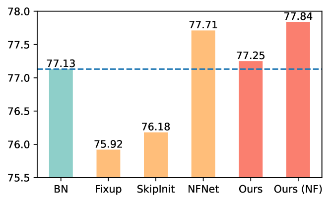
Figure 4: Top-1 Acc on ImageNet dataset with ResNet-50. Ours (NF) means we perform additional gradient clipping and weight standardization like NFNets. The green, yellow, and red bars represent the normalizer baseline, existing NF methods (i.e., Fixup, SkipInit (De and Smith 2020b), and NFNet), and NoMorelization, respectively.

	summer2winter		horse2zebra
	FID $\downarrow$	IS $\uparrow$	FID $\downarrow$	IS $\uparrow$
IN	83.72	2.78	64.52	1.42
NoMorelization	81.83	2.83	63.00	1.50

Table 3: Quantitative comparison of generative tasks.

(a) Input horse

(b) IN

(c) NoMorelization

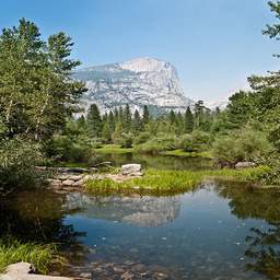
(d) Input summer

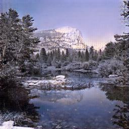
(e) IN

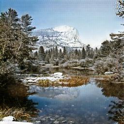
(f) NoMorelization

Figure 5: Qualitative comparison of generative tasks.

5.3 Image-to-Image Translation

To verify the effect of NoMorelization on generative tasks, we implement CycleGAN (Zhu et al. 2017) based on MMGeneration (Contributors 2021). CycleGAN is a GAN model applied to image-to-image translation tasks. CycleGAN uses Instance Normalization by default. First, we train a standard CycleGAN model on the Summer-to-Winter and Horse-to-Zebra datasets. Then we replace IN in CycleGAN with NoMorelization. Finally, we perform quantitative and qualitative comparisons of CycleGAN using IN and NoMorelization. We train CycleGANs for 250k iterations. For quantitative comparison, we generate 128 images after every 10k iterations of training and calculate their Frechet Inception Distance (FID) (Heusel et al. 2017) and Inception Score (IS) (Barratt and Sharma 2018). Lower FID and higher IS indicate better results. We report the lowest FID obtained by the models and the IS at this time, as shown in Tab. 3. NoMorelization outperforms the IN baseline in quantitative scores under the same hyperparameter settings. For qualitative comparison, we run the CycleGAN checkpoint in Tab. 3 on the test set. Results are shown in Fig. 5. On two tasks, the generative models with NoMorelization perform well intuitively compared to the IN baselines. More NoMorelization-based generation results and training settings are in Appendix LABEL:app:generate.

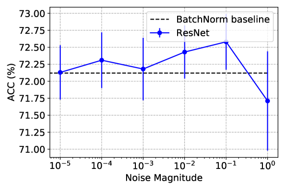
(a) Sensitivity analysis on ResNet

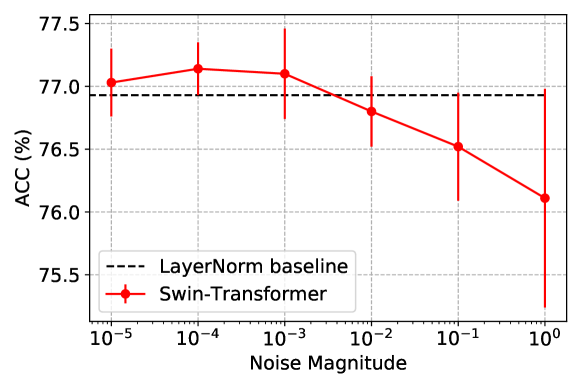
(b) Sensitivity analysis on Swin-Transformer

Figure 6: Sensitivity analysis on noise amplitude. We choose ResNet and Swin-Transformer on the CIFAR-100 dataset as examples. The black line represents the normalizer baseline.

5.4 In-depth Analysis

To determine the appropriate noise for different model architectures, we performed a log-scale grid search for magnitude among $[1,1e-1,\cdots,1e-5]$ on different backbones. As a result, we find that different backbones have different sensitivity of noise injected by NoMorelization. BN-based backbones can tolerate more extensive noise (i.e., 1e-1), while LN-based backbones prefer smaller noise amplitudes (i.e., 1e-4). We take the BN-based ResNet and LN-based Swin-Transformer as examples. As shown in Fig. 6(a), ResNet backbone with NoMorelization easily exceeds the BN baseline. Such advantages are more pronounced when the noise amplitude gradually increases from 1e-5 to 1e-1. However, if the magnitude of injected noise is too large (i.e., 1), the accuracy of NoMorelization will drop rapidly and make the training results unstable. For the Swin-Transformer shown in Fig. 6(b), although NoMorelization can achieve higher accuracy than its baseline, the accuracy drop at early stage. The noise starts to have negative effects on the model when its magnitude reaches 1e-2.

The results of the sensitivity analysis also explain why we prefer BN as a normalizer for CNN-based architectures and LN for Transformer-based architectures. As the only common normalizer that introduces sampling noise, BN brings a greater noise regularization effect than NoMorelization. For noise-sensitive architectures (such as Transformer), the regularization of BN is too strong. Therefore, normalizers that do not introduce noise regularization (e.g., LN and IN) are chosen when implementing these models.

6 Conclusion

In this paper, we propose a simple and effective alternative to normalization, namely “NoMorelization”, by explaining BN’s effects from a sample’s perspective. NoMorelization is composed of two trainable scalars and a zero-centered noise injector. The experimental results validate our assumptions about the injected noise and show that NoMorelization is a general component of deep learning and is suitable for different model paradigms to tackle different tasks. Furthermore, compared with existing mainstream normalizers and state-of-the-art normalizer-free methods, NoMorelization shows the best speed-accuracy trade-off.

Appendix A NoMorelization Implementation

A.1 Environment

Hardware.

Experiments in this paper are run on an Ubuntu 16.04 LTS server with 8$\times$NVIDIA Tesla P100 (16GB) GPUs, Intel(R) Xeon(R) Gold 5115 CPU @2.40GHz, and 252 GB memory.

Software.

We implement all deep learning models based on Python 3.8.10, PyTorch 1.7.1 (Paszke et al. 2017) with Cuda 10.2, torchvision 0.8.2, mmcv 1.6.0, mmgeneration 0.7.1, and their dependencies.

A.2 Image Classification

For a fair comparison, we implement NoMorelization’s experiment based on existing open source code. The original code can be found in the comments in the code block below.

[!h] # NoMorelization ResNet Block # Modified from https://github.com/hongyi-zhang/Fixup class BasicBlock(nn.Module): def __init__(self, inplanes, planes, stride=1, downsample=None): super(BasicBlock, self).__init__() # Both self.conv1 and self.downsample layers downsample the input when stride != 1 self.conv1 = conv3x3(inplanes, planes, stride) self.relu = nn.ReLU(inplace=True) self.conv2 = conv3x3(planes, planes) self.downsample = downsample self.alpha = nn.Parameter(torch.zeros(1)) self.beta = nn.Parameter(torch.zeros(1))

def forward(self, x): identity = x out = self.conv1(x) out = self.relu(out) out = self.conv2(out) out = out * self.alpha + self.beta if self.training: out += torch.randn_like(out, device=out.device) * 0.1 if self.downsample is not None: identity = self.downsample(x) identity = torch.cat((identity, torch.zeros_like(identity)), 1) out += identity out = self.relu(out) return out

[!h] # NoMorelization ConvNeXt Block # Modified from https://github.com/facebookresearch/ConvNeXt class Block(nn.Module): def __init__(self, dim, drop_path=0., layer_scale_init_value=1e-6): super().__init__() self.dwconv = nn.Conv2d(dim, dim, kernel_size=7, padding=3, groups=dim) self.pwconv1 = nn.Conv2d(dim, 4 * dim, kernel_size=1) self.act = nn.GELU() self.pwconv2 = nn.Conv2d(4 * dim, dim, kernel_size=1) self.gamma = nn.Parameter(layer_scale_init_value * torch.ones((dim)), requires_grad=True) if layer_scale_init_value ¿ 0 else None self.alpha = nn.Parameter(torch.zeros(1)) self.beta = nn.Parameter(torch.zeros(1)) self.drop_path = DropPath(drop_path) if drop_path ¿ 0. else nn.Identity()

def forward(self, x): identity = x x = self.dwconv(x) x = self.pwconv1(x) x = self.act(x) x = self.pwconv2(x) if self.gamma is not None: x = self.gamma * x x = x * self.alpha + self.beta if self.training: x += torch.randn_like(x, device=x.device) * 1e-4 x = identity + self.drop_path(x) return x [!h] # NoMorelization Swin-Transformer Block # Modified from https://github.com/aanna0701/SPT_LSA_ViT class SwinTransformerBlock(nn.Module): def __init__(self, dim, input_resolution, num_heads, window_size=7, shift_size=0, mlp_ratio=4., qkv_bias=True, qk_scale=None, drop=0., attn_drop=0., drop_path=0., act_layer=nn.GELU, is_LSA=False): super().__init__() self.dim = dim self.input_resolution = input_resolution self.num_heads = num_heads self.window_size = window_size self.shift_size = shift_size self.mlp_ratio = mlp_ratio if min(self.input_resolution) ¡= self.window_size: self.shift_size = 0 self.window_size = min(self.input_resolution) assert 0 ¡= self.shift_size ¡ self.window_size, ”shift_size must in 0-window_size”

self.attn = WindowAttention( dim, window_size=to_2tuple(self.window_size), num_heads=num_heads, qkv_bias=qkv_bias, qk_scale=qk_scale, attn_drop=attn_drop, proj_drop=drop, is_LSA=is_LSA)

self.drop_path = DropPath(drop

References

- Ba, Kiros, and Hinton (2016) Ba, J.; Kiros, J. R.; and Hinton, G. E. 2016. Layer Normalization. ArXiv, abs/1607.06450.
- Bachlechner et al. (2021) Bachlechner, T.; Majumder, B. P.; Mao, H. H.; Cottrell, G.; and McAuley, J. J. 2021. ReZero is all you need: fast convergence at large depth. In UAI, volume 161 of Proceedings of Machine Learning Research, 1352–1361. AUAI Press.
- Barratt and Sharma (2018) Barratt, S. T.; and Sharma, R. 2018. A Note on the Inception Score. CoRR, abs/1801.01973.
- Benz, Zhang, and Kweon (2021) Benz, P.; Zhang, C.; and Kweon, I. S. 2021. Batch Normalization Increases Adversarial Vulnerability and Decreases Adversarial Transferability: A Non-Robust Feature Perspective. In ICCV, 7798–7807. IEEE.
- Bjorck, Gomes, and Selman (2018) Bjorck, J.; Gomes, C. P.; and Selman, B. 2018. Understanding Batch Normalization. In NeurIPS.
- Brock, De, and Smith (2021) Brock, A.; De, S.; and Smith, S. L. 2021. Characterizing signal propagation to close the performance gap in unnormalized ResNets. In ICLR. OpenReview.net.
- Brock et al. (2021) Brock, A.; De, S.; Smith, S. L.; and Simonyan, K. 2021. High-Performance Large-Scale Image Recognition Without Normalization. In ICML, volume 139 of Proceedings of Machine Learning Research, 1059–1071. PMLR.
- Bulò, Porzi, and Kontschieder (2018) Bulò, S. R.; Porzi, L.; and Kontschieder, P. 2018. In-Place Activated BatchNorm for Memory-Optimized Training of DNNs. In CVPR, 5639–5647. Computer Vision Foundation / IEEE Computer Society.
- Contributors (2021) Contributors, M. 2021. MMGeneration: OpenMMLab Generative Model Toolbox and Benchmark. https://github.com/open-mmlab/mmgeneration.
- Daneshmand, Joudaki, and Bach (2021) Daneshmand, H.; Joudaki, A.; and Bach, F. R. 2021. Batch Normalization Orthogonalizes Representations in Deep Random Networks. In NeurIPS, 4896–4906.
- De and Smith (2020a) De, S.; and Smith, S. L. 2020a. Batch Normalization Biases Deep Residual Networks Towards Shallow Paths. CoRR, abs/2002.10444.
- De and Smith (2020b) De, S.; and Smith, S. L. 2020b. Batch Normalization Biases Residual Blocks Towards the Identity Function in Deep Networks. In NeurIPS.
- Deng et al. (2009) Deng, J.; Dong, W.; Socher, R.; Li, L.-J.; Li, K.; and Fei-Fei, L. 2009. Imagenet: A large-scale hierarchical image database. In 2009 IEEE conference on computer vision and pattern recognition, 248–255. Ieee.
- Devlin et al. (2019) Devlin, J.; Chang, M.; Lee, K.; and Toutanova, K. 2019. BERT: Pre-training of Deep Bidirectional Transformers for Language Understanding. In NAACL-HLT (1), 4171–4186. Association for Computational Linguistics.
- Gao et al. (2021) Gao, S.; Han, Q.; Li, D.; Cheng, M.-M.; and Peng, P. 2021. Representative Batch Normalization with Feature Calibration. 2021 IEEE/CVF Conference on Computer Vision and Pattern Recognition (CVPR), 8665–8675.
- Girshick et al. (2014) Girshick, R. B.; Donahue, J.; Darrell, T.; and Malik, J. 2014. Rich Feature Hierarchies for Accurate Object Detection and Semantic Segmentation. 2014 IEEE Conference on Computer Vision and Pattern Recognition, 580–587.
- Gitman and Ginsburg (2017) Gitman, I.; and Ginsburg, B. 2017. Comparison of Batch Normalization and Weight Normalization Algorithms for the Large-scale Image Classification. ArXiv, abs/1709.08145.
- Glorot, Bordes, and Bengio (2011) Glorot, X.; Bordes, A.; and Bengio, Y. 2011. Deep Sparse Rectifier Neural Networks. In Gordon, G. J.; Dunson, D. B.; and Dudík, M., eds., Proceedings of the Fourteenth International Conference on Artificial Intelligence and Statistics, AISTATS 2011, Fort Lauderdale, USA, April 11-13, 2011, volume 15 of JMLR Proceedings, 315–323. JMLR.org.
- He, Liu, and Tao (2019) He, F.; Liu, T.; and Tao, D. 2019. Control Batch Size and Learning Rate to Generalize Well: Theoretical and Empirical Evidence. In Wallach, H. M.; Larochelle, H.; Beygelzimer, A.; d’Alché-Buc, F.; Fox, E. B.; and Garnett, R., eds., Advances in Neural Information Processing Systems 32: Annual Conference on Neural Information Processing Systems 2019, NeurIPS 2019, December 8-14, 2019, Vancouver, BC, Canada, 1141–1150.
- He et al. (2015) He, K.; Zhang, X.; Ren, S.; and Sun, J. 2015. Delving Deep into Rectifiers: Surpassing Human-Level Performance on ImageNet Classification. In 2015 IEEE International Conference on Computer Vision, ICCV 2015, Santiago, Chile, December 7-13, 2015, 1026–1034. IEEE Computer Society.
- He et al. (2016) He, K.; Zhang, X.; Ren, S.; and Sun, J. 2016. Deep Residual Learning for Image Recognition. In CVPR, 770–778. IEEE Computer Society.
- Heusel et al. (2017) Heusel, M.; Ramsauer, H.; Unterthiner, T.; Nessler, B.; and Hochreiter, S. 2017. GANs Trained by a Two Time-Scale Update Rule Converge to a Local Nash Equilibrium. In Guyon, I.; von Luxburg, U.; Bengio, S.; Wallach, H. M.; Fergus, R.; Vishwanathan, S. V. N.; and Garnett, R., eds., Advances in Neural Information Processing Systems 30: Annual Conference on Neural Information Processing Systems 2017, December 4-9, 2017, Long Beach, CA, USA, 6626–6637.
- Hotelling (1992) Hotelling, H. 1992. The generalization of Student’s ratio. In Breakthroughs in statistics, 54–65. Springer.
- Ioffe and Szegedy (2015) Ioffe, S.; and Szegedy, C. 2015. Batch Normalization: Accelerating Deep Network Training by Reducing Internal Covariate Shift. In ICML.
- Krizhevsky, Hinton et al. (2009) Krizhevsky, A.; Hinton, G.; et al. 2009. Learning multiple layers of features from tiny images.
- Labatie et al. (2021) Labatie, A.; Masters, D.; Eaton-Rosen, Z.; and Luschi, C. 2021. Proxy-Normalizing Activations to Match Batch Normalization while Removing Batch Dependence. In NeurIPS, 16990–17006.
- Le and Yang (2015) Le, Y.; and Yang, X. 2015. Tiny imagenet visual recognition challenge. CS 231N, 7(7): 3.
- Li et al. (2021) Li, X.; Jiang, M.; Zhang, X.; Kamp, M.; and Dou, Q. 2021. FedBN: Federated Learning on Non-IID Features via Local Batch Normalization. In ICLR. OpenReview.net.
- Lian and Liu (2019) Lian, X.; and Liu, J. 2019. Revisit Batch Normalization: New Understanding and Refinement via Composition Optimization. In Chaudhuri, K.; and Sugiyama, M., eds., The 22nd International Conference on Artificial Intelligence and Statistics, AISTATS 2019, 16-18 April 2019, Naha, Okinawa, Japan, volume 89 of Proceedings of Machine Learning Research, 3254–3263. PMLR.
- Liang et al. (2020) Liang, S.; Huang, Z.; Liang, M.; and Yang, H. 2020. Instance Enhancement Batch Normalization: an Adaptive Regulator of Batch Noise. In AAAI.
- Liu et al. (2021) Liu, Z.; Lin, Y.; Cao, Y.; Hu, H.; Wei, Y.; Zhang, Z.; Lin, S.; and Guo, B. 2021. Swin Transformer: Hierarchical Vision Transformer using Shifted Windows. In ICCV, 9992–10002. IEEE.
- Liu et al. (2022) Liu, Z.; Mao, H.; Wu, C.-Y.; Feichtenhofer, C.; Darrell, T.; and Xie, S. 2022. A ConvNet for the 2020s. Proceedings of the IEEE/CVF Conference on Computer Vision and Pattern Recognition (CVPR).
- Luo et al. (2019) Luo, P.; Wang, X.; Shao, W.; and Peng, Z. 2019. Towards Understanding Regularization in Batch Normalization. ArXiv, abs/1809.00846.
- Paszke et al. (2017) Paszke, A.; Gross, S.; Chintala, S.; Chanan, G.; Yang, E.; DeVito, Z.; Lin, Z.; Desmaison, A.; Antiga, L.; and Lerer, A. 2017. Automatic differentiation in PyTorch.
- Salimans et al. (2016) Salimans, T.; Goodfellow, I. J.; Zaremba, W.; Cheung, V.; Radford, A.; and Chen, X. 2016. Improved Techniques for Training GANs. In Lee, D. D.; Sugiyama, M.; von Luxburg, U.; Guyon, I.; and Garnett, R., eds., Advances in Neural Information Processing Systems 29: Annual Conference on Neural Information Processing Systems 2016, December 5-10, 2016, Barcelona, Spain, 2226–2234.
- Santurkar et al. (2018) Santurkar, S.; Tsipras, D.; Ilyas, A.; and Madry, A. 2018. How Does Batch Normalization Help Optimization? In NeurIPS.
- Summers and Dinneen (2020) Summers, C.; and Dinneen, M. J. 2020. Four Things Everyone Should Know to Improve Batch Normalization. In ICLR. OpenReview.net.
- Ulyanov, Vedaldi, and Lempitsky (2016) Ulyanov, D.; Vedaldi, A.; and Lempitsky, V. S. 2016. Instance Normalization: The Missing Ingredient for Fast Stylization. CoRR, abs/1607.08022.
- Vaswani et al. (2017) Vaswani, A.; Shazeer, N.; Parmar, N.; Uszkoreit, J.; Jones, L.; Gomez, A. N.; Kaiser, L.; and Polosukhin, I. 2017. Attention is All you Need. In NIPS, 5998–6008.
- Wu and He (2018) Wu, Y.; and He, K. 2018. Group Normalization. In ECCV.
- Wu and Johnson (2021) Wu, Y.; and Johnson, J. 2021. Rethinking ”Batch” in BatchNorm. CoRR, abs/2105.07576.
- Zhang, Dauphin, and Ma (2019) Zhang, H.; Dauphin, Y. N.; and Ma, T. 2019. Fixup Initialization: Residual Learning Without Normalization. In ICLR (Poster). OpenReview.net.
- Zhu et al. (2017) Zhu, J.-Y.; Park, T.; Isola, P.; and Efros, A. A. 2017. Unpaired image-to-image translation using cycle-consistent adversarial networks. In Proceedings of the IEEE international conference on computer vision, 2223–2232.