Importance Sampling Methods for Bayesian Inference with Partitioned Data

Abstract

This article presents new methodology for sample-based Bayesian inference when data are partitioned and communication between the parts is expensive, as arises by necessity in the context of “big data” or by choice in order to take advantage of computational parallelism. The method, which we call the Laplace enriched multiple importance estimator, uses new multiple importance sampling techniques to approximate posterior expectations using samples drawn independently from the local posterior distributions (those conditioned on isolated parts of the data). We construct Laplace approximations from which additional samples can be drawn relatively quickly and improve the methods in high-dimensional estimation. The methods are “embarrassingly parallel”, make no restriction on the sampling algorithm (including MCMC) to use or choice of prior distribution, and do not rely on any assumptions about the posterior such as normality. The performance of the methods is demonstrated and compared against some alternatives in experiments with simulated data.

Keywords: big data; parallel computing; Bayesian inference; Markov chain Monte Carlo; embarrassingly parallel; federated inference; multiple importance sampling

1 Introduction

Bayesian sample-based computation is a common approach to Bayesian inference in non-trivial models where it is infeasible to compute the normalising constant of the posterior distribution. The focus of this article is on performing Bayesian computation when data are partitioned and communication between the parts is expensive or impossible. We present new methodology for Bayesian inference in this context without having to combine the parts and communicating between the parts only at the end of sampling. Our methods achieve this with competitive performance and with fewer constraints or assumptions than some other methods.

Bayesian computation with partitioned data is challenging because the algorithms for generating samples from the posterior typically require many calculations involving the whole data set; specifically, likelihood evaluations. For example, in Markov chain Monte Carlo (MCMC) algorithms such as the Metropolis-Hastings algorithm, a (typically large) number of dependent samples are generated from a Markov chain, each constrained by the previous sample and the data (see e.g. Robert and Casella, (2004)). When used to target a posterior distribution $\pi\left(\theta\mid x\right)$ given data $x$, the probability of accepting proposal $\theta^{\prime}$ given $x$ and previous sample $\theta$ is

$$\min\left(\frac{\pi\left(\theta^{\prime}\mid x\right)}{\pi\left(\theta\mid x\right)}\frac{q\left(\theta\mid\theta^{\prime}\right)}{q\left(\theta^{\prime}\mid\theta\right)},1\right),$$ (1)

where $q$ is the density of the proposal distribution. The ratio $\frac{\pi\left(\theta^{\prime}\mid x\right)}{\pi\left(\theta\mid x\right)}$ (which may be of unnormalised p.d.f.s because the normalising constant cancels) must be evaluated for every proposal $\theta^{\prime}$, i.e. in every iteration. Even if observations are conditionally independent given $\theta$, so that likelihoods evaluated using parts of the data can be multiplied to give the full data likelihood, this can still be a problem if the necessary data transfer is expensive or impossible.

There are three important data analysis situations where data are partitioned:

1. When a data set is too large to work with in the memory of one computer.

2. When there are several sources or owners of data which are unable or unwilling to share their data.

3. When there is the possibility of speeding up sampling by running multiple instances of the sampling algorithm in parallel on separate parts of the data.

The first situation arises in the context of “big data”: data that must be stored in a distributed manner with no shared memory for computing. Big data has become very important in modern science and business because of the possibility of finding patterns not observable on a smaller scale and which may lead to deeper understanding or provide a competitive edge (Bryant et al., (2008); Sagiroglu and Sinanc, (2013)). The open source Apache Hadoop framework is widely used for storing and computing with big data on a cluster (Apache Hadoop, (2018); Borthakur, (2007)). In the Hadoop file system (HDFS), data are partitioned into “blocks” and stored across the cluster, in duplicate for resilience to errors, then processed using parallel computation models such as MapReduce (Dean and Ghemawat, (2008)) and Spark (Zaharia et al., (2010)) which operate on data using memory local to each block. A major source of inefficiency in these computations arises when data must be communicated between cluster nodes (Kalavri and Vlassov, (2013); Sarkar et al., (2015)).

One possible approach to Bayesian computation in this context is to down-sample the data to a size that will fit in the local memory of one computer, but down-sampling a large data set seems to defeat the purpose of collecting it in the first place. As pointed out in Scott et al., (2016), some large, complex models genuinely require a large amount of data for robust estimation.

The second situation arises due to data privacy concerns or in meta-analyses. Inference in this situation is sometimes known as “federated inference” (and the distributed data, “federated data”) (Xiong et al., (2021); Ma et al., (2021)). Current approaches to preserving privacy often rely on the masking of data or the addition of noise (Dwork, (2008); Torra and Navarro-Arribas, (2016)), both which imply the loss of information. Meta-analyses use statistical procedures such as mixed effects models to pool the results of primary studies using aggregated data when there is no access to raw observational data (DerSimonian and Laird, (1986)). Performing inference in global models for pooled data without any participants having to share their data may open up new possibilities in these situations.

In the third situation, we may assume there is ample memory for the entire data set, but computational parallelism is available such as through multiple CPU cores, with a GPU or array of GPUs (Lee et al., (2010)), or on a cluster, and the time complexity of the sampling algorithm depends on the number of data points. In this situation there is an opportunity to generate more samples in a given time by running the sampler in parallel on subsets of the data. This may result in estimators with lower bias and variance than would otherwise be possible.

If the data can be contained in the memory of a single node, another way of taking advantage of computational parallelism is to run multiple MCMC chains in parallel. Besides the large number of samples that can be generated (e.g. Lao et al., (2020)), there is potential for improved convergence and new adaptive algorithms (Green et al., (2015)). This is a different mode of parallelism and not the concern of this paper.

Our approach is for each worker node (the cluster node or agent managing each data part) to run the same sampling algorithm independently on their local data, resulting in sets of samples from posterior distributions different from the full data posterior distribution. We regard these local posteriors as importance proposal distributions or components of a mixture proposal distribution targeting the posterior (Robert and Casella, (2004); Owen, (2013)). By correctly weighting the samples we can construct Monte Carlo estimators of a posterior expectation that are asymptotically unbiased in the sense of approaching zero bias in the limit of infinite samples. There are two observations that suggest importance sampling-based estimation in this context may be fruitful. Firstly, the local posteriors should be similar to the posterior (so long as the parts of data are similar in distribution); secondly, the tails of the local posteriors should be fatter than those of the posterior because they are conditioned on less data (see e.g. MacKay et al., (2003)). We make use of three importance weighting strategies which fit into the class of multiple importance sampling (Veach and Guibas, (1995); Hesterberg, (1995); Owen, (2013); Elvira and Martino, (2021)). Two of these strategies we devised by extending the methods of Veach and Guibas, (1995) to the case where both the target density and the proposal densities are only known up to a constant of proportionality. The third strategy we believe is novel.

Importance sampling is known to suffer the curse of dimensionality, leading to poor performance in high-dimensional models (MacKay et al., (2003)). To address this we include samples from Laplace approximations to the posterior to complement the samples received from the workers. These additional samples can be generated easily without additional iterations of the posterior sampling algorithm, which are often relatively costly. The approximations are simple constructions from the pooled samples that provide additional importance proposals which, it is hoped, cover regions of parameter space not covered by the local posteriors. We consider three ways of doing this, but find that only one of them is particularly useful in the majority of examples.

The advantages of our methods can be summarised as follows. They appear to perform relatively well (comparing with some alternative approaches) in terms of approximating posterior expectations across a range of models, and in particular for non-normal posteriors. We will provide evidence of this from experiments with synthetic data. Our methods have no preference of algorithm used for sampling by the workers using local data, so long as it is approximately unbiased, and no communication between workers is required until the very end of the sampling. This means we can perform sampling in an “embarrassingly parallel” fashion (Herlihy et al., (2020)). In fact, no data (i.e. observations) need be transmitted between nodes at all (after any initial partitioning of data). This is an essential requirement in the use case of collaboration between parties who are unable to share data, and is an advantage to parallel computation on a cluster where data transfer between nodes is a performance bottleneck. Our methods can be used without any constraint on the choice of prior distribution. This is in contrast to some other methods, in which it is necessary that the prior be amenable to a certain transformation for the methods to be unbiased. This constrains the choices available for the prior in those methods, which can have unwanted implications for the analysis, particularly in analyses of small data sets. There are also no hyperparameters that need to be set or tuned in our methods.

We make no distributional assumptions about the posterior. The only assumptions we need beyond those implied by the model or the sampling algorithm are that observations which are held in separate parts are conditionally independent of each other given model parameters, that the likelihood function is computable and the mild assumptions required by importance sampling. Conditional independence of all observations is sufficient but stronger than necessary. However, whilst we make no explicit assumptions against non-random partitioning of the data, random partitioning would likely be beneficial for methods based on importance sampling because it makes the local posteriors more likely to resemble the posterior. We do not require the size of the data parts to be equal or the number of samples drawn by each worker to be equal.

There are two useful performance diagnostics we propose to use with our methods. First, we derive an effective sample size in the manner of Kong, (1992). This is a measure of the sampling efficiency lost due to the use of an approximation. Second, we look at the $\hat{{k}}$ diagnostic arising in the Pareto smoothed importance estimator of Vehtari et al., (2015). This is an estimate of the shape parameter in a generalised Pareto model for the tail of the importance weight distribution, for which Vehtari et al., (2015) identified a threshold which seems to be a valuable indicator of poor performance. We find that, together, these indicate situations where our estimators perform poorly.

As of writing, the problem of Bayesian inference with partitioned data remains an open challenge (Green et al., (2015); Bardenet et al., (2017)), although there are some notable contributions. Some hierarchical models have a structure that is particularly amenable to distributed processing, such as the hierarchical Dirichlet process topic model, for which Newman et al., (2009) devise a distributed Gibbs sampling algorithm. This approach does not generalise to other models, however.

A number of methods start from the observation that the posterior density is proportional to the product of local posterior densities, the product distribution, under a conditional independence assumption for the data. Scott et al., (2016) make normal distribution assumptions for the local posteriors, justified by the Bernstein-von Mises theorem (Van der Vaart, (1998)), and pool samples using a weighted linear combination. Neiswanger et al., (2013) propose three methods, one which is similar to Scott et al., (2016) and two using kernel density estimators constructed from the product distribution and sampled from using an independent Metropolis-within-Gibbs algorithm. We will describe these methods in more detail in Section 2.5 because we use them for performance comparisons with our methods. Huang and Gelman, (2005) use a similar approach to Scott et al., (2016) but provide specific approaches to normal models, linear models and hierarchical models. Luengo et al., (2015) consider a similar estimator to Scott et al., (2016) but pool the local posterior estimators rather than individual samples. This also relies on the Bernstein-von Mises theorem, but they propose a bias correction which helps when the posterior does not follow a normal distribution or with small data sets. Luengo et al., (2018) propose more refined estimators along these lines. An approach related to Neiswanger et al., (2013) is Wang and Dunson, (2013), who use the Weierstrass transform of the local posterior densities and sample from the product of these using a Gibbs sampling algorithm. This method may perform better when the posterior deviates from normality, but requires some communication between workers during sampling and involves some hyperparameters. Nemeth and Sherlock, (2018) use a Gaussian process prior on the log of each of the local posterior densities, the sum of which is a Gaussian process approximation to the log posterior density, from which they sample using Hamiltonian Monte Carlo. Importance weighting is then used to improve the approximation represented by these samples (this is a different use of importance sampling from our methods, although the computation of the unnormalised posterior density is the same).

There are also approaches that do not start from the product distribution. Xu et al., (2014) use expectation propagation message passing to enforce agreement to the target among the local samplers. This involves communication between nodes during sampling, and there are some hyperparameters. Park et al., (2020) are concerned with Bayesian inference in situations with a data privacy concern and use a variational Bayes approach. Their methods involve the injection of noise and involve some restriction on the models that can be studied. Neiswanger et al., (2015) use nonparametric variational inference to widen the scope of models to which these methods can be applied. Jordan et al., (2018) construct a pseudo-posterior from Taylor series approximations of the local log likelihoods and sample from this using MCMC on a single node. In the approach of Rendell et al., (2020), auxiliary variables are used as local proxies for the global model parameters. The hierarchical model relating the auxiliaries to the parameters involves a set of kernel functions which act to smooth the local likelihood functions. A Metropolis-within-Gibbs sampler is used to sample the local proxies and global parameters; the latter samples can be used in estimators of posterior expectations. Vono et al., (2018, 2019) take a similar approach but are interested in particular in high-dimensional models rather than partitioned data; their auxiliary variables constitute a projection of parameters onto a space of much lower dimension than in the target posterior. These methods using auxiliary variables require communication between nodes during sampling (although not every iteration).

Multiple importance sampling was introduced in Veach and Guibas, (1995) for Monte Carlo integration in the form of two importance weighting schemes they call the “combined estimator” and the “balance heuristic”. The methods have been studied further e.g. by Medina-Aguayo and Everitt, (2019); Elvira and Martino, (2021), but the proposal distributions in these works are assumed to be normalised, a limitation we needed to address for our methods.

The rest of this article is structured as follows:

• Section 2 expands on the mathematical details of the problem at hand and explains our proposed solution. It also explains two other approaches, the consensus Monte Carlo algorithm and the density product estimator, which are used in performance comparisons in Section 3.

• Section 3 demonstrates the methods on some synthetic data sets, exhibiting their behaviour under different conditions and comparing performance.

• Section 4 concludes with some further discussion of the methods and ideas for further investigation.

All our analyses were run in R (R Core Team, (2020)). We make available R code to implement our methods, as well as the methods we compare against in Section 3, at https://github.com/mabox-source/parallelbayes. This repository can be compiled into an R package named parallelbayes which we hope will become available on the CRAN repository network (https://cran.r-project.org/).

2 Bayesian computation with distributed data

Suppose we have data $x_{1},\ldots,x_{n}$ with dimension $d$ partitioned into sets of observations $\mathbf{x}_{j},j=1,2,\ldots,M$, $M<n$. That is, $\left\{x_{1},\ldots,x_{n}\right\}=\cup_{j=1}^{M}\mathbf{x}_{j}$ and for all $j,k\in 1,2,\ldots,M$ such that $j\neq k$, $\mathbf{x}_{j}\cap\mathbf{x}_{k}=\emptyset$. We will abbreviate the set of observations with indices $1,2,\ldots,n$ as $x_{1:n}$. Suppose also we have a parametric model for $x_{1:n}$ with a parameter vector $\theta$ of dimension $p$. Under this model, $\mathbf{x}_{j}$ is conditionally independent of $\mathbf{x}_{k}$, for all $j\neq k$, given $\theta$ ($x_{1:n}$ being conditionally iid given $\theta$ is sufficient but not necessary). We posit a prior distribution with p.d.f. $\pi$ for $\theta$, and the model implies a form for the likelihood function $p\left(x_{1:n}\mid\theta\right)$, which we assume we are able to compute.

2.1 Sample-based Bayesian computation

We are interested in estimating posterior expectations of functions of $\theta$ given $x_{1:n}$. That is, expectations with respect to the density

$$\pi\left(\theta\mid x_{1:n}\right)\propto p\left(x_{1:n}\mid\theta\right)\pi\left(\theta\right).$$ (2)

This is the central task of sample-based Bayesian computation. Given realisations $\theta_{1},\theta_{2},\ldots,\theta_{N}\sim\pi\left(\theta\mid x_{1:n}\right)$, the posterior expectation of a real-valued function $f$ of $\theta$ can be approximated using

$$\mathbb{{E}}_{\pi}\left[f\left(\theta\right)\right]\approx\frac{1}{N}\sum_{h=1}^{N}f\left(\theta_{h}\right),$$ (3)

which converges almost surely as $N\to\infty$ by the strong law of large numbers (Robert and Casella, (2004)). We use the $\mathbb{{E}}_{\pi}\left[\cdot\right]$ notation for expectations with respect to $\pi\left(\theta\mid x_{1:n}\right)$ specifically and $\mathbb{{E}}\left[\cdot\right]$ more generally when the p.d.f. is to be inferred from the argument. Most Bayesian inference tasks can be performed to an arbitrary degree of precision with this estimator, such as estimation of posterior quantiles and sampling from the posterior predictive distribution (Gelman et al., (2004)). It becomes particularly useful when we do not have an analytic expression for the posterior distribution because, for instance, computation of the normalising constant in Equation 2 is infeasible. In such a situation, algorithms in the family of Markov chain Monte Carlo (MCMC), if well designed, can efficiently generate the required samples even in complicated or high-dimensional models.

This works when the realisations $\theta_{h}$ in Equation 3 were sampled from the posterior distribution. If instead we had realisations

$$\theta_{j,h}\sim\pi_{j}\left(\theta\mid\mathbf{x}_{j}\right),h=1,2,\ldots,N_{j},$$ (4)

one set for each $j=1,2,\ldots,M$, the sample mean of the $f\left(\theta_{j,h}\right)$ would be a biased estimator of Equation 3. We will refer to this approach as the naive pooling estimator; this is the simplest and fastest, yet least accurate approximation of the posterior, as we will demonstrate in Section 3. We will call the distribution with density

$$\pi_{j}\left(\theta\mid\mathbf{x}_{j}\right)\propto p\left(\mathbf{x}_{j}\mid\theta\right)\pi\left(\theta\right)$$ (5)

the $j^{\textrm{{th}}}$ local posterior distribution.

2.2 Multiple importance estimators

Our solution to the problem of posterior inference using samples from the local posteriors is to employ multiple importance sampling. One of our estimators is based on weighting samples as if the local posteriors $\pi_{j}\left(\theta\mid\mathbf{x}_{j}\right)$ were individual proposals in a multiple importance sampling scheme; the other two as if a mixture distribution consisting of components $\pi_{j}\left(\theta\mid\mathbf{x}_{j}\right)$ was a proposal distribution (mixture importance sampling). In aid of explanation, consider first the use of $\pi_{j}\left(\theta\mid\mathbf{x}_{j}\right)$ alone as an importance proposal distribution. Define the importance weighting function as

$$w_{j}\left(\theta\right):=\frac{\pi\left(\theta\mid x_{1:n}\right)}{\pi_{j}\left(\theta\mid\mathbf{x}_{j}\right)}$$ (6)

and assume that $\pi_{j}\left(\theta\mid\mathbf{x}_{j}\right)>0$ for all $\theta$ such that $\pi\left(\theta\mid x_{1:n}\right)>0$. Then for $\theta\sim\pi_{j}$ and for any function $f\left(\theta\right)$,

$$\mathbb{{E}}\left[w_{j}\left(\theta\right)f\left(\theta\right)\right] = \int w_{j}\left(\theta\right)f\left(\theta\right)\pi_{j}\left(\theta\mid\mathbf{x}_{j}\right)\mathrm{{d}}\theta$$ (7)

$$= \int\frac{\pi\left(\theta\mid x_{1:n}\right)}{\pi_{j}\left(\theta\mid\mathbf{x}_{j}\right)}f\left(\theta\right)\pi_{j}\left(\theta\mid\mathbf{x}_{j}\right)\mathrm{{d}}\theta$$

$$= \int\pi\left(\theta\mid x_{1:n}\right)f\left(\theta\right)\mathrm{{d}}\theta$$

$$= \mathbb{{E}}_{\pi}\left[f\left(\theta\right)\right].$$

This motivates the use of weighted samples of $\theta$ from the $j^{\textrm{{th}}}$ local posterior in a Monte Carlo estimate of $\mathbb{{E}}_{\pi}\left[f\left(\theta\right)\right]$ similar to Equation 3. However, the normalising constants of the densities in Equation 6 are assumed to be unavailable (hence the need for sample-based estimation). Define the unnormalised importance weights

$$\tilde{w}_{j}\left(\theta\right):=\frac{\tilde{\pi}\left(\theta\mid x_{1:n}\right)}{\tilde{\pi}_{j}\left(\theta\mid\mathbf{x}_{j}\right)},$$ (8)

where $\tilde{\pi}\left(\theta\mid x_{1:n}\right)$ is the right hand side of Equation 2 and $\tilde{\pi}_{j}\left(\theta\mid\mathbf{x}_{j}\right)$ is the right hand side of Equation 5. Define also the self-normalised importance weights

$$\tilde{\mathbf{w}}_{j}\left(\theta\right):=\frac{\tilde{w}_{j}\left(\theta\right)}{\sum_{h=1}^{N}\tilde{w}_{j}\left(\theta_{j,h}\right)}.$$ (9)

Then, for samples $\theta_{j,h}\sim\pi_{j},h=1,2,\ldots,N_{j}$,

$$\tilde{\mu}_{j}:=\sum_{h=1}^{N_{j}}\tilde{\mathbf{w}}_{j}\left(\theta_{j,h}\right)f\left(\theta_{j,h}\right)$$ (10)

is an asymptotically unbiased estimator of $\mathbb{{E}}_{\pi}\left[f\left(\theta\right)\right]$ with the bias going to zero as $N_{j}\to\infty$. This is because the denominator of Equation 9 in the limit supplies the normalising constants for the densities in Equation 8. This is derived in more detail in Appendix A.1.1. A useful result for importance sampling theory is

$$\lim_{N_{j}\to\infty}\frac{1}{N_{j}}\sum_{h=1}^{N_{j}}\tilde{w}_{j}\left(\theta_{j,h}\right)=\frac{Z_{\pi}}{Z_{j}},$$ (11)

also derived in Appendix A.1.1.

Whilst Equation 10 could be used as an estimator of $\mathbb{{E}}_{\pi}\left[f\left(\theta\right)\right]$, we have $M$ sets of samples and thus $M$ estimators of this form. Our idea is to combine all $M$ sets of samples in one estimator, using multiple importance sampling (Veach and Guibas, (1995); Hesterberg, (1995); Owen, (2013); Elvira and Martino, (2021)), of which we present 3 weighting schemes as well as ways to further improve the estimators by incorporating samples from Laplace approximations. We refer to the resulting estimators as the multiple importance estimators (MIE), and when Laplace approximation samples are used, as the Laplace enriched multiple importance estimators (LEMIE).

We need to compute $\tilde{\pi}\left(\theta\mid x_{1:n}\right)$ in each of our weighting schemes. We propose an algorithm for this that does not involve any transfer of data between nodes. This algorithm is explained in Section 2.2.1.

2.2.1 In-out-in algorithm to calculate $\tilde{\pi}\left(\theta\mid x_{1:n}\right)$

Each of our multiple importance estimators uses weight functions that involve the unnormalised posterior density, $\tilde{\pi}\left(\theta\mid x_{1:n}\right)$. The prior density cancels in the weights, e.g. in Equation 8, but still the likelihoods $p\left(x_{1:n}\mid\theta\right)$ must be computed for every $\theta$ sampled from each local posterior. Our approach to this involves a total of three data transfers between each worker node and a designated master node: pooling the samples at the master, broadcasting the pooled samples to each of the workers, which then compute likelihoods for each sample using local data, and finally collecting the likelihoods. We call this the “in-out-in” algorithm:

1. (“In”) After sampling from the local posteriors has completed, each worker sends their samples to the master node.

2. (“Out”) Samples are pooled by the master, with the indices denoting their local posterior of origin retained. These pooled samples are sent to every worker.

3. (“In”) Worker $j$ computes the likelihoods $L_{j}\left(\theta_{k,h}\right)=p\left(\mathbf{x}_{j}\mid\theta_{k,h}\right)$ for each sample $\theta_{k,h},k=1,2,\ldots,M,h=1,2,\ldots,N_{k}$ and sends these back to the master.

4. At the master, the likelihoods can be combined as

$$p\left(x_{1:n}\mid\theta_{k,h}\right)=\prod_{j=1}^{M}L_{j}\left(\theta_{k,h}\right)$$ (12)

for each sample $\theta_{k,h}$ due to our assumption of conditional independence of the data parts given $\theta$. This is essentially how Nemeth and Sherlock, (2018) compute the unnormalised posterior density of samples in their method.

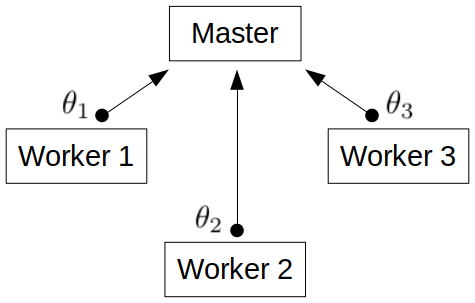
(a) “In”: workers send the samples drawn from the local posteriors to the master node.

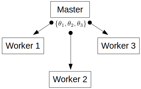
(b) “Out”: samples are pooled in the master node and broadcast to each of the workers.

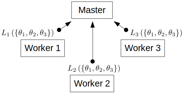
(c) “In”: workers compute likelihoods for the pooled samples using local data and send these to the master node.

Figure 1: The in-out-in algorithm of Section 2.2.1. This depicts an example where $M=3$ with data distributed across 3 workers and one master, which could be an edge node on a compute cluster. $\theta_{j}$ represents the set of samples drawn from the $j^{\textrm{{th}}}$ local posterior for $j=1,2,3$.

Figure 1 depicts the first 3 steps of this algorithm with a simple example in which $M=3$. Samples $\theta_{1},\theta_{2}$ and $\theta_{3}$ are drawn from each of three local posteriors. These are pooled in a master node and the pooled samples broadcast back to the workers. Then the workers compute the likelihoods $L_{1}\left(\left\{\theta_{1},\theta_{2},\theta_{3}\right\}\right),L_{2}\left(\left\{\theta_{1},\theta_{2},\theta_{3}\right\}\right)$ and $L_{3}\left(\left\{\theta_{1},\theta_{2},\theta_{3}\right\}\right)$ and send these back to the master. In this example, the master node does not hold any data or draw any samples. This could be an example of an edge node on a cluster consisting of itself and 3 compute nodes. Alternatively, the master node which pools samples and collects likelihoods could also play the role of a worker node, running its own MCMC sampler targeting the local posterior using local data.

2.2.2 Multiple importance estimator 1

Our first estimator takes a weighted average of local importance estimators. The weight to use for the $j^{\textrm{{th}}}$ local posterior is

$$q_{j}:=\frac{N_{j}}{N},$$ (13)

for $j=1,2,\ldots,M$, where $N=\sum_{j=1}^{M}N_{j}$. This is similar to the approach Veach and Guibas, (1995) called the “combined estimator”, but we use self-normalised importance weights Equation 9 where those authors assumed the densities involved were normalised. The estimator is

$$\tilde{\mu}^{\textrm{{MIE1}}}:=\sum_{j=1}^{M}\frac{N_{j}}{N}\sum_{h=1}^{N_{j}}\tilde{\mathbf{w}}_{j}\left(\theta_{j,h}\right)f\left(\theta_{j,h}\right).$$ (14)

That this is asymptotically unbiased follows from the single self-normalised importance estimator, Equation 10, being unbiased and

$$\mathbb{{E}}\left[\sum_{j=1}^{M}\frac{N_{j}}{N}\tilde{\mu}_{j}\right]=\mathbb{{E}}\left[\tilde{\mu}_{j}\right].$$ (15)

The variance of this estimator can be approximated as

$$\mathrm{{Var}}\left(\tilde{\mu}^{\textrm{{MIE1}}}\right)\approx\sum_{j=1}^{M}\frac{N_{j}}{N^{2}}\mathbb{{E}}_{\pi}\left[w_{j}\left(\theta\right)\left(f\left(\theta\right)-\mathbb{{E}}_{\pi}\left[f\left(\theta\right)\right]\right)^{2}\right],$$ (16)

which follows from

$$\mathrm{{Var}}\left(\tilde{\mu}^{\textrm{{MIE1}}}\right)=\sum_{j=1}^{M}\frac{N_{j}^{2}}{N^{2}}\mathrm{{Var}}\left(\tilde{\mu}_{j}\right)$$ (17)

and the approximate variance for self-normalised importance sampling (SNIS), $\mathrm{{Var}}\left(\tilde{\mu}_{j}\right)$, derived using the delta method for a ratio of means (see e.g. Owen, (2013)).

2.2.3 Multiple importance estimator 2

Importance sampling fails when the proposal p.d.f. and the target p.d.f. have little overlap; in particular, when regions of parameter space with high posterior density have low proposal density. In this case most sample weights will be close to zero and some rare samples will have very large weight, and consequently the estimator $\tilde{\mu}_{j}$ will have high variance. The risk of this increases as the dimension of the parameter space increases (MacKay et al., (2003)).

Our second estimator combines the local posteriors in a mixture distribution and uses this for the denominator of the importance weights. This reflects the intuition that the mixture of local posterior p.d.f.s is likely to provide better coverage of the posterior p.d.f., resulting in more stable sample weights. We define the mixture distribution with p.d.f.

$$\phi\left(\theta\right):=\sum_{j=1}^{M}q_{j}\pi_{j}\left(\theta\mid\mathbf{x}_{j}\right)$$ (18)

and component weights $q_{j}=\frac{N_{j}}{N}$ chosen so that the pooled samples from the local posteriors can be considered samples from $\phi$.

The use of a mixture distribution in importance sampling was investigated by Veach and Guibas, (1995) and named the “balance heuristic”. However, those authors assumed that all of the component distributions in the mixture had computable p.d.f.s. In other words, the normalising constants must be known to use the balance heuristic. The weights in the balance heuristic can be defined as

$$w_{\phi}\left(\theta\right):=\frac{\pi\left(\theta\mid x_{1:n}\right)}{\phi\left(\theta\right)}.$$ (19)

Then, as in Equation 7,

$$\mathbb{{E}}\left[w_{\phi}\left(\theta\right)f\left(\theta\right)\right]=\mathbb{{E}}_{\pi}\left[f\left(\theta\right)\right].$$ (20)

However, if the densities in Equation 19 were unnormalised, e.g.

$$\tilde{w}_{\phi}^{\textrm{{BH}}}\left(\theta\right):=\frac{\tilde{\pi}\left(\theta\mid x_{1:n}\right)}{\frac{1}{N}\sum_{j=1}^{M}N_{j}\tilde{\pi}_{j}\left(\theta\mid\mathbf{x}_{j}\right)},$$ (21)

the average

$$\frac{1}{N}\sum_{j=1}^{M}\sum_{h=1}^{N_{j}}\tilde{w}_{\phi}^{\textrm{{BH}}}\left(\theta_{j,h}\right)$$ (22)

would not be an unbiased estimator of the normalising constants as in Equation 11, and therefore the resulting estimator of $\mathbb{{E}}_{\pi}\left[f\left(\theta\right)\right]$ is biased, even with self-normalised weights and any number of samples.

Our MIE2 estimator fills this gap, i.e. it is an asymptotically unbiased estimator of $\mathbb{{E}}_{\pi}\left[f\left(\theta\right)\right]$ using a mixture of unnormalised densities. We will use a similar idea to Equation 11 where the weights provide a Monte Carlo estimate of the ratio of normalising constants. To this end, define

$$\hat{c}_{j}:=\frac{1}{N_{j}}\sum_{h=1}^{N_{j}}\tilde{w}_{j}\left(\theta_{j,h}\right)$$ (23)

for $j=1,2,\ldots,M$. Let

$$\tilde{\psi}\left(\theta\right):=\sum_{j=1}^{M}q_{j}\hat{c}_{j}\tilde{\pi}_{j}\left(\theta\mid\mathbf{x}_{j}\right)$$ (24)

and define the importance weights

$$\tilde{w}_{\phi}\left(\theta\right):=\frac{\tilde{\pi}\left(\theta\mid x_{1:n}\right)}{\tilde{\psi}\left(\theta\right)}$$ (25)

(we deliberately use the notation $\tilde{\psi}$ rather than $\tilde{\phi}$, despite the resemblance of $\tilde{\psi}$ to the mixture distribution $\phi$, to avoid misleading the reader into assuming that dividing $\tilde{\psi}$ by its integral with respect to $\theta$ results in $\phi$: it does not, as explained above in relation to why the balance heuristic does not work). Assume that $\tilde{\psi}\left(\theta\right)>0$ for all $\theta$ such that $\pi\left(\theta\mid x_{1:n}\right)>0$ (this is a weaker assumption than in MIE1 because only one of the local posterior densities needs to be positive for $\tilde{\psi}\left(\theta\right)>0$). Then we define the estimator

$$\tilde{\mu}^{\textrm{{MIE2}}}:=\frac{1}{N}\sum_{j=1}^{M}\sum_{h=1}^{N_{j}}\tilde{w}_{\phi}\left(\theta_{j,h}\right)f\left(\theta_{j,h}\right).$$ (26)

This is asymptotically unbiased, as shown in Appendix A.1.2; briefly, this is because $\tilde{w}_{\phi}\left(\theta\right)\to w_{\phi}\left(\theta\right)$ as all of the $N_{j}\to\infty$, with the $\hat{c}_{j}$ terms in Equation 24 in the limit supplying the normalising constants.

In practise we find that self-normalising the weights is beneficial to this estimator. Define the self-normalised importance weights

$$\tilde{\mathbf{w}}_{\phi}\left(\theta\right):=\frac{\tilde{w}_{\phi}\left(\theta\right)}{\sum_{j=1}^{M}\sum_{h=1}^{N_{j}}\tilde{w}_{\phi}\left(\theta_{j,h}\right)},$$ (27)

and the self-normalised estimator

$$\bar{\tilde{\mu}}^{\textrm{{MIE2}}}:=\sum_{j=1}^{M}\sum_{h=1}^{N_{j}}\tilde{\mathbf{w}}_{\phi}\left(\theta_{j,h}\right)f\left(\theta_{j,h}\right).$$ (28)

It can be shown (see Appendix A.2.1) that the finite sample bias of $\tilde{\mu}^{\textrm{{MIE2}}}$ is approximately

$$\mathbb{{E}}\left[\tilde{\mu}^{\textrm{{MIE2}}}\right]-\mathbb{{E}}_{\pi}\left[f\left(\theta\right)\right]\approx\frac{1}{\mathbb{{E}}\left[\phi\left(\theta\right)\right]^{2}}\textrm{{Var}}\left(\varepsilon\left(\theta\right)\right)\frac{\mathbb{{E}}\left[\pi\left(\theta\mid x_{1:n}\right)f\left(\theta\right)\right]}{\mathbb{{E}}\left[\phi\left(\theta\right)\right]},$$

where $\textrm{{Var}}\left(\varepsilon\left(\theta\right)\right)$, given by Equation 101 in Appendix A.2.1, is related to the Monte Carlo errors of the $\hat{c}_{j}$ estimators, which go to zero with $\sqrt{{N_{j}}}$. The variance of $\tilde{\mu}^{\textrm{{MIE2}}}$ can be approximated using a similar approach; see Appendix A.2.2. The variance of $\bar{\tilde{\mu}}^{\textrm{{MIE2}}}$ can be approximated using the delta method for the variance of SNIS (see e.g. Owen, (2013)).

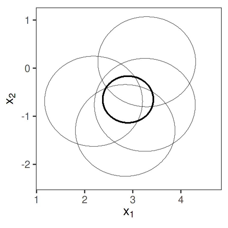
(a) Contours of the posterior and $M=4$ local posteriors (50 outcomes each).

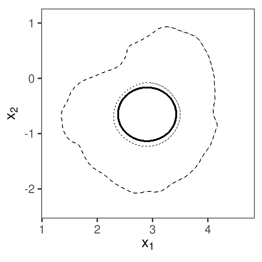
(b) Contours of the same posterior and of KDEs for the naive pooling method and MIE2.

Figure 2: Contours of the central 90% high density region of a 2 dimensional MVN posterior distribution, from $n=200$ simulated MVN outcomes, and an approximation using MIE2 from Section 2.2.3.

Figure 2 presents an example of how the MIE2 estimator approximates the posterior using samples from $M=4$ local posteriors. The data for this example are $n=200$ simulated 2 dimensional multivariate normal (MVN) outcomes with mean vector $\left[3.00,-0.72\right]^{\intercal}$ and covariance matrix $\left[12.06,10.22\right]I_{2}$ (we use $I_{p}$ for the identity matrix of dimension $p$). The estimand is the mean vector, with the covariance matrix known and using an uninformative MVN prior; see Section 3.2 for more details. Figure 2a depicts contours of the central 90% high density region of the posterior and local posteriors. Figure 2b depicts the central 90% for kernel density estimation (KDE) approximations to the posterior based on naive pooling of samples (“naive”) and the MIE2 estimator (Section 2.2.5 explains how to perform KDE with the MIE estimators). The MIE2 KDE approximates the posterior well, at least the greatest 90% of the density, and is certainly a much closer approximation than naive pooling.

2.2.4 Multiple importance estimator 3

The mixture distribution $\phi$ has component weights $\nicefrac{{N_{j}}}{{N}}$ because the importance estimator with proposal $\phi$ uses all of the samples available and a fraction $\nicefrac{{N_{j}}}{{N}}$ of them are drawn from the $j^{\textrm{{th}}}$ component. This is regardless of the utility of each component for constructing an approximation to the posterior: if the $j^{\textrm{{th}}}$ component is a good approximation to the posterior and the $k^{\textrm{{th}}}$ component is a poor one, MIE2 still uses all $N_{j}$ samples from the former and all $N_{k}$ samples from the latter.

One idea for a more efficient estimator is to relax the requirement that all components have the same weight and use the component weights to prioritise samples from some local posteriors over others. The drawback is we must compromise on using all samples available, discarding samples from those local posteriors with lower component weight.

We use the Kullback-Leibler (KL) divergence from the posterior to a local posterior to measure the ability of the latter to approximate the former. The KL divergence is defined as

$$D_{\mathrm{{KL}}}\left(q\parallel\pi\right):=H\left(q,\pi\right)-H\left(q\right)$$ (29)

with

$$H\left(q,\pi\right):=-\mathbb{{E}}_{q}\left[\log\left(\pi\left(\theta\right)\right)\right],$$ (30)

the cross entropy of target $\pi$ relative to an approximating distribution $q$, and

$$H\left(q\right):=-\mathbb{{E}}_{q}\left[\log\left(q\left(\theta\right)\right)\right],$$ (31)

the (differential) entropy of $q$. We use $D_{\mathrm{{KL}}}\left(\pi_{j}\parallel\pi\right)$ for the $j^{\textrm{{th}}}$ local posterior. $D_{\mathrm{{KL}}}\left(\pi_{j}\parallel\pi\right)$ is non-negative for all $\pi_{j}$ and $\pi$; when it is zero, the $j^{\textrm{{th}}}$ local posterior is equal to the posterior, which means if this component of the mixture is given component weight 1 all samples in the importance estimator will have a weight of 1. On the other hand, when $D_{\mathrm{{KL}}}\left(\pi_{j}\parallel\pi\right)$ is large there will be regions of $\theta$ where $\pi\left(\theta\right)\gg\pi_{j}\left(\theta\right)$, so if the $j^{\textrm{{th}}}$ local posterior has a relatively large component weight the resulting importance weights are likely to be degenerate. These observations suggest setting mixture component weights inversely proportional to $D_{\mathrm{{KL}}}\left(\pi_{j}\parallel\pi\right)$.

The KL divergence cannot be computed exactly because the normalising constants of the p.d.f.s involved are unknown. It can be estimated as

$$D_{\mathrm{{KL}}}\left(\pi_{j}\parallel\pi\right) = \mathbb{{E}}\left[\log\left(\frac{\tilde{\pi}_{j}\left(\theta\right)}{\tilde{\pi}\left(\theta\right)}\right)\right]+\log\left(\frac{Z_{\pi}}{Z_{j}}\right)$$ (32)

$$\approx -\frac{1}{N_{j}}\sum_{h=1}^{N_{j}}\log\tilde{w}_{j}\left(\theta_{j,h}\right)+\log\left(\frac{1}{N_{j}}\sum_{h=1}^{N_{j}}\tilde{w}_{j}\left(\theta_{j,h}\right)\right)$$

$$=:\widehat{D_{\mathrm{{KL}}}}\left(\pi_{j}\parallel\pi\right),$$

using Equations 3 and 11 with samples $\theta_{j,h}\sim\pi_{j}$. We then set $\tilde{q}_{j}:=\nicefrac{{1}}{{\widehat{D_{\mathrm{{KL}}}}\left(\pi_{j}\parallel\pi\right)}}$ for each $j$ and use mixture component weights

$$q_{j}:=\frac{\tilde{q}_{j}}{\sum_{i=1}^{M}\tilde{q}_{i}}$$ (33)

in Equation 18. Then we sample from the set $\left\{\theta_{j,h}:j=1,2,\ldots,M,h=1,2,\ldots,N_{j}\right\}$ $\min_{j}N_{j}$ times where each $\theta_{j,h}$ has probability of being sampled $\nicefrac{{q_{j}}}{{N_{j}}}$. This can also be achieved by first sampling an index $j\in\left\{1,2,\ldots,M\right\}$ $\bar{N}:=\min_{j}N_{j}$ times where the probability of sampling $j$ is $q_{j}$, then for each sampled $j$ draw a sample from $\left\{\theta_{j,h};h=1,2,\ldots,N_{j}\right\}$ uniformly at random. Denote the resulting sample $\tilde{\theta}_{h},h=1,2,\ldots,\bar{N}$. We compute importance weights for this sample using Equation 25, using the original $\hat{c}_{j}$ estimates in Equation 24, and define the estimator

$$\tilde{\mu}^{\textrm{{MIE3}}}:=\frac{1}{\bar{N}}\sum_{h=1}^{\bar{N}}\tilde{w}_{\phi}\left(\tilde{\theta}_{h}\right)f\left(\tilde{\theta}_{h}\right).$$ (34)

As with $\bar{\tilde{\mu}}^{\textrm{{MIE2}}}$, this benefits from the weights being normalised, so in practise we prefer to use

$$\bar{\tilde{\mu}}^{\textrm{{MIE3}}}:=\sum_{h=1}^{\bar{N}}\tilde{\mathbf{w}}_{\phi}\left(\tilde{\theta}_{h}\right)f\left(\tilde{\theta}_{h}\right)$$ (35)

with $\tilde{\mathbf{w}}_{\phi}$ from Equation 27. The finite sample bias and variance of $\tilde{\mu}^{\textrm{{MIE3}}}$ are the same as for $\tilde{\mu}^{\textrm{{MIE2}}}$ but with denominator $\bar{N}$ instead of $N$.

2.2.5 Density estimation with MIE

The posterior density $\pi\left(\theta^{\prime}\mid x_{1:n}\right)$ can be estimated using $\tilde{\mu}^{\textrm{{MIE1}}},\bar{\tilde{\mu}}^{\textrm{{MIE2}}}$ or $\bar{\tilde{\mu}}^{\textrm{{MIE3}}}$. For example, using a rectangular window kernel, this would be, for MIE2:

$$\bar{\tilde{\mu}}^{\textrm{{MIE2}}}\left(K_{\xi}\left(\theta,\theta^{\prime}\right)\right)=\frac{1}{\xi}\sum_{j=1}^{M}\sum_{h=1}^{N}\tilde{\mathbf{w}}_{\phi}\left(\theta_{j,h}\right)\mathbf{{1}}\left(\left|\theta_{j,h}-\theta^{\prime}\right|<\frac{\xi}{2}\right),$$ (36)

where $\mathbf{{1}}\left(P\right)=1$ if $P$ is true and is zero otherwise.

2.3 Additional samples from Laplace approximations

We propose an extension to the estimators described in Section 2.2 which may improve their utility in applications where they may struggle, such as with large dimension $p$. Our idea is to supplement the samples from the local posteriors with additional samples drawn from one of three Laplace approximations to the posterior constructed from the local posteriors. The intention is that the importance estimators can be improved by providing better representation of regions of $\theta$ under the posterior where little is provided by the local posteriors.

A Laplace approximation is an MVN with mean and covariance matrix chosen to approximate a posterior distribution. With such an approximation we can generate any number of samples much faster, in general, than generating additional samples from the local posteriors (which may require many likelihood evaluations).

Samples from a Laplace approximation can be included in the MIE 1, 2 or 3 estimators as an additional importance proposal or mixture component. We will sample $N_{M+j}$ samples from Laplace approximation $j=1,2,3$. To enrich MIE1, we define importance weights

$$\tilde{w}_{M+j}\left(\theta\right):=\frac{\tilde{\pi}\left(\theta\mid x_{1:n}\right)}{\varphi\left(\theta;\mu_{j}^{\textrm{{La}}},\Sigma_{j}^{\textrm{{La}}}\right)}$$ (37)

for $j=1,2,3$, where $\varphi\left(\theta;\mu_{j}^{\textrm{{La}}},\Sigma_{j}^{\textrm{{La}}}\right)$ is the p.d.f. of the Laplace approximation MVN with mean $\mu_{j}^{\textrm{{La}}}$ and covariance matrix $\Sigma_{j}^{\textrm{{La}}}$ (which will be defined later in this section). Then, with Laplace samples

$$\theta_{M+j,h}\sim\mathrm{{N}}_{p}\left(\mu_{j}^{\textrm{{La}}},\Sigma_{j}^{\textrm{{La}}}\right),j=1,2,3,h=1,2,\ldots,N_{M+j},$$

the LEMIE1 estimator is

$$\tilde{\mu}^{\textrm{{LEMIE1}}}:=\sum_{j=1}^{M+3}\frac{N_{j}}{N^{\textrm{{La}}}}\sum_{h=1}^{N_{j}}\tilde{\mathbf{w}}_{j}\left(\theta_{j,h}\right)f\left(\theta_{j,h}\right),$$ (38)

where $N^{\textrm{{La}}}:=\sum_{j=1}^{M+3}N_{j}$. For LEMIE2, we can include Laplace samples in the mixture distribution approximation Equation 24 thus:

$$\tilde{\psi}^{\textrm{{La}}}\left(\theta\right):=\sum_{j=1}^{M}q_{j}\hat{c}_{j}\tilde{\pi}_{j}\left(\theta\mid\mathbf{x}_{j}\right)+\sum_{j=1}^{3}q_{M+j}\hat{c}_{M+j}\varphi\left(\theta;\mu_{j}^{\textrm{{La}}},\Sigma_{j}^{\textrm{{La}}}\right),$$ (39)

where the component weights are now $q_{j}=\frac{N_{j}}{N^{\textrm{{La}}}}$ for $j=1,2,\ldots,M+3$. Then we use

$$\tilde{w}_{\phi}^{\textrm{{La}}}\left(\theta\right):=\frac{\tilde{\pi}\left(\theta\mid x_{1:n}\right)}{\tilde{\psi}^{\textrm{{La}}}\left(\theta\right)},$$ (40)

$$\tilde{\mathbf{w}}_{\phi}^{\textrm{{La}}}\left(\theta\right):=\frac{\tilde{w}_{\phi}^{\textrm{{La}}}\left(\theta\right)}{\sum_{j=1}^{M+3}\sum_{h=1}^{N_{j}}\tilde{w}_{\phi}^{\textrm{{La}}}\left(\theta_{j,h}\right)},$$ (41)

and the resulting self-normalised estimator is

$$\bar{\tilde{\mu}}^{\textrm{{LEMIE2}}}:=\sum_{j=1}^{M+3}\sum_{h=1}^{N_{j}}\tilde{\mathbf{w}}_{\phi}^{\textrm{{La}}}\left(\theta_{j,h}\right)f\left(\theta_{j,h}\right).$$ (42)

The LEMIE3 estimator is similar except the component weights are

$$q_{j}:=\frac{\tilde{q}_{j}}{\sum_{i=1}^{M+3}\tilde{q}_{i}},$$ (43)

for $j=1,2,\ldots,M+3$, in place of Equation 33 with

$$\tilde{q}_{M+j}:=\frac{1}{\widehat{D_{\mathrm{{KL}}}}\left(\varphi_{j}\parallel\pi\right)}$$ (44)

for $j=1,2,3$ and in which $\varphi_{j}$ is the density function of the $j^{\textrm{{th}}}$ Laplace approximation. Then samples are resampled from the $M+3$ components with probabilities $q_{j}$ as in Section 2.2.4. The estimator $\widehat{D_{\mathrm{{KL}}}}\left(\varphi_{j}\parallel\pi\right)$ in this case can be made more efficient than Equation 32 because $H\left(\varphi_{j}\right)=\frac{1}{2}\log\det\left(2\pi e\Sigma_{j}^{\textrm{{La}}}\right)$ (Cover and Thomas, (2006)), so only the cross entropy in Equation 29 needs to be estimated.

The three ways to construct a Laplace approximation from the local posterior samples are as follows.

2.3.1 Laplace approximation 1: parametric estimator

If we assume the local posteriors are MVN with mean $\mu_{j}$ and covariance matrix $\Sigma_{j}$ for the $j^{\textrm{{th}}}$ local posterior then the linear combination

$$\left(\sum_{j=1}^{M}\Sigma_{j}^{-1}\right)^{-1}\left(\sum_{j=1}^{M}\Sigma_{j}^{-1}\theta_{j,h}\right)$$ (45)

also follows an MVN. Under an additional assumption, this MVN is also the posterior: this is the motivation for the consensus Monte Carlo algorithm of Scott et al., (2016) and the parametric density product estimator (PDPE) of Neiswanger et al., (2013) (see Section 2.5.1 for more details). We define

$$\Sigma_{1}^{\textrm{{La}}}:=\left(\sum_{j=1}^{M}\hat{\Sigma}_{j}^{-1}\right)^{-1}$$ (46)

and

$$\mu_{1}^{\textrm{{La}}}:=\Sigma_{1}^{\textrm{{La}}}\left(\sum_{j=1}^{M}\hat{\Sigma}_{j}^{-1}\hat{\mu}_{j}\right),$$ (47)

where $\hat{\mu}_{j}$ and $\hat{\Sigma}_{j}$ are respectively the sample mean and sample covariance matrix for the $j^{\textrm{{th}}}$ local posterior, and

$$\bar{\theta}_{h}:=\Sigma_{1}^{\textrm{{La}}}\left(\sum_{j=1}^{M}\hat{\Sigma}_{j}^{-1}\theta_{j,h}\right),$$ (48)

which is distributed as $\mathrm{{N}}_{p}\left(\mu_{1}^{\textrm{{La}}},\Sigma_{1}^{\textrm{{La}}}\right)$ if the local posteriors are MVN. This is our first Laplace approximation. We can pool up to $\bar{N}$ samples using Equation 48 for use in the LEMIE estimators. Additional samples can be generated from $\mathrm{{N}}_{p}\left(\mu_{1}^{\textrm{{La}}},\Sigma_{1}^{\textrm{{La}}}\right)$ if required.

Numerical problems can arise in the calculation of the $\hat{\Sigma}_{j}^{-1}$, particularly when $p$ is large. When $\hat{\Sigma}_{j}$ cannot be inverted we fall back to using the diagonal matrix with the variances in $\hat{\Sigma}_{j}$ on the diagonal, following Scott et al., (2016).

2.3.2 Laplace approximation 2: pooled estimated Laplace

Our second idea is to use the maximum likelihood estimates of the mean and covariance matrix of an MVN for all the pooled samples from the local posteriors. These are the sample mean and sample covariance matrix. I.e.

$$\mu_{2}^{\textrm{{La}}}:=\frac{1}{N}\sum_{j=1}^{M}\sum_{h=1}^{N_{j}}\theta_{j,h},$$ (49)

$$\Sigma_{2}^{\textrm{{La}}}:=\frac{1}{N-1}\sum_{j=1}^{M}\sum_{h=1}^{N_{j}}\left(\theta_{j,h}-\mu_{2}^{\textrm{{La}}}\right)\left(\theta_{j,h}-\mu_{2}^{\textrm{{La}}}\right)^{\intercal},$$ (50)

and any number of samples can be drawn from $\mathrm{{N}}_{p}\left(\mu_{2}^{\textrm{{La}}},\Sigma_{2}^{\textrm{{La}}}\right)$. This approximation is likely to be relatively diffuse, which may help when local posterior coverage of the posterior p.d.f. is very poor.

2.3.3 Laplace approximation 3: Bayesian estimated Laplace

Our third idea is to pool all the samples as above but then to place an inverse Wishart prior on their covariance matrix,

$$\Sigma\sim\mathrm{{IW}}\left(\Psi^{\textrm{{La3}}},\nu^{\textrm{{La3}}}\right),$$ (51)

with scale matrix $\Psi^{\textrm{{La3}}}$ and degrees of freedom $\nu^{\textrm{{La3}}}$, and compute the posterior mean of $\Sigma$ using the samples as data after shifting them to have mean zero. That is,

$$\Sigma_{3}^{\textrm{{La}}}:=\frac{1}{N+\nu^{\textrm{{La3}}}-p-1}\left(\sum_{j=1}^{M}\sum_{h=1}^{N_{j}}\left(\theta_{j,h}-\hat{\theta}_{j}\right)\left(\theta_{j,h}-\hat{\theta}_{j}\right)^{\intercal}+\Psi^{\textrm{{La3}}}\right),$$

where $\hat{\theta}_{j}:=\frac{1}{N_{j}}\sum_{h=1}^{N_{j}}\theta_{j,h}$ for each $j$. Then set the mean vector $\mu_{3}^{\textrm{{La}}}$ to be the pooled sample mean Equation 49, and any number of samples can be drawn from $\mathrm{{N}}_{p}\left(\mu_{3}^{\textrm{{La}}},\Sigma_{3}^{\textrm{{La}}}\right)$. This approximation is similar to that in Section 2.3.2, but we have some influence over its shape, in particular how diffuse it is, via the prior parameters $\Psi^{\textrm{{La3}}}$ and $\nu^{\textrm{{La3}}}$.

2.4 Estimator diagnostics

2.4.1 Effective sample size

The effective sample size (ESS) of a Monte Carlo estimator, in the definition of Kong, (1992), is the ratio of the posterior variance of the estimand to the variance of the estimator, which measures the efficiency lost due to sampling from the approximation rather than the posterior itself.

We can derive an estimate of the ESS for each of the estimators in Section 2.2 with an additional application of the delta method to the variance estimates. These are, for MIE 1, 2 and 3 respectively:

$$\textrm{{ESS}}_{1}\approx\frac{1}{\sum_{j=1}^{M}\frac{N_{j}^{2}}{N^{2}}\sum_{h=1}^{N_{j}}\tilde{\mathbf{w}}_{j}\left(\theta_{j,h}\right)^{2}},$$ (52)

$$\textrm{{ESS}}_{2}\approx\frac{1}{\sum_{j=1}^{M}\sum_{h=1}^{N_{j}}\tilde{\mathbf{w}}_{\phi}\left(\theta_{j,h}\right)^{2}},$$ (53)

and

$$\textrm{{ESS}}_{3}\approx\frac{1}{\sum_{h=1}^{\bar{N}}\tilde{\mathbf{w}}_{\phi}\left(\tilde{\theta}_{h}\right)^{2}}.$$ (54)

When Laplace samples are included these become

$$\textrm{{ESS}}_{1}^{\textrm{{La}}}\approx\frac{1}{\sum_{j=1}^{M+3}\frac{N_{j}^{2}}{N^{2}}\sum_{h=1}^{N_{j}}\tilde{\mathbf{w}}_{j}\left(\theta_{j,h}\right)^{2}},$$ (55)

$$\textrm{{ESS}}_{2}^{\textrm{{La}}}\approx\frac{1}{\sum_{j=1}^{M+3}\sum_{h=1}^{N_{j}}\tilde{\mathbf{w}}_{\phi}^{\textrm{{La}}}\left(\theta_{j,h}\right)^{2}},$$ (56)

and

$$\textrm{{ESS}}_{3}^{\textrm{{La}}}\approx\frac{1}{\sum_{h=1}^{\bar{N}}\tilde{\mathbf{w}}_{\phi}^{\textrm{{La}}}\left(\tilde{\theta}_{h}\right)^{2}}.$$ (57)

A derivation of Equation 52 can be found in Appendix A.3. Equations 53 and 54 for MIE2 and MIE3 respectively are equivalent to the approximate ESS for SNIS; see e.g. Owen, (2013) and the derivation of Kong, (1992).

2.4.2 Tail distribution shape estimate ($\hat{{k}}$)

Vehtari et al., (2015) introduce a useful diagnostic for importance sampling, introduced as part of an algorithm to smooth importance weights. This is used by Vehtari et al., (2017) for leave-one-out cross validation (LOO). Their LOO estimator is computed using importance sampling with the weights smoothed to make them more stable and improve the estimator’s accuracy and reliability. Importance weights have a tail distribution that is, in the limit, well-approximated by a generalised Pareto distribution (GPD) under weak conditions (Pickands III, (1975)). The idea of Vehtari et al., (2015) is to replace the largest weights above a threshold with quantiles from the fitted GPD.

The GPD has shape parameter $k\in\mathbb{{R}}$, which is estimated as $\hat{{k}}$ using the efficient estimator of Zhang and Stephens, (2009) (along with the other parameters). Vehtari et al., (2015) find empirically that $\hat{{k}}$ is a useful diagnostic, indicating when an importance estimator may be unreliable. They find that $\hat{{k}}<0.5$ is an indicator of good performance, but that Pareto smoothed importance weights will still provide reliable results for $\hat{{k}}<0.7$ and that importance sampling is unreliable beyond this. The R package loo (Vehtari et al., (2022)) includes an implementation of the $\hat{{k}}$ estimator.

2.5 Other approaches

In this section we briefly describe the estimators of Scott et al., (2016) and Neiswanger et al., (2013), which are used for comparisons with our methods in Section 3. Each of these approaches starts from the observation that

$$\pi\left(\theta\mid x_{1:n}\right)\propto\prod_{j=1}^{M}p\left(\mathbf{x}_{j}\mid\theta\right)\pi\left(\theta\right)^{\nicefrac{{1}}{{M}}},$$ (58)

assuming $\mathbf{x}_{j}$ is conditionally independent of $\mathbf{x}_{k}$, for all $j\neq k$, given $\theta$. I.e. the posterior p.d.f. is a product of the local posterior p.d.f.s using the prior with density $\pi\left(\theta\right)^{\nicefrac{{1}}{{M}}}$, which is referred to as the fractionated prior.

2.5.1 Consensus Monte Carlo

As explained in Section 2.3.1, if $\mu_{j}$ and $\Sigma_{j}$ are the mean and covariance matrix of the $j^{\textrm{{th}}}$ local posterior, and if the posterior and local posteriors are MVN, then linear combinations of samples Equation 45 also follow an MVN. If the prior used in the local posteriors has density $\pi\left(\theta\right)^{\nicefrac{{1}}{{M}}}$ then that MVN is in fact the posterior. This can be seen from Equation 58 by inductively applying Bayes’ theorem with a normal likelihood function and a normal prior.

In the consensus Monte Carlo algorithm (CMC) of Scott et al., (2016) we define

$$\Sigma^{*}:=\left(\sum_{j=1}^{M}\tilde{\Sigma}_{j}^{-1}\right)^{-1}$$ (59)

and

$$\mu^{*}:=\Sigma^{*}\left(\sum_{j=1}^{M}\tilde{\Sigma}_{j}^{-1}\tilde{\mu}_{j}\right),$$ (60)

where $\tilde{\mu}_{j}$ and $\tilde{\Sigma}_{j}$ are respectively the sample mean and sample covariance matrix for the $j^{\textrm{{th}}}$ local posterior using the fractionated prior, and

$$\theta_{h}^{*}:=\Sigma^{*}\left(\sum_{j=1}^{M}\tilde{\Sigma}_{j}^{-1}\theta_{j,h}\right)$$ (61)

for $h=1,2,\ldots,\bar{N}$. When the posterior is not MVN, Monte Carlo estimators based on these samples should still be useful, especially in big data situations, because of the Bernstein-von Mises theorem (posterior distributions tend towards a normal distribution as $n\to\infty$, Van der Vaart, (1998)). Equation 61 requires the number of samples from each local posterior to be $\bar{N}$; samples from a local posterior in excess of this must be discarded.

There are two estimators defined by the choice of weight matrix in Equation 61. The first is

$$\tilde{\mu}^{\textrm{{CMC1}}}:=\frac{1}{\bar{N}}\sum_{h=1}^{\bar{N}}f\left(\frac{1}{M}\sum_{j=1}^{M}\theta_{j,h}\right),$$ (62)

i.e. the identity matrix $I_{p}$ is used for each of the weight matrices. The second estimator is

$$\tilde{\mu}^{\textrm{{CMC2}}}:=\frac{1}{\bar{N}}\sum_{h=1}^{\bar{N}}f\left(\Sigma^{*}\left(\sum_{j=1}^{M}\tilde{\Sigma}_{j}^{-1}\theta_{j,h}\right)\right).$$ (63)

When the posterior distribution is normal, $\tilde{\mu}^{\textrm{{CMC2}}}$ is an unbiased estimator of the posterior expectation of $f$. One drawback is that the method is unlikely to perform well when the posterior deviates greatly from normality. Another is that we must use the fractionated prior for the local posterior sampling. This can be a problem if the distribution with density $\pi\left(\theta\right)^{\nicefrac{{1}}{{M}}}$ is improper, in which case we may need to compromise on the form or parameterisation of the prior distribution. As in Section 2.3.1, numerical problems can arise in the calculation of the $\tilde{\Sigma}_{j}^{-1}$; here as well we fall back to using the diagonal matrix with the variances in $\hat{\Sigma}_{j}$ on the diagonal when $\hat{\Sigma}_{j}$ cannot be inverted.

There is a small sample bias correction proposed by Scott et al., (2016). We do not include this in our comparisons in Section 3 because we find the performance to be similar to that of the CMC2 algorithm without it.

2.5.2 Density product estimator

The density product

$$\pi_{1}\cdots\pi_{M}\left(\theta\right):=\prod_{j=1}^{M}\pi_{j}\left(\theta\mid\mathbf{x}_{j}\right),$$ (64)

with $\pi_{j}\left(\theta\mid\mathbf{x}_{j}\right)$ using the fractionated prior, is not necessarily equal to the posterior density but is proportional to it. Neiswanger et al., (2013) use kernel density estimation to approximate Equation 64 using the pooled samples from the local posteriors.The nonparametric density product estimator (NDPE) is designed to be more robust than CMC to deviations in the posterior from normality (they also propose a “parametric subposterior density product estimator”, PDPE, which is very similar to CMC so we have not included it). It uses a MVN KDE $\widehat{\pi_{1}\cdots\pi_{M}}$ that is asymptotically unbiased and consistent. The KDE for the $j^{\textrm{{th}}}$ local posterior, assuming all $N_{j}=\bar{N}$, as a function of $\theta$ is

$$\frac{1}{\bar{N}}\sum_{h=1}^{\bar{N}}\mathrm{{N}}_{p}\left(\theta\mid\theta_{j,h},b^{2}I_{p}\right),$$ (65)

where $b$ is a tuning parameter (bandwidth). The product of KDEs can be rewritten as a normal mixture density thus:

$$\hat{\pi}^{\mathrm{{NDPE}}}\left(\theta\right) := \frac{1}{\bar{N}^{M}}\prod_{j=1}^{M}\sum_{h=1}^{\bar{N}}\mathrm{{N}}_{p}\left(\theta\mid\theta_{j,h},b^{2}I_{p}\right)$$

$$\propto \sum_{h_{1}=1}^{\bar{N}}\cdots\sum_{h_{M}=1}^{\bar{N}}w\left(h_{1},\ldots,h_{M}\right)\mathrm{{N}}_{p}\left(\theta\mid\bar{\theta}\left(h_{1},\ldots,h_{M}\right),b^{2}I_{p}\right),$$

where

$$\bar{\theta}\left(h_{1},\ldots,h_{M}\right):=\frac{1}{M}\sum_{j=1}^{M}\theta_{j,h_{j}}$$ (67)

and with unnormalised component weights

$$w\left(h_{1},\ldots,h_{M}\right):=\prod_{j=1}^{M}\mathrm{{N}}_{p}\left(\theta_{j,h_{j}}\mid\bar{\theta}\left(h_{1},\ldots,h_{M}\right),b^{2}I_{p}\right).$$ (68)

There are $\bar{N}^{M}$ terms in the mixture density Equation LABEL:eq:ndpe, so it is not feasible to compute it exactly. Therefore, Neiswanger et al., (2013) propose to sample from it using an independent Metropolis-within-Gibbs algorithm which alternates between sampling $\theta$ from the mixture distribution given indices $h_{1},\ldots,h_{M}$ and sampling the indices independently of $\theta$ over $\bar{N}$ iterations. The resulting samples of $\theta$ can be used in Monte Carlo estimators of posterior expectations. The bias and variance of the method shrink as bandwidth $b\to 0$, so we set $b$ to $i^{\nicefrac{{-1}}{{p+4}}}$ in iteration $i$. This introduces an element of tempering.

The semiparametric density product estimator (SDPE) aims to combine the PDPE’s fast convergence with NDPE’s asymptotic properties. SDPE involves a KDE of $\frac{\pi_{j}\left(\theta\mid\mathbf{x}_{j}\right)}{\tilde{\varphi}_{j}\left(\theta\right)}$, the “correction function” of the normal approximation to the $j^{\textrm{{th}}}$ local posterior, where $\tilde{\varphi}_{j}$ is the density function of an MVN with parameters $\tilde{\mu}_{j}$ and $\tilde{\Sigma}_{j}$ from Section 2.5.1. The remaining details are similar to the NDPE algorithm; see Appendix B for details.

The MCMC samplers in NDPE and SDPE can suffer from slow mixing due to a low acceptance rate. Neiswanger et al., (2013) propose the sampler be applied separately to subsets of the local posteriors (e.g., pairwise), generating a new set of samples, then applied recursively to the output.

NDPE and SDPE can result in samples that are not possible values of the random variable $\theta$. For example, if $\theta$ is modelled to take only positive values, the DPE algorithms can generate pooled samples of $\theta$ that are negative. This means the algorithm will be biased near such boundaries, and in practise, it may be necessary to constrain the result of the algorithm to obtain valid results. In SDPE, as in CMC and Section 2.3.1, we must calculate $\tilde{\Sigma}_{j}^{-1}$ and so problems can also arise here when $\tilde{\Sigma}_{j}$ cannot be inverted, in which case we use the diagonal matrix with the variances in $\tilde{\Sigma}_{j}$ on the diagonal.

2.5.3 Naive pooling

In our experiments in Section 3 we will also compare the performance of the LEMIE estimators against the naive pooling estimator introduced in Section 2.1. This is the pooled sample average

$$\tilde{\mu}^{\textrm{{Naive}}}:=\frac{1}{N}\sum_{j=1}^{M}\sum_{h=1}^{N_{j}}f\left(\theta_{j,h}\right).$$ (69)

3 Simulation studies

This section presents results from experiments using synthetic data generated from three models: a beta-Bernoulli model for binary data, MVN data with normal-inverse Wishart priors for the mean and covariance matrix, and logistic regression with an MVN prior. The purpose of these studies is to explore differences in performance between the methods described in Section 2. Where possible, we also compare them against the $M=1$ case (i.e. using all data together on one node).

Each of our analyses was performed in R (R Core Team, (2020)), version 3.6.3. Most computation was carried out on a personal computer running a Linux operating system with an 8 core CPU and 16 GB RAM. Some were carried out on Amazon Web Services (AWS) Elastic Compute 2 (EC2) instances (Amazon Web Services, Inc., (2017)) with specifications (CPU cores / RAM): 8 / 16GB, 16 / 32GB, 32 / 64GB, 64 / 128GB.

In comparisons of point-wise estimation error, we use error function

$$E\left(f,\hat{f}\right):=\left\|\hat{f}-f\right\|_{2},$$ (70)

where $\left\|\cdot\right\|_{2}$ is the Euclidean 2-norm and $f,\hat{f}\in\mathbb{{R}}^{p}$. This will be used, for example, in comparing estimators of a posterior mean. Another measure of performance we use is the KL divergence between the posterior and the approximating distribution implied by each estimator.

KL divergence estimation

We define the cross entropy of an approximating distribution $q$ relative to target $\pi$

$$H\left(\pi,q\right):=-\mathbb{{E}}_{\pi}\left[\log\left(q\left(\theta\right)\right)\right].$$ (71)

In our simulations we are readily able to generate samples from the posterior, so this form is preferred over Equation 30 since using Equation 3 we can estimate Equation 71 as

$$H\left(\pi,q\right)\approx-\frac{1}{N^{*}}\sum_{h=1}^{N^{*}}\log\left(q\left(\theta_{h}\right)\right)$$ (72)

using samples $\theta_{h}\sim\pi,h=1,2,\ldots,N^{*}$. The standard error of this estimator can be estimated using the sample standard deviation of $\log\left(q\left(\theta_{h}\right)\right)$ divided by $\sqrt{{N^{*}}}$.

This definition of cross entropy features in the KL divergence from $q$ to $\pi$,

$$D_{\mathrm{{KL}}}\left(\pi\parallel q\right)=H\left(\pi,q\right)-H\left(\pi\right),$$ (73)

in which $H\left(\pi\right):=-\mathbb{{E}}_{\pi}\left[\log\left(\pi\left(\theta\right)\right)\right]$ is the entropy of $\pi$. Equation 72 is useful on its own for comparing the methods, but the fact that $D_{\mathrm{{KL}}}\left(\pi\parallel q\right)\geq 0$ allows us to assess performance on an absolute scale using Equation 73. In some simple models, an analytic form is known for $H\left(\pi\right)$, and in others samples from $\pi$ can be used to estimate it, again using Equation 3.

Density function $q$ can be estimated using kernel density estimation, either using the method described in Section 2.2.5 for LEMIE or using standard KDE with the pooled samples from the CMC, DPE or Naive methods. We use a normal kernel function; for LEMIE this means an MVN p.d.f. is used for $K_{\xi}\left(\theta,\theta^{\prime}\right)$ in Section 2.2.5 with $\xi$ being the smoothing covariance matrix.

3.1 Beta-Bernoulli model

We reproduce the example of Scott et al., (2016) in which $M=100$, data $x_{1:n}$ are binary with $n=1,000$ and exactly one of the outcomes are positive, say $x_{1}=1$, with the remainder being zero. The model is

$$x_{i}\sim\textrm{{Bernoulli}}\left(\lambda\right),i=1,2,\ldots,n,$$ (74)

and the estimand is the parameter $\lambda\in\left(0,1\right)$. We use a prior distribution of the form $\mathrm{{Beta}}\left(\beta_{1},\beta_{2}\right)$. This is a conjugate prior, and the posterior distribution is $\mathrm{{Beta}}\left(\beta_{1}+\sum_{i=1}^{n}x_{i},\beta_{2}+n-\sum_{i=1}^{n}x_{i}\right)$. Following Scott et al., (2016), we use $\beta_{1}=\beta_{2}=1$, which is equivalent to a uniform prior on $\left(0,1\right)$.

For CMC and DPE, following the principle of Equation 58 requires $\mathrm{{Beta}}\left(1,1\right)$ also be used as the fractionated prior. CMC does not perform well with that prior in this example, as demonstrated by Scott et al., (2016). The fractionated prior recommended for this example by Scott et al., (2016) is $\mathrm{{Beta}}\left(0.01,0.01\right)$ with the justification that using $\mathrm{{Beta}}\left(1,1\right)$ implies an additional “prior success”, which is too informative given the data only contain a single success. In fact it is the $\mathrm{{Beta}}\left(0.01,0.01\right)$ that is more informative; $\mathrm{{Beta}}\left(1,1\right)$ is the beta distribution of maximum differential entropy and in $\mathrm{{Beta}}\left(0.01,0.01\right)$ the density is concentrated close to 0 and 1.

We drew $\bar{N}=10,000$ samples from each local posterior, using each of the two priors: $\mathrm{{Beta}}\left(1,1\right)$, which is used by the MIE algorithms, and $\mathrm{{Beta}}\left(0.01,0.01\right)$, the fractionated prior proposed by Scott et al., (2016) and used by the CMC and DPE algorithms.

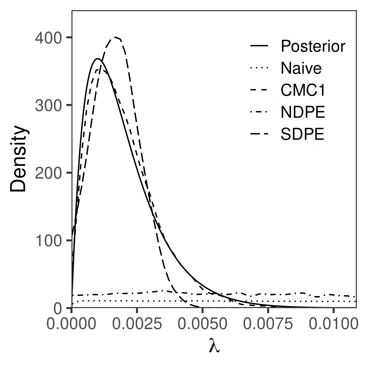
(a) KDE approximations for Naive, CMC1, NDPE and SDPE from Section 2.5.

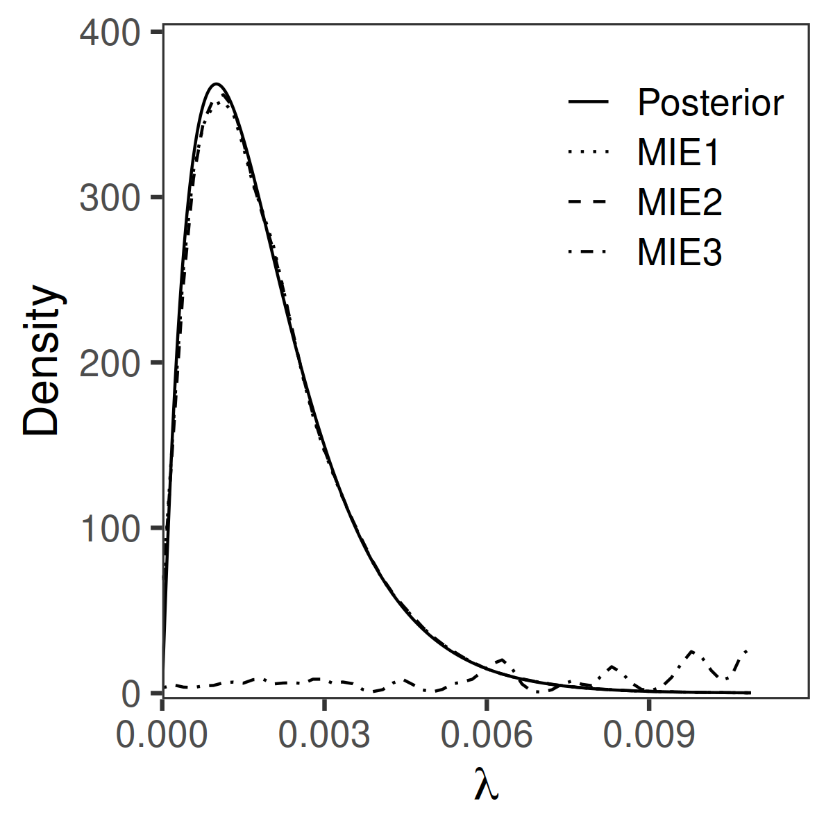
(b) KDE approximations for the MIE algorithms from Section 2.2.

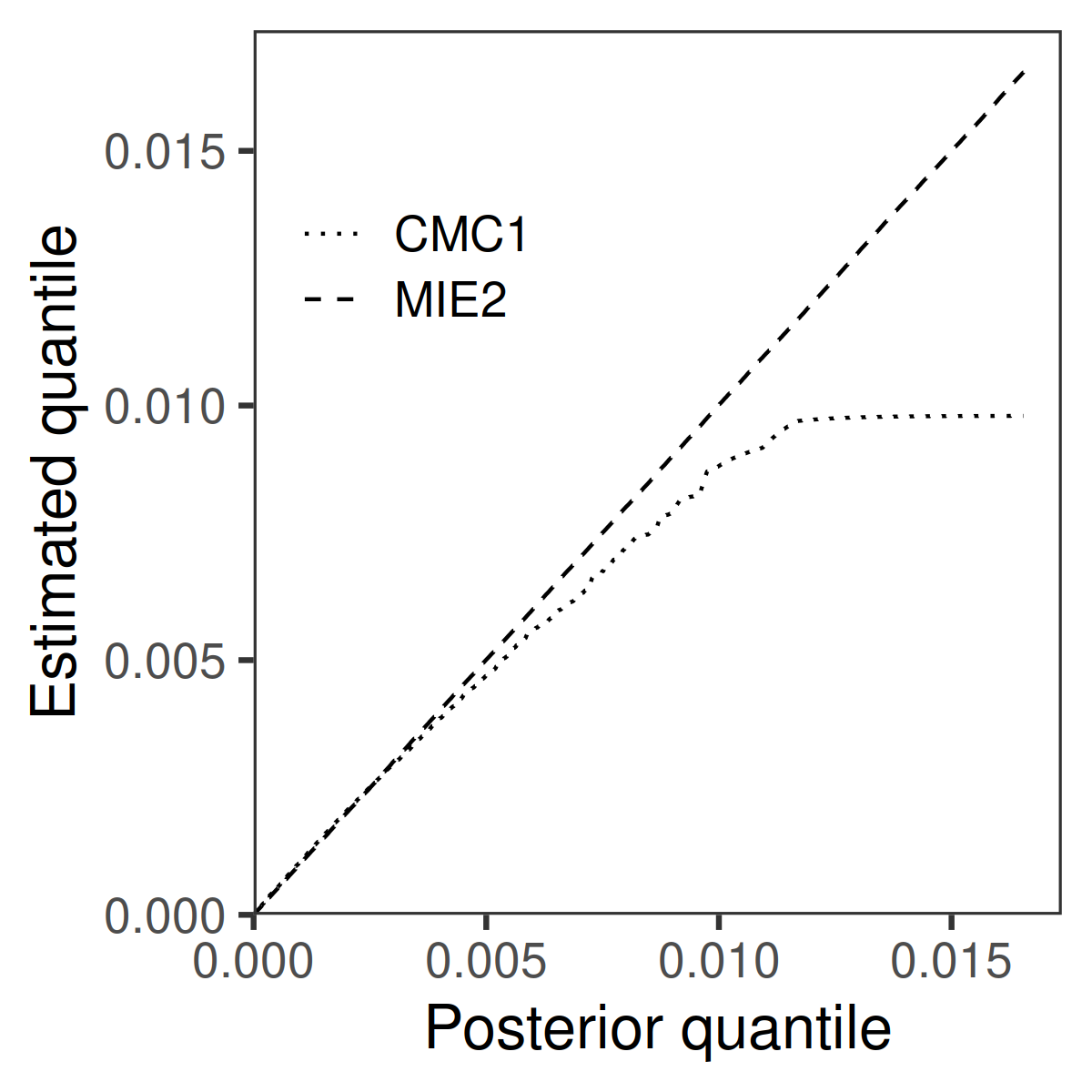
(c) Posterior quantile-quantile plot for the best of the estimators in (a) and (b).

Figure 3: KDE (bin width 0.000184) approximations of the beta posterior distribution in the example of Section 3.1 with one positive outcome ($n=1,000$).

Figure 3 presents the results of posterior density estimation in this example. As observed by Scott et al., (2016), the CMC1 algorithm using fractionated prior $\mathrm{{Beta}}\left(0.01,0.01\right)$ approximates the posterior p.d.f. quite well. We found that CMC2 is poor in this example (results not shown), even with the bias correction. The DPE algorithms perform less well, although better than naive pooling. MIE1 and MIE2 perform the best, as can be seen for MIE2 in the quantile-quantile plot of Figure 3c, with excellent approximation of the tail.

To investigate the role of the prior we looked at another example in which $\frac{n}{2}$ of the observations are positive and the remaining $\frac{n}{2}$ are zero, the likelihood of which would be maximised by $\lambda=\frac{1}{2}$, and we partition the data such that 50 of the $M=100$ parts contain positive outcomes only and the remaining 50 contain negative outcomes only. We used the same $\mathrm{{Beta}}\left(1,1\right)$ and $\mathrm{{Beta}}\left(0.01,0.01\right)$ priors.

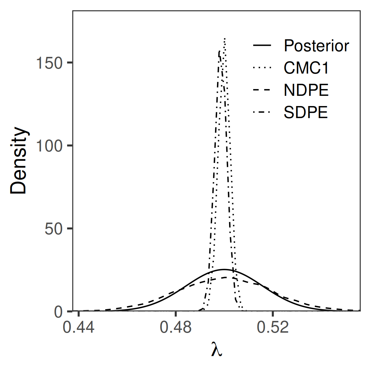
(a) KDE approximations for CMC1, NDPE and SDPE.

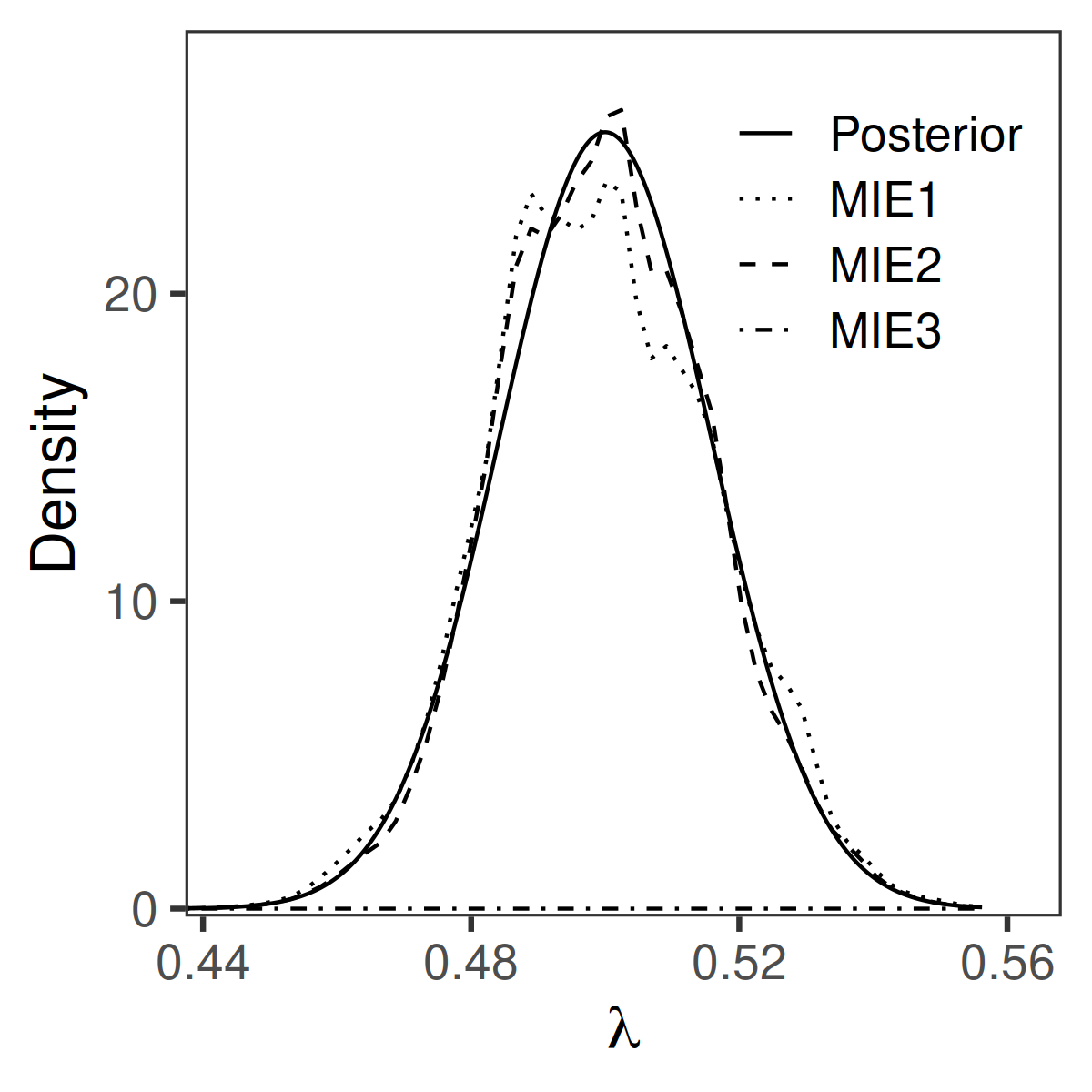
(b) KDE approximations for the MIE algorithms.

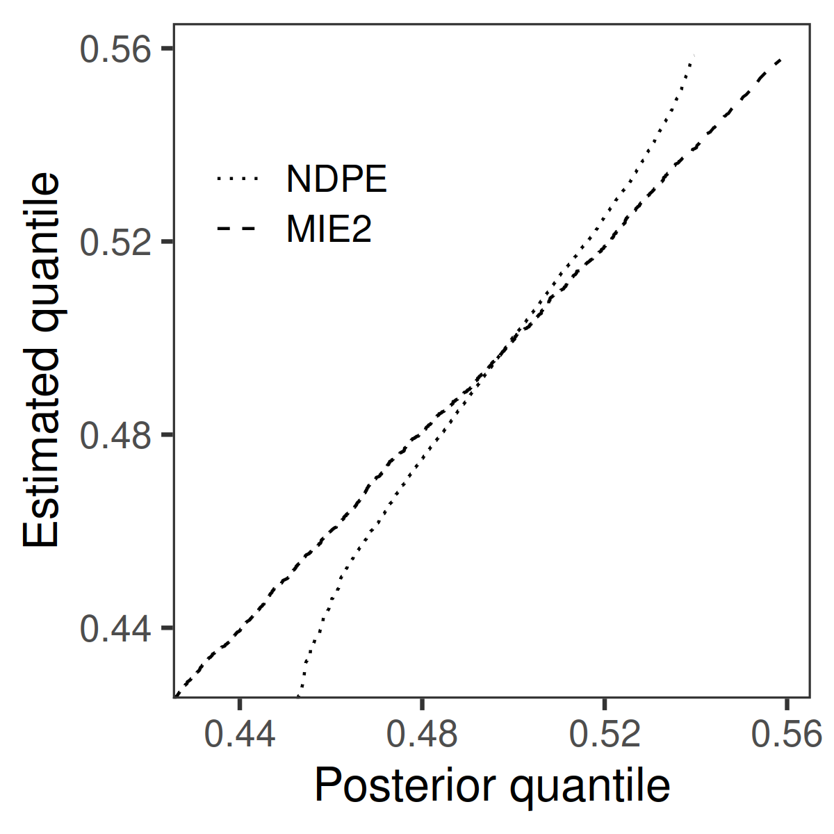
(c) Posterior quantile-quantile plot for the best of the estimators in (a) and (b).

Figure 4: Similar to figure 3 but for the example with 50% of the observations being positive. KDE bin widths are 0.002243. Results for Naive are not shown as its estimated density function appears flat on this scale.

The results of density estimation in this example are presented in Figure 4. Both CMC and DPE struggle in this example, with CMC1 in particular underestimating the tails, whilst MIE1 and MIE2 do well. NDPE is the best of the non-MIE algorithms but is poor at representing the tails of the posterior, as can be seen in Figure 4c. The results of CMC1 and SDPE are symptomatic of using an incorrect prior that is too informative.

MIE3 is poor in both of these examples, doing little better than naive pooling. This may be because the large $M$ means there are many KL divergences to estimate and almost all of them are identical (99 of them in the first example and two sets of 50 in the second). It is notable that the MIE estimators perform well even when the data are not partitioned randomly, i.e. the data parts are heterogeneous.

3.2 Multivariate normal models

In this section, $x_{i}$ for $i=1,2,\ldots,n$ follows an MVN of dimension $d$ with parameters $\mu$, the mean vector, and $\Sigma$, the covariance matrix. We study the performance of the estimators of Section 2 in posterior inference for $\mu$ with $\Sigma$ known, and for both $\mu$ and $\Sigma$, over a range of $d,n$ and $M$. In each example we simulated each $x_{i}$ from $\textrm{$\mathrm{{N}}$}_{d}\left(\mu,\Sigma\right)$, then randomly partitioned $x_{1:n}$ into $M$ parts of equal size (or as close as possible if $n$ is not divisible by $M$).

We restricted these studies to uncorrelated data, i.e. $\Sigma$ is a diagonal matrix, in order to focus on the effects of $d,n$ and $M$. The values on the diagonal, $\sigma_{1:d}^{2}$, and $\mu$ were simulated, for each condition, from

$$\sigma_{k}^{2} \sim \mathrm{{Gamma}}\left(10,1\right),k=1,2,\ldots,d,$$

$$\mu\mid\sigma_{1:d}^{2} \sim \textrm{$\mathrm{{N}}$}_{d}\left(0_{d},\frac{1}{2}\left(\sigma_{1:d}^{2}\right)^{\intercal}I_{d}\right).$$ (75)

We estimated the posterior mean of $\mu$ and $\Sigma$ and the 2.5% and 97.5% quantiles of the marginals of the posterior for each element of $\mu$ and $\Sigma$ and calculated the error for each method using Equation 70. We also estimated the KL divergence between the posterior distribution and the KDE approximation for each method using the approach explained at the start of Section 3.

In posterior inference for $\mu$ when $\Sigma$ is known, a prior is needed for $\mu$, for which we used the MVN

$$\mu\sim\textrm{$\mathrm{{N}}$}_{d}\left(\mu_{0},\Sigma_{0}\right),$$ (76)

where $\mu_{0}\in\mathbb{{R}}^{d}$ and $\Sigma_{0}$ is a $d$ by $d$ positive definite matrix. We used the uninformative prior with $\mu_{0}=0_{d}$ and $\Sigma_{0}=\mathbf{0}_{d\times d}$, so the posterior distribution is $\textrm{$\mathrm{{N}}$}_{d}\left(\bar{x},\frac{1}{n}\Sigma\right)$ where $\bar{x}:=\frac{1}{n}\sum_{i=1}^{n}x_{i}$. For CMC and DPE, the approach to fractionation implied by Equation 58 demands an MVN in the density function of which the argument of the exponential function is

$$-\frac{1}{2M}\left(\mu-\mu_{0}\right)^{\intercal}\Sigma_{0}^{-1}\left(\mu-\mu_{0}\right),$$ (77)

so the fractionated prior can be parameterised as an MVN by replacing $\Sigma_{0}$ with $M\Sigma_{0}$. When $\Sigma_{0}=\mathbf{0}_{d\times d}$ this fractionated prior is the same as the prior.

In posterior inference for both $\mu$ and $\Sigma$ we used the normal-inverse Wishart prior for $\mu$ and $\Sigma$, i.e $\left(\mu,\Sigma\right)\sim\mathrm{{NIW}}\left(\mu_{0},\kappa,\Psi,\nu\right)$ or

$$\Sigma \sim \mathrm{{IW}}\left(\Psi,\nu\right),$$

$$\mu\mid\Sigma \sim \textrm{$\mathrm{{N}}$}_{d}\left(\mu_{0},\frac{1}{\kappa}\Sigma\right),$$ (78)

where $\Psi$ is a $d$ by $d$ positive definite matrix, $\nu>0,\kappa>0$ and $\mu_{0}\in\mathbb{{R}}^{d}$. The fractionated prior using the same approach as above has a density function proportional to

$$\left|\Sigma\right|^{\nicefrac{{-\left(\nu+d+1\right)}}{{2M}}}e^{-\frac{1}{2M}\mathrm{{tr}}\left(\Psi\Sigma^{-1}\right)}.$$ (79)

We used an uninformative prior, achieved by setting $\kappa=0,\nu=0$ and $\Psi=\mathbf{0}_{d\times d}$ (which results in an improper prior). Then we can replace $\nu$ with $\nu^{*}=\frac{\nu}{M}-\frac{M-1}{M}d-\frac{M-1}{M}$ to parameterise the fractionated prior as a normal-inverse Wishart distribution (the exponential function in Equation 79 is the same as in the prior). The posterior distribution obtained using this fractionated prior is proper so long as $n,M$ and $d$ satisfy $\left\lfloor\frac{n}{M}\right\rfloor>2d$ (see Appendix A.4), which is a constraint we respect in our simulations.

For estimation, we drew $\bar{N}=1,000$ samples from each local posterior. For the LEMIE estimators, we drew an additional 1,000 samples from each of the Laplace approximations, as explained in Section 2.3. In these examples, the naive estimator of the posterior mean of $\mu$ and the CMC1 estimator are optimal because they are equivalent to the maximum likelihood estimator of $\mu$, which in this example with an uninformative prior is equal to the posterior mean.

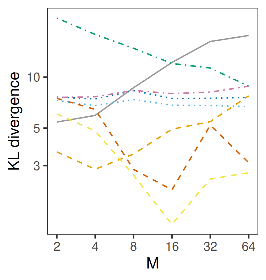
(a) KL divergence from the approximations to the posterior of $\mu$.

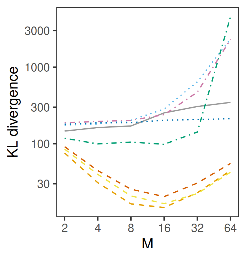
(b) KL divergence from the approximations to the posterior of $\Sigma$.

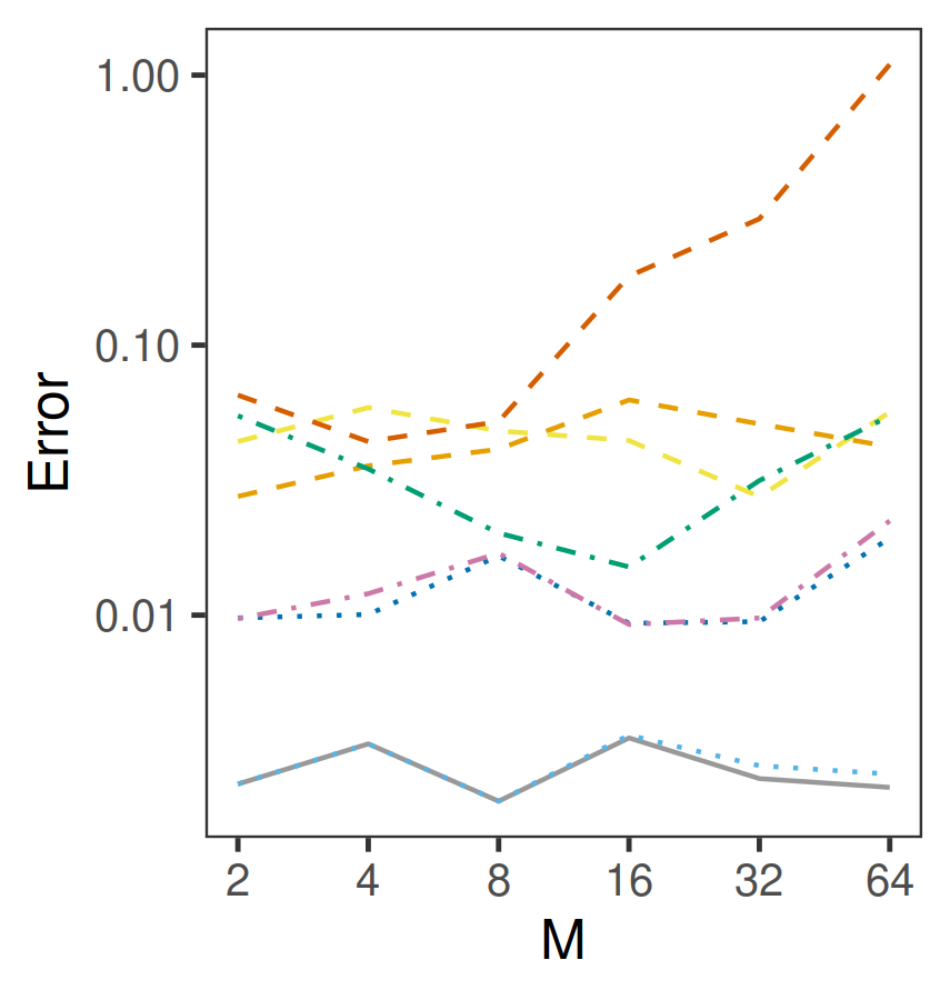
(c) Error in estimating the posterior mean of $\mu$.

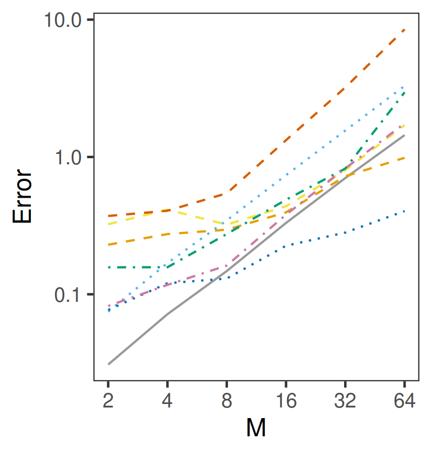
(d) Error in estimating the posterior mean of $\Sigma$.

Figure 5: Posterior estimation performance in the MVN example of Section 3.2 with $\mu$ and $\Sigma$ unknown, $d=8$ and $n=10,000$. The LEMIE methods are enhanced using Laplace samples of all 3 types.

In Figure 5 are plotted performance metrics for the simulations with $\mu$ and $\Sigma$ unknown, $d=8$ and $n=10,000$, which is one of the more challenging examples. Of the methods from Section 2.2, LEMIE using Laplace samples of all 3 types performed best; results for these are plotted against the naive, CMC and DPE methods. The approximate KL divergences for the LEMIE algorithms are generally lower than the other methods, indicating a closer approximation to the posterior. LEMIE type 1 and 2 approximate the posterior mean of $\mu$ and $\Sigma$ about as well as the other suboptimal methods. For $\Sigma$, LEMIE1 outperforms naive at $M=64$ and all other methods except CMC2. Similar results for the simulations with $d=8$ with $n=1,088$ and $n=100,000$ can be found in Appendix D.1, and the results are similar.

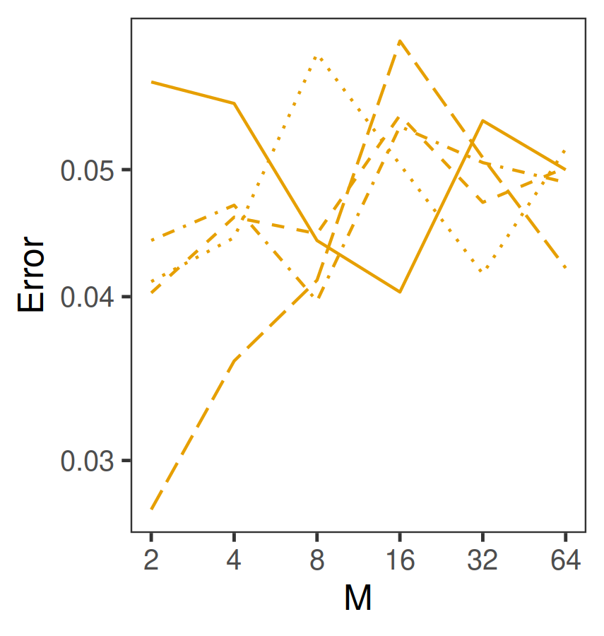
(a)

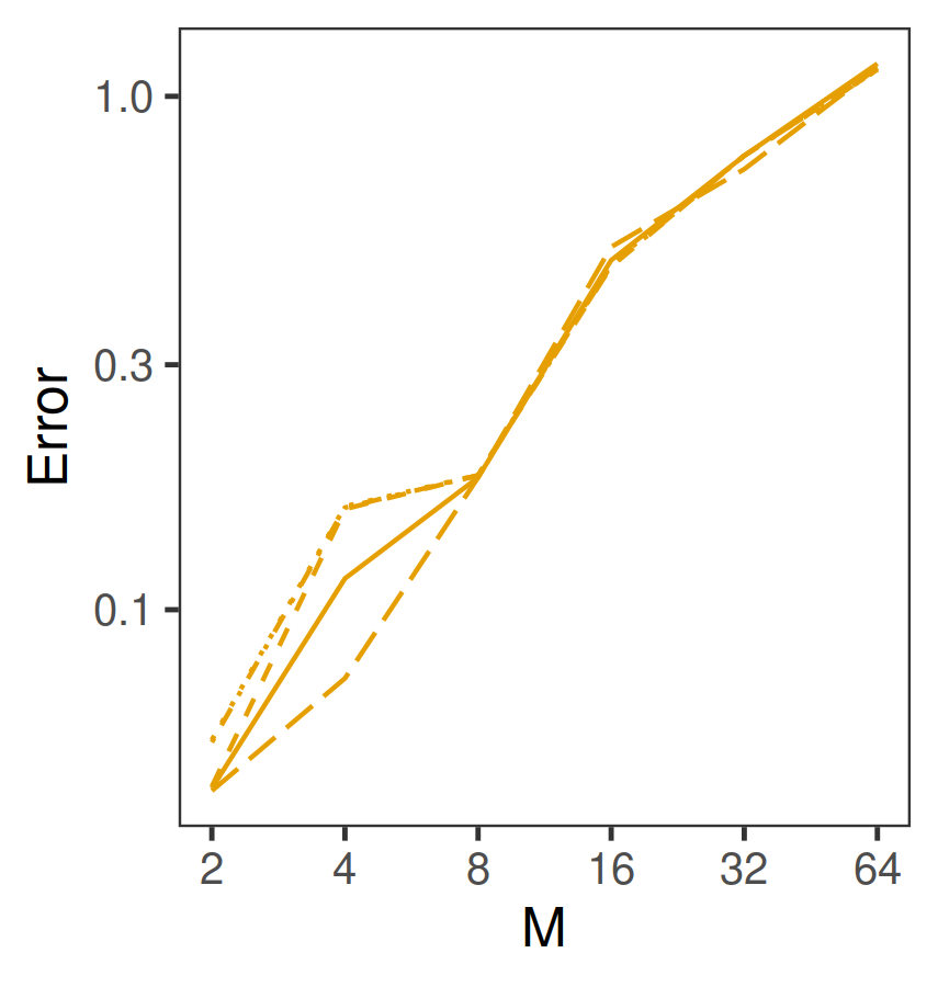
(b)

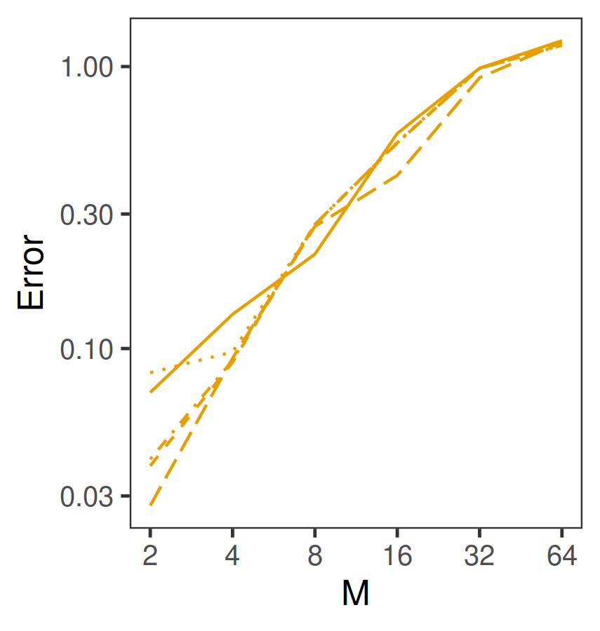
(c)

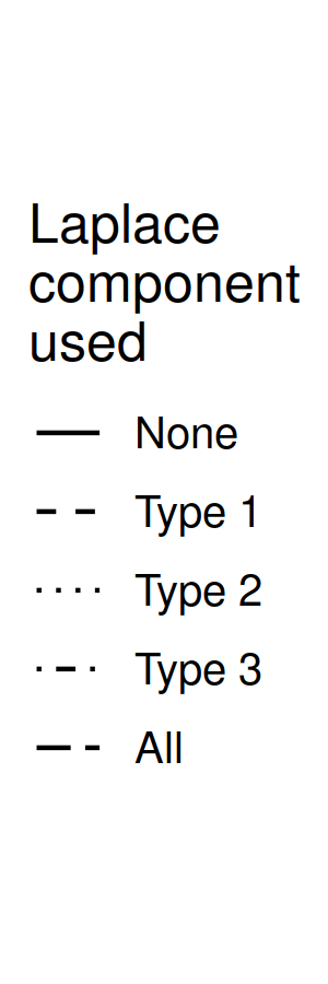
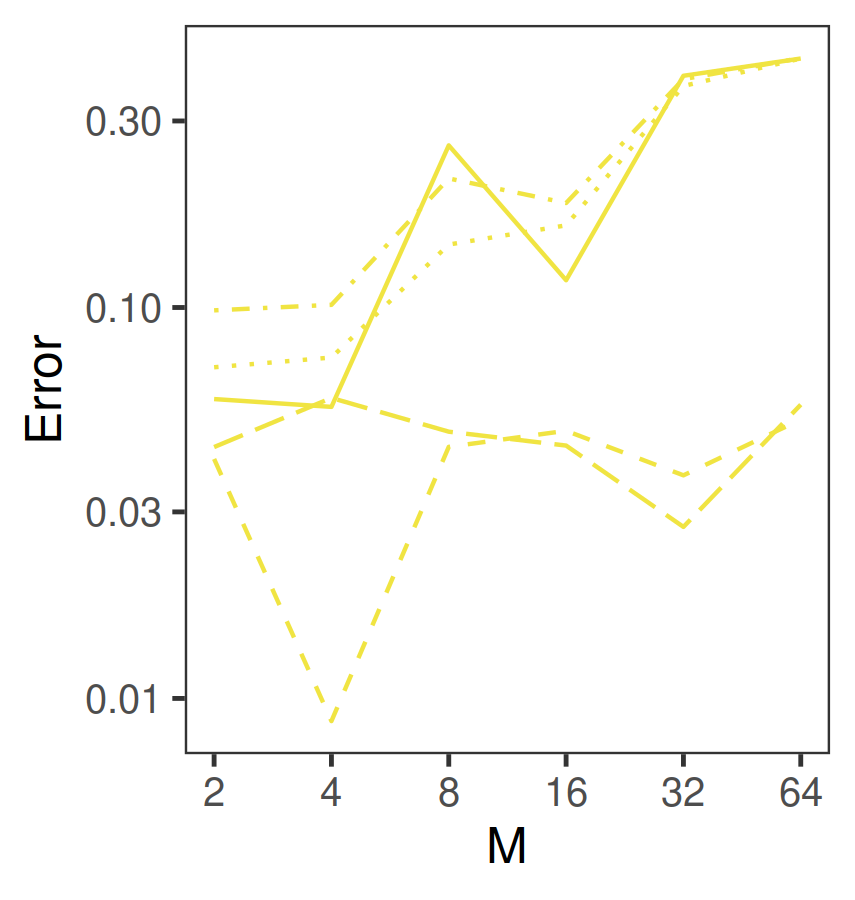
(d)

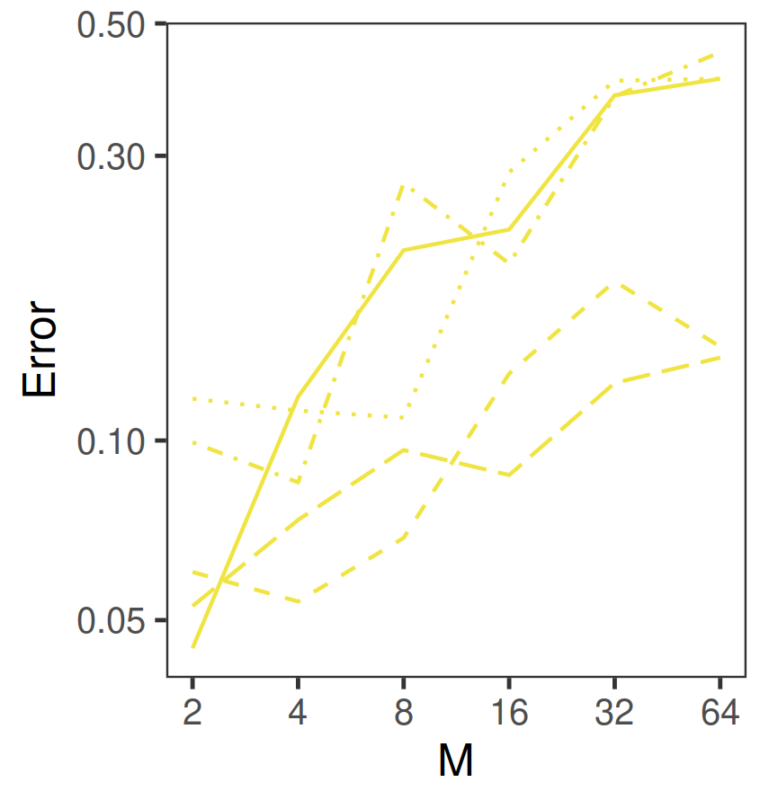
(e)

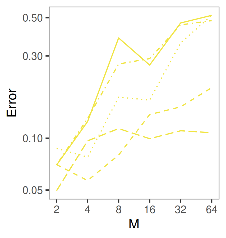
(f)

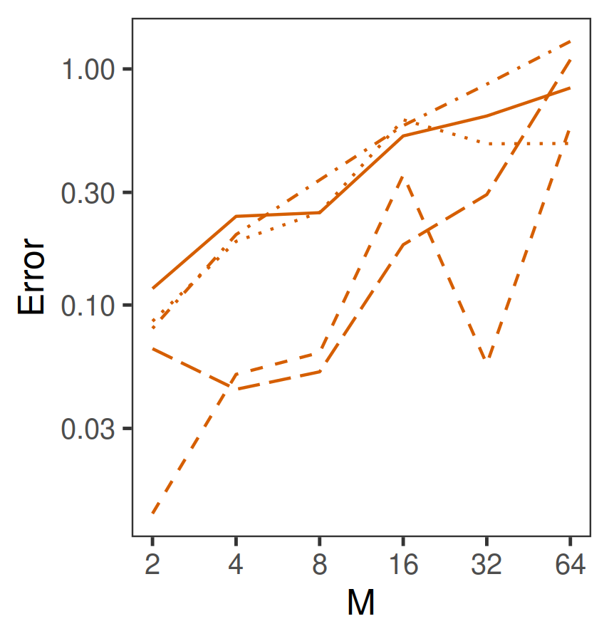
(g)

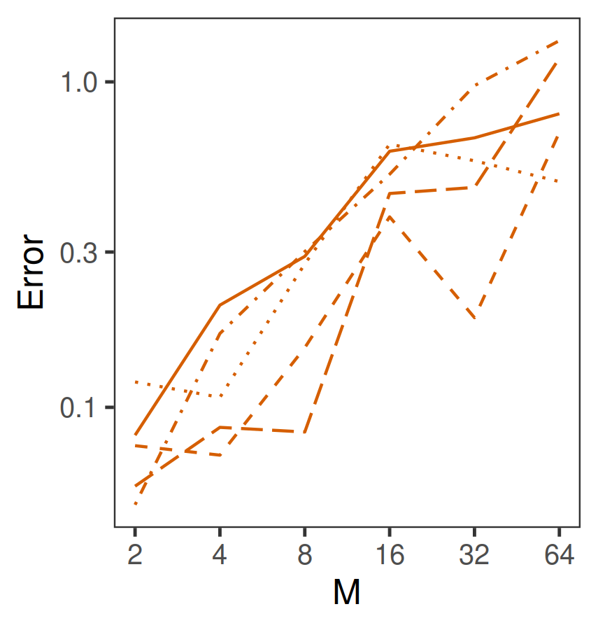
(h)

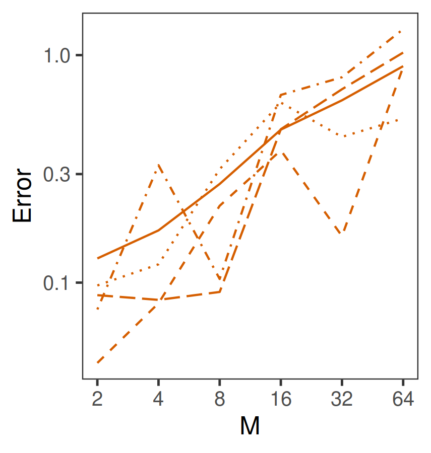
(i)

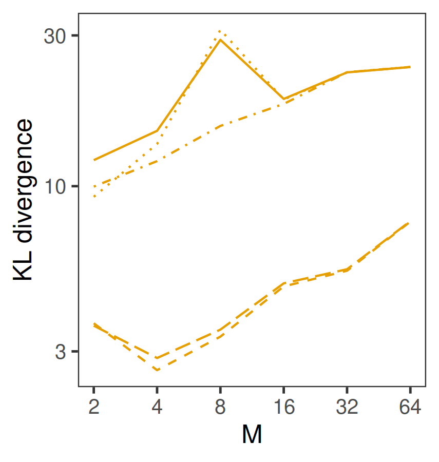
(j)

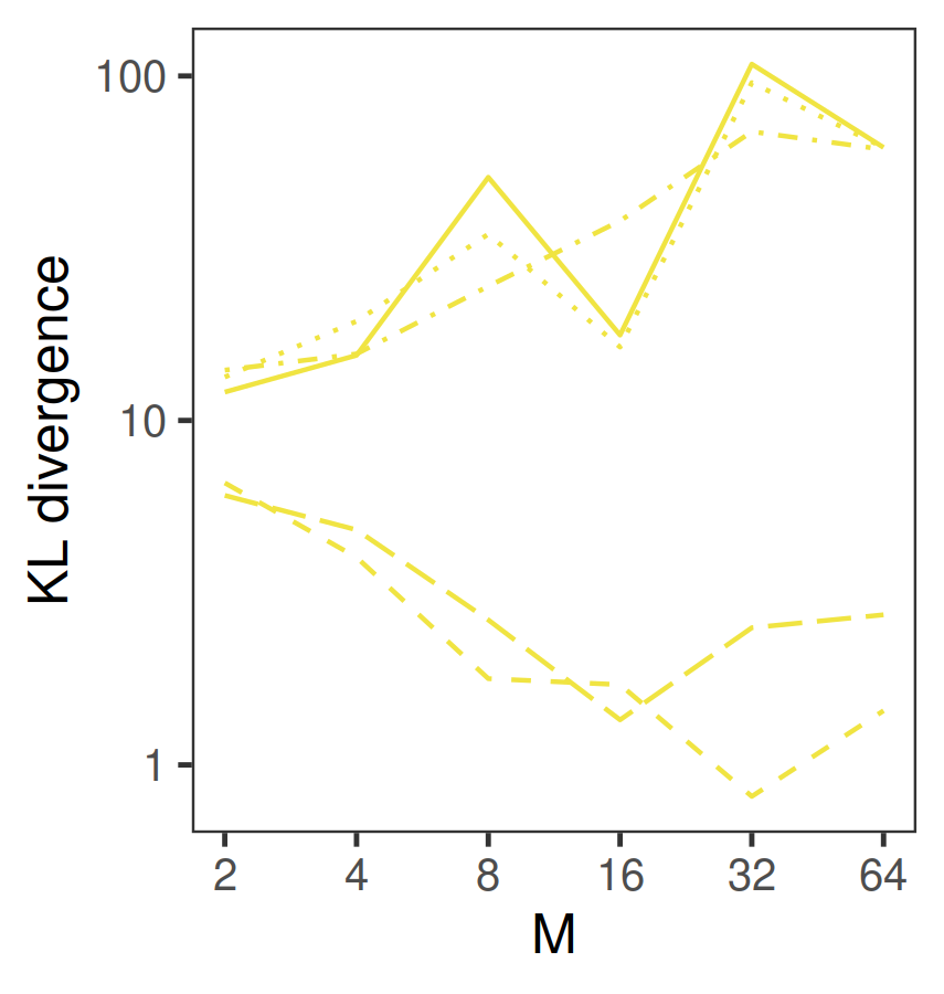
(k)

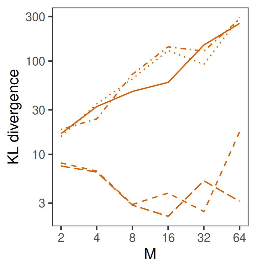
(l)

Figure 6: Posterior approximation comparisons for the algorithms from Section 2.2 approximating the $\mu$ marginal of the posterior in the MVN example with $\Sigma$ unknown and $d=8$ and $n=10,000$ of Section 3.2. The error in estimating (a)(d)(g) the posterior mean, (b)(e)(h) 2.5% quantiles of the marginals of the posterior, (c)(f)(i) 97.5% quantiles of the marginals of the posterior. (j)(k)(l) The KL divergence from the posterior to each approximation.

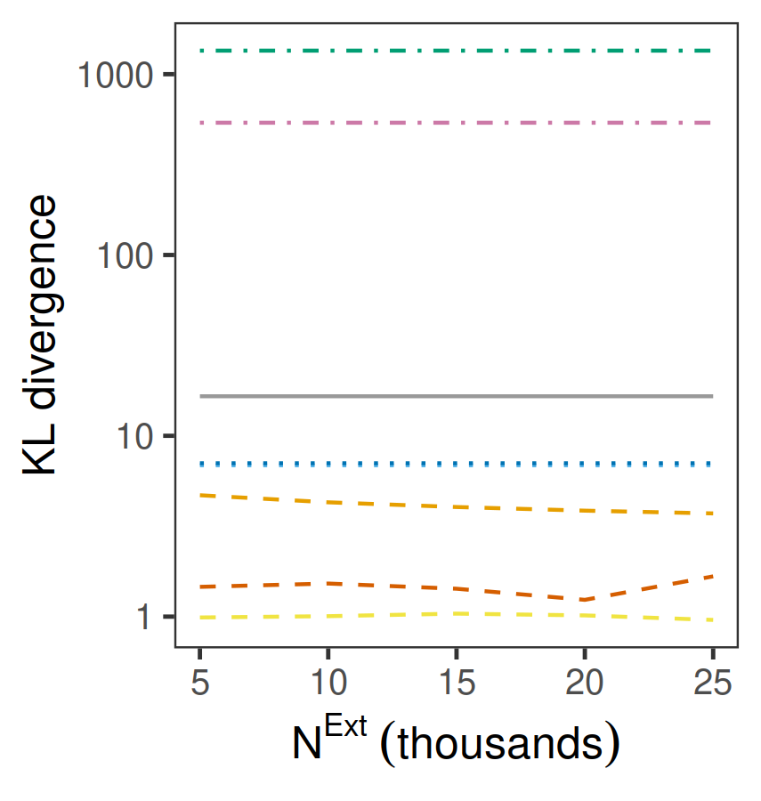
(a) KL divergence from the approximations to the posterior of $\mu$.

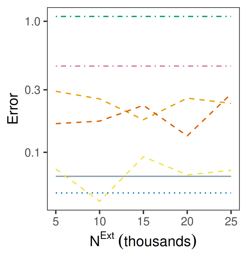
(b) Error in estimating the mean of $\mu$.

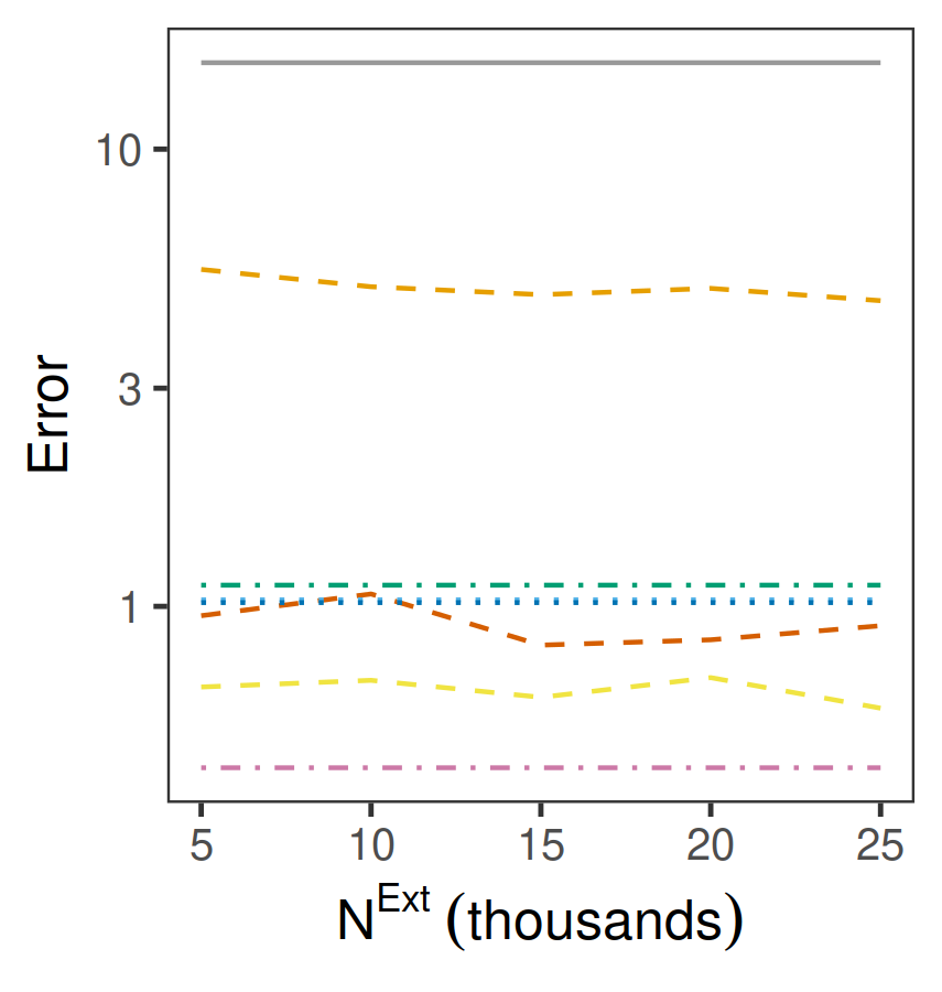
(c) Error in estimating the 2.5% quantiles of the $\mu$ marginal of the posterior.

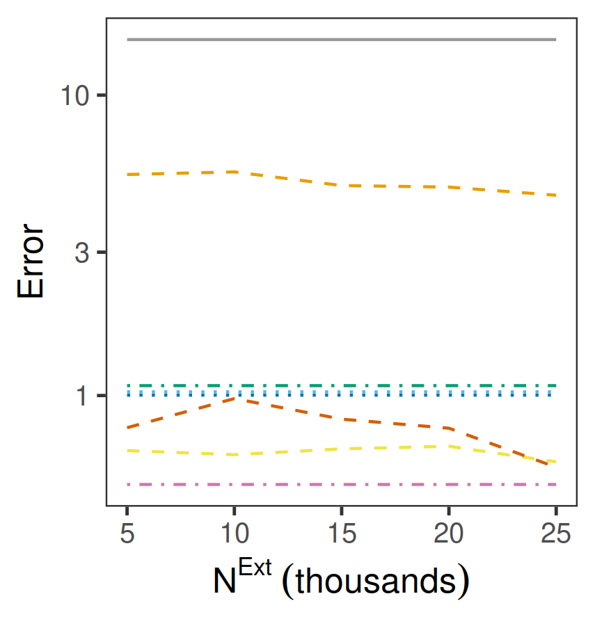
(d) Error in estimating the 97.5% quantiles of the $\mu$ marginal of the posterior.

Figure 23: Effect on performance metrics of adding more Laplace samples (of all types from Section 2.3) in the MVN example from Section 3.2 with $\Sigma$ known. $N^{\textrm{{Ext}}}$ is the total number of Laplace samples added.

Figure 6 compares across the LEMIE algorithm variants in the same example (results shown for the $\mu$ marginal of the posterior; see Appendix D.1 for a similar plot showing results for the $\Sigma$ marginal). For LEMIE1, using Laplace samples improves posterior mean estimation only for low $M$ and not clearly for estimating tail quantiles. For LEMIE2 and LEMIE3, using Laplace samples of type 1 improves estimation across all $M$; using the other Laplace types may have further benefit but this is not clear. The KL divergence is improved greatly by using Laplace samples of type 1; using samples of types 2 and 3 does not provide any further benefit. We also find that only a small number of Laplace samples are required to provide benefit and adding additional samples over a range from 5,000 to 25,000 samples does not seem to help further (Figure 23 in Appendix D.1).

			$n=1,088$			$n=10,000$
	Laplace		$d=2$	$d=4$	$d=8$	$d=2$	$d=4$	$d=8$
LEMIE1	None	$\mu$	1.221 (0.002)	5.892 (0.009)	33.43 (0.04)	1.422 (0.002)	6.95 (0.01)	23.83 (0.05)
		$\Sigma$	1.713 (0.003)	29.3 (0.03)	175.99 (0.07)	1.959 (0.002)	27.45 (0.05)	341.6 (0.2)
	Type 1	$\mu$	1.318 (0.002)	4.25 (0.01)	7.28 (0.02)	1.214 (0.002)	4.671 (0.006)	7.72 (0.02)
		$\Sigma$	1.748 (0.003)	29.28 (0.03)	175.8 (0.07)	2.05 (0.002)	10.39 (0.02)	44.6 (0.07)
	Type 2	$\mu$	1.352 (0.002)	4.604 (0.009)	33.45 (0.04)	1.256 (0.002)	6.96 (0.01)	23.84 (0.05)
		$\Sigma$	1.752 (0.003)	29.28 (0.03)	176.01 (0.07)	2.115 (0.002)	27.47 (0.05)	341.7 (0.2)
	Type 3	$\mu$	1.352 (0.002)	4.604 (0.009)	33.45 (0.04)	1.229 (0.002)	6.93 (0.01)	23.84 (0.05)
		$\Sigma$	1.753 (0.003)	29.28 (0.03)	176.01 (0.07)	2.053 (0.002)	27.44 (0.05)	265.7 (0.2)
LEMIE2	None	$\mu$	0.496 (0.005)	6.46 (0.02)	38.06 (0.07)	0.477 (0.008)	16.53 (0.03)	62 (0.09)
		$\Sigma$	0.622 (0.006)	28.25 (0.05)	537.89 (0.07)	0.986 (0.009)	23.58 (0.05)	438.1 (0.2)
	Type 1	$\mu$	0.602 (0.004)	7.39 (0.02)	190.8 (0.2)	0.275 (0.005)	1.76 (0.02)	1.44 (0.02)
		$\Sigma$	0.672 (0.006)	30.24 (0.04)	1045.1 (0.2)	0.469 (0.008)	6.93 (0.03)	44.69 (0.07)
	Type 2	$\mu$	55.29 (0.08)	299.4 (0.2)	538 (0.3)	1.49 (0.01)	17.44 (0.04)	62 (0.09)
		$\Sigma$	266.4 (0.2)	230.2 (0.1)	3478.7 (0.3)	5.36 (0.02)	36.59 (0.04)	438.5 (0.2)
	Type 3	$\mu$	3.17 (0.02)	171.4 (0.1)	155.6 (0.2)	1.41 (0.01)	9.28 (0.03)	61.2 (0.09)
		$\Sigma$	2.56 (0.01)	495.9 (0.2)	1566.2 (0.2)	2.85 (0.01)	48.8 (0.05)	261.5 (0.2)
LEMIE3	None	$\mu$	18.6 (0.04)	83.45 (0.05)	329.8 (0.2)	3 (0.01)	92.5 (0.1)	253.4 (0.2)
		$\Sigma$	24.33 (0.03)	149.37 (0.08)	928.18 (0.1)	41.89 (0.06)	213.2 (0.2)	1132.9 (0.3)
	Type 1	$\mu$	3.64 (0.02)	111.92 (0.1)	263.1 (0.2)	1.523 (0.005)	12.17 (0.01)	17.43 (0.01)
		$\Sigma$	22.43 (0.03)	206.99 (0.08)	537.6 (0.1)	1.81 (0.01)	24.11 (0.03)	64.78 (0.08)
	Type 2	$\mu$	80.58 (0.06)	48.86 (0.08)	125.9 (0.1)	14.3 (0.03)	29.9 (0.06)	294 (0.2)
		$\Sigma$	43.45 (0.07)	388.3 (0.1)	2104.9 (0.1)	14.23 (0.03)	212.1 (0.2)	1020.6 (0.2)
	Type 3	$\mu$	89.12 (0.01)	193.6 (0.2)	476.7 (0.3)	15.35 (0.01)	73.96 (0.09)	281.8 (0.2)
		$\Sigma$	97.76 (0.1)	329.5 (0.1)	1323.4 (0.2)	20.31 (0.03)	196.69 (0.1)	685.8 (0.3)
Vanilla		$\mu$	0.03 (0.01)	0.52 (0.03)	6.71 (0.08)	0.02 (0.01)	0.49 (0.02)	7.3 (0.09)
		$\Sigma$	0.16 (0.02)	13.6 (0.1)	177.9 (0.4)	0.13 (0.02)	14 (0.1)	179.9 (0.4)
Naive		$\mu$	3.9794 (2e-04)	7.7391 (9e-04)	21.35 (0.02)	3.93 (1e-04)	8.066 (0.001)	17.6 (0.02)
		$\Sigma$	5.8749 (8e-04)	25.69 (0.02)	140.15 (0.05)	5.8092 (7e-04)	31.59 (0.03)	346.9 (0.2)
CMC2		$\mu$	0.04 (0.01)	0.53 (0.03)	7.57 (0.09)	0.01 (0.01)	0.53 (0.03)	7.58 (0.09)
		$\Sigma$	1.01 (0.01)	55.7 (0.1)	255.90125 (3e-05)	0.35 (0.02)	20.7 (0.2)	212.5 (0.5)
SDPE		$\mu$	3 (0.1)	3.96 (0.1)	19 (0.2)	0.07 (0.01)	0.73 (0.03)	8.83 (0.1)
		$\Sigma$	67709 (129)	222621 (132)	3839.1 (0.8)	256 (2)	249 (1)	2306 (5)

Table 1: The KL divergence from the $\mu$ and $\Sigma$ marginals of the posterior to each approximation in the example of Section 3.2 with $\Sigma$ unknown and $M=64$. Standard errors for each estimate are shown in parentheses.

Table 1 presents approximate KL divergences from the $\mu$ and $\Sigma$ marginals of the posterior to the approximations, with $M=64$. This includes the Monte Carlo estimator using $N^{*}=1,000$ samples drawn directly from the posterior, which we label “Vanilla”, and the best performing of each of the CMC and DPE estimators. In approximating the $\mu$ marginal of the posterior, the normality assumptions of CMC are met so it is unsurprising that CMC2 does almost as well as Vanilla. We found that it is actually possible to do better than Vanilla with LEMIE in the most difficult examples (larger dimension $d$). This is likely because LEMIE uses all $\bar{N}M$ samples, which in this case is 64,000, in estimators. We also find that LEMIE can do better than CMC or DPE in approximating the $\Sigma$ marginal of the posterior than the other methods, which we suggest is because the CMC and DPE methods struggle with deviations from normality such as in the inverse-Wishart distribution.

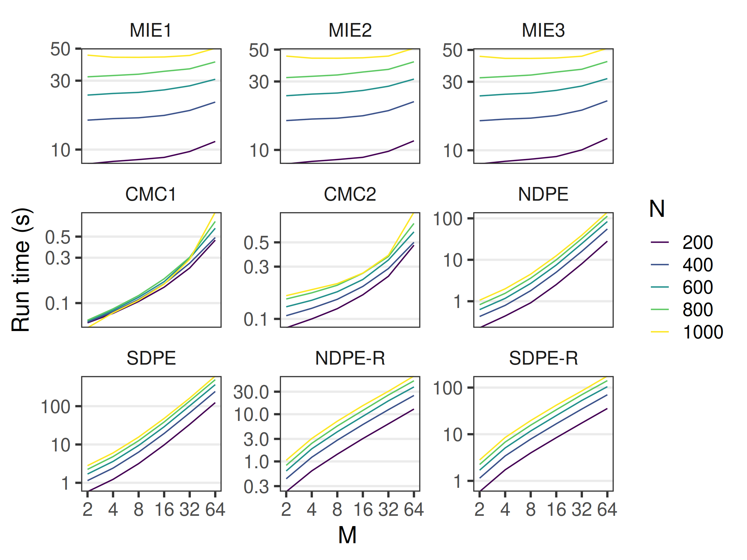
Figure 7: Run times for each algorithm from Section 2 (excluding Laplace samples) in the MVN example with $\mu$ and $\Sigma$ unknown, $d=8$ and $n=10,000$. $N$ is the number samples drawn from each local posterior ($\bar{N}$ in the text). NDPE-R and SPDE-R are the recursive versions of the algorithms explained in Section 2.5.2 using pairwise pooling of the local posteriors.

Figure 7 presents the time taken, in seconds, to run each algorithm across simulations with $d=8$ and $n=10,000$ for a range of $M$ and for different sample sizes $\bar{N}$. These run times are exclusive of the time taken to draw samples from the local posteriors, and multiple CPU core parallelisation was used as much as possible (using the parallel R package from R Core Team, (2020) and running on a 64 core AWS EC2 instance). The MIE algorithms’ timings are for the methods of Section 2.2 without any Laplace samples. The run times of all methods appear to increase exponentially with $M$. The MIE algorithms have a relatively gentle exponential increase because the majority of the computation is in likelihood evaluations which can be performed in parallel when there are $M$ cores available. The MIE algorithms seem to have more overhead, unrelated to $M$, but for large $M$ they are faster than the DPE algorithms except for the recursive version of NDPE. CMC is very fast over this range of $M$; its hardest computations are calculating the sample covariance matrices, which can be done in parallel.

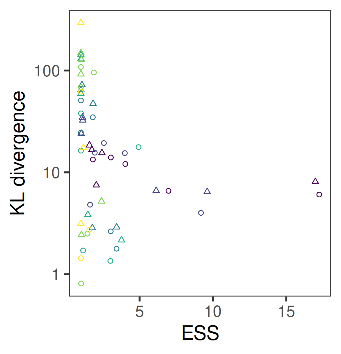
(a) KL divergence vs ESS.

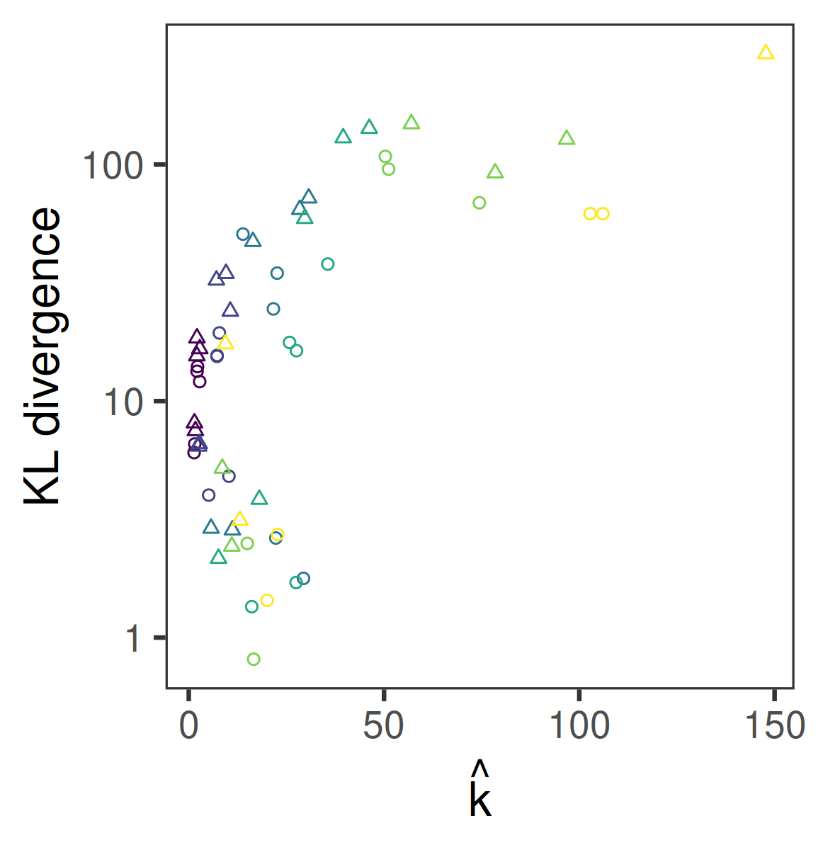
(b) KL divergence vs $\hat{{k}}$.

Figure 8: For the simulated examples of Section 3.2 with $d=8$ and $n=10,000$, KL divergences Equation 73 from the LEMIE approximations (of all types defined in Section 2.3.1) to the posterior of $\mu$ using the approach explained in Section 3 against the performance metrics of Section 2.4.

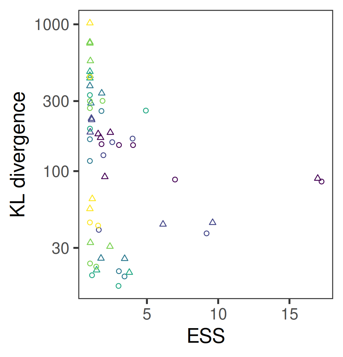
(a) KL divergence vs ESS.

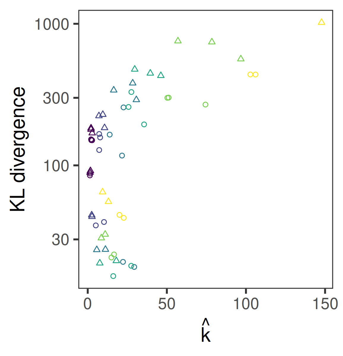
(b) KL divergence vs $\hat{{k}}$.

Figure 9: Similar to Figure 8 but of the KL divergences from the LEMIE approximations to the $\Sigma$ marginal of the posterior.

Figures 8 and 9 plot approximate KL divergences on a log scale against the estimator diagnostics ESS and $\hat{{k}}$ for LEMIE 1 and 2 using Laplace types 1, 2, 3, all 3 and none in the $d=8$ and $n=10,000$ examples. By eye, it looks like these diagnostics may be predictive of performance, at least relatively, comparing one estimator against another. We did not include LEMIE1 in Figures 8 and 9 for clarity, because ESS does not appear to be a useful predictor of performance for LEMIE1 (although $\hat{{k}}$ does). Figures including LEMIE1 can be found in Appendix D.1.

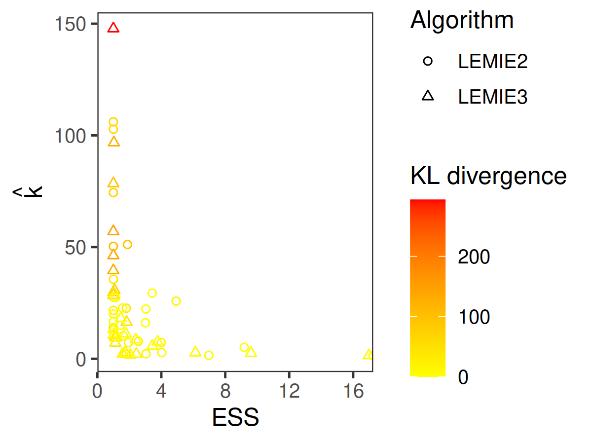
(a) Approximating the $\mu$ marginal of the posterior.

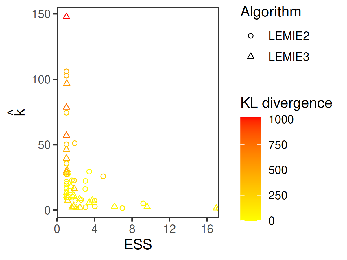
(b) Approximating the $\Sigma$ marginal of the posterior.

Figure 10: For the simulated examples of Section 3.2 with $d=8$ and $n=10,000$, KL divergences from the LEMIE approximations to the $\mu$ and $\Sigma$ marginals of the posterior using the approach explained in Section 3 against the performance metrics of Section 2.4.

As an attempt to quantify the value of ESS and $\hat{{k}}$ as predictors of performance, we looked to fit a gamma GLM to these data. Fitted GLM results using all LEMIE 1, 2 and 3 results, and for LEMIE 2 and 3 only, can be found in Appendix D.1.1. The residual deviances suggest there is predictive value in the performance metrics. For the $\mu$ marginal of the posterior, the log mean of KL divergence increases 0.032 per unit increase in $\hat{{k}}$ (standard error 0.003) and decreases -0.057 per unit increase in ESS (s.e. 0.038, model excludes LEMIE1). For the $\Sigma$ marginal of the posterior, the log mean of KL divergence increases 0.021 with a unit increase in $\hat{{k}}$ (s.e. 0.003) and decreases -0.030 with a unit increase in ESS (s.e. 0.032, model excludes LEMIE1). The existence of a positive relationship for $\hat{{k}}$ is clear whilst the negative relationship of ESS, which is clearer without LEMIE1 than with it, is not statistically significant under this model. The interaction of ESS and $\hat{{k}}$ does not appear to be usefully related to KL divergence (see estimates in Appendix D.1.1). These results provide some validation for the judgement by eye that ESS and $\hat{{k}}$ are useful, but the gamma GLM model may not be the best way to do this. In particular there is heteroscedasticity visible in Figures 8 and 9, although this might be explained between ESS and $\hat{{k}}$ when both are used as predictors of KL divergence. This joint relationship is depicted in Figure 10.

3.3 Logistic regression

We look at two logistic regression simulations, replicating those from Scott et al., (2016) and Neiswanger et al., (2013). The model is

$$y_{i}\sim\mathrm{{Binom}}\left(c_{i},\mathrm{{logit}}^{-1}\left(x_{i}^{\intercal}\theta\right)\right),i=1,2,\ldots,n,$$ (80)

where $\mathrm{{logit}}^{-1}$ is the inverse logit function, $x_{i}\in\mathbb{{R}}^{p},c_{i}\in\mathbb{{N}},y_{i}\in\mathbb{{N}}$ with $y_{i}\leq c_{i}$ and $\theta\in\mathbb{{R}}^{p}$, which is the posterior estimand of interest given data $\left\{x_{i},c_{i},y_{i};i=1,2,\ldots,n\right\}$.

For sampling from the local posteriors in these examples, we employ the Gibbs sampler of Polson et al., (2013). A brief explanation of this is provided in Appendix C. We will compare the methods’ estimates of the posterior mean, 2.5% and 97.5% quantiles of the marginals of the posterior using error function Equation 70. Since the posterior is not available in analytic form, we must estimate the true values. We do this using the same MCMC algorithm with the unpartitioned data, running the sampler for longer than the local posterior samplers for greater precision in the ground truth: 2,000,000 samples with the first 50% discarded as burn-in.

3.3.1 Simulation of Scott et al., (2016)

We use the same data as Scott et al., (2016), which is reproduced in their Table 1 (a) and consists of 10,000 binary outcomes with $p=5$ binary predictor variables. The $c_{i}$ outcomes with the same combination of predictor variables $x_{i}$ can be grouped as integer $y_{i}$ to use the model form of Equation 80.

It is not clear what prior distribution or MCMC algorithm is used by Scott et al., (2016), so we took our own initiative and used a $\mathrm{{N}}_{p}\left(0_{p},2.5^{2}I_{p}\right)$ prior and sample $\bar{N}=400,000$ times from each local posterior, discarding the first 50% as burn-in. The fractionated prior used for CMC and DPE is $\mathrm{{N}}_{p}\left(0_{p},2.5^{2}MI_{p}\right)$ (see Equation 77). Whilst Scott et al., (2016) use $M=100$, we looked at performance over a range of $M$ to study the effect of this on performance, as in the simulations in Section 3.2. For each $M$ we partitioned the data uniformly at random into $M$ parts and ran the Gibbs sampler using each data part independently.

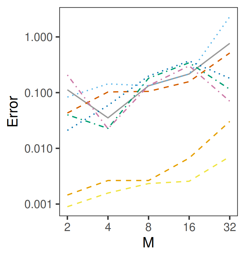
(a) Error in estimating the posterior mean of $\theta$.

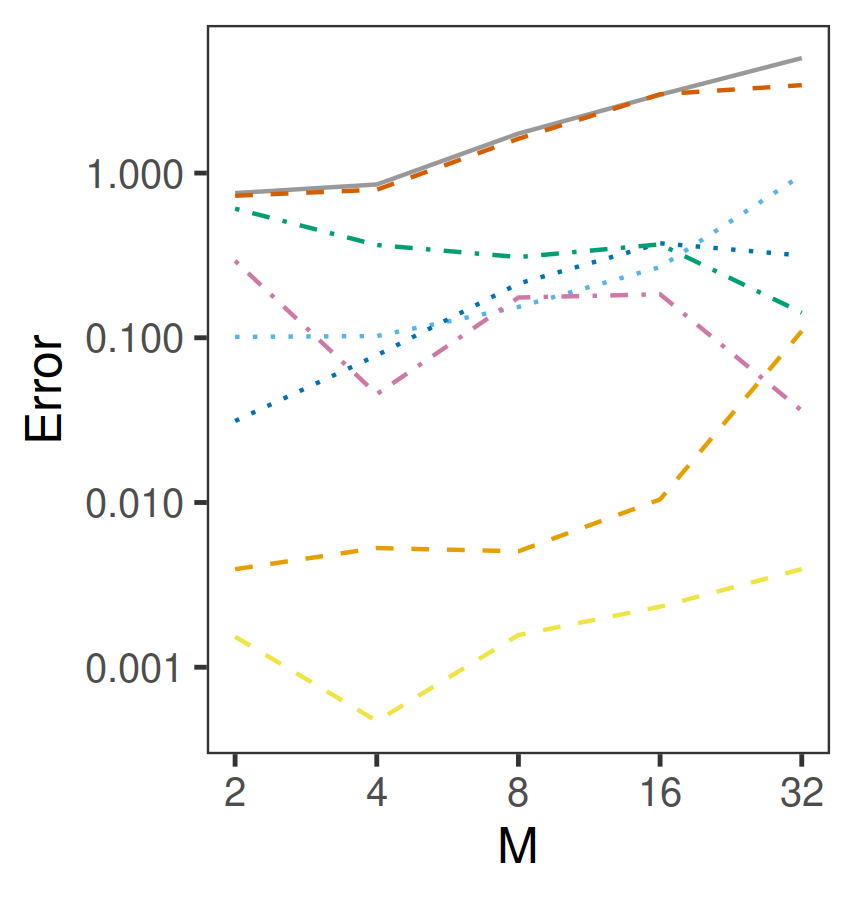
(b) Error in estimating the 2.5% quantiles of the marginals of the posterior.

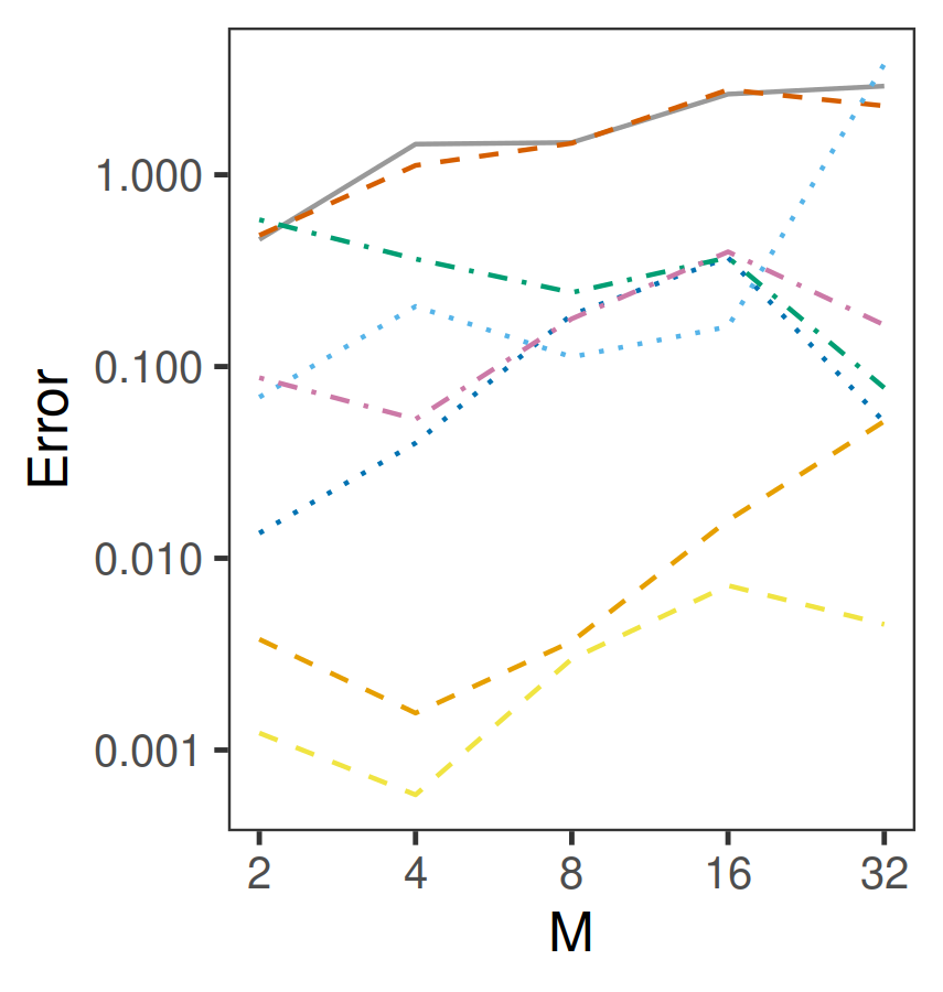
(c) Error in estimating the 97.5% quantiles of the marginals of the posterior.

Figure 11: Posterior approximation comparisons for $\theta$ in the logistic regression example of Section 3.3.1 due to Scott et al., (2016).

In Figure 11 are plotted the errors in estimating the posterior mean of $\theta$ and in estimating the 2.5% and 97.5% quantiles of the marginals of the posterior. Using Laplace samples of any type was not found to provide any benefit to the estimators of Section 2.2, so results are plotted for methods without Laplace enrichment. MIE 1 and 2 were found to be more accurate at estimating the posterior mean and quantiles than any other method across all $M$.

(a)

(b)

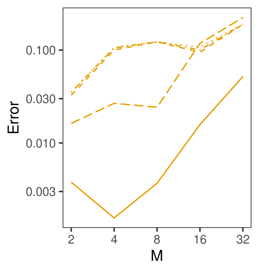
(c)

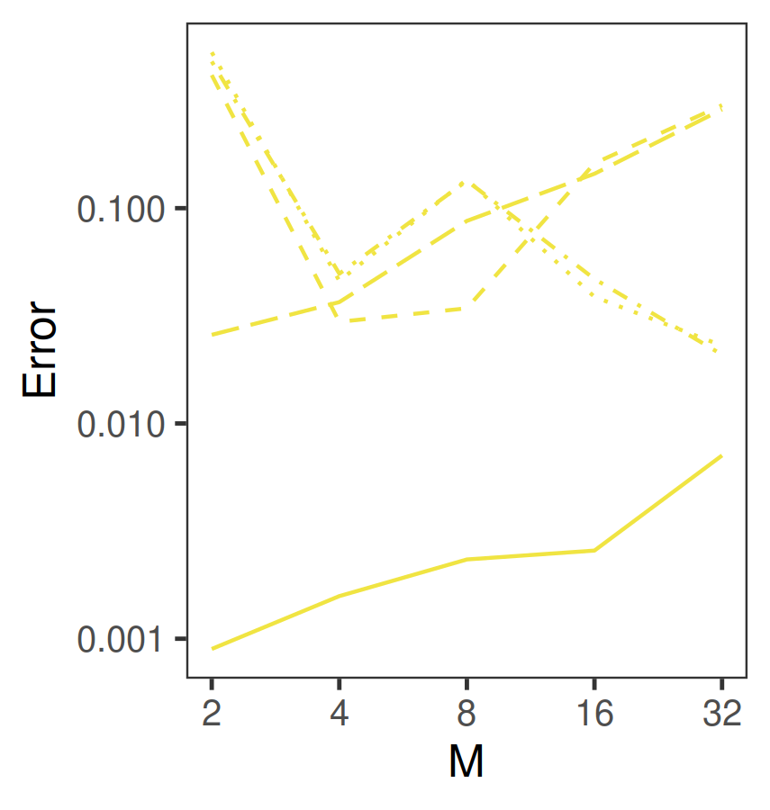
(d)

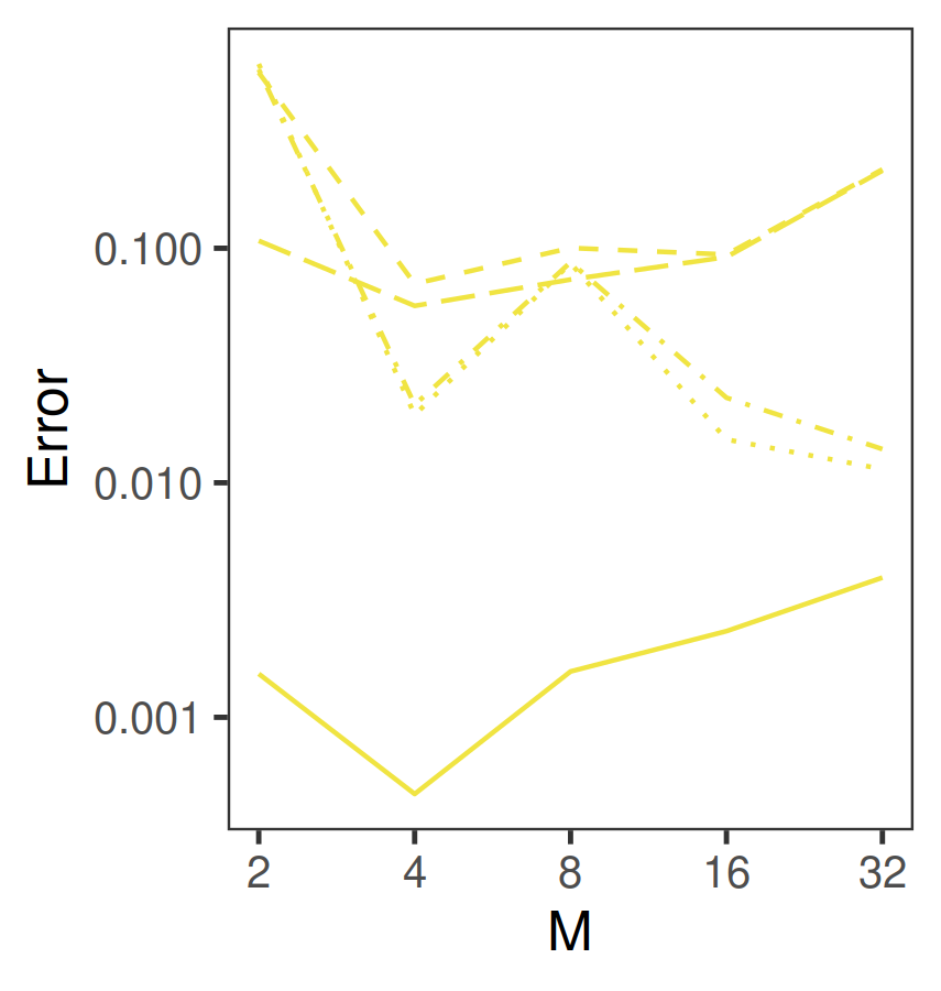
(e)

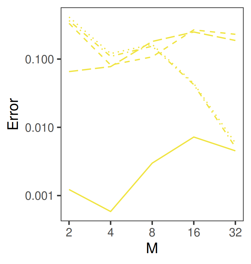
(f)

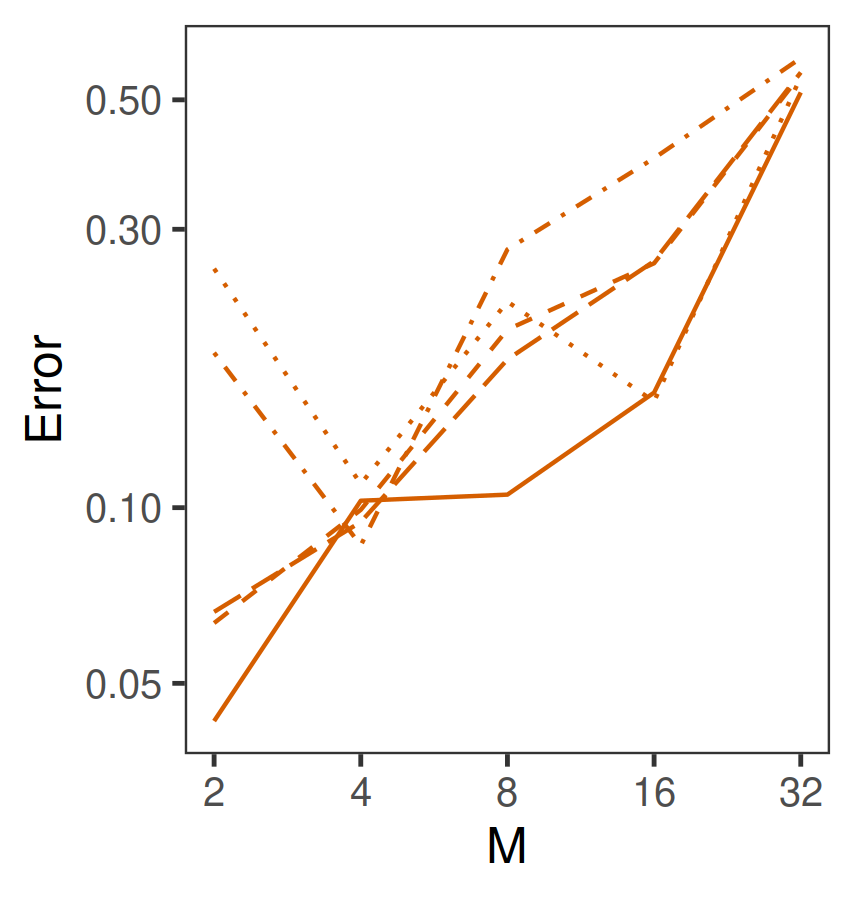
(g)

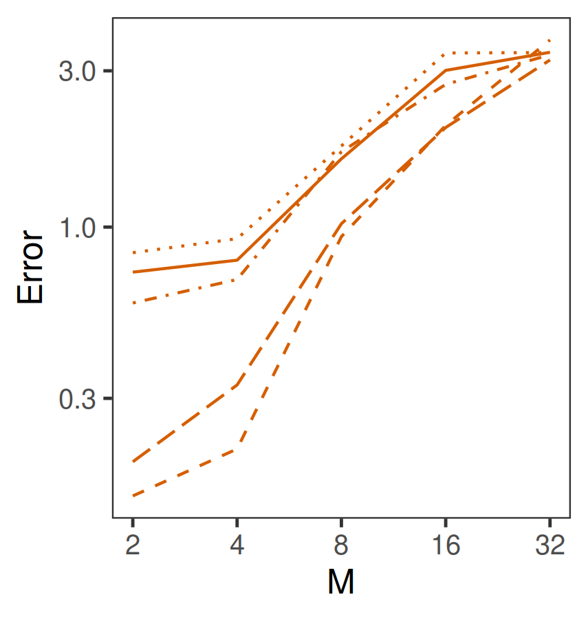
(h)

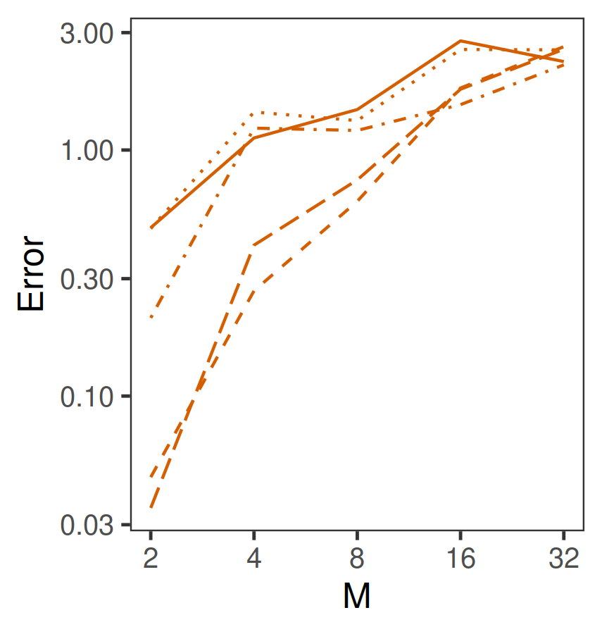
(i)

Figure 12: Posterior approximation comparisons for the algorithms from Section 2.2 in the logistic regression example of Section 3.3.1 due to Scott et al., (2016). The error in estimating (a)(d)(g) the posterior mean, (b)(e)(h) the 2.5% quantiles of the marginals of the posterior, (c)(f)(i) the 97.5% quantiles of the marginals of the posterior.

Figure 12 compares the methods of Section 2.2 in estimating the posterior mean and tail quantiles with the addition of Laplace samples. For LEMIE 1 and 2, the trend suggests using Laplace samples may become more beneficial at large $M$, but up to $M=32$ the estimator with no Laplace samples is better. LEMIE3 does not perform any better than the other methods in this example, but does appear to benefit from using Laplace samples in estimating the tail quantiles, particularly Laplace samples of type 1. We found that adding Laplace samples numbering from $1\times 10^{6}$ to $2.5\times 10^{6}$ samples does not seem to improve performance (Figure 24 in Appendix D.2).

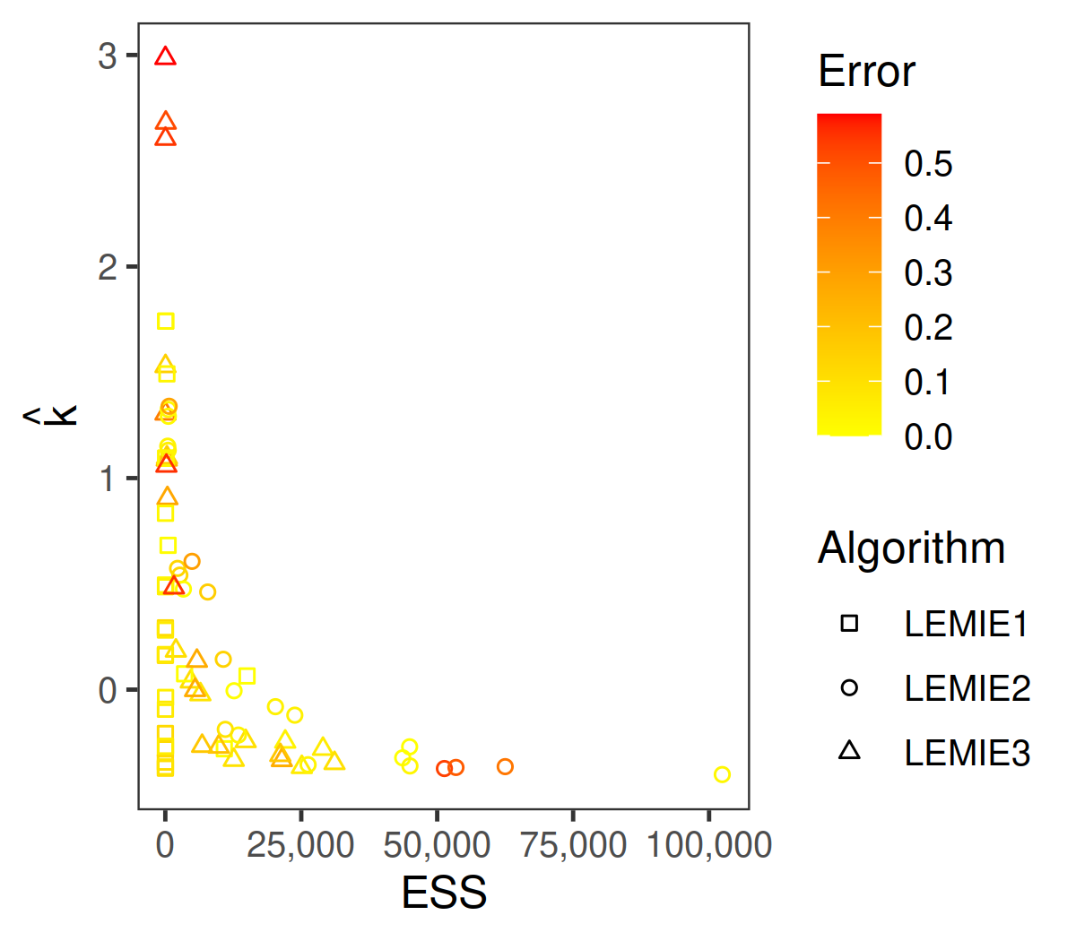
(a) Example of Section 3.3.1.

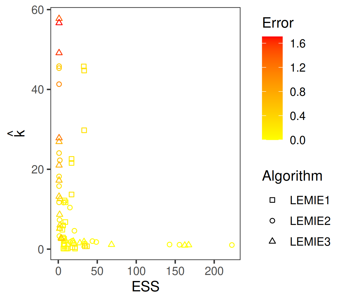
(b) Example of Section 3.3.2.

Figure 13: For the logistic regression examples in Section 3.3, error in estimating the mean of $\theta$ for the LEMIE approximations (of all types defined in Section 2.3.1) and for all $M$ considered against the performance metrics of Section 2.4.

Figure 13a plots the error in estimating $\theta$ for all LEMIE results (all types of Laplace samples and none) and in all $M$ simulations against the ESS and $\hat{{k}}$ diagnostics. As in the examples of Section 3.2, ESS and $\hat{{k}}$ are broadly related to performance. However, there are some results with low ESS and high $\hat{{k}}$ which perform relatively well, and some with high ESS and low $\hat{{k}}$ which perform relatively poorly. Those latter results were for the LEMIE2 estimator and $M=2$. The result plotted in the bottom right corner, having the greatest ESS, low $\hat{{k}}$ and low error, was also for LEMIE2 and $M=2$ but using no Laplace samples.

With this many samples per local posterior, we run into memory issues using the LEMIE algorithm when $M$ is large. This is why we only looked up to $M=32$. This is not an insurmountable barrier to using LEMIE with large $M$: if the likelihood calculations are implemented with careful memory management the space requirements can be converted to additional time requirements (although the time requirement can be substantial when $\bar{N}M$ is large). If the purpose of parallelising Bayesian computation is to speed it up, this may present a limit to the usefulness of the algorithm. We did not look at cross entropy in this example because the KDE calculations with $\bar{N}M$ samples is prohibitively slow for large $M$.

3.3.2 Simulation following Neiswanger et al., (2013)

The simulated logistic regression of Neiswanger et al., (2013) uses predictors $x_{i}\in\mathbb{{R}}^{p}$ with $p=50$ and $n=50,000$ data realisations ($c_{i}=1$ for all $i$ in the model framework used at the start of Section 3.3). The parameters $\theta$ and each realisation $x_{i}$ were simulated from $\mathrm{{N}}_{p}\left(0_{p},I_{p}\right)$. As in the example in Section 3.3.1 we partitioned the data uniformly at random into $M$ parts. Neiswanger et al., (2013) use the No U-turn Hamiltonian Monte Carlo sampler implemented in Stan (Stan Development Team, (2022)). It is not clear what prior distribution they use; we used a $\mathrm{{N}}_{p}\left(0_{p},2.5^{2}I_{p}\right)$ prior and sampled $\bar{N}=400,000$ times from each local posterior, discarding the first 50% as burn-in, using the Gibbs sampler of Polson et al., (2013). As in Section 3.3.1, the fractionated prior used for CMC and DPE is $\mathrm{{N}}_{p}\left(0_{p},2.5^{2}MI_{p}\right)$.

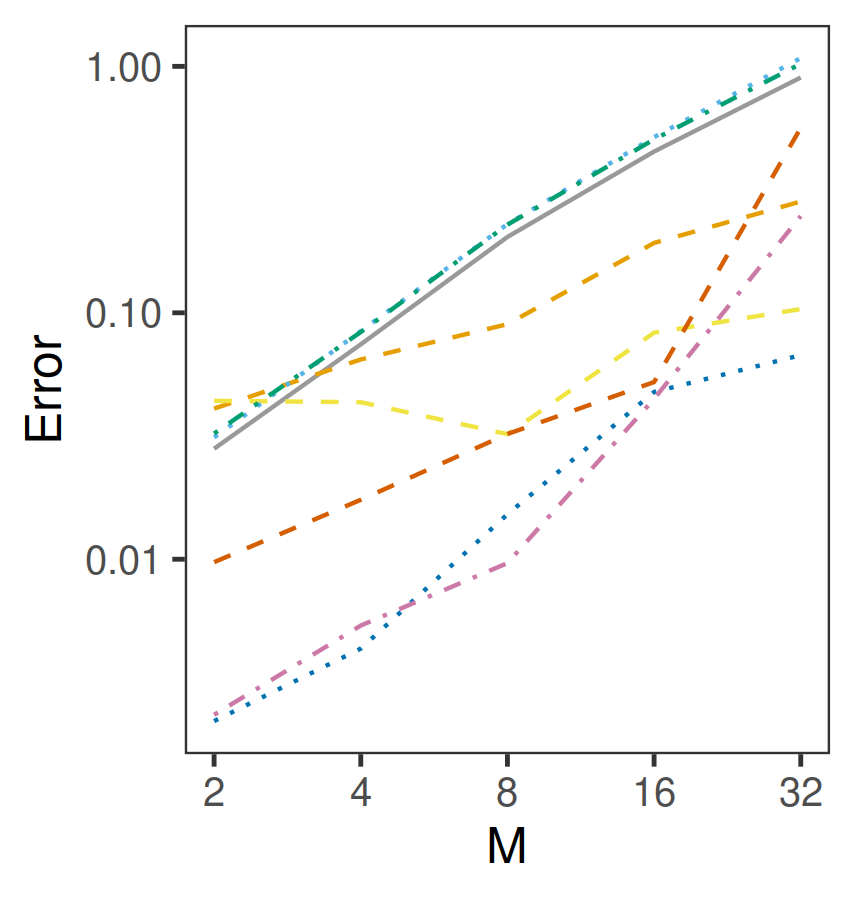
(a) Error in estimating the posterior mean of $\theta$.

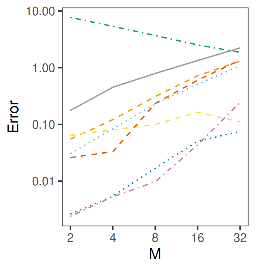
(b) Error in estimating the 2.5% quantiles of the marginals of the posterior.

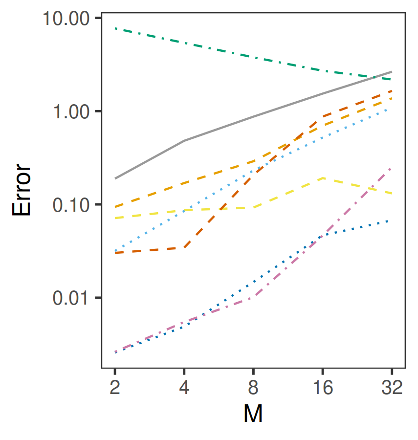
(c) Error in estimating the 97.5% quantiles of the marginals of the posterior.

Figure 14: Posterior approximation comparisons for $\theta$ in the logistic regression example of Section 3.3.2.

Performance results are presented in Figure 14. CMC2 and SDPE perform consistently well across the range of $M$ considered. The LEMIE algorithms are also fairly reliable across $M$, and for $M>8$ the best performing LEMIE algorithm does almost as well as the best of CMC or DPE at estimating the posterior mean and tail quantiles. CMC and DPE are better suited to this example than that in Section 3.3.1 because of the large $n$, meaning the posterior is better approximated by an MVN. It is notable that LEMIE does almost as well as any other method when $M$ is large given the relatively large dimension $p$.

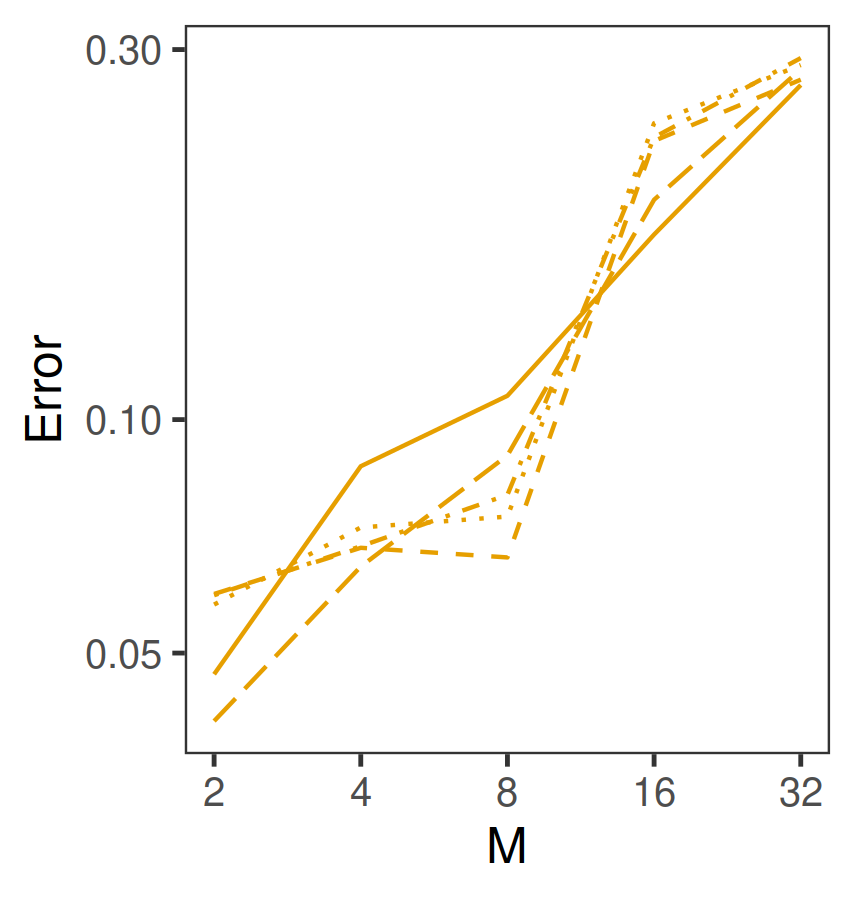
(a)

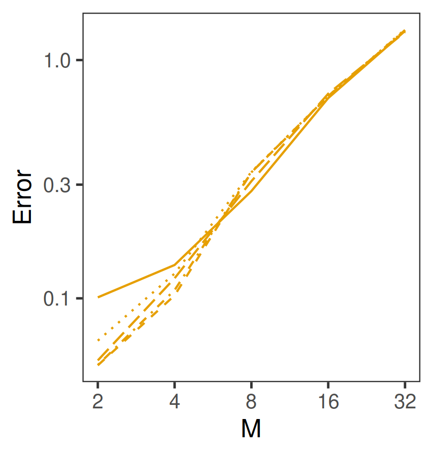
(b)

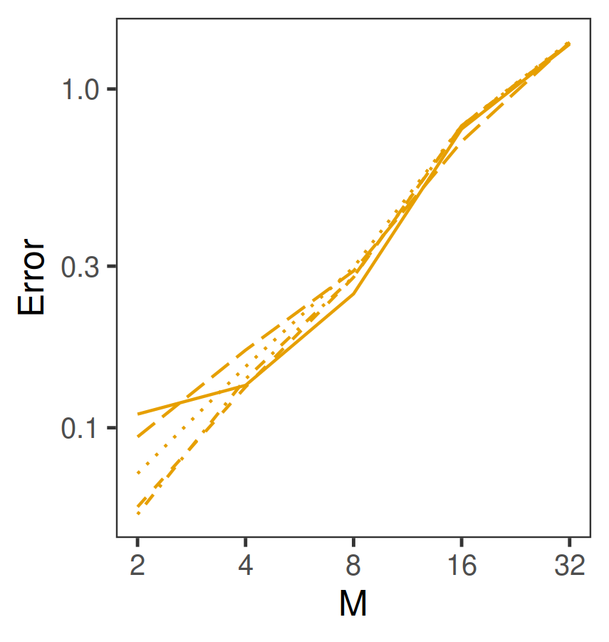
(c)

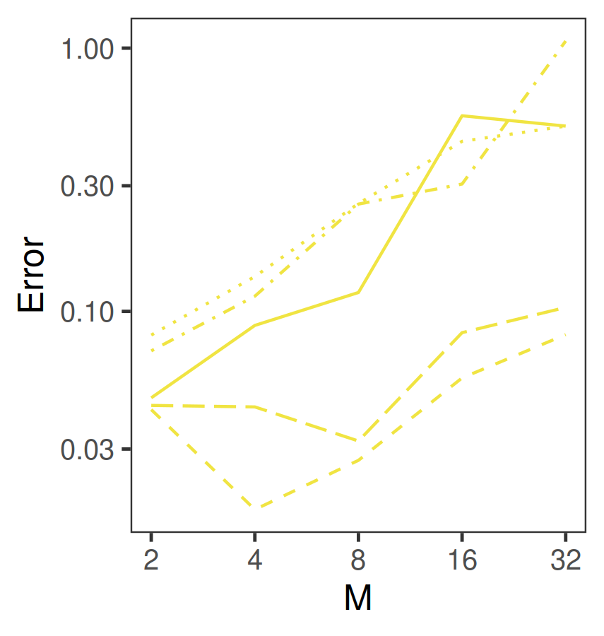
(d)

(e)

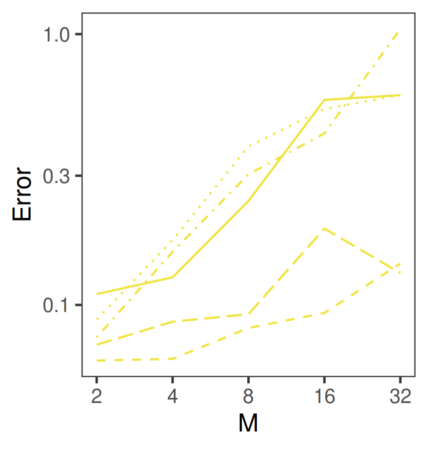
(f)

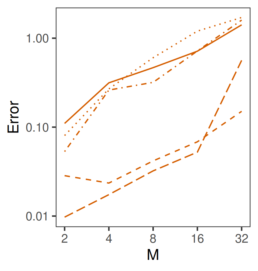
(g)

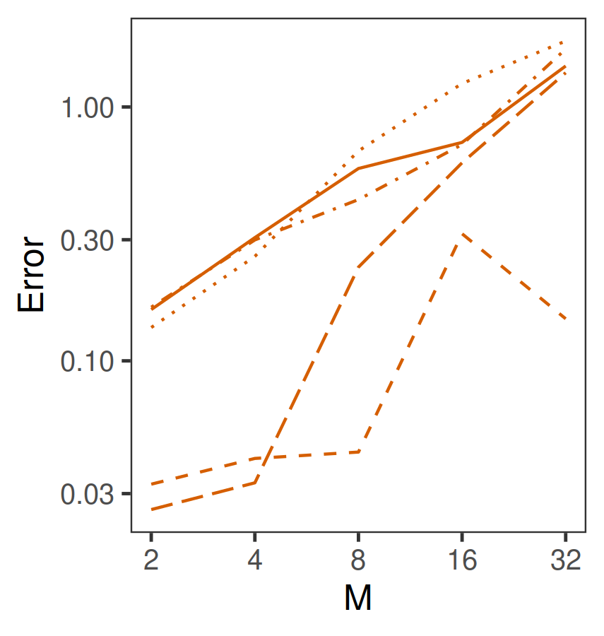
(h)

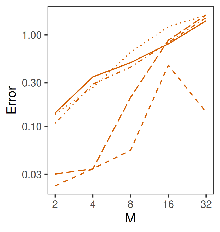
(i)

Figure 15: Posterior approximation comparisons in the logistic regression example of Section 3.3.2. The error in estimating (a)(d)(g) the posterior mean, (b)(e)(h) the 2.5% quantiles of the marginals of the posterior, (c)(f)(i) the 97.5% quantiles of the marginals of the posterior.

Figure 15 shows results for the LEMIE estimators only using all types of Laplace samples and none. We find that Laplace samples are beneficial to performance, but only those of type 1; including type 2 and type 3 Laplace samples does not seem to help and may make performance worse. LEMIE1 does not benefit much from adding Laplace samples of any type.

Figure 13b plots the error in estimating $\theta$ for all LEMIE results and in all $M$ simulations against the ESS and $\hat{{k}}$ diagnostics. In these examples, ESS and $\hat{{k}}$ appear to be useful predictors of performance.

4 Discussion and future work

We have introduced new methodology for estimating posterior expectations when data are partitioned, the Laplace enriched multiple importance estimator (LEMIE), which has three variants defined by different importance weighting schemes. Our method works with parallel sampling from local posteriors using any unbiased sampling algorithm and weights the samples obtained for use in Monte Carlo estimators. This is accomplished with new importance weighting schemes that allow for unnormalised proposal and posterior densities.

The performance of the LEMIE estimators in terms of KL divergence and error in estimating the posterior mean and tail quantiles appears to be generally good, almost always better than naive pooling of samples and sometimes better than CMC (Scott et al., (2016)) or DPE (Neiswanger et al., (2013)). It seems to be particularly good relative to these methods in small data, non-normal examples, as seen in the results with the beta-Bernoulli model in Section 3.1, estimation of the $\Sigma$ marginal of the posterior in the MVN example of Section 3.2 and the logistic regression example of Section 3.3.1.

The larger logistic example of Section 3.3.2 poses a tougher challenge for LEMIE, but the methods still do no worse than some of the other methods, and for large $M$ become competitive. This is remarkable for importance sampling-based methods used in a 50 dimensional parameter space given the curse of dimensionality. This seems to be thanks to including samples from the Laplace approximation of type 1 (Section 2.3.1). We have seen that a small number of Laplace samples of the right type, in particular type 1, can improve LEMIE a lot in complex examples. This is likely because the approximation is closer to the posterior than any of the local posteriors. The type 1 Laplace approximation is very similar to CMC2 (and the PDPE of Neiswanger et al., (2013)), so this is unsurprisingly good in normal examples or examples with large $n$. However, we have also seen that further improvements cannot be easily obtained by increasing the number of Laplace samples.

In our methods, any prior distribution can be used, unlike in some other methods such as CMC or DPE, which need to use a $\nicefrac{{1}}{{M}}^{\textrm{{th}}}$ power of the prior p.d.f. for the local sampling. This often entails a compromise in the form or parameterisation of the prior used, as we saw in examples in Sections 3.1 and 3.2. Incorrectly specified priors may not be an issue in big data situations (CMC and DPE are designed with big data applications in mind), since the influence of the prior on the posterior diminishes with $n$, but it may well be consequential in those scenarios with restrictions on data sharing where $n$ is not very large. It is not an issue when the prior is uninformative, but uninformative priors can be hard to interpret or lead to unstable estimates (Gelman et al., (2008)).

Having useful performance diagnostics - ESS and $\hat{{k}}$ - is another advantage of our methods. There are several variants of LEMIE to consider, including the Laplace approximation options, and some may work better than others in particular situations. These diagnostics can be useful in identifying which one is likely to perform better when there is no other means of calibration. Whilst we have some empirical evidence that the ESS is a useful diagnostic, it does not carry any guarantees. It is also based on two approximations of the estimator variance using the delta method, the second in particular having a non-negligible error term (see Appendix A.3). There are other issues in the ESS, discussed in Elvira et al., (2018), who also suggest some alternatives that we could use.

There are ways to estimate an ESS for the other methods, for instance the multivariate ESS for MCMC of Vats et al., (2019). This would not permit comparisons across methods, including LEMIE, to predict relative performance because the methods have different biases and the ESS is related to the variance of the estimators and not the bias.

One limitation of our methods is on how large we can make $M$. We found in the logistic regression examples of Section 3.3 that for a given number of samples from each local posterior, $\bar{N}$, there is an $M$ large enough that the necessary pooling and weighting operations on the master node of the $\bar{N}M$ samples may exceed the available memory resources. To get around this it may be possible to cap the number of samples drawn by each worker, but this may not be possible if the local MCMC samplers have not converged by that point, or to discard samples, although this will have a detrimental effect on the estimator variance.

We think it is likely that a random partition of the data is better for our methods than a non-random partition, or heterogeneous data, because that would make the local posteriors less likely to be good approximations to the posterior, as required for importance sampling to work well. This is a limitation for applications with real data if the data partition cannot be controlled. We did see in Section 3.1 that the methods perform well with heterogeneous data in a simple, 1 dimensional example; however, we are yet to investigate the impact of heterogeneous data in more complex examples.

In future work, it would be interesting to compare performance against methods outside of Scott et al., (2016) and Neiswanger et al., (2015), particularly methods which approach the problem in a different way such as Xu et al., (2014), Jordan et al., (2018), Nemeth and Sherlock, (2018), Park et al., (2020) and Rendell et al., (2020), and identify situations where one may perform better than another or where methods may complement each other. Our methods apply at the sample collection stage. This means they could be used in conjunction with some other methods, notably those of Xu et al., (2014) or Nemeth and Sherlock, (2018), in the latter case using our multiple importance weighting schemes in place of theirs. This may result in estimators that perform better in higher dimensions than either method on its own.

Another idea for improving our methods is to employ the importance weight smoothing used in the Pareto smoothed importance sampling (PSIS) of Vehtari et al., (2015). This would apply after computing the weights of type 1, 2 or 3 from Section 2.2. We have already investigated the use of $\hat{{k}}$ from the PSIS algorithm as a diagnostic (Section 2.4.2). Vehtari et al., (2015) find that importance estimator performance can be improved with PSIS when $\hat{{k}}<0.7$. This is something to explore in future work.

The simulation studies used in Section 3 to evaluate the performance of our methods are limited in scope. In order to better understand the strengths and limitations of our methods, experiments should be conducted on more complex models such as hierarchical models, large data sets and especially with real data. It would also be valuable to investigate performance under different conditions, such as non-random partitions of heterogeneous data, i.e. different data distributions in each node, multimodal posterior distributions, and the choice of MCMC algorithm employed for local posterior sampling.

Appendix A Derivations

A.1 Asymptotic results

A.1.1 Asymptotic unbiasedness of self-normalised importance sampling

Equation 11 is derived as

$$\lim_{N_{j}\to\infty}\frac{1}{N_{j}}\sum_{h=1}^{N_{j}}\tilde{w}_{j}\left(\theta_{j,h}\right) = \mathbb{{E}}_{\pi_{j}}\left[\tilde{w}_{j}\left(\theta\right)\right]$$ (81)

$$= \frac{Z_{\pi}}{Z_{j}}\int w_{j}\left(\theta\right)\pi_{j}\left(\theta\mid\mathbf{x}_{j}\right)\mathrm{{d}}\theta$$

$$= \frac{Z_{\pi}}{Z_{j}}\int\pi\left(\theta\mid x_{1:n}\right)\mathrm{{d}}\theta$$

$$= \frac{Z_{\pi}}{Z_{j}},$$

with the first line due to the strong law of large numbers. The importance estimator in Equation 10 of $\mathbb{{E}}_{\pi}\left[f\left(\theta\right)\right]$ has zero bias in the limit of $N_{j}\to\infty$ because

$$\lim_{N\to\infty}\tilde{\mu}_{j} = \lim_{N\to\infty}\frac{\frac{1}{N_{j}}\sum_{h=1}^{N_{j}}\tilde{w}_{j}\left(\theta_{h}\right)f\left(\theta_{h}\right)}{\frac{1}{N_{j}}\sum_{h=1}^{N_{j}}\tilde{w}_{j}\left(\theta_{h}\right)}$$ (82)

$$= \frac{\mathbb{{E}}_{\pi_{j}}\left[\tilde{w}_{j}\left(\theta\right)f\left(\theta\right)\right]}{\mathbb{{E}}_{\pi_{j}}\left[\tilde{w}_{j}\left(\theta\right)\right]}$$

$$= \mathbb{{E}}_{\pi_{j}}\left[\frac{Z_{j}}{Z_{\pi}}\tilde{w}_{j}\left(\theta\right)f\left(\theta\right)\right]$$ (83)

$$= \mathbb{{E}}_{\pi_{j}}\left[w_{j}\left(\theta\right)f\left(\theta\right)\right]$$ (84)

$$= \mathbb{{E}}_{\pi}\left[f\left(\theta\right)\right],$$ (85)

in which line 82 holds almost surely by the strong law of large numbers, line 83 is by Equation 11 and line 85 is by Equation 7.

A.1.2 Asymptotic unbiasedness of MIE2

The MIE2 estimator, Equation 26, has limit

$$\lim_{N_{1},\ldots,N_{M}\to\infty}\tilde{\mu}^{\textrm{{MIE2}}} = \lim_{N_{1},\ldots,N_{M}\to\infty}\frac{1}{N}\sum_{j=1}^{M}\sum_{h=1}^{N_{j}}\frac{\pi\left(\theta_{j,h}\mid x_{1:n}\right)f\left(\theta_{j,h}\right)}{\frac{1}{N}\sum_{k=1}^{M}N_{k}\frac{Z_{k}}{Z_{\pi}}\hat{c}_{k}\pi_{k}\left(\theta_{j,h}\mid\mathbf{x}_{k}\right)}$$ (86)

$$= \lim_{N_{1},\ldots,N_{M}\to\infty}\frac{1}{N}\sum_{j=1}^{M}\sum_{h=1}^{N_{j}}\pi\left(\theta_{j,h}\mid x_{1:n}\right)f\left(\theta_{j,h}\right)$$

$$\times\frac{1}{\lim_{N_{1},\ldots,N_{M}\to\infty}\frac{1}{N}\sum_{k=1}^{M}N_{k}\frac{Z_{k}}{Z_{\pi}}\hat{c}_{k}\pi_{k}\left(\theta_{j,h}\mid\mathbf{x}_{k}\right)}$$

$$= \lim_{N_{1},\ldots,N_{M}\to\infty}\frac{1}{N}\sum_{j=1}^{M}\sum_{h=1}^{N_{j}}\frac{\pi\left(\theta_{j,h}\mid x_{1:n}\right)f\left(\theta_{j,h}\right)}{\phi\left(\theta_{j,h}\right)}$$ (87)

$$= \mathbb{{E}}\left[w_{\phi}\left(\theta\right)f\left(\theta\right)\right]$$ (88)

$$= \mathbb{{E}}_{\pi}\left[f\left(\theta\right)\right].$$ (89)

Line 86 is possible because the limit of the denominator is not zero, line 87 evaluates the limit for the denominator by replacing $\hat{c}_{k}$ with its estimand $\frac{Z_{\pi}}{Z_{k}}$, line 88 is by the strong law of large numbers and line 89 follows from Equation 7.

A.2 Bias and variance of estimators

A.2.1 Finite-sample bias of MIE2

The MIE2 estimator without self-normalising can be written as

$$\tilde{\mu}^{\textrm{{MIE2}}}=\sum_{j=1}^{M}\sum_{h=1}^{N_{j}}\frac{\pi\left(\theta_{j,h}\mid x_{1:n}\right)f\left(\theta_{j,h}\right)}{\frac{1}{N}\sum_{k=1}^{M}N_{k}\bar{\hat{c}}_{k}\pi_{k}\left(\theta_{j,h}\mid\mathbf{x}_{k}\right)}.$$ (90)

where

$$\bar{\hat{c}}_{k}:=\frac{1}{N_{k}}\sum_{i=1}^{N_{k}}\frac{\pi\left(\theta_{k,i}\mid x_{1:n}\right)}{\pi_{k}\left(\theta_{k,i}\mid\mathbf{x}_{k}\right)}.$$ (91)

The bias can be attributed to the Monte Carlo average Equation 91, as can be seen in Equation 89. Equation 91 converges to 1 in the limit $N_{k}\to\infty$. Write the denominator of the weights as

$$\tilde{\phi}\left(\theta\right) := \frac{1}{N}\sum_{k=1}^{M}N_{k}\bar{\hat{c}}_{k}\pi_{k}\left(\theta\mid\mathbf{x}_{k}\right)$$ (92)

$$= \frac{1}{N}\sum_{k=1}^{M}N_{k}\left[1+\varepsilon_{k}\right]\pi_{k}\left(\theta\mid\mathbf{x}_{k}\right)$$

$$= \phi\left(\theta\right)+\varepsilon\left(\theta\right),$$

where $\varepsilon_{k}\sim\textrm{{N}}\left(0,\frac{\sigma_{k}^{2}}{N_{k}}\right)$ by the central limit theorem with

$$\sigma_{k}^{2}:=\textrm{{Var}}\left(\frac{\pi\left(\theta\mid x_{1:n}\right)}{\pi_{k}\left(\theta\mid\mathbf{x}_{k}\right)}\right)$$ (93)

and

$$\varepsilon\left(\theta\right):=\frac{1}{N}\sum_{k=1}^{M}N_{k}\varepsilon_{k}\pi_{k}\left(\theta\mid\mathbf{x}_{k}\right).$$ (94)

Then we can write

$$\mathbb{{E}}\left[\tilde{\mu}^{\textrm{{MIE2}}}\right] = \mathbb{{E}}\left[\frac{\frac{1}{N}\sum_{j=1}^{M}\sum_{h=1}^{N_{j}}\pi\left(\theta\mid x_{1:n}\right)f\left(\theta\right)}{\phi\left(\theta\right)+\varepsilon\left(\theta\right)}\right],$$ (95)

which we can estimate using the delta method. Let

$$\bar{V} := \frac{1}{N}\sum_{j=1}^{M}\sum_{h=1}^{N_{j}}\pi\left(\theta\mid x_{1:n}\right)f\left(\theta\right),$$

$$U := \phi\left(\theta\right)+\varepsilon\left(\theta\right),$$ (96)

then the expectation of the Taylor series of $g\left(U,\bar{V}\right)=\frac{\bar{V}}{U}$ truncated at the 2nd order term (required to estimate bias, Owen, (2013)) gives us

$$\mathbb{{E}}\left[\tilde{\mu}^{\textrm{{MIE2}}}\right] \approx g\left(\mu_{U},\mu_{V}\right)+\frac{1}{2}\left[\sigma_{U}^{2}\frac{\partial^{2}}{\partial U^{2}}g\left(\mu_{U},\mu_{V}\right)\right.$$ (97)

$$+\frac{1}{N}\sigma_{V}^{2}\frac{\partial^{2}}{\partial V^{2}}g\left(\mu_{U},\mu_{V}\right)$$

$$\left.+2\textrm{{Cov}}\left(U,V\right)\frac{\partial^{2}}{\partial U\partial V}g\left(\mu_{U},\mu_{V}\right)\right],$$

where $\mu_{U},\sigma_{U}^{2}$ and $\mu_{V},\sigma_{V}^{2}$ are the expectations and variances of $U$ and $V$ respectively and $\textrm{{Cov}}\left(U,V\right)$ is their covariance. Since $\mathbb{{E}}\left[\varepsilon\left(\theta\right)\right]=0$ and $\varepsilon_{k}$ is independent of $\theta$, Equation 97 can be simplified to

$$\mathbb{{E}}\left[\tilde{\mu}^{\textrm{{MIE2}}}\right] \approx \frac{\mu_{V}}{\mu_{U}}+\frac{1}{\mu_{U}^{2}}\left(\textrm{{Var}}\left(\phi\left(\theta\right)\right)\frac{\mu_{V}}{\mu_{U}}-\mathrm{{Cov}}\left(U,V\right)\right)$$ (99)

$$+\frac{1}{\mu_{U}^{2}}\textrm{{Var}}\left(\varepsilon\left(\theta\right)\right)\frac{\mu_{V}}{\mu_{U}}.$$

If we had applied the delta method to the estimator using weights Equation 19 we would have gotten line 99 with the same values of $\mu_{U},\mu_{V}$ and $\mathrm{{Cov}}\left(U,V\right)$. But we know that that estimator is unbiased, so

$$\mathbb{{E}}\left[\tilde{\mu}^{\textrm{{MIE2}}}\right] \approx \mathbb{{E}}_{\pi}\left[f\left(\theta\right)\right]+\frac{1}{\mu_{U}^{2}}\textrm{{Var}}\left(\varepsilon\left(\theta\right)\right)\frac{\mu_{V}}{\mu_{U}}$$ (100)

$$= \mathbb{{E}}_{\pi}\left[f\left(\theta\right)\right]+\frac{1}{\mathbb{{E}}\left[\phi\left(\theta\right)\right]^{2}}\textrm{{Var}}\left(\varepsilon\left(\theta\right)\right)\frac{\mathbb{{E}}\left[\pi\left(\theta\mid x_{1:n}\right)f\left(\theta\right)\right]}{\mathbb{{E}}\left[\phi\left(\theta\right)\right]}$$

where

$$\textrm{{Var}}\left(\varepsilon\left(\theta\right)\right) = \frac{1}{N^{2}}\sum_{k=1}^{M}N_{k}^{2}\textrm{{Var}}\left(\varepsilon_{k}\pi_{k}\left(\theta_{j,h}\mid\mathbf{x}_{k}\right)\right)$$ (101)

$$= \frac{1}{N^{2}}\sum_{k=1}^{M}N_{k}^{2}\textrm{{Var}}\left(\varepsilon_{k}\right)\mathbb{{E}}\left[\pi_{k}\left(\theta_{j,h}\mid\mathbf{x}_{k}\right)^{2}\right].$$

A.2.2 Variance of MIE2

Using the notation of Section A.2.1 we have

$$\textrm{{Var}}\left(\tilde{\mu}^{\textrm{{MIE2}}}\right) \approx \frac{\mu_{V}^{2}}{\mu_{U}^{4}}\sigma_{U}^{2}+\frac{1}{N}\frac{1}{\mu_{U}^{2}}\sigma_{V}^{2}-\frac{\mu_{V}}{\mu_{U}^{3}}\textrm{{Cov}}\left(U,V\right)$$ (102)

$$= \frac{1}{\mu_{U}^{2}}\left(\frac{\mu_{V}^{2}}{\mu_{U}^{2}}\sigma_{U}^{2}+\frac{1}{N}\sigma_{V}^{2}-\frac{\mu_{V}}{\mu_{U}}\textrm{{Cov}}\left(U,V\right)\right)$$

$$= \frac{1}{\mu_{U}^{2}}\left(\frac{\mu_{V}^{2}}{\mu_{U}^{2}}\textrm{{Var}}\left(\phi\left(\theta\right)\right)+\frac{1}{N}\sigma_{V}^{2}-\frac{\mu_{V}}{\mu_{U}}\textrm{{Cov}}\left(U,V\right)\right)$$

$$+\frac{1}{\mu_{U}^{2}}\frac{\mu_{V}^{2}}{\mu_{U}^{2}}\textrm{{Var}}\left(\varepsilon\left(\theta\right)\right).$$

Following the same reasoning as above, the $\frac{1}{\mu_{U}^{2}}\frac{\mu_{V}^{2}}{\mu_{U}^{2}}\textrm{{Var}}\left(\varepsilon\left(\theta\right)\right)$ term is the additional variance due to the Monte Carlo estimate of the ratio of normalising constants. The rest is the variance of the normalised estimator.

A.3 ESS of MIE1

The approximate ESS for MIE1, Equation 52, is derived from an additional application of the delta method to Equation 16. We follow the reasoning of Kong, (1992). Equation 16 can be written as

$$\mathrm{{Var}}\left(\tilde{\mu}^{\textrm{{MIE1}}}\right) \approx \sum_{j=1}^{M}\frac{N_{j}}{N^{2}}\left(\textrm{{Var}}\left(w_{j}\left(\theta\right)\right)\mathbb{{E}}_{\pi}^{2}\left[f\left(\theta\right)\right]+\textrm{{Var}}\left(w_{j}\left(\theta\right)f\left(\theta\right)\right)\right.$$ (103)

$$\left.-2\textrm{{Cov}}\left(w_{j}\left(\theta\right),w_{j}\left(\theta\right)f\left(\theta\right)\right)\mathbb{{E}}_{\pi}\left[f\left(\theta\right)\right]\right).$$

The delta method is used to approximate the $\mathbb{{E}}\left[w_{j}\left(\theta\right)^{2}f\left(\theta\right)^{2}\right]$ term in $\textrm{{Var}}\left(w_{j}\left(\theta\right)f\left(\theta\right)\right)$. This term is equal to $\mathbb{{E}}_{\pi}\left[w_{j}\left(\theta\right)f\left(\theta\right)^{2}\right]$. The Taylor expansion of $g^{\prime}\left(U,V\right):=UV^{2}$ evaluated at the expectation of $U$ and $V$ and truncated after the second order term leads to the approximation

$$\mathbb{{E}}_{\pi}\left[w_{j}\left(\theta\right)f\left(\theta\right)^{2}\right] \approx \mathbb{{E}}_{\pi}\left[w_{j}\left(\theta\right)\right]\mathbb{{E}}_{\pi}^{2}\left[f\left(\theta\right)\right]+\textrm{{Var}}_{\pi}\left(f\left(\theta\right)\right)\mathbb{{E}}_{\pi}\left[w_{j}\left(\theta\right)\right]$$ (104)

$$+2\textrm{{Cov}}_{\pi}\left(w_{j}\left(\theta\right),f\left(\theta\right)\right)\mathbb{{E}}_{\pi}\left[f\left(\theta\right)\right].$$

The error term of this “is not necessarily small”, according to Liu and Liu, (2001, , p36). Substituting into Equation 103 and simplifying leads us to

$$\mathrm{{Var}}\left(\tilde{\mu}^{\textrm{{MIE1}}}\right)\approx\sum_{j=1}^{M}\frac{N_{j}}{N^{2}}\textrm{{Var}}_{\pi}\left(f\left(\theta\right)\right)\left(\textrm{{Var}}\left(w_{j}\left(\theta\right)\right)+1\right).$$ (105)

This is rearranged to give $\textrm{{ESS}}_{1}$,

$$\frac{\textrm{{Var}}_{\pi}\left(f\left(\theta\right)\right)}{\mathrm{{Var}}\left(\tilde{\mu}^{\textrm{{MIE1}}}\right)} \approx \frac{1}{\sum_{j=1}^{M}\frac{N_{j}}{N^{2}}\mathbb{{E}}_{\pi}\left[w_{j}\left(\theta\right)^{2}\right]},$$ (106)

which is estimated as Equation 52.

A.4 Fractionated prior in MVN

The marginal prior density for $\Sigma$ is proportional to

$$\left|\Sigma\right|^{\frac{-\left(\nu+d+1\right)}{2}}\exp\left\{-\frac{1}{2}\mathrm{{tr}}\left(\Psi\Sigma^{-1}\right)\right\}.$$ (107)

For fractionation this must be raised to the $\nicefrac{{1}}{{M}}^{\textrm{{th}}}$ power, so to reparameterise we define $\nu^{*}$ such that

$$\nu^{*}+d+1=\frac{1}{M}\left(\nu+d+1\right)$$ (108)

and solve for $\nu^{*}$:

$$\nu^{*}=\frac{\nu}{M}-\frac{M-1}{M}d-\frac{M-1}{M}.$$ (109)

In the uninformative prior we put $\nu=0$. This implies that

$$\lim_{M\to\infty}\nu^{*}=-d-1.$$ (110)

We could therefore use $\nu^{*}=-d-1$ for a fractionated prior that is invariant with respect to $M$ and therefore can be used in all our simulations. This would be an improper prior for $\Sigma$, but the posterior distribution is proper under the following condition for positive integer $n$:

$$\nu^{*}+n >d-1$$

$$\implies -d-1+n >d-1$$

$$\implies n >2d.$$ (111)

This must also be the case for every local posterior, so if data are distributed evenly we must have $n$ such that $\left\lfloor\frac{n}{M}\right\rfloor>2d$.

Appendix B Semiparametric density product estimator (SDPE)

As explained in Section 2.5.2, the SDPE algorithm of Neiswanger et al., (2013) is similar to the NDPE algorithm but involves a KDE of $\frac{\pi_{j}\left(\theta\mid\mathbf{x}_{j}\right)}{\tilde{\varphi}_{j}\left(\theta\right)}$. The product of these $M$ KDE approximations and the normal approximations is a density product estimator of the posterior. Similarly to NDPE, this can be expressed as the mixture distribution

$$\hat{\pi}^{\mathrm{{SDPE}}}\left(\theta\right) := \frac{1}{\bar{N}^{M}}\prod_{j=1}^{M}\sum_{h=1}^{\bar{N}}\frac{\mathrm{{N}}_{p}\left(\theta\mid\theta_{j,h},bI_{p}\right)\mathrm{{N}}_{p}\left(\theta\mid\tilde{\mu}_{j},\tilde{\Sigma}_{j}\right)}{b^{p}\mathrm{{N}}_{p}\left(\theta_{j,h}\mid\tilde{\mu}_{j},\tilde{\Sigma}_{j}\right)}$$ (112)

$$\propto \sum_{h_{1}=1}^{\bar{N}}\cdots\sum_{h_{M}=1}^{\bar{N}}W\left(h_{1},\ldots,h_{M}\right)$$

$$\times\mathrm{{N}}_{p}\left(\theta\mid\mu\left(h_{1},\ldots,h_{M}\right),\Sigma\left(h_{1},\ldots,h_{M}\right)\right)$$

where

$$\Sigma\left(h_{1},\ldots,h_{M}\right):=\left(\frac{M}{b}I_{p}+\left(\Sigma^{*}\right)^{-1}\right)^{-1}$$ (113)

and

$$\mu\left(h_{1},\ldots,h_{M}\right):=\Sigma\left(h_{1},\ldots,h_{M}\right)\left(\frac{M}{b}I_{p}\bar{\theta}\left(h_{1},\ldots,h_{M}\right)+\mu^{*}\right),$$ (114)

with unnormalised weights

$$W\left(h_{1},\ldots,h_{M}\right):=\frac{w\left(h_{1},\ldots,h_{M}\right)\mathrm{\mathrm{{N}}_{p}}\left(\bar{\theta}\left(h_{1},\ldots,h_{M}\right)\mid\mu^{*},\Sigma^{*}\right)}{\prod_{j=1}^{M}\mathrm{{N}}_{p}\left(\theta_{j,h_{j}}\mid\tilde{\mu}_{j},\tilde{\Sigma}_{j}\right)}.$$ (115)

$\mu^{*}$ and $\Sigma^{*}$ are from Equations 60 and 59 respectively. A similar independent Metropolis-within-Gibbs algorithm is used to sample from the mixture distribution Equation 112 as described in Section 2.5.2.

Appendix C Gibbs sampler for logistic regression from Polson et al., (2013)

The algorithm of Polson et al., (2013) uses an augmented variable approach to generate samples from the posterior of $\theta$ conditional on data $x_{i},c_{i},y_{i}$ for $i=1,2,\ldots,n$ using Gibbs sampling without any approximations or Metropolis steps, making it computationally efficient. The likelihood is characterised as a scale mixture of normal distributions. The marginal distribution of the scale parameter is the Pólya-gamma distribution, which is constructed so that the full conditional distribution for $\theta$ with prior $\mathrm{{N}}_{p}\left(b,B\right)$ is also MVN.

The augmentation variables are $\omega_{i}>0$ for $i=1,2,\ldots,n$, and the Gibbs sampler consists of sampling iteratively from the full conditionals

$$\omega_{i}\mid x_{i},c_{i},y_{i},\theta \sim \mathrm{{PG}}\left(c_{i},x_{i}^{\intercal}\theta\right),i=1,2,\ldots,n,$$

$$\theta\mid x_{1:n},c_{1:n},y_{1:n},\omega_{1:n} \sim \mathrm{{N}}_{p}\left(m_{\omega},V_{\omega}\right)$$

where

$$V_{\omega} = \left(x_{1:n}^{\intercal}\Omega x_{1:n}+B^{-1}\right)^{-1},$$

$$m_{\omega} = V_{\omega}\left(x_{1:n}^{\intercal}\kappa+B^{-1}b\right),$$

in which $\Omega$ is the diagonal matrix with $\omega_{1:n}$ on the diagonal and $\kappa=\left(y_{1}-\frac{c_{1}}{2},\dots,y_{n}-\frac{c_{n}}{2}\right)$. $\mathrm{{PG}}\left(b,a\right)$ is the Pólya-gamma distribution, for details on which see Polson et al., (2013), who devise an efficient sampling algorithm implemented in R package BayesLogit (Polson et al., (2013)).

Appendix D Additional results

D.1 Multivariate normal studies

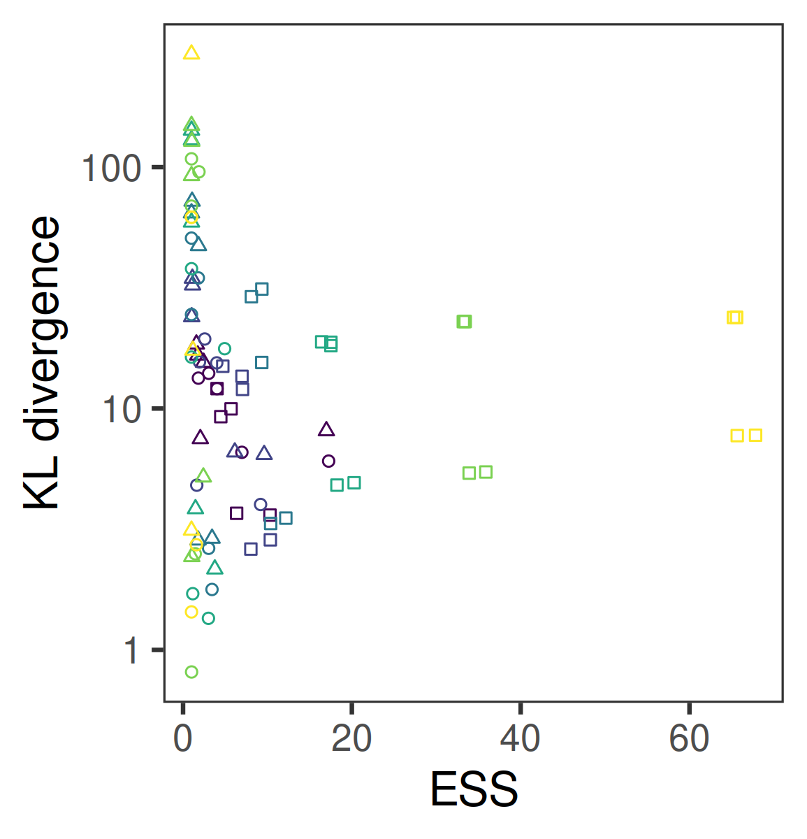
(a) KL divergence vs ESS.

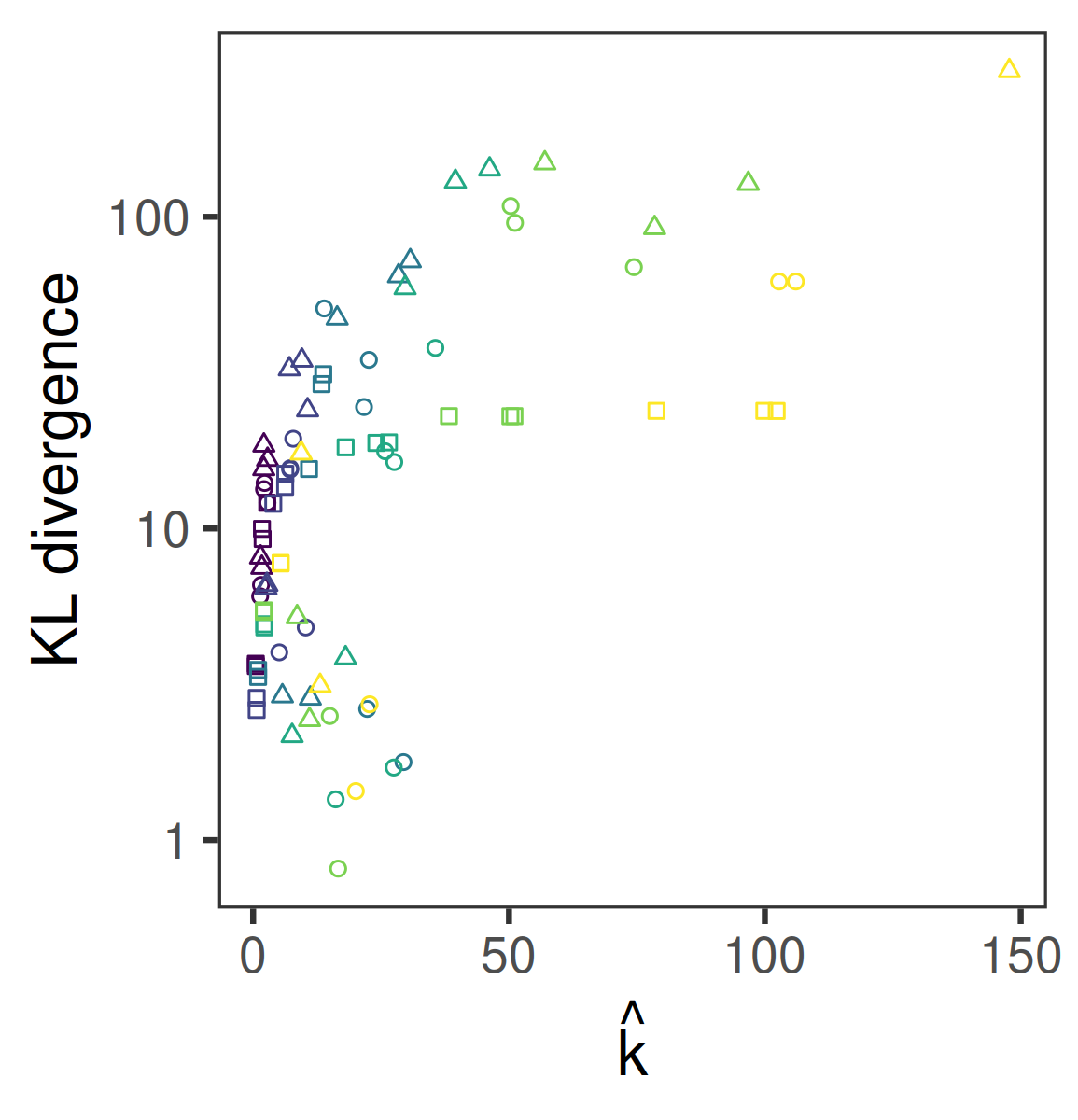
(b) KL divergence vs $\hat{{k}}$.

Figure 16: For the simulated examples of Section 3.2 with $d=8$ and $n=10,000$, KL divergences from the $\mu$ marginal of the posterior to the LEMIE approximations using the approach explained in Section 3 against the performance metrics of Section 2.4.

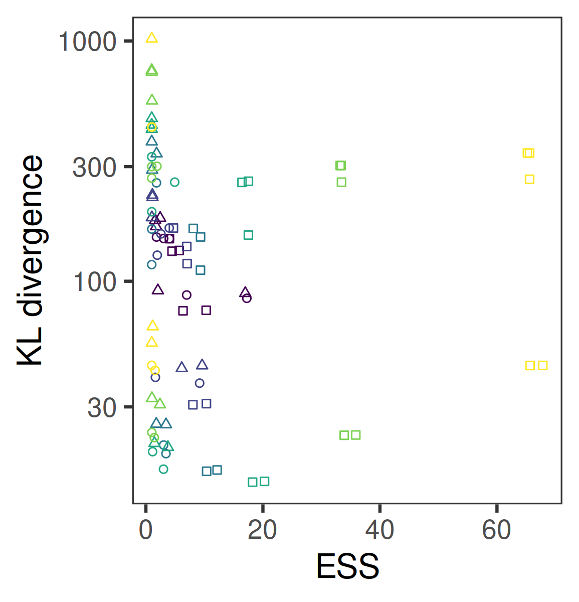
(a) KL divergence vs ESS.

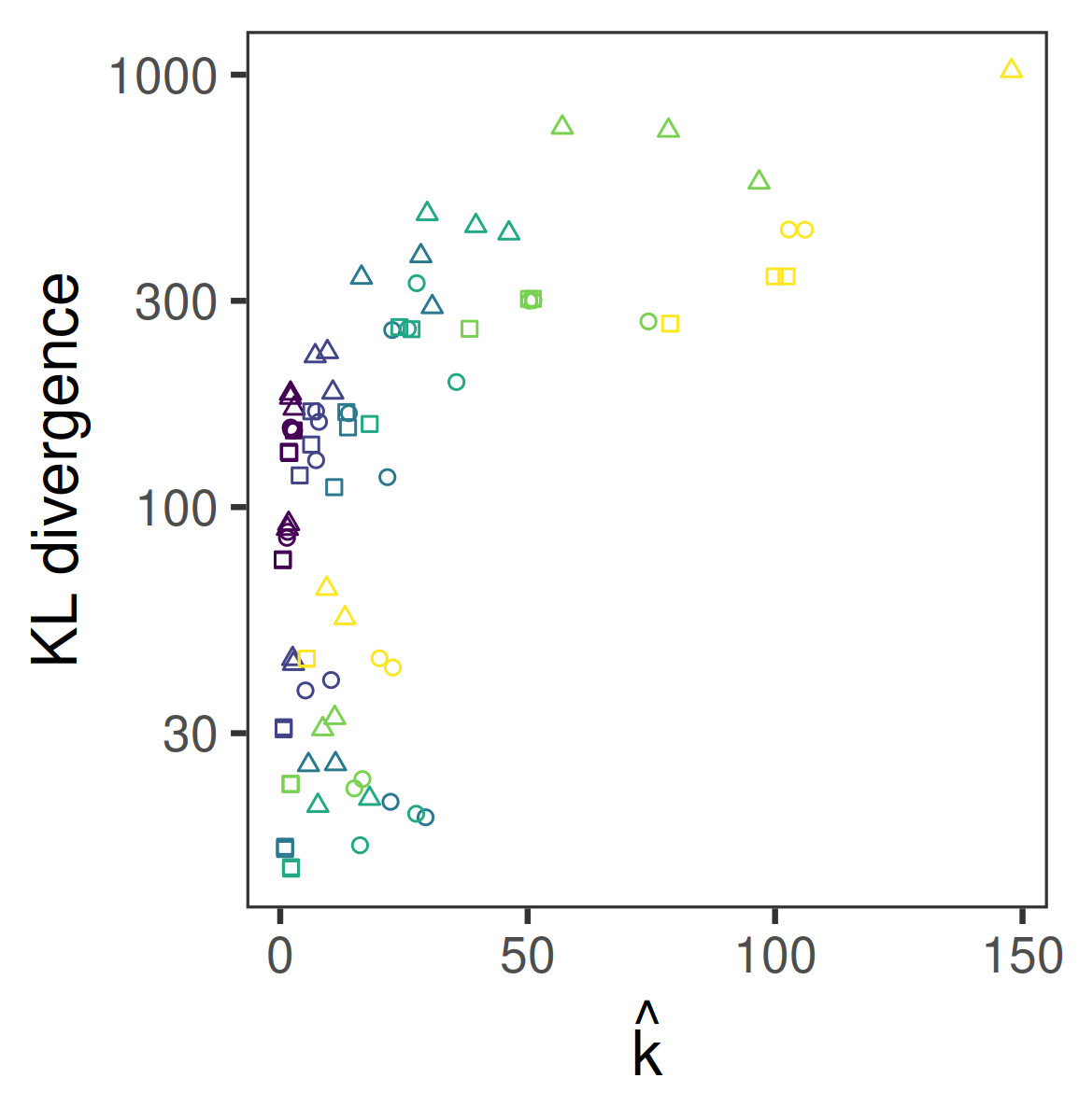
(b) KL divergence vs $\hat{{k}}$.

Figure 17: Similar to Figure 16 but of the KL divergences from the $\Sigma$ marginal of the posterior to the LEMIE approximations.

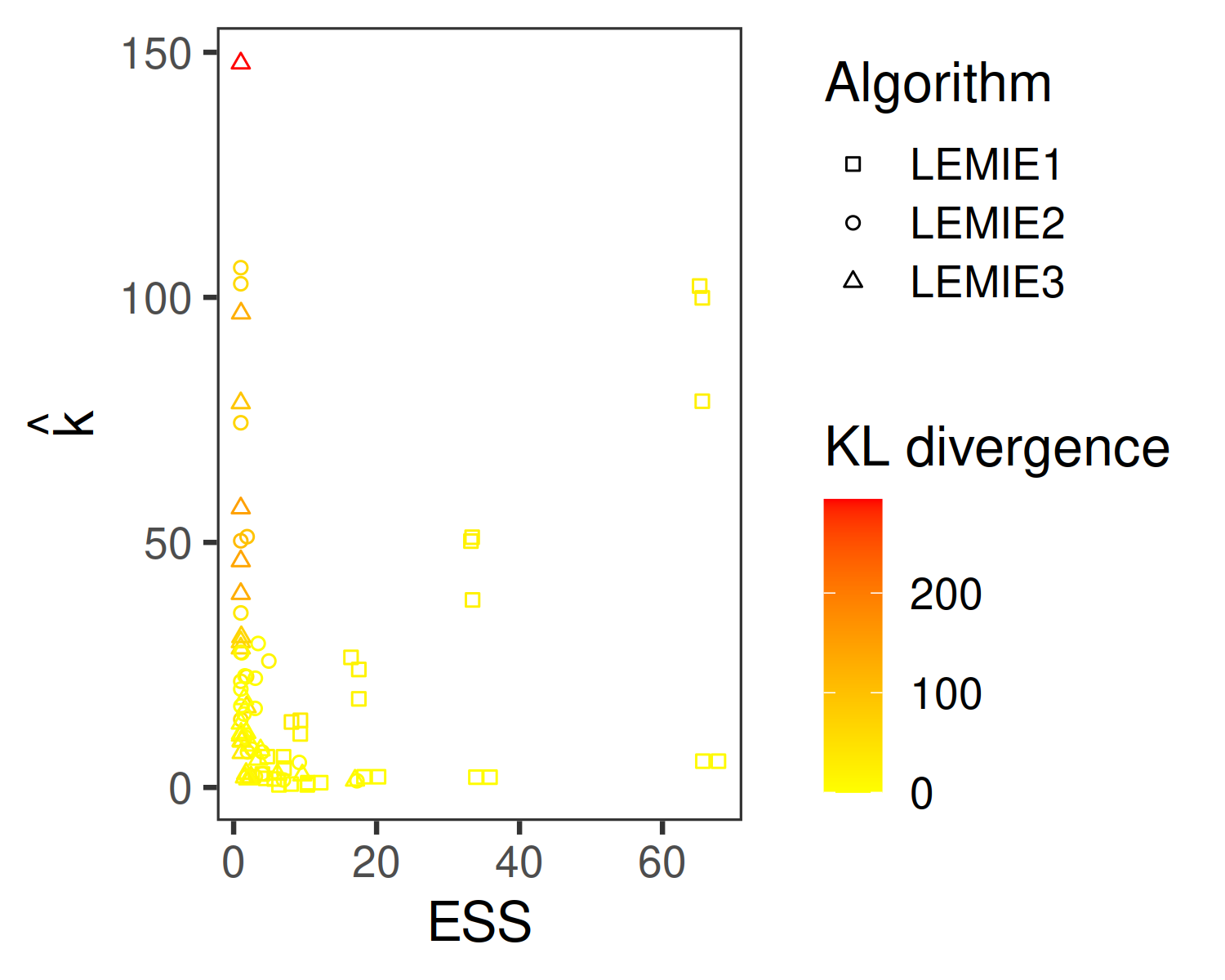
(a) Approximating the $\mu$ marginal of the posterior.

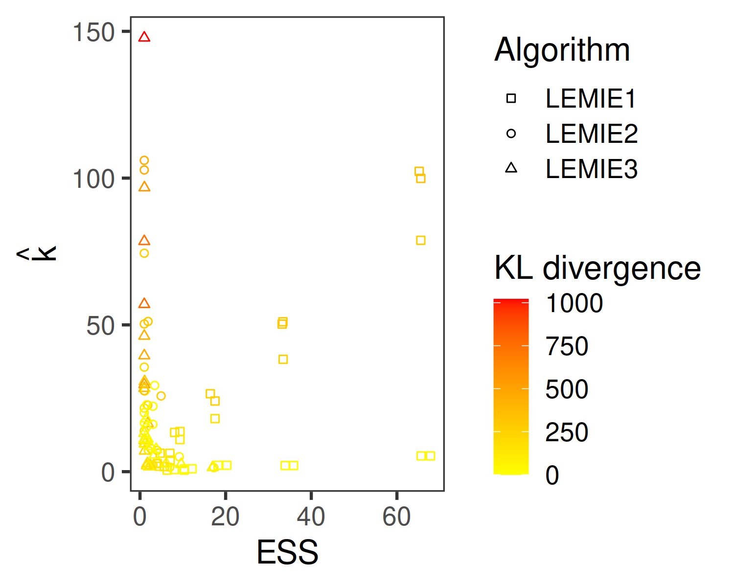
(b) Approximating the $\Sigma$ marginal of the posterior.

Figure 18: For the simulated examples of Section 3.2, KL divergences Equation 73 from the posterior to the LEMIE approximations using the approach explained in Section 3 against the performance metrics of Section 2.4.

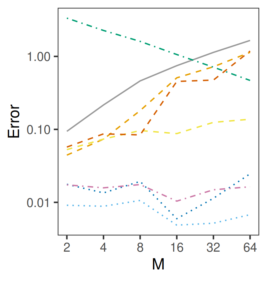
(a) Error in estimating the 2.5% quantiles of the $\mu$ marginal of the posterior.

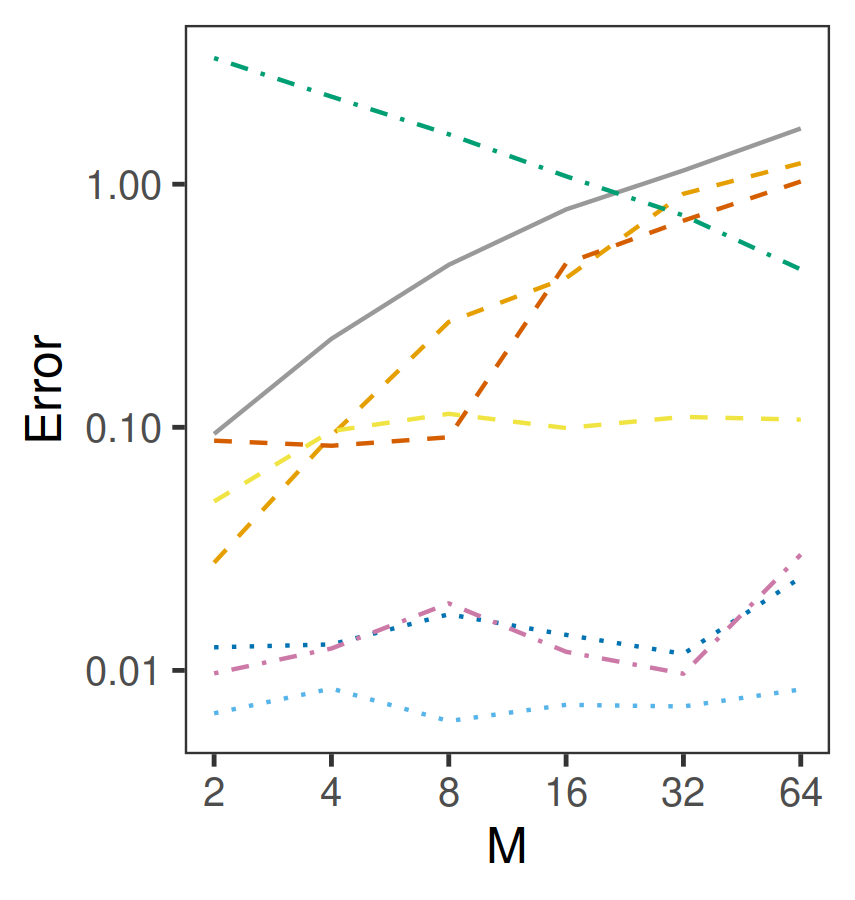
(b) Error in estimating the 97.5% quantiles of the $\mu$ marginal of the posterior.

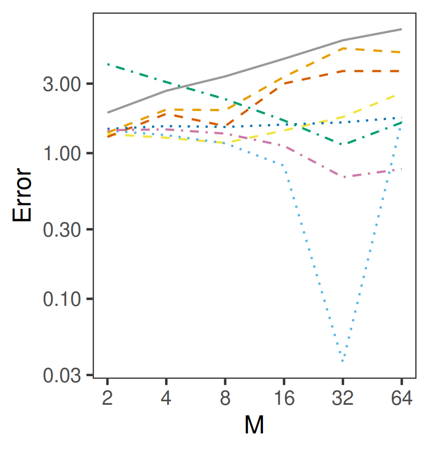
(c) Error in estimating the 2.5% quantiles of the $\Sigma$ marginal of the posterior.

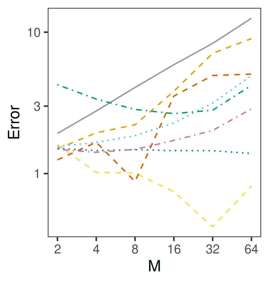
(d) Error in estimating the 97.5% quantiles of the $\Sigma$ marginal of the posterior.

Figure 19: Posterior approximation comparisons in the MVN example of Section 3.2 with $\mu$ and $\Sigma$ unknown, $d=8$ and $n=10,000$.

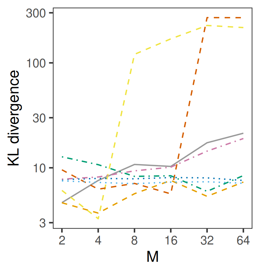
(a) KL divergence from the approximations to the posterior of $\mu$.

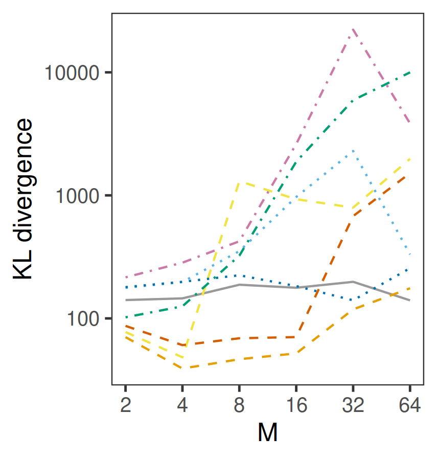
(b) KL divergence from the approximations to the posterior of $\Sigma$.

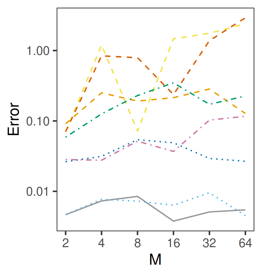
(c) Error in estimating the posterior mean of $\mu$.

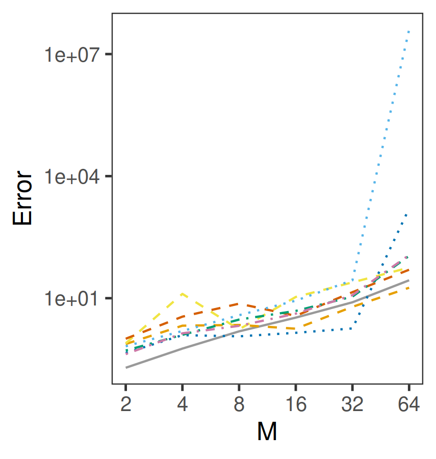
(d) Error in estimating the posterior mean of $\Sigma$.

Figure 20: Results similar to Figure 5 but with $d=8$ and $n=1,088$.

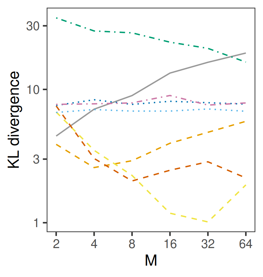
(a) KL divergence from the approximations to the posterior of $\mu$.

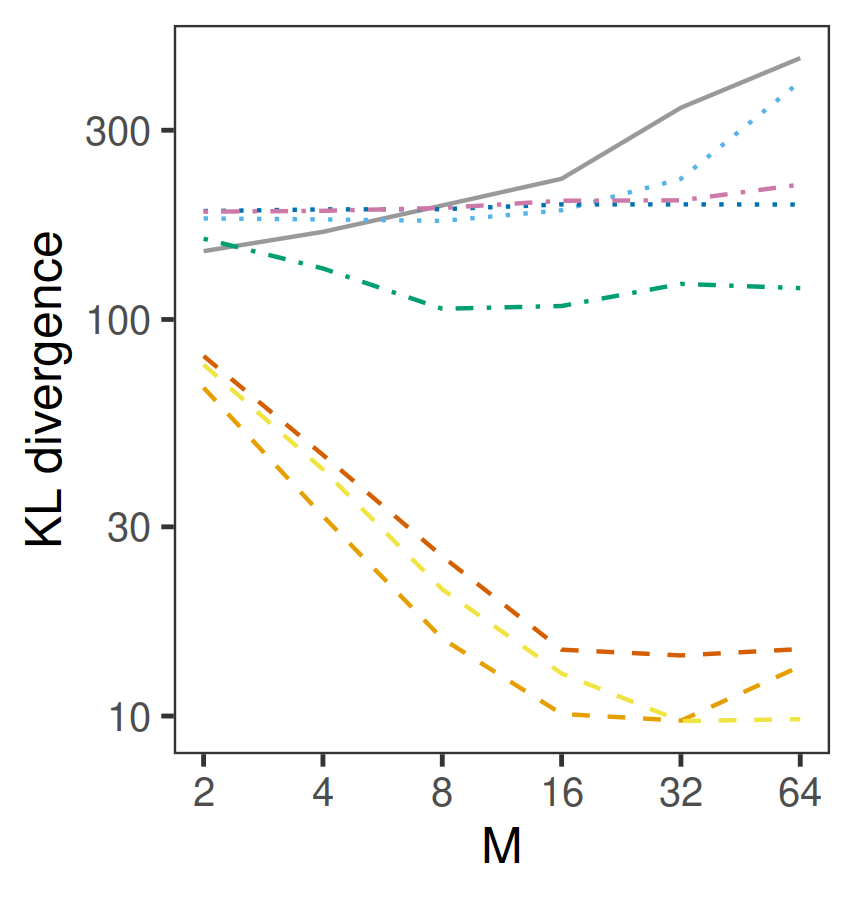
(b) KL divergence from the approximations to the posterior of $\Sigma$.

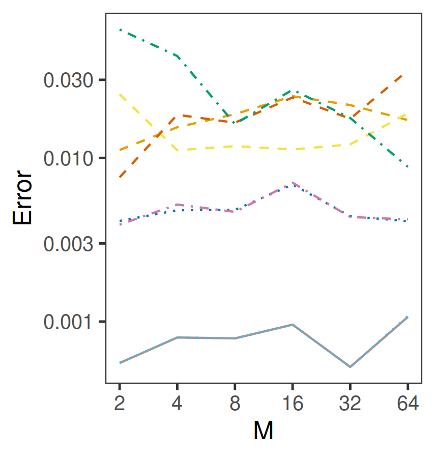
(c) Error in estimating the posterior mean of $\mu$.

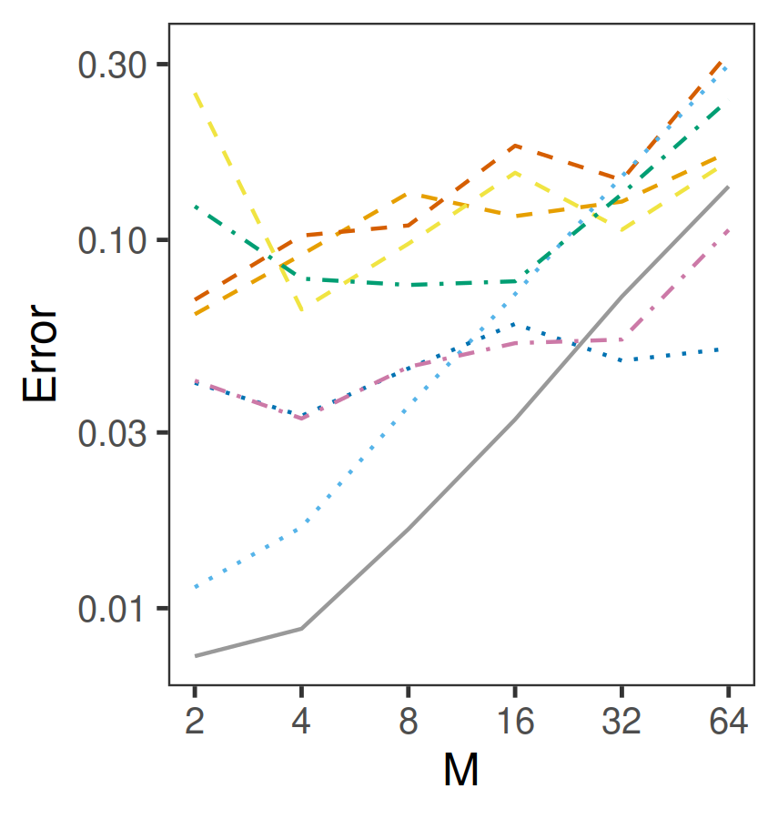
(d) Error in estimating the posterior mean of $\Sigma$.

Figure 21: Results similar to Figure 5 but with $d=8$ and $n=100,000$.

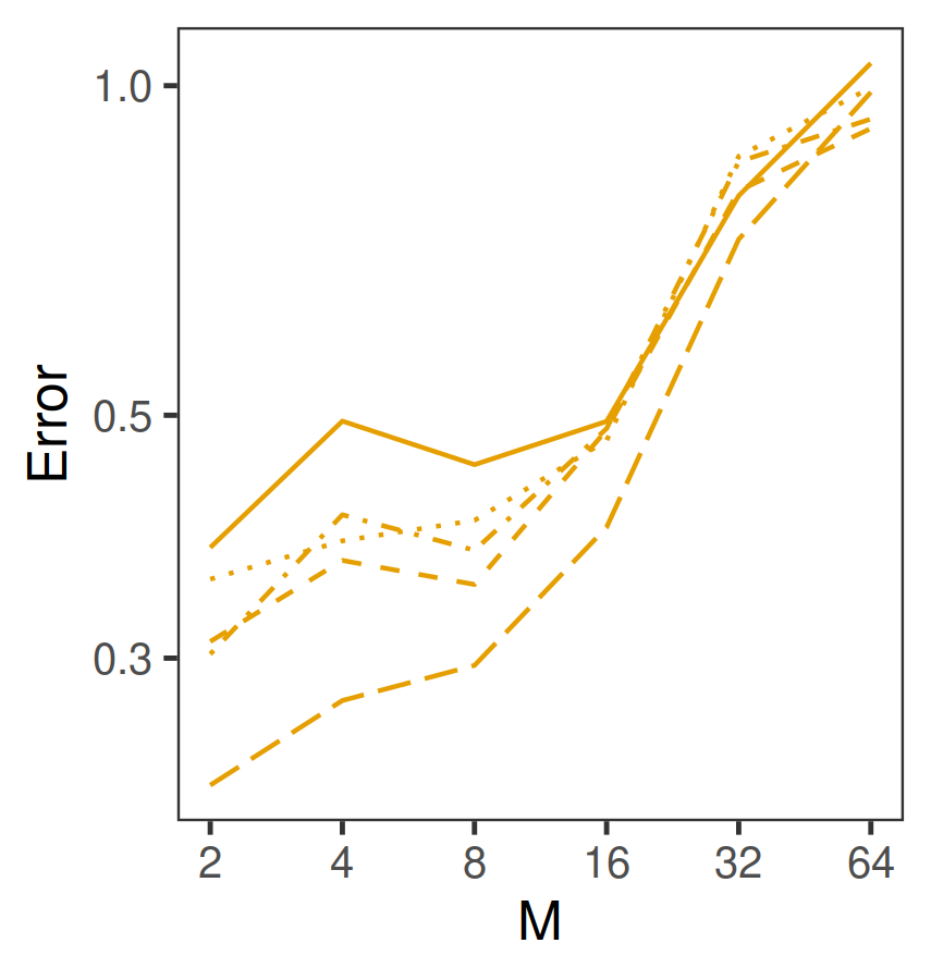
(a)

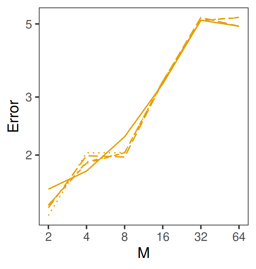
(b)

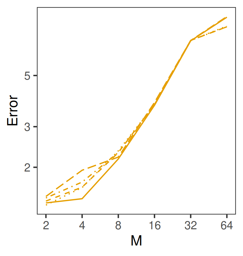
(c)

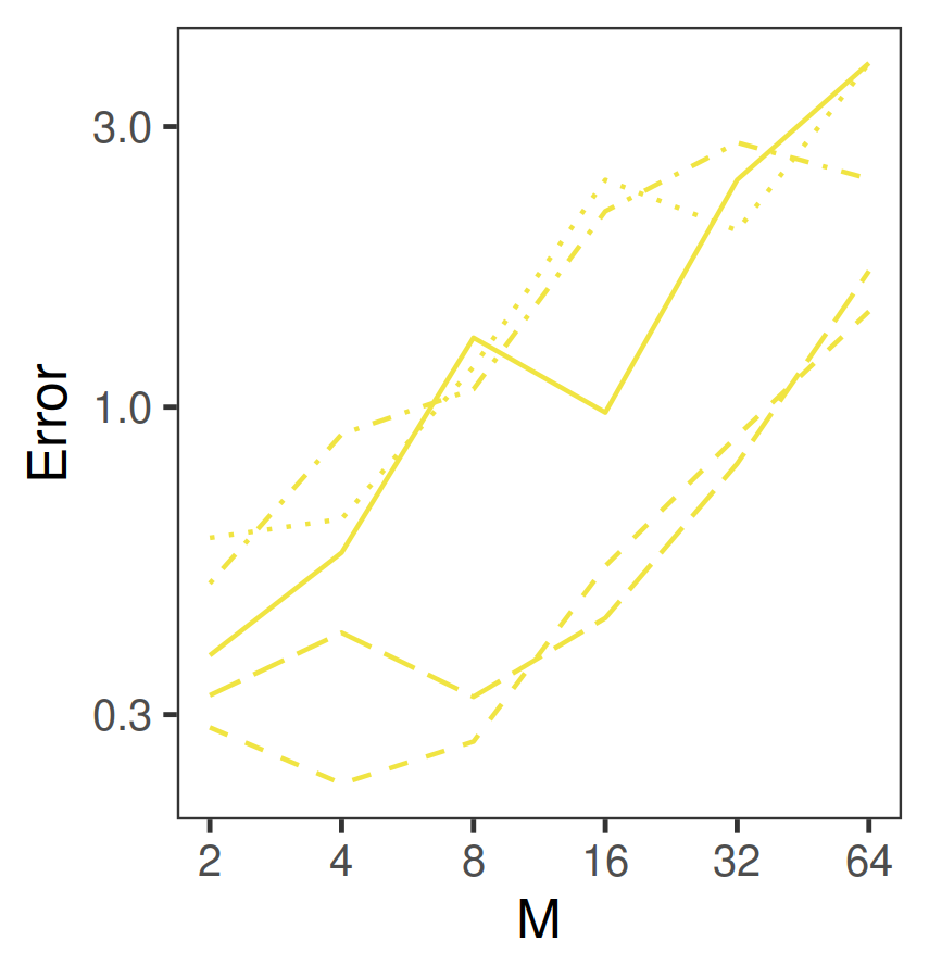
(d)

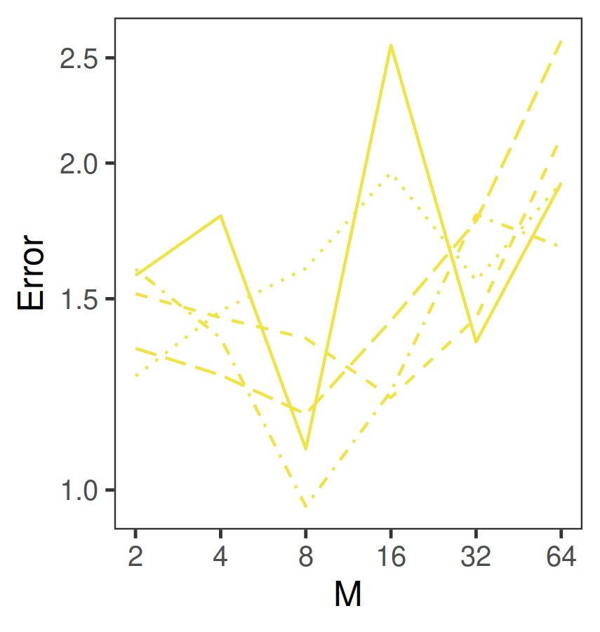
(e)

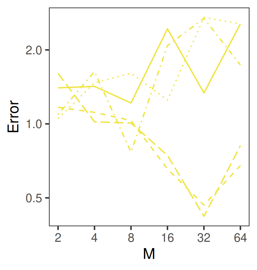
(f)

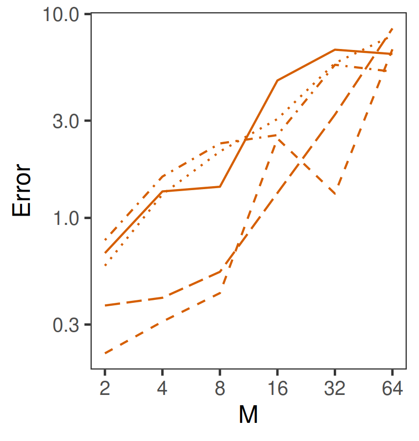
(g)

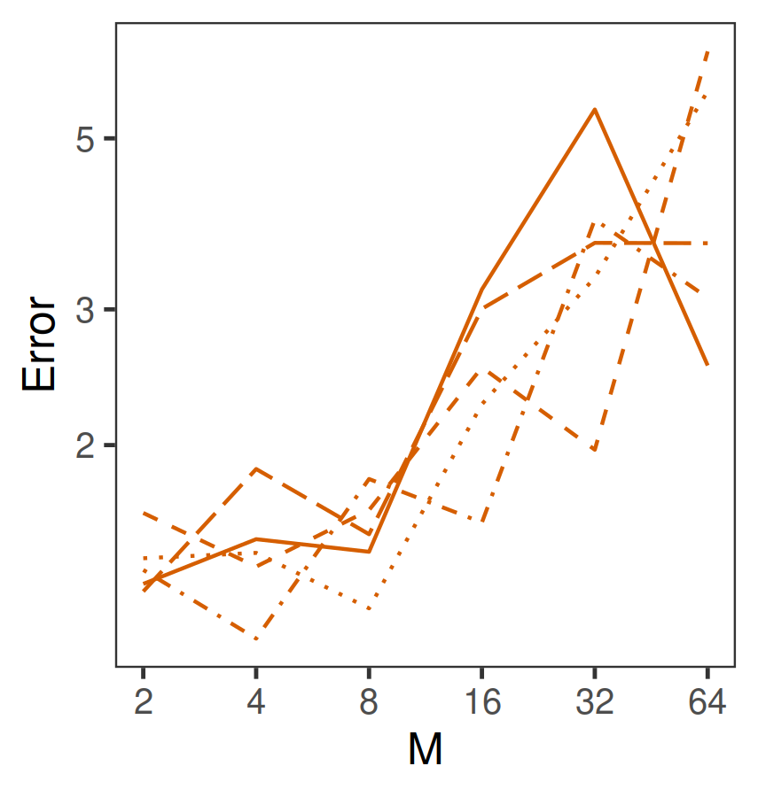
(h)

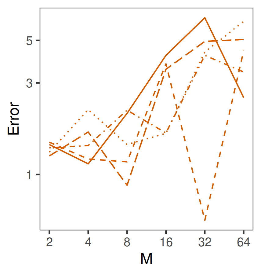
(i)

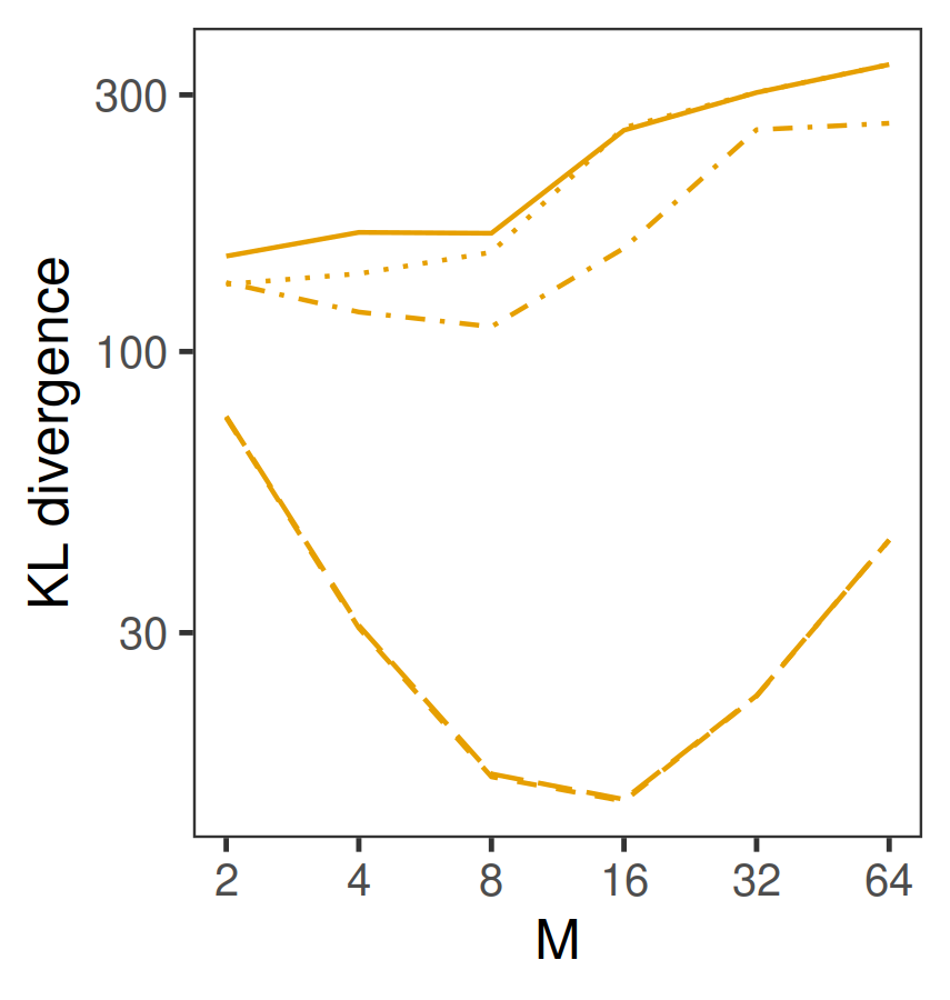
(j)

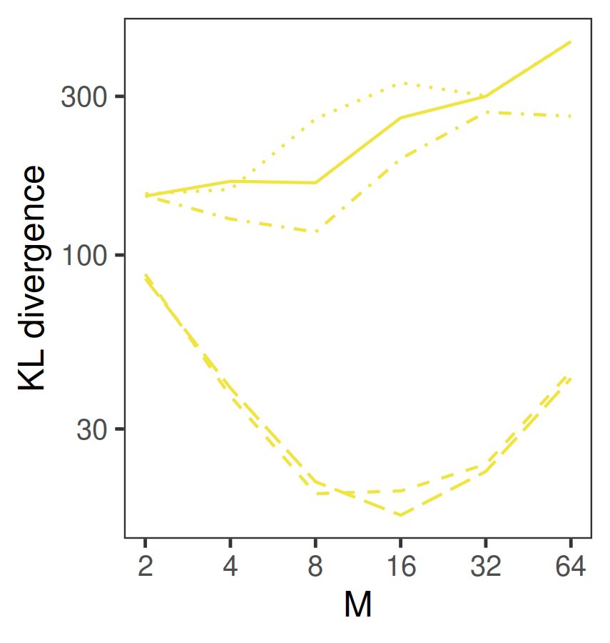
(k)

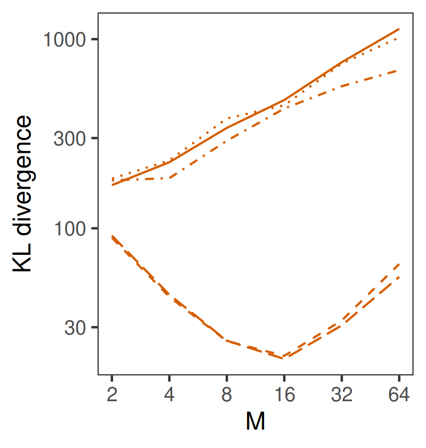
(l)

Figure 22: Posterior approximation comparisons for the $\Sigma$ marginal of the posterior in the MVN example of Section 3.2 with $\Sigma$ unknown and $d=8$ and $n=10,000$. The error in estimating (a)(d)(g) the posterior mean, (b)(e)(h) the 2.5% quantiles, (c)(f)(i) the 97.5% quantiles. (j)(k)(l) The KL divergence from the marginal of the posterior to each approximation.

D.1.1 Gamma GLM for diagnostics

All gamma GLMs with the log link, MVN studies with $d=8,n=10,000$.

KL divergence for $\mu$, all LEMIE models

Null deviance: 139.201 (86 dof), residual deviance: 68.056 (83 dof).

	Estimate	Std. Error	t value	Pr(>|t|)
(Intercept)	2.4118422	0.1294829	18.627	< 2e-16
ess	-0.0134534	0.0079883	-1.684	0.0959
khat	0.0316572	0.0034003	9.31	1.57E-14
ess:khat	-0.0002122	0.0001274	-1.666	0.0995

KL divergence for $\Sigma$, all LEMIE models

Null deviance: 91.982 (86 dof), residual deviance: 53.109 (83 dof).

	Estimate	Std. Error	t value	Pr(>|t|)
(Intercept)	4.65E+00	1.07E-01	43.253	< 2e-16
ess	-1.83E-02	6.63E-03	-2.762	0.00707
khat	2.07E-02	2.82E-03	7.347	1.27E-10
ess:khat	9.68E-05	1.06E-04	0.916	0.36242

KL divergence for $\mu$, LEMIE2 and LEMIE3 only

Null deviance: 105.701 (56 dof), residual deviance: 55.662 (53 dof).

	Estimate	Std. Error	t value	Pr(>|t|)
(Intercept)	2.745086	0.198363	13.839	< 2e-16
ess	-0.057005	0.038233	-1.491	0.142
khat	0.03612	0.007583	4.763	1.52E-05
ess:khat	-0.009408	0.006542	-1.438	0.156

KL divergence for $\Sigma$, LEMIE2 and LEMIE3 only

Null deviance: 63.574 (56 dof), residual deviance: 38.942 (53 dof).

	Estimate	Std. Error	t value	Pr(>|t|)
(Intercept)	4.769317	0.167882	28.409	<2e-16
ess	-0.029969	0.032358	-0.926	0.3586
khat	0.022828	0.006418	3.557	0.0008
ess:khat	-0.004623	0.005537	-0.835	0.4075

D.2 Logistic regression - simulation of Scott et al., (2016)

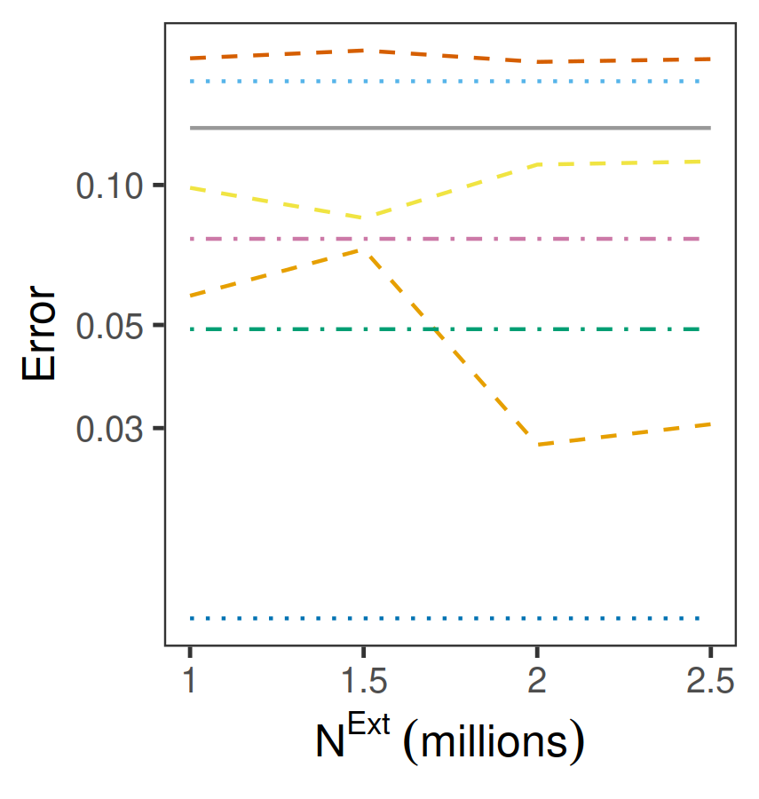
(a) Error in estimating the posterior mean of $\theta$.

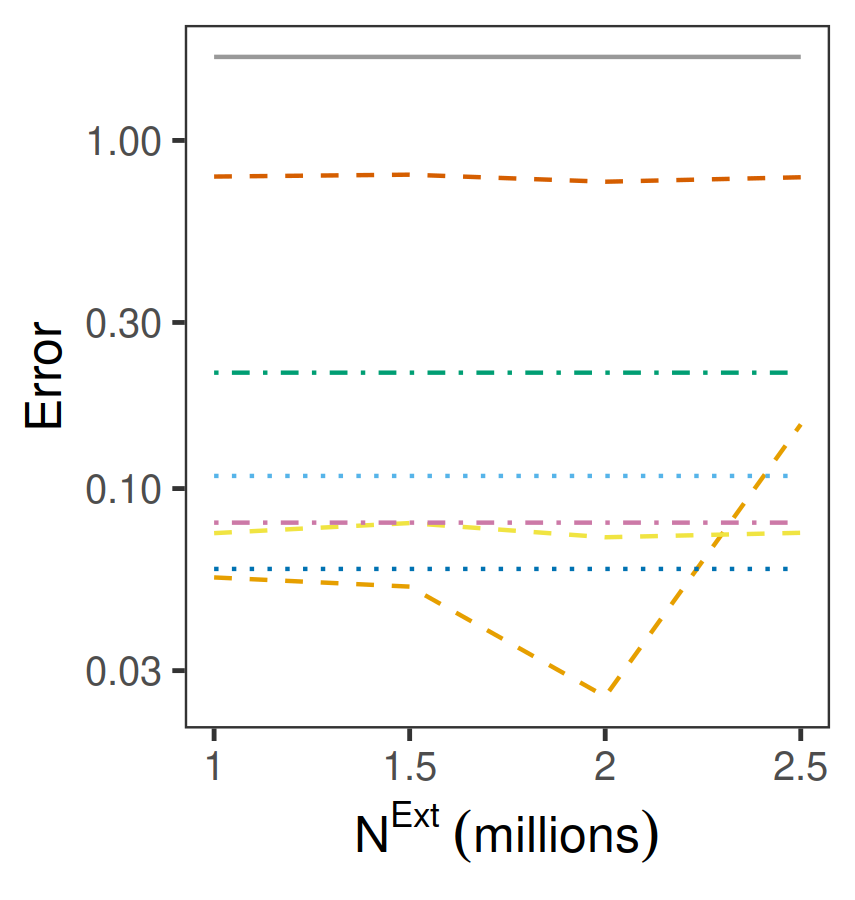
(b) Error in estimating the 2.5% quantiles of the marginals of the posterior.

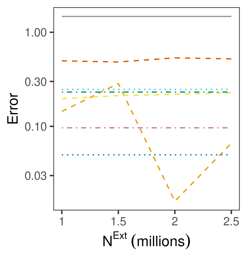
(c) Error in estimating the 97.5% quantiles of the marginals of the posterior.

Figure 24: Effect on performance metrics of adding more Laplace samples (of all types from Section 2.3) in the logistic example of Section 3.3.1. $N^{\textrm{{Ext}}}$ is the total number of Laplace samples added.

See Figure 24 for the results from Section 2.3, showing what happens to performance when we add more Laplace samples up to $2.5\times 10^{6}$.

References

- Amazon Web Services, Inc., (2017) Amazon Web Services, Inc. (2017). Elastic Compute Cloud (EC2) - Cloud Server & Hosting - AWS. [online] Available at: <https://aws.amazon.com/ec2/>.
- Apache Hadoop, (2018) Apache Hadoop (2018). Apache Hadoop project. [online] Available at: <http://hadoop.apache.org/>.
- Bardenet et al., (2017) Bardenet, R., Doucet, A., and Holmes, C. C. (2017). On markov chain monte carlo methods for tall data. Journal of Machine Learning Research, 18(47).
- Borthakur, (2007) Borthakur, D. (2007). The hadoop distributed file system: Architecture and design. Hadoop Project Website, 11(2007):21.
- Bryant et al., (2008) Bryant, R., Katz, R. H., and Lazowska, E. D. (2008). Big-data computing: creating revolutionary breakthroughs in commerce, science and society.
- Cover and Thomas, (2006) Cover, T. M. and Thomas, J. A. (2006). Elements of information theory, 2nd edition. Wiley.
- Dean and Ghemawat, (2008) Dean, J. and Ghemawat, S. (2008). Mapreduce: simplified data processing on large clusters. Communications of the ACM, 51(1):107–113.
- DerSimonian and Laird, (1986) DerSimonian, R. and Laird, N. (1986). Meta-analysis in clinical trials. Controlled clinical trials, 7(3):177–188.
- Dwork, (2008) Dwork, C. (2008). Differential privacy: A survey of results. In International conference on theory and applications of models of computation, pages 1–19. Springer.
- Elvira and Martino, (2021) Elvira, V. and Martino, L. (2021). Advances in importance sampling. arXiv preprint arXiv:2102.05407.
- Elvira et al., (2018) Elvira, V., Martino, L., and Robert, C. P. (2018). Rethinking the effective sample size. International Statistical Review.
- Gelman et al., (2004) Gelman, A., Carlin, J. B., Stern, H. S., and Rubin, D. B. (2004). Bayesian data analysis. Chapman and Hall/CRC.
- Gelman et al., (2008) Gelman, A., Jakulin, A., Pittau, M. G., and Su, Y.-S. (2008). A weakly informative default prior distribution for logistic and other regression models. The annals of applied statistics, 2(4):1360–1383.
- Green et al., (2015) Green, P. J., Łatuszyński, K., Pereyra, M., and Robert, C. P. (2015). Bayesian computation: a summary of the current state, and samples backwards and forwards. Statistics and Computing, 25(4):835–862.
- Herlihy et al., (2020) Herlihy, M., Shavit, N., Luchangco, V., and Spear, M. (2020). The art of multiprocessor programming. Newnes.
- Hesterberg, (1995) Hesterberg, T. (1995). Weighted average importance sampling and defensive mixture distributions. Technometrics, 37(2):185–194.
- Huang and Gelman, (2005) Huang, Z. and Gelman, A. (2005). Sampling for bayesian computation with large datasets. Available at SSRN 1010107.
- Jordan et al., (2018) Jordan, M. I., Lee, J. D., and Yang, Y. (2018). Communication-efficient distributed statistical inference. Journal of the American Statistical Association.
- Kalavri and Vlassov, (2013) Kalavri, V. and Vlassov, V. (2013). Mapreduce: Limitations, optimizations and open issues. In 2013 12th IEEE international conference on trust, security and privacy in computing and communications, pages 1031–1038. IEEE.
- Kong, (1992) Kong, A. (1992). A note on importance sampling using standardized weights. University of Chicago, Dept. of Statistics, Tech. Rep, 348.
- Lao et al., (2020) Lao, J., Suter, C., Langmore, I., Chimisov, C., Saxena, A., Sountsov, P., Moore, D., Saurous, R. A., Hoffman, M. D., and Dillon, J. V. (2020). tfp. mcmc: Modern markov chain monte carlo tools built for modern hardware. arXiv preprint arXiv:2002.01184.
- Lee et al., (2010) Lee, A., Yau, C., Giles, M. B., Doucet, A., and Holmes, C. C. (2010). On the utility of graphics cards to perform massively parallel simulation of advanced monte carlo methods. Journal of computational and graphical statistics, 19(4):769–789.
- Liu and Liu, (2001) Liu, J. S. and Liu, J. S. (2001). Monte Carlo strategies in scientific computing, volume 10. Springer.
- Luengo et al., (2015) Luengo, D., Martino, L., Elvira, V., and Bugallo, M. (2015). Bias correction for distributed bayesian estimators. In 2015 IEEE 6th International Workshop on Computational Advances in Multi-Sensor Adaptive Processing (CAMSAP), pages 253–256. IEEE.
- Luengo et al., (2018) Luengo, D., Martino, L., Elvira, V., and Bugallo, M. (2018). Efficient linear fusion of partial estimators. Digital Signal Processing, 78:265–283.
- Ma et al., (2021) Ma, T., Hoang, T. N., and Chen, J. (2021). Federated inference through aligning local representations and learning a consensus graph. ICLR 2022 Submitted.
- MacKay et al., (2003) MacKay, D. J., Mac Kay, D. J., et al. (2003). Information theory, inference and learning algorithms. Cambridge university press.
- Medina-Aguayo and Everitt, (2019) Medina-Aguayo, F. J. and Everitt, R. G. (2019). Revisiting the balance heuristic for estimating normalising constants. arXiv preprint arXiv:1908.06514.
- Neiswanger et al., (2013) Neiswanger, W., Wang, C., and Xing, E. (2013). Asymptotically exact, embarrassingly parallel mcmc. arXiv preprint arXiv:1311.4780.
- Neiswanger et al., (2015) Neiswanger, W., Wang, C., and Xing, E. (2015). Embarrassingly parallel variational inference in nonconjugate models. arXiv preprint arXiv:1510.04163.
- Nemeth and Sherlock, (2018) Nemeth, C. and Sherlock, C. (2018). Merging mcmc subposteriors through gaussian-process approximations. Bayesian Analysis, 13(2):507–530.
- Newman et al., (2009) Newman, D., Asuncion, A., Smyth, P., and Welling, M. (2009). Distributed algorithms for topic models. Journal of Machine Learning Research, 10(8).
- Owen, (2013) Owen, A. B. (2013). Monte Carlo theory, methods and examples. Stanford.
- Park et al., (2020) Park, M., Foulds, J., Chaudhuri, K., and Welling, M. (2020). Variational bayes in private settings (vips). Journal of Artificial Intelligence Research, 68:109–157.
- Pickands III, (1975) Pickands III, J. (1975). Statistical inference using extreme order statistics. the Annals of Statistics, pages 119–131.
- Polson et al., (2013) Polson, N. G., Scott, J. G., and Windle, J. (2013). Bayesian inference for logistic models using pólya–gamma latent variables. Journal of the American statistical Association, 108(504):1339–1349.
- R Core Team, (2020) R Core Team (2020). R: A Language and Environment for Statistical Computing. R Foundation for Statistical Computing, Vienna, Austria <https://www.R-project.org/>.
- Rendell et al., (2020) Rendell, L. J., Johansen, A. M., Lee, A., and Whiteley, N. (2020). Global consensus monte carlo. Journal of Computational and Graphical Statistics, 30(2):249–259.
- Robert and Casella, (2004) Robert, C. P. and Casella, G. (2004). Monte Carlo statistical methods. Springer, second edition.
- Sagiroglu and Sinanc, (2013) Sagiroglu, S. and Sinanc, D. (2013). Big data: A review. In 2013 international conference on collaboration technologies and systems (CTS), pages 42–47. IEEE.
- Sarkar et al., (2015) Sarkar, A., Ghosh, A., and Nath, D. A. (2015). Mapreduce: A comprehensive study on applications, scope and challenges. Department of Computer Science, International Journal of Advance Research in Computer Science and Management Studies, 3(7).
- Scott et al., (2016) Scott, S. L., Blocker, A. W., Bonassi, F. V., Chipman, H. A., George, E. I., and McCulloch, R. E. (2016). Bayes and big data: The consensus monte carlo algorithm. International Journal of Management Science and Engineering Management, 11(2):78–88.
- Stan Development Team, (2022) Stan Development Team (2022). Stan Modeling Language Users Guide and Reference Manual. Version 2.30, [online] Available at: https://mc-stan.org/>.
- Torra and Navarro-Arribas, (2016) Torra, V. and Navarro-Arribas, G. (2016). Big data privacy and anonymization. In IFIP International Summer School on Privacy and Identity Management, pages 15–26. Springer.
- Van der Vaart, (1998) Van der Vaart, A. W. (1998). Asymptotic statistics. Cambridge university press.
- Vats et al., (2019) Vats, D., Flegal, J. M., and Jones, G. L. (2019). Multivariate output analysis for markov chain monte carlo. Biometrika, 106(2):321–337.
- Veach and Guibas, (1995) Veach, E. and Guibas, L. J. (1995). Optimally combining sampling techniques for monte carlo rendering. In Proceedings of the 22nd annual conference on Computer graphics and interactive techniques, pages 419–428.
- Vehtari et al., (2022) Vehtari, A., Gabry, J., Magnusson, M., Yao, Y., Bürkner, P., Paananen, T., and Gelman, A. (2022). loo: Efficient leave-one-out cross-validation and WAIC for Bayesian models. R package version 2.5.1, <URL:https://mc-stan.org/loo/>.
- Vehtari et al., (2017) Vehtari, A., Gelman, A., and Gabry, J. (2017). Practical bayesian model evaluation using leave-one-out cross-validation and waic. Statistics and computing, 27(5):1413–1432.
- Vehtari et al., (2015) Vehtari, A., Simpson, D., Gelman, A., Yao, Y., and Gabry, J. (2015). Pareto smoothed importance sampling. arXiv preprint arXiv:1507.02646.
- Vono et al., (2018) Vono, M., Dobigeon, N., and Chainais, P. (2018). Sparse bayesian binary logistic regression using the split-and-augmented gibbs sampler. In 2018 IEEE 28th International Workshop on Machine Learning for Signal Processing (MLSP), pages 1–6. IEEE.
- Vono et al., (2019) Vono, M., Paulin, D., and Doucet, A. (2019). Efficient mcmc sampling with dimension-free convergence rate using admm-type splitting. arXiv preprint arXiv:1905.11937.
- Wang and Dunson, (2013) Wang, X. and Dunson, D. B. (2013). Parallelizing mcmc via weierstrass sampler. arXiv preprint arXiv:1312.4605.
- Xiong et al., (2021) Xiong, R., Koenecke, A., Powell, M., Shen, Z., Vogelstein, J. T., and Athey, S. (2021). Federated causal inference in heterogeneous observational data. arXiv preprint arXiv:2107.11732.
- Xu et al., (2014) Xu, M., Lakshminarayanan, B., Teh, Y. W., Zhu, J., and Zhang, B. (2014). Distributed bayesian posterior sampling via moment sharing. Advances in Neural Information Processing Systems, 27.
- Zaharia et al., (2010) Zaharia, M., Chowdhury, M., Franklin, M. J., Shenker, S., and Stoica, I. (2010). Spark: Cluster computing with working sets. In 2nd USENIX Workshop on Hot Topics in Cloud Computing (HotCloud 10).
- Zhang and Stephens, (2009) Zhang, J. and Stephens, M. A. (2009). A new and efficient estimation method for the generalized pareto distribution. Technometrics, 51(3):316–325.