Genus $g$ Cantor sets and Germane Julia sets

Abstract.

The main aim of this paper is to give topological obstructions to Cantor sets in $\mathbb{R}^{3}$ being Julia sets of uniformly quasiregular mappings. Our main tool is the genus of a Cantor set. We give a new construction of a genus $g$ Cantor set, the first for which the local genus is $g$ at every point, and then show that this Cantor set can be realized as the Julia set of a uniformly quasiregular mapping. These are the first such Cantor Julia sets constructed for $g\geq 3$. We then turn to our dynamical applications and show that every Cantor Julia set of a hyperbolic uniformly quasiregular map has a finite genus $g$; that a given local genus in a Cantor Julia set must occur on a dense subset of the Julia set; and that there do exist Cantor Julia sets where the local genus is non-constant.

1. Introduction

It is well-known that the Julia set $J(f)$ of a rational map $f$ can be a Cantor set. The simplest examples arise for quadratic polynomials $z^{2}+c$ when $c$ is not in the Mandelbrot set. It is also well known that every Cantor set embedded in $\overline{\mathbb{R}^{2}}$ has a defining sequence consisting of topological disks, that is, every such Cantor set arises as an infinite intersection of a collection of nested disks, see [Moi77].

The goal of the current paper is to study topological properties of Julia sets of uniformly quasiregular mappings (henceforth denoted by UQR mappings) in $\overline{\mathbb{R}^{3}}$ and, in particular, when they are Cantor sets, what sort of defining sequences they can have. UQR mappings provide the setting for the closest counterpart to complex dynamics in $\mathbb{S}^{3}$ and, more generally, higher real dimensions. We will, however, stay in dimension three in this paper as this provides the setting to consider the genus of a Cantor set as introduced by Željko [Ž05] based on the notion of defining sequences from Armentrout [Arm66].

The first examples of uniformly quasiregular mappings constructed by Iwaniec and Martin [IM96] have a Cantor set as the Julia set. Moreover, although this was not of concern to the authors, from their construction it is evident that the Julia set is a tame Cantor set. This means that the Cantor set can be mapped via an ambient homeomorphism of $\overline{\mathbb{R}}^{3}$ onto the standard ternary Cantor set contained in a line. Equivalently, this means the Cantor set has a defining sequence consisting of topological $3$-balls. Moreover, such a Cantor set $X$ is then said to have genus zero, written $g(X)=0$.

If a Cantor set is not tame, then it is called wild. The standard example of a wild Cantor set in $\mathbb{R}^{3}$ is Antoine’s necklace. The first named author and Wu [FW15] constructed a UQR map for which the Julia set is an Antoine’s necklace that has genus $1$. More recently, the first and second named authors [FS21] showed via a more intricate construction that there exist uniformly quasiregular mappings whose Julia sets are genus $2$ Cantor sets.

The first main aim of the current paper is to give a general construction which will apply to all genera. This will necessitate a new topological construction since, as far as the authors are aware, the only construction of genus $g$ Cantor sets for all $g$ are given by Željko [Ž05] and this construction cannot yield Julia sets. The local genus $g_{x}(X)$ of a Cantor set $X$ at $x\in X$ describes the genus of handlebodies required in a defining sequence in any neighborhood of $x$. Željko’s construction has local genus one except at one point. Our first main result reads as follows.

Theorem 1.1.

For each $g\in\mathbb{N}$ there exists a UQR map $f_{g}:\overline{\mathbb{R}^{3}}\to\overline{\mathbb{R}^{3}}$ for which the Julia set $J(f_{g})$ is a Cantor set of genus $g$ and, moreover, for each $x\in J(f_{g})$, the local genus $g_{x}(J(f_{g}))=g$.

We remark that the genus $1$ case of Theorem 1.1 recovers Antoine’s necklace, whereas the genus $2$ case is substantially different from the construction in [FS21]. For all higher genera, Theorem 1.1 provides a new construction. This construction is necessarily highly intricate as it needs to be amenable to our dynamical applications.

Next, we turn to topological obstructions for Cantor sets in $\overline{\mathbb{R}^{3}}$ being Julia sets based on the genus. It is an important theme in dynamics to give geometric or topological restrictions on the Julia set, once a toplogical type has been fixed. The first named author and Nicks [FN11] showed that the Julia set of a UQR mapping in $\overline{\mathbb{R}^{n}}$ is uniformly perfect, that is, ring domains which separate points of the Julia set cannot be too thick. As a counterpart to this result, it was shown by the first and third named authors [FV21], that if the Julia set of a hyperbolic UQR mapping in $\overline{\mathbb{R}^{n}}$ is totally disconnected, then it is uniformly disconnected. Here, a uniformly quasiregular mapping is hyperbolic if the Julia set does not meet the closure of the post-branch set. Roughly speaking, this result says that ring domains separating points of the Julia set cannot be forced to be too thin.

The above results place geometric conditions on which Cantor sets can be Julia sets. Our second main result places a topological restriction on which Cantor sets can be Julia sets.

Theorem 1.2.

Let $f:\overline{\mathbb{R}^{3}}\to\overline{\mathbb{R}^{3}}$ be a hyperbolic uqr map for which $J(f)$ is a Cantor set. Then there exists $g\in\mathbb{N}\cup\{0\}$ such that the genus of $J(f)$ is $g$.

There do exist Cantor sets of infinite genus, see [Ž05, Theorem 5], and so Theorem 1.2 rules these out as possibilities for Julia sets. We recall that the backwards orbit of $x$ is

$$O^{-}(x)=\{y:f^{m}(y)=x\text{ for some }m\in\mathbb{N}\},$$

and the grand orbit is

$$GO(x)=\{y:f^{m_{1}}(y)=f^{m_{2}}(x)\text{ for some }m_{1},m_{2}\in\mathbb{N}\}.$$

Our next result is on the local genus of points in the Julia set.

Theorem 1.3.

Let $f:\overline{\mathbb{R}^{3}}\to\overline{\mathbb{R}^{3}}$ be a hyperbolic uqr map for which $J(f)$ is a Cantor set. If the local genus $g_{x}(J(f))=g\in\mathbb{N}\cup\{0\}$, then $g_{y}(J(f))=g$ for every $y$ in the grand orbit $GO(x)$ of $x$.

As the backwards orbit of a point in $J(f)$ is dense in $J(f)$, we immediately have the following corollary.

Corollary 1.4.

Let $f:\overline{\mathbb{R}^{3}}\to\overline{\mathbb{R}^{3}}$ be a hyperbolic uqr map with $J(f)$ a Cantor set. Suppose there exists $x\in J(f)$ with $g_{x}(J(f))=g$. Then the set of points in $J(f)$ for which the local genus is $g$ is dense in $J(f)$.

This result places further severe restrictions on which Cantor sets can be Julia sets. The constructions in [Ž05, Theorem 5] which yield Cantor sets of genus $g\in\mathbb{N}$ have the property that there is a special point $x\in X$ for which $g_{x}(X)=g$ and $g_{y}(X)=1$ for all other points $y\in X\setminus\{x\}$. Corollary 1.4 then implies that these Cantor sets cannot be Julia sets.

Since the examples of Julia sets in [FS21, FW15] have constant local genus, it is natural to ask if this is always the case for Julia sets which are Cantor sets. Our final result shows that this is not the case.

Theorem 1.5.

Let $g\geq 1$. There exists a UQR map $f:\overline{\mathbb{R}^{3}}\to\overline{\mathbb{R}^{3}}$ such that $J(f)$ is a Cantor set of genus $g$, and there exist points with local genus $g$ and other points with local genus $0$.

It would be interesting to know whether any finite collection of non-negative integers can be realized as the local genera of a Cantor Julia set.

The paper is organized as follows. In Section 2 we recall some preliminary material on UQR maps and the genus of Cantor sets. In Section 3 we construct a Cantor set $X_{g}$ for each $g\geq 1$. In Section 4, we prove that $X_{g}$ has genus $g$ and local genus $g$ at each point. In Section 5 we complete the proof of Theorem 1.1 by constructing a UQR map with Julia set equal to $X_{g}$. In Section 6 we prove Theorem 1.2 and Theorem 1.3. Finally, in Section 7 we construct an example that proves Theorem 1.5.

2. Preliminaries

We denote by $\overline{\mathbb{R}^{n}}$ the one point compactification of $\mathbb{R}^{n}$.

2.1. Uniformly quasiregular mappings

A continuous map $f:\mathbb{R}^{n}\to\mathbb{R}^{n}$ is called quasiregular if $f$ belongs to the Sobolev space $W^{1,n}_{\text{loc}}(\mathbb{R}^{n})$ and if there exists some $K\geq 1$ such that

(2.1) $$|f^{\prime}(x)|^{n}\leq KJ_{f}(x)\qquad\text{for a.e. $x\in\mathbb{R}^{n}$}.$$

Here $J_{f}$ denotes the Jacobian of $f$ at $x\in\mathbb{R}^{n}$ and $|f^{\prime}(x)|$ the operator norm. If $f$ is quasiregular, then there exists $K^{\prime}\geq 1$ such that

(2.2) $$J_{f}(x)\leq K^{\prime}\min_{|h|=1}|f^{\prime}(x)(h)|\qquad\text{ for a.e. $x\in\mathbb{R}^{n}$}.$$

The maximal dilatation $K(f)$ of a quasiregular map $f$ is the smallest $K$ that satisfies both equations (2.1) and (2.2). The maximal dilatation $K(f)$ can be informally thought of as a quantity describing how much distortion $f$ has. The closer $K(f)\in[1,\infty)$ is to $1$, the closer $f$ is to a conformal map. If $K(f)\leq K$, then we say that $f$ is $K$-quasiregular. See Rickman’s monograph [Ric93] for a complete exposition on quasiregular mappings.

Quasiregular mappings can be defined at infinity and also take on the value infinity. To do this, if $A:\mathbb{S}^{n}\to\mathbb{S}^{n}$ is a Möbius map with $A(\infty)=0$, then we require $f\circ A^{-1}$ or $A\circ f$ respectively to be quasiregular via the definition above.

The composition $f\circ g$ of two quasiregular mappings $f$ and $g$ is again quasiregular, but typically the maximal dilatation goes up. We say that $f:\overline{\mathbb{R}^{n}}\to\overline{\mathbb{R}^{n}}$ is uniformly quasiregular, abbreviated to UQR, if the maximal dilatations of all the iterates of $f$ are uniformly bounded above.

For a UQR map, the definitions of the Julia set and Fatou set are identical to those in complex dynamics: the Fatou set $F(f)$ is the domain of local normality of the family of the iterates and the Julia set $J(f)$ is the complement.

The branch set $\mathcal{B}(f)$ of a UQR map $f:\overline{\mathbb{R}^{n}}\to\overline{\mathbb{R}^{n}}$ is the closed set of points in $\overline{\mathbb{R}^{n}}$ where $f$ does not define a local homeomorphism. The post-branch set of non-injective UQR map $f$ is

$$\mathcal{P}(f)=\overline{\{f^{m}(\mathcal{B}(f)):m\geq 0\}}.$$

The map $f$ is called hyperbolic if $J(f)\cap\mathcal{P}(f)$ is empty.

We will need the following result regarding injective restrictions of hyperbolic uqr maps near the Julia set.

Lemma 2.1 ([FV21], Lemma 3.3 and the proof of Theorem 3.4).

Suppose that $n\geq 2$ and $f:\mathbb{S}^{n}\to\mathbb{S}^{n}$ is a hyperbolic UQR map. There exists $r_{1}>0$ such that if $x\in J(f)$, then $f$ is injective on $B(x,r_{1})$. Moreover, there exists $N\in\mathbb{N}$ such that if $U$ is an $r_{1}$-neighbourhood of $J(f)$, then $\overline{f^{-N}(U)}\subset U$.

2.2. Cantor sets and genus

Recall that a Cantor set is any metric space homeomorphic to the usual Cantor ternary set. Two Cantor sets $E_{1},E_{2}\subset\overline{\mathbb{R}^{n}}$ are equivalently embedded (or ambiently homeomorphic) if there exists a homeomorphism $\psi:\overline{\mathbb{R}^{n}}\to\overline{\mathbb{R}^{n}}$ such that $\psi(E_{1})=E_{2}$. If the Cantor set $E$ is equivalently embedded to the usual Cantor ternary set in a line, then $E$ is called tame. A Cantor set which is not tame is called wild. We often assume that $\infty\notin E$ so we may consider $E\subset\mathbb{R}^{n}$.

Other examples of Cantor sets in $\overline{\mathbb{R}^{n}}$ are typically defined in terms of a similar construction to above, using an intersection of nested unions of compact $n$-manifolds with boundary. For Cantor sets in $\mathbb{R}^{3}$, the idea of defining sequences goes back to Armentrout [Arm66]. This can be easily generalized to Cantor sets in $\overline{\mathbb{R}^{3}}$ by applying a Möbius map so as to move the Cantor set to $\mathbb{R}^{3}$.

Definition 2.2.

A defining sequence for a Cantor set $E\subset\mathbb{R}^{3}$ is a sequence $(M_{i})$ of compact 3-manifolds with boundary such that

1. each $M_{i}$ consists of disjoint polyhedral cubes with handles,

2. $M_{i+1}\subset M_{i}$ for each $i$, and

3. $E=\bigcap_{i}M_{i}$.

We denote the set of all defining sequences for $E$ by $\mathcal{D}(E)$.

If $M$ is a topological cube with handles, denote the number of handles of $M$ by $g(M)$. For a disjoint union of cubes with handles $M=\sqcup_{i\in I}M_{i}$, we set $g(M)=\sup\{g(M_{i}):i\in I\}$. The genus of a Cantor set was introduced by Željko, see [Ž05, p. 350].

Definition 2.3.

Let $(M_{i})$ be a defining sequence for the Cantor set $E\subset\mathbb{R}^{3}$. Define

$$g(E;(M_{i}))=\sup\{g(M_{i}):i\geq 0\}.$$

Then define the genus of the Cantor set $E$ as

$$g(E)=\inf\{g(E;(M_{i})):(M_{i})\in\mathcal{D}(E)\}.$$

Now let $x\in E$. Denote by $M_{i}^{x}$ the union of all the components of $M_{i}$ containing $x$. Similar to above, define

$$g_{x}(E;(M_{i}))=\sup\{g(M_{i}^{x}):i\geq 0\}.$$

Then define the local genus of $E$ at the point $x$ as

$$g_{x}(E)=\inf\{g_{x}(E;(M_{i})):(M_{i})\in\mathcal{D}(E)\}.$$

3. Construction of a genus $g$ self-similar Cantor set

3.1. Some sequences

We start by defining a “folding” sequence that will help us keep track of various folding maps that will be required later on. For each $n\in\mathbb{N}$ and each $k\in\{1,\dots,n\}$ define $a_{n,k}\in\mathbb{N}$ with $a_{1,1}=1$ and for $m\in\mathbb{N}$

$$a_{2m,k} =\begin{cases}a_{m,k}&\text{if $1\leq k\leq m$}\\ a_{m,2m-k+1}&\text{if $m+1\leq k\leq 2m$},\end{cases}$$

$$a_{2m+1,k} =\begin{cases}a_{m+1,k}&\text{if $1\leq k\leq m$}\\ 2a_{m+1,m+1}&\text{if $k=m+1$}\\ a_{m+1,2m-k+2}&\text{if $m+2\leq k\leq 2m+1$}.\end{cases}$$

Lemma 3.1.

For all $n\in\mathbb{N}$ and $k\in\{1,\dots,n\}$ we have $a_{n,k}\in\{1,2\}$.

Proof.

We prove the following claim: for all $n\in\mathbb{N}$

1. $\{a_{n,k}:1\leq k\leq n\}\subset\{1,2\}$

2. $a_{n,n}=a_{n,1}=1$.

The proof of the claim is by induction on $n$. The claim is clear for $n=1$. Assume now the claim to be true for all integers $n<N$ for some $N\in\mathbb{N}$.

If $N=2m$, then

$$\{a_{2m,k}:1\leq k\leq 2m\}=\{a_{m,k}:1\leq k\leq m\}\subset\{1,2\}$$

while $a_{2m,1}=a_{m,1}=1$ and $a_{2m,2m}=a_{m,1}=1$.

If $N=2m+1$, then

$$\{a_{2m+1,k}:1\leq k\leq 2m,k\neq m+1\}=\{a_{m+1,k}:1\leq k\leq m\}\subset\{1,2\}$$

and $a_{2m+1,m+1}=2a_{m+1,m+1}=2$. Moreover,

$$a_{2m+1,1}=a_{m+1,1}=1\quad\text{and}\quad a_{2m+1,2m+1}=a_{m+1,1}=1.\qed$$

For each $n\in\mathbb{N}$ we define a finite sequence $(c_{n,i})_{i=1}^{n}$ by

$$c_{n,i}=\begin{cases}1&\text{ if $a_{n,i}=1$}\\ 3&\text{ if $a_{n,i}=2$}.\end{cases}$$

Set $C_{n,0}=0$ and for each $i\in\{1,\dots,n\}$, set

$$C_{n,i}=c_{n,1}+\cdots+c_{n,i}.$$

For each $g\in\mathbb{N}$ we fix for the rest of the paper an odd square integer $N_{g}\in\mathbb{N}$ such that

(3.1) $$N_{g}\geq 48\sqrt{2}(C_{g,g}+6).$$

This important integer is related to the number of handelbodies required at each stage of the defining sequence of the Cantor set to be constructed.

3.2. A $g$-ladder

Fix $g\in\mathbb{N}$. To ease the notation, for the rest of Section 3, we write $N_{g}=N$, $c_{g,i}=c_{i}$ and $C_{g,i}=C_{i}$.

For each $i\in\{1,\dots,g\}$ define the planar simple closed curve

(3.2) $$\gamma_{i}=\partial\left([C_{i-1},C_{i}]\times[0,1]\right).$$

Note that each ${\gamma}_{i}$ is either a translated copy of $\partial[0,1]^{2}$ or a translated copy of $\partial([0,3]\times[0,1])$. Define also the planar closed curve

$$\gamma=\gamma_{1}\cup\cdots\cup\gamma_{g}.$$

See Figure 1 for $\gamma$ in the case that $g=6$.

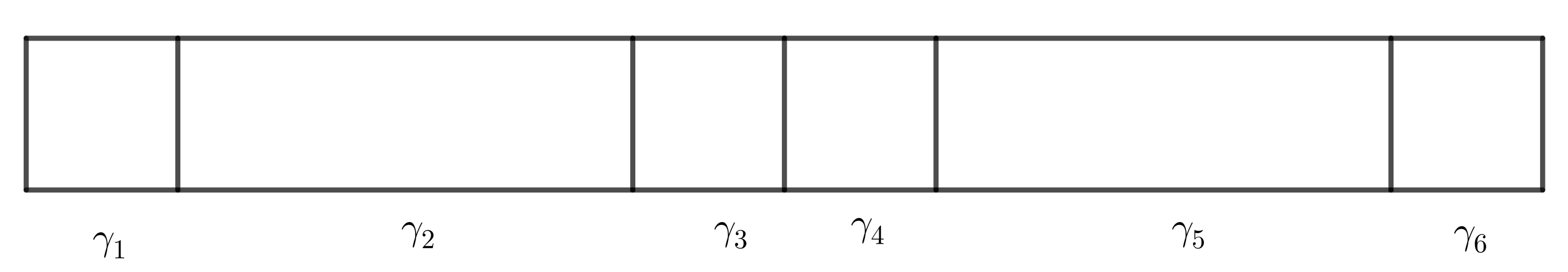
Figure 1. The curve $\gamma$ in the case that $g=6$. In this case, $(a_{6,i})=(1,2,1,1,2,1)$.

3.3. A chain of $g$-ladders

For each $i\in\{1,\dots,g\}$ we define rescaled copies $\tau_{i,j}$ of $\gamma$. Fix $i\in\{1,\dots,g\}$. Let $x_{i,1}=(C_{i-1}+\frac{1}{2N},1)$, $x_{i,c_{i}N}=(C_{i}-\frac{1}{2N},1)$, $x_{i,(c_{i}+1)N+1}=(C_{i}-\frac{1}{2N},0)$, $x_{i,(2c_{i}+1)N+1}=(C_{i-1}+\frac{1}{2N},0)$, and define also

$$x_{i,j}=\begin{cases}(a+j/N,1),&\text{ if $j=2,\dots,c_{i}N$}\\ (a+1,1-(j-c_{i}N-1)/N),&\text{ if $j=c_{i}N+2,\dots,(c_{i}+1)N$}\\ (a+1-(j-(c_{i}+1)N-1)/N,0),&\text{ if $j=c_{i}(N+1)+2,\dots,(2c_{i}+1)N$}\\ (a,(j-(2c_{i}+1)N-1)/N),&\text{ if $j=(2c_{i}+1)N+2,\dots,(2c_{i}+2)N$}.\\ \end{cases}$$

Therefore, the points $\{x_{i,1},\dots,x_{i,2(c_{i}+1)N}\}$ lie on ${\gamma}_{i}$ oriented clockwise.

For each $j\in\{1,\dots,2(c_{i}+1)N\}$, let $\sigma_{i,j}$ be a line segment in $\mathbb{R}^{2}$ centered at $x_{i,j}$, of length $8\sqrt{2}(5N)^{-1}$, such that

1. $\sigma_{i,j}$ is vertical to $\gamma_{i}$ if $j\in\{1,c_{i}N+1,(c_{i}+1)N+1,(2c_{i}+1)N\}$;

2. $\sigma_{i,j}$ has slope $-1$ if

   1. $j\in\{2,4,\dots,c_{i}N-1\}$,

   2. or if $j\in\{c_{i}N+2,c_{i}N+4,\dots,(c_{i}+1)N-1\}$,

   3. or if $j\in\{(c_{i}+1)N+2,(c_{i}+1)N+4,\dots,(2c_{i}+1)N-1\}$,

   4. or if $j\in\{(2c_{i}+1)N+2,(2c_{i}+1)N+4,\dots,(2c_{i}+2)N-1\}$;

3. $\sigma_{i,j}$ has slope $1$ if

   1. $j\in\{3,5,\dots,c_{i}N\}$,

   2. or if $j\in\{c_{i}N+3,c_{i}N+5,\dots,(c_{i}+1)N\}$,

   3. or if $j\in\{(c_{i}+1)N+3,(c_{i}+1)N+5,\dots,(2c_{i}+1)N\}$,

   4. or if $j\in\{(2c_{i}+1)N+3,(2c_{i}+1)N+5,\dots,(2c_{i}+2)N\}$.

See Figure 2 for the case $c_{i}=1$ (for simplicity we have set $N=9$).

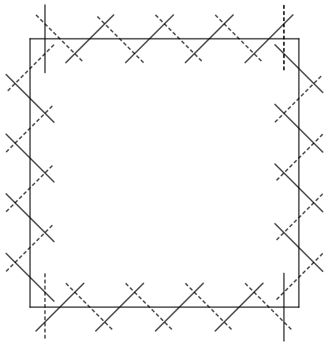
Figure 2. The segments $\sigma_{i,j}$ in the case that $c_{i}=1$ and $N=9$. The segments $\sigma_{i,j}$ with $j$ even, are depicted as dotted segments.

Lemma 3.2.

If $i,i^{\prime}\in\{1,\dots,g\}$, $j\in\{1,\dots,2(c_{i}+1)N\}$, and $j^{\prime}\in\{1,\dots,2(c_{i^{\prime}}+1)N\}$, then $\sigma_{i,j}\cap\sigma_{i^{\prime},j^{\prime}}\neq\emptyset$ if and only if one of the following is true:

1. $i=i^{\prime}$ and $|j-j^{\prime}|\in\{0,1\}$ modulo $(2c_{i}+2)N$ (that is, either $j=j^{\prime}$, or $x_{i,j}$, $x_{i,j^{\prime}}$ are consecutive on ${\gamma}^{i}_{0}$);

2. $|i-i^{\prime}|=1$ and $|x_{i,j}-x_{i^{\prime},j^{\prime}}|=0$.

Moreover, if $\sigma_{i,j}\cap\sigma_{i^{\prime},j^{\prime}}=\emptyset$, then $\operatorname{dist}(\sigma_{i,j},\sigma_{i^{\prime},j^{\prime}})\geq\sqrt{2}(5N)^{-1}$.

Proof.

To prove the lemma, we consider three possible cases.

Case 1: $i=i^{\prime}$. If $j=j^{\prime}$, then clearly $x_{i,j}=x_{i^{\prime},j^{\prime}}$ and $\sigma_{i,j}\cap\sigma_{i^{\prime},j^{\prime}}\neq\emptyset$. We assume for the rest of Case 1 that $j\neq j^{\prime}$ and consider four subcases.

Case 1.1: $|j-j^{\prime}|=1$ modulo $(2c_{i}+2)N$. It is easy to see by the design of the segments $\sigma_{i,j}$ that $\sigma_{i,j}\cap\sigma_{i^{\prime},j^{\prime}}\neq\emptyset$.

Case 1.2: $|j-j^{\prime}|=2$ modulo $(2c_{i}+2)N$ and $x_{i,j},x_{i,j^{\prime}}$ are both on the left edge or both are in the right edge. Then $\sigma_{i,j}$ and $\sigma_{i,j^{\prime}}$ are parallel and $\operatorname{dist}(\sigma_{i,j},\sigma_{i,j^{\prime}})=\sqrt{2}/N>\sqrt{2}(5N)^{-1}$.

Case 1.3: $|j-j^{\prime}|=2$ modulo $(2c_{i}+2)N$ and $x_{i,j},x_{i,j^{\prime}}$ are both on the top edge or both are on the bottom edge. Without loss of generality, assume that $x_{i,j},x_{i,j^{\prime}}$ are both on the top edge. Suppose first that $j,j^{\prime}\not\in\{1,c_{i}N+1\}$. Then, $\sigma_{i,j}$ and $\sigma_{i,j^{\prime}}$ are parallel and $\operatorname{dist}(\sigma_{i,j},\sigma_{i,j^{\prime}})=\sqrt{2}/N>\sqrt{2}(5N)^{-1}$. Suppose now that $j=1$; the other case is similar. Then, elementary calculations show that

$$\operatorname{dist}(\sigma_{i,j},\sigma_{i,j^{\prime}})=\tfrac{7}{16}8\sqrt{2}(5N)^{-1}>\sqrt{2}(5N)^{-1}.$$

Case 1.4: $|j-j^{\prime}|=2$ modulo $(2c_{i}+2)N$ and $x_{i,j},x_{i,j^{\prime}}$ are not on the same edge. Without loss of generality assume that $x_{i,j}$ is on the left edge and $x_{i,j^{\prime}}$ is on the top edge. If $j=2(c_{i}+1)N$ and $j^{\prime}=2$, then elementary calculations show that

$$\operatorname{dist}(\sigma_{i,j},\sigma_{i,j^{\prime}})=\tfrac{1}{8}8\sqrt{2}(5N)^{-1}=\sqrt{2}(5N)^{-1}.$$

If $j=2(c_{i}+1)N-1$ and $j=1$, then elementary calculations show that

$$\operatorname{dist}(\sigma_{i,j},\sigma_{i,j^{\prime}})=\tfrac{7}{16}8\sqrt{2}(5N)^{-1}>\sqrt{2}(5N)^{-1}.$$

Case 1.5: $|x_{i,j}-x_{i,j^{\prime}}|\not\in\{0,1,2\}$ modulo $(2c_{i}+2)N$. Note that $|x_{i,j}-x_{i,j^{\prime}}|\geq\sqrt{5}/N$. Suppose first that $|x_{i,j}-x_{i,j^{\prime}}|=\sqrt{5}/N$. This is the case where one of the two points $x_{i,j},x_{i,j^{\prime}}$ (say $x_{i,j}$) is either on the left or on the right edge, and the other point $x_{i,j^{\prime}}$ is either on the top or on the bottom edge. In either case, $\sigma_{i,j}$ is parallel to $\sigma_{i,j^{\prime}}$ and elementary calculations give

$$\operatorname{dist}(\sigma_{i,j},\sigma_{i,j^{\prime}})\geq(\sqrt{2}N)^{-1}>\sqrt{2}(5N)^{-1}.$$

In the case that $|x_{i,j}-x_{i,j^{\prime}}|>\sqrt{5}/N$ we have that $|x_{i,j}-x_{i,j^{\prime}}|\geq 3/N$. Fix a point $z\in\sigma_{i,j}$ and a point $z^{\prime}\in\sigma_{i^{\prime},j^{\prime}}$. Then,

$$|z-z^{\prime}|\geq|x_{i,j}-x_{i^{\prime},j^{\prime}}|-2(4\sqrt{2}(5N)^{-1})\geq 3/N-8\sqrt{2}(5N)^{-1}>\sqrt{2}(5N)^{-1}.$$

Therefore, $\operatorname{dist}(\sigma_{i,j},\sigma_{i,j^{\prime}})>\sqrt{2}(5N)^{-1}$.

Case 2: $|i-i^{\prime}|\geq 2$. Fix a point $z\in\sigma_{i,j}$ and a point $z^{\prime}\in\sigma_{i^{\prime},j^{\prime}}$. By the choice of $N$,

$$|z-z^{\prime}|\geq|x_{i,j}-x_{i^{\prime},j^{\prime}}|-2(4\sqrt{2}(5N)^{-1}) \geq\operatorname{dist}(\gamma_{i},\gamma_{i^{\prime}})-8\sqrt{2}(5N)^{-1}$$

$$=1-8\sqrt{2}(5N)^{-1}$$

$$>\sqrt{2}(5N)^{-1}.$$

Therefore, $\operatorname{dist}(\sigma_{i,j},\sigma_{i,j^{\prime}})>\sqrt{2}(5N)^{-1}$.

Case 3: $|i-i^{\prime}|=1$. Without loss of generality, we assume that $i^{\prime}=i+1$. There are four subcases to consider.

Case 3.1: $x_{i,j}$ is on the top edge of ${\gamma}_{i}$ and $x_{i+1,j^{\prime}}$ is on the top edge of ${\gamma}_{i+1}$. If $x_{i,j}$ is one of the two rightmost points on the top edge of ${\gamma}_{i}$, and $x_{i+1,j^{\prime}}$ is one of the two leftmost points on the top edge of ${\gamma}_{i+1}$, then elementary calculations show that

$$\operatorname{dist}(\sigma_{i,j},\sigma_{i+1,j^{\prime}})\geq\tfrac{1}{4}8\sqrt{2}(5N)^{-1}>\sqrt{2}(5N)^{-1}.$$

Otherwise,

$$\operatorname{dist}(\sigma_{i,j},\sigma_{i+1,j^{\prime}}) \geq|x_{i,j}-x_{i+1,j^{\prime}}|-2(4\sqrt{2}(5N)^{-1})$$

$$\geq\frac{25}{16}8\sqrt{2}(5N)^{-1}-2(4\sqrt{2}(5N)^{-1})$$

$$>\sqrt{2}(5N)^{-1}.$$

We may similarly treat the case that $x_{i,j}$ is on the bottom edge of ${\gamma}_{i}$ and $x_{i+1,j^{\prime}}$ is on the bottom edge of ${\gamma}_{i+1}$.

Case 3.2: both $x_{i,j}$ and $x_{i+1,j^{\prime}}$ are on the common edge of ${\gamma}_{0}^{i}$ and ${\gamma}^{i+1}_{0}$. If $x_{i,j}=x_{i+1,j^{\prime}}$, then trivially $\sigma_{i,j}\cap\sigma_{i+1,j^{\prime}}\neq\emptyset$. If $|x_{i,j}-x_{i+1,j^{\prime}}|=1/N$, then $\sigma_{i,j}$ is parallel to $\sigma_{i+1,j^{\prime}}$ and

$$\operatorname{dist}(\sigma_{i,j},\sigma_{i+1,j^{\prime}})=\tfrac{5}{16}8\sqrt{2}(5N)^{-1}=(\sqrt{2}N)^{-1}>\sqrt{2}(5N)^{-1}.$$

If $|x_{i,j}-x_{i+1,j^{\prime}}|=2/N$, then elementary calculations give

$$\operatorname{dist}(\sigma_{i,j},\sigma_{i+1,j^{\prime}})=2\sqrt{2}(5N)^{-1}>\sqrt{2}(5N)^{-1}.$$

If $|x_{i,j}-x_{i+1,j^{\prime}}|\geq 3/N$, then working as in Case 1.5, we get $\operatorname{dist}(\sigma_{i,j},\sigma_{i,j^{\prime}})>\sqrt{2}(5N)^{-1}$.

Case 3.3: $x_{i,j}$ is on the top edge of ${\gamma}_{i}$ and $x_{i+1,j^{\prime}}$ is on the bottom edge of ${\gamma}_{i+1}$. Then, $|x_{i,j}-x_{i+1,j^{\prime}}|\geq 1$ and working as in Case 2, $\operatorname{dist}(\sigma_{i,j},\sigma_{i,j^{\prime}})>\sqrt{2}(5N)^{-1}$. We may similarly treat the case where $x_{i,j}$ is on the bottom edge of ${\gamma}_{i}$ and $x_{i+1,j^{\prime}}$ is on the top edge of ${\gamma}_{i+1}$.

Case 3.4: $x_{i,j}$ is on the top edge of ${\gamma}_{i}$ and $x_{i+1,j^{\prime}}$ is on the common edge of ${\gamma}_{i+1},{\gamma}_{i+1}$. Suppose first that $x_{i+1,j^{\prime}}$ is one of the top 2 points on the left edge of ${\gamma}_{i+1}$ and $x_{i,j}$ is one of the three rightmost points of the top edge of ${\gamma}_{i}$. Then, elementary calculations show that

$$\operatorname{dist}(\sigma_{i,j},\sigma_{i+1,j^{\prime}})\geq\tfrac{15}{2}(5N)^{-1}-8\sqrt{2}(5N)^{-1}>\sqrt{2}(5N)^{-1}.$$

Suppose now that neither $x_{i+1,j^{\prime}}$ is one of the top 2 points on the left edge of ${\gamma}_{i+1}$, nor $x_{i,j}$ is one of the three rightmost points of the top edge of ${\gamma}_{i}$. Then, $|x_{i,j}-x_{i+1,j^{\prime}}|\geq\sqrt{10}/N$ and working as in Case 1.5 we have $\operatorname{dist}(\sigma_{i,j},\sigma_{i,j^{\prime}})>\sqrt{2}(5N)^{-1}$. ∎

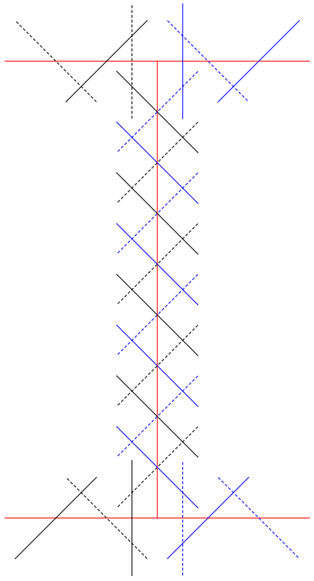
Figure 3. The segments $\sigma_{i,j}$ (in black) and $\sigma_{i+1,j}$ (in blue) on a shared edge (in red) of $\gamma_{i},\gamma_{i+1}$. As with Figure 2, for simplicity, we assume $N=9$.

Now for each $j\in\{1,\dots,2(c_{i}+1)N\}$ we define a copy $\tau_{i,j}$ of $\gamma$ in $\mathbb{R}^{3}$, scaled down by a factor of $8\sqrt{2}(5N)^{-1}$ with the following rules:

1. The projection of $\tau_{i,j}$ onto $\mathbb{R}^{2}\times\{0\}$ is the segment $\sigma_{i,j}$.

2. If $j$ is odd, then the projection of $\tau_{i,j}$ onto the $z$-axis is the segment

   $$\{(0,0)\}\times[(-4C_{g}-1)\tfrac{\sqrt{2}}{5N},(4C_{g}-1)\tfrac{\sqrt{2}}{5N}].$$

3. If $j$ is even, then the projection of $\tau_{i,j}$ onto the $z$-axis is the segment

   $$\{(0,0)\}\times[(-4C_{g}+1)\tfrac{\sqrt{2}}{5N}+\sqrt{2}(5N)^{-1},(4C_{g}+1)\tfrac{\sqrt{2}}{5N}].$$

For each $i\in\{1,\dots,g\}$ and $j\in\{1,\dots,2(c_{i}+1)N\}$, we let $\psi_{i,j}:\mathbb{R}^{3}\to\mathbb{R}^{3}$ be a similarity with scaling factor $8\sqrt{2}(5N)^{-1}$ such that $\psi_{i,j}(\gamma)=\tau_{i,j}$, and the image of the left edge of $\gamma$ is mapped to the edge of $\tau_{i,j}$, parallel to the $xy$-plane and with the highest third coordinate.

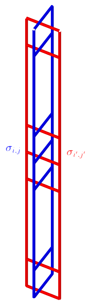
Figure 4. The two curves $\sigma_{i,j}$ and $\sigma_{i^{\prime},j^{\prime}}$ linked. Here we have chosen $g=6$.

Lemma 3.3.

Let $i,i^{\prime}\in\{1,\dots,g\}$, $j\in\{1,\dots,2(c_{i}+1)N\}$, and $j^{\prime}\in\{1,\dots,2(c_{i^{\prime}}+1)N\}$ with $(i,j)\neq(i^{\prime},j^{\prime})$.

1. We have that $\operatorname{dist}(\tau_{i,j},\tau_{i^{\prime},j^{\prime}})\geq 3(10N)^{-1}$.

2. For all $x\in\tau_{i,j}$ we have that $\operatorname{dist}(x,\gamma_{i})\leq(8C_{g}+6)\sqrt{2}(5N)^{-1}$.

3. We have that $\tau_{i,j}$ is linked with $\tau_{i^{\prime},j^{\prime}}$ if and only if $\sigma_{i,j}\cap\sigma_{i^{\prime},j^{\prime}}\neq\emptyset$. In the case they are linked, we have that $\psi_{i,j}(\gamma_{k})$ is linked with $\psi_{i^{\prime},j^{\prime}}(\gamma_{k})$.

Proof.

For the first claim, if $\sigma_{i,j}\cap\sigma_{i^{\prime},j^{\prime}}=\emptyset$, then by Lemma 3.2, (and given that $\sigma_{i,j},\sigma_{i^{\prime},j^{\prime}}$ are the projections of $\tau_{i,j},\tau_{i^{\prime},j^{\prime}}$ onto $\mathbb{R}^{2}\times\{0\}$, respectively) we have that

$$\operatorname{dist}(\tau_{i,j},\tau_{i^{\prime},j^{\prime}})\geq\operatorname{dist}(\sigma_{i,j},\sigma_{i^{\prime},j^{\prime}})\geq\sqrt{2}(5N)^{-1}.$$

If $\sigma_{i,j}\cap\sigma_{i^{\prime},j^{\prime}}\neq\emptyset$, then by Lemma 3.2 there are two possible cases. In either of these two cases, elementary calculations show that

$$\operatorname{dist}(\tau_{i,j},\tau_{i^{\prime},j^{\prime}})\geq\min\{3(10N)^{-1},2\sqrt{2}(5N)^{-1}\}=3(10N)^{-1}.$$

For the second claim, we have that for all $x\in\tau_{i,j}$

$$\operatorname{dist}(x,\gamma_{i})\leq|x_{i,j}-x| \leq\tfrac{1}{2}\operatorname{diam}{\sigma_{i,j}}+8C_{g}\sqrt{2}(5N)^{-1}+2\sqrt{2}(5N)^{-1}$$

$$=(8c+6)\sqrt{2}(5N)^{-1}.$$

For the third claim, it is easy to see that if $\sigma_{i,j}\cap\sigma_{i^{\prime},j^{\prime}}\neq\emptyset$, then $\sigma_{i,j}$ meets $\sigma_{i^{\prime},j^{\prime}}$ orthogonally and $\psi_{i,j}(\gamma_{k})$ is a copy of $\psi_{i^{\prime},j^{\prime}}(\gamma_{k})$ translated by a quarter of the length of its shortest side. Therefore, $\psi_{i,j}(\gamma_{k})$ is linked with $\psi_{i^{\prime},j^{\prime}}(\gamma_{k})$. Assume now that $\sigma_{i,j}\cap\sigma_{i^{\prime},j^{\prime}}=\emptyset$. Then, by Lemma 3.2 we have that $\tau_{i,j}\subset\sigma_{i,j}\times\mathbb{R}$, $\tau_{i^{\prime},j^{\prime}}\subset\sigma_{i^{\prime},j^{\prime}}\times\mathbb{R}$ with the two infinite strips having positive distance. Therefore, $\tau_{i,j}$ is not linked with $\tau_{i^{\prime},j^{\prime}}$. ∎

3.4. A Cantor set

Define the metric $\delta$ on $\mathbb{R}^{3}$

(3.3) $$\delta((x_{1},y_{1},z_{1}),(x_{2},y_{2},z_{2}))=\sqrt{\max\{|x_{1}-x_{2}|^{2},|y_{1}-y_{2}|^{2}\})+|z_{1}-z_{2}|^{2}}$$

and define the solid $g$-torus

$$T^{g}=\{p\in\mathbb{R}^{3}:\delta(p,\gamma)\leq 1/24\}.$$

Note that $T^{g}$ is the same as the usual neighborhood $\overline{B}(\gamma,\tfrac{1}{24})$ of $\gamma$ apart from the fact that the boundary of $T^{g}$ around the four corners of $\gamma_{0}$ has corners itself; see Figure 5.

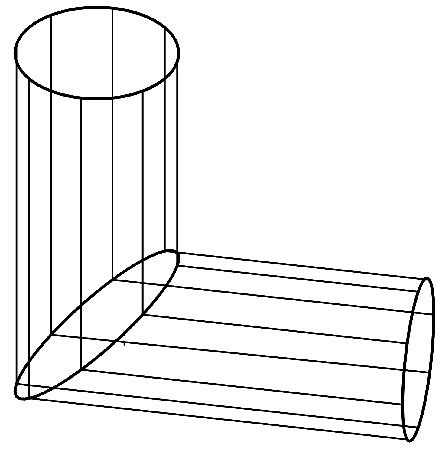
Figure 5.

By the choice of $N$ and Lemma 3.3(2), we have $\psi_{i,j}\left(T^{g}\right)\subset T^{g}$ for all $i\in\{1,\dots,g\}$ and all $j\in\{1,\dots,2(c_{i}+1)N\}$. By Lemma 3.3(1), we have $\psi_{i,j}\left(T^{g}\right)\cap\psi_{i,j}\left(T^{g}\right)=\emptyset$ for all $i,i^{\prime}\in\{1,\dots,g\}$, all $j\in\{1,\dots,2(c_{i}+1)N\}$, and $j^{\prime}\in\{1,\dots,2(c_{i^{\prime}}+1)N\}$ with $(i,j)\neq(i^{\prime},j^{\prime})$.

Let

(3.4) $$\{\phi_{1},\dots,\phi_{m}\}=\{\psi_{i,j}:i=1,\dots,g,\quad j=1,\dots,2(c_{i}+1)N\}$$

with $m=2(C_{g}+g)N$ and set

$$T^{1}_{g,i}=\{p\in\mathbb{R}^{3}:\delta(p,\gamma_{i})\leq 1/24\},\quad\gamma_{1,j}^{i}=\phi_{j}(\gamma_{i}),\quad T^{1}_{i,j}=\phi_{j}(T^{1}_{g,i}).$$

Define now the Cantor set

(3.5) $$X_{g}=\bigcap_{n=1}^{\infty}\bigcup_{j_{1},\dots,j_{n}\in\{1,\dots,m\}}\phi_{j_{1}}\circ\cdots\circ\phi_{j_{n}}(T^{g}).$$

4. Proving the genus is $g$

The goal of this section is to prove the following proposition.

Proposition 4.1.

The genus of $X_{g}$ is equal to $g$. Moreover, for each $x\in X_{g}$, the local genus $g_{x}(X_{g})=g$.

We start by establishing some terminology.

Definition 4.2.

Let $g\geq 1$. We say that a solid genus $g$ torus $T$ embedded in $\mathbb{R}^{3}$ is unknotted if $T$ is ambiently homeomorphic via $h$ to a solid torus $T_{0}$ with a planar core curve

(4.1) $$\left([0,g]\times\{0,1\}\right)\cup\left(\{0,1,\ldots,g\}\times[0,1]\right).$$

For $m\in\{1,\ldots,g\}$, let $\gamma^{T_{0}}_{m}$ be the loop in the core curve of $T_{0}$ given by

$$\gamma^{T_{0}}_{m}=\left([m-1,m]\times\{0,1\}\right)\cup\left(\{m-1,m\}\times[0,1]\right),$$

and set

$$\gamma^{T}_{m}=h^{-1}(\gamma^{T_{0}}_{m}).$$

See Figure 1 for an example of the core curve of an unknotted solid torus.

Definition 4.3.

Suppose that $T$ and $S$ are disjoint unknotted solid genus $g$ tori in $\mathbb{R}^{3}$. We say that $T$ and $S$ are completely linked if for $m\in\{1,\ldots,g\}$, $\gamma^{T}_{m}$ forms a Hopf link with $\gamma^{S}_{m}$ and is unlinked with $\gamma^{S}_{k}$ for $k\neq m$.

See Figure 4 for an example of completely linked solid genus $g$ tori.

Lemma 4.4.

Let $g\geq 1$ and let $T$ and $S$ be disjoint completely linked solid genus $g$ tori. If $U$ is a solid genus $g-1$ torus with $T\subset U$ and $\partial S\cap\partial U=\emptyset$, then $S\subset U$.

Note that this lemma may also be applied to core curves of solid tori, not just the solid tori themselves.

Proof.

Suppose for a contradiction that $S\subset\mathbb{R}^{3}\setminus U$. As $\pi_{1}(U)$ is the free group on $g-1$ generators, this group has rank $g-1$.

Let $\Gamma_{1}$ be the subgroup of $\pi_{1}(U)$ generated by $[\gamma^{T}_{1}]$, the equivalence class of $\gamma^{T}_{1}$. As $\gamma^{T}_{1}\subset T$ is linked with $\gamma^{S}_{1}\subset S^{3}\setminus U$, it follows that $[\gamma^{T}_{1}]$ is non-trivial in $\pi_{1}(U)$. Hence $\Gamma_{1}$ has rank $1$.

For $k\in\{1,\ldots,g-1\}$, suppose that the subgroup $\Gamma_{k}$ of $\pi_{1}(U)$ is generated by $[\gamma^{T}_{1}],\ldots,[\gamma^{T}_{k}]$ has rank $k$. Every element of $\Gamma_{k}$ can be represented by a loop that does not link with $\gamma^{S}_{k+1}$. As $\gamma^{S}_{k+1}\subset\mathbb{R}^{3}\setminus U$, this also holds for every element of $\Gamma_{k}$. As $\gamma^{T}_{k+1}$ is linked with $\gamma^{S}_{k+1}\subset\mathbb{R}^{3}\setminus U$, it follows that $[\gamma^{T}_{k+1}]$ is both non-trivial in $\pi_{1}(U)$ and not an element of $\Gamma_{k}$. It follows that $\Gamma_{k+1}$ has rank $k+1$.

By induction, we conclude that $\Gamma_{g}$ is a rank $g$ subgroup of $\pi_{1}(U)$, which contradicts the fact that $\pi_{1}(U)$ has rank $g-1$. ∎

Next, if $\gamma$ is an unknotted circle in $\mathbb{R}^{3}$, then it bounds a topological disk. Any such disk is called a filling disk. In the special case where $\gamma$ is a planar topological circle, there is a unique filling disk which lies in the same plane as $\gamma$. This is called the canonical filling disk for $\gamma$.

Definition 4.5.

If $T$ is a solid unknotted genus $g$ torus with ambient homeomorphism $h:T\to T_{0}$ where $T_{0}$ has core curve given by (4.1), then we say that $T$ has a nice collection of filling disks if for each $m$ the filling disk for $\gamma^{T}_{m}$ arises as the image of a canonical filling disk for $\gamma^{T_{0}}_{m}$ under $h^{-1}$.

Evidently, a nice collection of filling disks for $T$ consists of a collection of pairwise disjoint filling disks and so that if $\sigma_{1},\sigma_{2}$ are any two closed loops contained in different filling disks, then $\sigma_{1},\sigma_{2}$ are unlinked.

Lemma 4.6.

Let $g\geq 1$ and let $T$ and $S$ be disjoint completely linked genus $g$ tori with core curves $\gamma^{T}_{k},\gamma^{S}_{k}$ respectively, for $k\in\{1,\ldots,g\}$. Let $D^{S}_{m}$, for $m\in\{1,\ldots,g\}$, be a nice collection of filling disks for $\gamma^{S}_{m}$. Let $U\subset\mathbb{R}^{3}$ be a solid genus $g-1$ torus.

1. If $T\cup S\subset U$, then there exists a path in $U$ joining $T$ and $S$ contained in one of the filling disks $D^{S}_{m}$ for some $m\in\{1,\ldots,g\}$.

2. If $T\cup S\subset\mathbb{R}^{3}\setminus U$, then there exists a path in $\mathbb{R}^{3}\setminus U$ joining $T$ and $S$ contained in one of the filling disks $D^{S}_{m}$ for some $m\in\{1,\ldots,g\}$.

Again, this lemma may be applied to core curves of solid tori.

Proof.

Suppose first that $T\cup S\subset U$. For a contradiction, suppose that for each $m\in\{1,\ldots,g\}$, there is a loop $\sigma_{m}\subset D^{S}_{m}\cap(\mathbb{R}^{3}\setminus U)$ which separates $\gamma^{S}_{m}$ from $D^{S}_{m}\cap\gamma^{T}_{m}$ in $D^{S}_{m}$. As $D^{S}_{m}$ is a nice collection of filling disks, these loops $\sigma_{m}$ are pairwise unlinked.

As in the proof of Lemma 4.4, we consider the subgroups $\Gamma_{m}$ of $\pi_{1}(U)$ generated by $[\gamma^{T}_{1}],\ldots,[\gamma^{T}_{m}]$. As $\gamma^{T}_{1}$ is linked with $\sigma_{1}\subset\mathbb{R}^{3}\setminus U$, it follows that $\Gamma_{1}$ has rank $1$. The same inductive argument as above, with $\sigma_{m}$ in place of $\gamma^{S}_{m}$, shows that $\Gamma_{m}$ has rank $m$ for $m\in\{1,\ldots,g\}$. This again contradicts the fact that $\pi_{1}(U)$ has rank $g-1$ and proves (i).

Next suppose that $T\cup S\subset\mathbb{R}^{3}\setminus U$. For a contradiction, suppose that for $m\in\{1,\ldots,g\}$, there is a loop $\nu_{m}\subset D^{S}_{m}\cap U$ which separates $\gamma^{S}_{m}$ from $D^{S}_{m}\cap\gamma^{T}_{m}$ in $D^{S}_{m}$. As $D^{S}_{m}$ is a nice collection of filling disks, these loops $\nu_{m}$ are pairwise unlinked.

As in part (i), we consider the subgroups $\Gamma_{m}$ of $\pi_{1}(U)$ generated by $[\nu_{1}],\ldots,[\nu_{m}]$. As $\nu_{m}\subset U$ is linked with $\gamma^{T}_{m}\in\mathbb{R}^{3}\setminus U$ and unlinked with $\gamma^{T}_{k}$ for $k\neq m$, it follows as above that $\Gamma_{m}$ has rank $m$. Hence $\Gamma_{g}$ is a rank $g$ subgroup of the rank $g-1$ group $\pi_{1}(U)$ which is a contradiction and proves (ii). ∎

Recall the construction of the Cantor set $X_{g}$ from (3.5). Evidently $\operatorname{diam}X_{g}>0$. The construction of $X_{g}$ yields a defining sequence given by, for $n\geq 1$,

$$M_{n}=\bigcup_{j_{1},\ldots,j_{n}\in\{1,\ldots,m\}}\phi_{j_{1}}\circ\cdots\circ\phi_{j_{n}}(T^{g}).$$

We fix some notation. Given an integer $k\geq 0$, we denote by $\{1,\ldots,m\}^{k}$ the set of words formed from the alphabet $\{1,\ldots,m\}$ that have length exactly $k$. Conventionally, we set $\{1,\ldots,m\}^{0}=\{\varepsilon\}$ where $\varepsilon$ is the empty word. We also denote by $\{1,\ldots,m\}^{*}=\bigcup_{k\geq 0}\{1,\ldots,m\}^{k}$ the set of all finite words formed from $\{1,\ldots,m\}$. For $k\geq 1$, denote by $\kappa:\{1,\ldots,m\}^{k}\to\{1,\ldots,m\}^{k-1}$ the forgetful map defined by

$$\kappa(j_{1}\cdots j_{k})=j_{1}\ldots j_{k-1}$$

with $\kappa(j)=\varepsilon$ for $j\in\{1,\ldots,m\}$. We have the alternative description of the defining sequence

$$M_{n}=\bigcup_{w\in\{1,\ldots,m\}^{n}}\phi_{w}(T^{g}).$$

Here, if $w=j_{1}\ldots j_{n}$ then $\phi_{w}=\phi_{j_{1}}\circ\cdots\circ\phi_{j_{n}}$.

We are now in a position to prove that the genus of $X_{g}$ is $g$.

Proof of Proposition 4.1.

The construction of $X_{g}$ shows that its genus is at most $g$.

Suppose for a contradiction that the genus of $X_{g}$ is strictly smaller than $g$. Then we can find an alternative defining sequence $\widetilde{M}_{n}$ which contains solid genus $g-1$ tori of arbitrarily small diameter. Choose a solid genus $g-1$ torus $U\subset\widetilde{M}$ of diameter at most $\alpha^{2}\operatorname{diam}(X^{g})$, where $\alpha=8\sqrt{2}(5N)^{-1}$ is the scaling factor of each $\phi_{j}$.

As $U$ is a solid torus with $\partial U\subset\mathbb{R}^{3}\setminus X_{g}$, we have $\operatorname{dist}(\partial U,X_{g})=\delta>0$. As $\operatorname{dist}(\partial M_{n},X_{g})\to 0$ as $n\to\infty$, it follows that we may choose $p\in\mathbb{N}$ so that $\partial U\cap\partial M_{p}=\emptyset$. It follows that every component of $M_{p}$ is either contained in $U$ or contained in $\mathbb{R}^{3}\setminus U$, and at least one is contained in $U$. We analyze what happens in either case.

Suppose $w\in\{1,\ldots,m\}^{p}$ and $\phi_{w}(T^{g})\subset U$. Then the collection of tori given by $\phi_{\kappa(w)k}(T^{g})$, for $k\in\{1,\ldots,m\}$, form a chain of linked tori contained in the larger torus $\phi_{\kappa(w)}(T^{g})$. As $\phi_{w}(T^{g})$ is contained in $U$, a repeated application of Lemma 4.4 shows that all of the tori $\phi_{\kappa(w)k}(T^{g})$ are contained in $U$, for $k\in\{1,\ldots,m\}$. As each component of the defining sequence $M_{p}$ has a planar core curve, it follows that we may consider a nice collection of filling disks for each $\phi_{\kappa(w)k}(T^{g})$ consisting of canonical filling disks. Then a repeated application of Lemma 4.6 (i) shows that we may construct a path $C_{\kappa(w)}\subset U\cap(\phi_{\kappa(w)}(T^{g}))$ which is a core curve of $\phi_{\kappa(w)}(T^{g})$ and consists of line segments from the core curves of $\phi_{\kappa(w)k}(T^{g})$ and paths in the canonical filling disks of the $\phi_{\kappa(w)k}(T^{g})$.

On the other hand, suppose that $w\in\{1,\ldots,m\}^{p}$ and $\phi_{w}(T^{g})\subset\mathbb{R}^{3}\setminus U$. Then an analogous repeated application of Lemma 4.4 and Lemma 4.6 (ii) shows that there is a path $C_{\kappa(w)}\subset(\mathbb{R}^{3}\setminus U)\cap(\phi_{\kappa(w)}(T^{g}))$ which is a core curve of $\phi_{\kappa(w)}(T^{g})$.

The conclusion from the above argument is that if $\phi_{w}(T^{g})$ is in $U$ (respectively is in $\mathbb{R}^{3}\setminus U$), then the chain

$$\bigcup_{k\in\{1,\ldots,m\}}\phi_{\kappa(w)k}(T^{g})$$

is contained in $U$ (respectively is contained in $\mathbb{R}^{3}\setminus U$), and we may find a core curve $C_{\kappa(w)}$ for $\phi_{\kappa(w)}(T^{g})$ which is contained in $U$ (respectively contained in $\mathbb{R}^{3}\setminus U$).

We may now repeat this argument. For $q\in\{1,\ldots,g-1\}$ and $v\in\{1,\ldots,m\}^{p-q}$, suppose that we have all core curves $C_{v}$ for $\phi_{v}(T^{g})$ either contained in $U$ or contained in $\mathbb{R}^{3}\setminus U$. Suppose also that we have a nice collection of filling disks for each $\phi_{v}(T^{g})$ that are contained in $\phi_{\kappa(v)}(T^{g})$.

If $\phi_{v}(T^{g})\subset U$, then a repeated application of Lemma 4.4 shows that $\phi_{\kappa(v)k}(T^{g})$ is contained in $U$ for all $k\in\{1,\ldots,m\}$. Then a repeated application of Lemma 4.6 may be used to construct a path in $\phi_{\kappa(v)}(T^{g})$ which is a core curve for $\phi_{\kappa(v)}(T^{g})$ and is contained in $U$. On the other hand, if $\phi_{v}(T^{g})\subset\mathbb{R}^{3}\setminus U$, then an analogous argument yields a path in $\phi_{v}(T^{g})$ which is a core curve for $\phi_{\kappa(v)}(T^{g})$ and is contained in $\mathbb{R}^{3}\setminus U$.

To finish, for some $w\in\{1,\ldots,m\}^{p}$, there exists a component $\phi_{w}(T^{g})$ of $M_{p}$ which is contained in $U$. Applying the argument above inductively $p$ times, we obtain a core curve $C_{\kappa^{p}(w)}(T^{g})=C_{\varepsilon}(T^{g})$ of $T^{g}$ itself which is contained in $U$. This forces $\operatorname{diam}U\geq\operatorname{diam}(X^{g})$ which contradicts $\operatorname{diam}(U)<\alpha^{2}\operatorname{diam}(X^{g})$.

The argument above shows that we cannot insert a genus $g-1$ handlebody into a defining sequence for $X_{g}$ in any non-trivial way. From this we conclude that the local genus of $X_{g}$ is $g$ at every $x\in X_{g}$. ∎

5. A Julia set of genus $g$

The goal of this section is to construct a UQR map of $\overline{\mathbb{R}^{3}}$ that has $X_{g}$ as its Julia set. This along with Proposition 4.1, completes the proof of Theorem 1.1.

5.1. A basic covering map

For each $n\in\mathbb{N}$ we denote by $\Sigma^{n}$ the associated planar curve ${\gamma}$ from Section 3.2 for the genus $n$, and by $\Gamma_{n,i}$ the simple closed curves ${\gamma}_{i}$ defined in (3.2). Fix for the rest of this section an integer $g\in\mathbb{N}$ and let $N_{g}$ be the integer defined in (3.1).

For each $n\in\{1,\dots,g\}$, each $i\in\{1,\dots,n\}$ and each $j\in\{1,\dots,(2c_{n,i}+2)N_{g}\}$ denote by $\alpha_{n,i,j}$ the planar segments $\sigma_{i,j}$ of length $8\sqrt{2}(5N_{g})^{-1}$ intersecting $\Gamma_{n,i}$ as defined in Section 3.3. Define also $\Sigma^{g}_{n,i,j}$ to be the curves $\tau_{i,j}$ defined just before Lemma 3.3 which are copies of $\Sigma^{g}$ scaled down by a factor of $8\sqrt{2}(5N_{g})^{-1}$ and their projection on $\mathbb{R}^{2}\times\{0\}$ are the segments $\alpha_{n,i,j}$.

Recall the metric $\delta$ from (3.3). Define for each $n\in\{1,\dots,g\}$,

$$T^{n}=\{p\in\mathbb{R}^{3}:\delta(p,\Sigma^{n})\leq\tfrac{1}{24}\}$$

and for each $i\in\{1,\dots,n\}$ and each $j\in\{1,\dots,(2c_{n,i}+2)N_{g}\}$

$$T^{g}_{n,i,j}=\{p\in\mathbb{R}^{3}:\delta(p,\Sigma^{g}_{n,i,j})\leq\sqrt{2}(15N_{g})^{-1}\}.$$

The goal of this section is to construct the following map.

Proposition 5.1.

There exists a degree $2^{\lceil\log_{2}{g}\rceil+2}N_{g}$ BLD cover

$$F:T^{g}\setminus\bigcup_{i,j}\operatorname{int}(T^{g}_{g,i,j})\to\overline{B}(0,2C_{g,g})\setminus\operatorname{int}(T^{g})$$

such that $F(\partial T^{g}_{g,i,j})=\partial T^{g}$ for each $i,j$.

The first step is given in the following lemma.

Lemma 5.2.

For each $n\in\{2,\dots,g\}$ there exists a degree 2 BLD cover

$$F_{n}:T^{n}\setminus\bigcup_{i,j}\operatorname{int}(T^{g}_{n,i,j})\to T^{\lceil\frac{n}{2}\rceil}\setminus\bigcup_{i,j}\operatorname{int}(T^{g}_{\lceil\frac{n}{2}\rceil,i,j})$$

such that for each $i,j$ there exist $i^{\prime},j^{\prime}$ with $F_{n}(\partial T^{g}_{n,i,j})=\partial T^{g}_{\lceil\frac{n}{2}\rceil,i^{\prime},j^{\prime}}$.

Proof of Lemma 5.2.

The construction of $F_{n}$ is different for the cases that $n$ is even or odd.

Assume first that $n=2k$ for some $k\in\mathbb{N}$. Let

$$\iota_{1}:\mathbb{R}^{3}\to\mathbb{R}^{3}\qquad\text{with}\quad\iota_{1}(x,y,z)=(2C_{2k,k}-x,y,-z)$$

be the $\pi$-degree rotation with respect to the line $\ell_{1}=\{z=0\}\cap\{x=C_{2k,k}\}$. By the construction of the sequence $(a_{n,i})_{i=1}^{n}$ and the construction of sets $(T^{g}_{2k,i,j})_{i,j}$ we have that sets $T^{2k}$ and $\bigcup_{i,j}T^{g}_{2k,i,j}$ are both invariant under $\iota_{1}$ since both sets are symmetric with respect to the line $\ell_{1}$. The quotient map $q:T^{2k}\to T^{2k}/\langle\iota_{1}\rangle$ is a degree 2 sense-preserving map satisfying

1. $q(T^{2k})$ is the image of $T^{k}$ under a bi-Lipschitz homeomorphism of $\mathbb{R}^{3}$;

2. for each $j$ there exists $j^{\prime}$ such that $q(T^{g}_{2k,i,j})=q(T^{g}_{2k,2k-i,j^{\prime}})$;

3. for each $i,j$, the image $q(T^{g}_{2k,i,j})$ is the image of $T^{g}_{2k,i,j}$ under a bi-Lipschitz homeomorphism of $\mathbb{R}^{3}$.

To obtain a BLD cover, we consider a PL version of $q$. Give $T^{2k}$ a $C^{1}$-triangulation $\zeta:|U|\to T^{2k}$ in the sense of [Mun66, 16, p. 81] by a simplicial complex $U$ in $\mathbb{R}^{3}$ that respects the involution $\iota_{1}|T^{2k}$ and of which $\zeta^{-1}(\bigcup_{i,j}(T^{g}_{2k,i,j}))$ is a subcomplex. Identify $q(T^{2k})$ with a simplicial complex $V$ via $\xi:|V|\to q(T^{2k})$ in $\mathbb{R}^{3}$ of which $q(\bigcup_{i,j}(T^{g}_{2k,i,j}))$ is a subcomplex such that $q\circ\zeta:U\to q(T^{2k})$ is simplicial. Under these identifications, $q$ is a BLD map.

Suppose now that $n=2k+1$. Recall that $c_{2k+1,k+1}=3$, $c_{k+1,k+1}=1$. We decompose $T^{2k+1}\setminus\bigcup_{i,j}\operatorname{int}(T^{g}_{2k+1,i,j})$ into six pieces and we decompose $T^{k+1}\setminus\bigcup_{i,j}\operatorname{int}(T^{g}_{k+1,i,j})$ into three pieces as follows. Let

$$U_{1} =(T^{2k+1}\setminus\bigcup_{i,j}\operatorname{int}(T^{g}_{2k+1,i,j}))\cap\{x\leq C_{2k+1,k}+\tfrac{1}{2}\}$$

$$U_{2} =(T^{2k+1}\setminus\bigcup_{i,j}\operatorname{int}(T^{g}_{2k+1,i,j}))\cap\{C_{2k+1,k}+\tfrac{3}{4}\leq x\leq C_{2k+1,k}+\tfrac{3}{2}\}\cap\{y\geq\tfrac{1}{2}\}$$

$$U_{3} =(T^{2k+1}\setminus\bigcup_{i,j}\operatorname{int}(T^{g}_{2k+1,i,j}))\cap\{C_{2k+1,k}+\tfrac{3}{2}\leq x\leq C_{2k+1,k}+\tfrac{9}{4}\}\cap\{y\geq\tfrac{1}{2}\}$$

$$U_{4} =(T^{2k+1}\setminus\bigcup_{i,j}\operatorname{int}(T^{g}_{2k+1,i,j}))\cap\{C_{2k+1,k}+\tfrac{3}{4}\leq x\leq C_{2k+1,k}+\tfrac{3}{2}\}\cap\{y\leq\tfrac{1}{2}\}$$

$$U_{5} =(T^{2k+1}\setminus\bigcup_{i,j}\operatorname{int}(T^{g}_{2k+1,i,j}))\cap\{C_{2k+1,k}+\tfrac{3}{2}\leq x\leq C_{2k+1,k}+\tfrac{9}{4}\}\cap\{y\leq\tfrac{1}{2}\}$$

$$U_{6} =(T^{2k+1}\setminus\bigcup_{i,j}\operatorname{int}(T^{g}_{2k+1,i,j}))\cap\{x\geq C_{2k+1,k}+\tfrac{9}{4}\}.$$

Let also

$$V_{1} =(T^{k+1}\setminus\bigcup_{i,j}T^{g}_{k+1,i,j})\cap\{x\leq C_{k+1,k}+\tfrac{1}{2}\}$$

$$V_{2} =(T^{k+1}\setminus\bigcup_{i,j}T^{g}_{k+1,i,j})\cap\{x\geq C_{k+1,k}+\tfrac{1}{2}\}\cap\{y\geq\tfrac{1}{2}\}$$

$$V_{3} =(T^{k+1}\setminus\bigcup_{i,j}T^{g}_{k+1,i,j})\cap\{x\geq C_{k+1,k}+\tfrac{1}{2}\}\cap\{y\leq\tfrac{1}{2}\}.$$

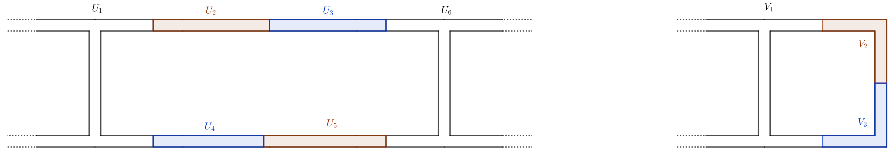
Figure 6. The decompositions of $T^{2k+1}$ (left) and of $T^{k+1}$ (right). For simplicity we have omitted the sets $T^{g}_{2k+1,i,j}$ and $T^{g}_{k+1,i,j}$.

Let

$$\iota_{2}:\mathbb{R}^{3}\to\mathbb{R}^{3}\qquad\text{with}\quad\iota_{2}(x,y,z)=(2C_{2k+1,k}+\tfrac{3}{2}-x,1-y,z)$$

be the $\pi$-degree rotation with respect to the line $\{y=1/2\}\cap\{x=C_{2k+1,k}+\tfrac{3}{2}\}$ and let

$$\iota_{3}:\mathbb{R}^{3}\to\mathbb{R}^{3}\qquad\text{with}\quad\iota_{3}(x,y,z)=(y+C_{k+1,k},C_{k+1,k+1}-x,z)$$

be the $\pi/2$-degree rotation with respect to the line $\{y=1/2\}\cap\{x=C_{k+1,k}+\tfrac{1}{2}\}$.

Define $F_{2k+1}|U_{1}=\text{Id}$ (which maps $U_{1}$ onto $V_{1}$) and $F_{2k+1}|U_{6}=\iota_{2}$ (which maps $U_{6}$ onto $V_{1}$). We claim that there exists a bi-Lipschitz homeomorphism $h:U_{2}\to V_{2}$ such that

1. for each $j$, there exists unique $j^{\prime}$ such that $h|\partial T^{g}_{2k+1,k+1,j}$ is an isometry mapping $\partial T^{g}_{2k+1,k+1,j}$ onto $\partial T^{g}_{k+1,k+1,j^{\prime}}$;

2. $h|\partial U_{1}\cap\partial U_{2}=\text{Id}$ and $h|\partial U_{3}\cap\partial U_{2}=\iota_{2}$.

The construction of $h$ is elementary but tedious and we postpone its proof until Appendix A. Assuming the existence of $h$, we define

1. $F_{2k+1}|U_{2}=h$ (which maps $U_{2}$ onto $V_{3}$),

2. $F_{2k+1}|U_{3}=\iota_{3}\circ h(x-\tfrac{3}{4},y,z)$ (which maps $U_{3}$ onto $V_{3}$),

3. $F_{2k+1}|U_{4}=(F_{2k+1}|U_{3})\circ\iota_{2}$ (which maps $U_{4}$ onto $V_{3}$), and

4. $F_{2k+1}|U_{5}=(F_{2k+1}|U_{2})\circ\iota_{2}$ (which maps $U_{5}$ onto $V_{2}$).

It is easy to see that $F_{2k+1}$ is a degree 2 BLD cover. ∎

We are now ready to prove Proposition 5.1. The proof follows the arguments in [FS22, §4.1] almost verbatim.

Proof of Proposition 5.1.

Applying Lemma 5.2 a total of $\lceil\log_{2}{g}\rceil$ many times, we obtain a degree $2^{\lceil\log_{2}{g}\rceil}$ BLD map

$$G:T^{g}\setminus\bigcup_{i,j}\operatorname{int}(T^{g}_{q,i,j})\to T^{1}\setminus\bigcup_{j=1}^{4N_{g}}\operatorname{int}(T^{g}_{1,1,j})$$

such that for each $i,j$ there exist $i^{\prime},j^{\prime}$ with $G(\partial T^{g}_{g,i,j})=\partial T^{g}_{1,i^{\prime},j^{\prime}}$.

It remains to construct a degree $4N_{g}$ BLD map

$$T^{1}\setminus\bigcup_{j=1}^{4N_{g}}\operatorname{int}(T^{g}_{1,1,j})\to\overline{B}(0,2C_{g,g})\setminus\operatorname{int}(T^{g}).$$

We apply a bi-Lipschitz map $\Phi:T^{1}\to T^{1}$ that modifies $T^{1}$ in two ways. Firstly, we translate $T^{1}$ so that its core curve ${\gamma}_{1}$ is the 2-dimensional unit square

$$\{(x,y,z):z=0,\quad\max\{|x|,|y|\}=1\}.$$

Then, we apply a bi-Lipschitz map that is radial with respect to the $z$-axis so that

1. the core curve ${\gamma}_{0}^{1}$ traced by the chain $\bigcup_{j=1}^{4N_{g}}\operatorname{int}(T^{g}_{1,1,j})$ is a circle in the $xy$-plane centered at the origin;

2. every cross section of $T^{1}$ taken perpendicular to the above core curve is a geometric disk.

Additionally, we deform $\text{int}(T^{1})$ so that all the sets $T^{g}_{1,1,1},\dots,T^{g}_{1,1,4N_{g}}$ satisfy

$$\rho(T^{g}_{1,1,j})=\rho(T^{g}_{1,1,j+2})\quad\text{for $j\in\{1,\dots,4N_{g}\}$}$$

(with the convention $T^{g}_{1,1,4N_{g}+1}=T^{g}_{1,1,1}$ and $T^{g}_{1,1,4N_{g}+2}=T^{g}_{1,1,2}$) where $\rho$ is the rotation about the $z$-axis by an angle $2\pi/N_{g}$,

$$\rho(r,\theta,z)=(r,\theta+4\pi/N_{g},z).$$

This deformation is made to preserve the fact that all $T^{g}_{1,1,j}$ remain geometrically similar to each other. Finally, if necessary, rotate $T^{1}$ around the $z$-axis to ensure that the set $\bigcup_{j=1}^{4N_{g}}\operatorname{int}(T^{g}_{1,1,j})$ is symmetric with respect to a rotation about the $x$-axis by an angle $\pi$; see Figure 7. Abusing notation, we will write $T^{1}$ and $T^{g}_{1,1,i}$, instead of $\Phi(T^{1})$ and $\Phi(T^{g}_{1,1,i})$.

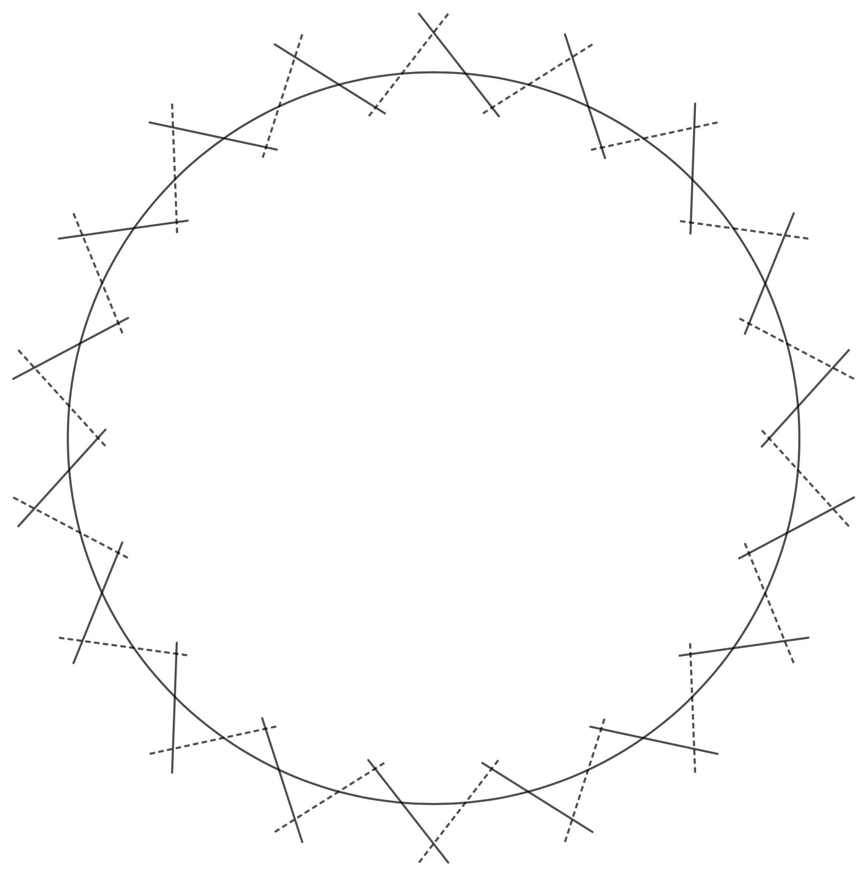
Figure 7. The projections of ${\gamma}_{1}$ (the core curve of $T^{1}$) and of $(T^{g}_{1,1,j})_{j=1}^{4N}$ on the $xy$-plane after applying the bi-Lipschitz deformation $q$. For simplicity we have chosen $N_{g}=9$.

Let $\omega:\mathbb{R}^{3}\to\mathbb{R}^{3}$ be the degree $2N_{g}$ winding map

$$\omega(r,\theta,z)=(r,2N_{g}\theta,z).$$

Then $\omega|T^{1}:T^{1}\to T^{1}$ is an unbranched cover that maps all $T^{g}_{1,1,j}$ with odd indices $j$ to $\omega(T^{g}_{1,1,1})$ and all $T^{g}_{1,1,j}$ with even indices $j$ to $\omega(T^{g}_{1,1,2})$. By construction, $\omega(T_{1,1,1}^{g})$ and $\omega(T^{g}_{1,1,2})$ are linked inside $T^{1}$ (see Figure 8) and are symmetric to each other via a rotation about the $x$-axis by an angle $\pi$. Let $\iota$ be the involution for the latter rotation, that is

$$\iota(x,y,z)=(x,-y,-z).$$

The quotient $q:T^{1}\to T^{1}/\langle\iota\rangle$ is a degree 2 sense preserving map under which $q(\omega(T^{g}_{1,1,1}))=q(\omega(T^{g}_{1,1,2}))$ is the image of $T^{g}$ under a bi-Lipschitz map of $\mathbb{R}^{3}$.

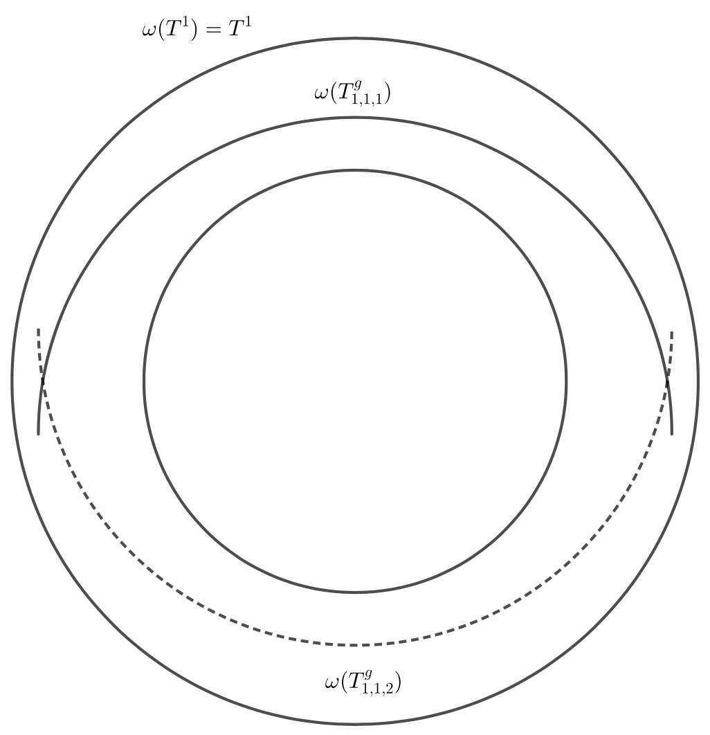
Figure 8.

Post-composing with more bi-Lipschitz deformations, the map $q\circ\omega\circ G$ is a degree $4N_{g}2^{\lceil\log_{2}{g}\rceil}$ branched cover from $T^{g}$ onto $\overline{B}(0,4)$ mapping each $T^{g}_{g,i,j}$ onto $T^{g}$. Following the arguments in the proof of Lemma 5.2 we can obtain a PL, and hence quasiregular, version of the map $q\circ\omega\circ G$. This completes the proof of the proposition. ∎

5.2. Construction of a UQR map

The construction of the UQR map of Theorem 1.1 follows closely the ideas in [FW15, Section 5] and [FS22, §4.2] so we only sketch the arguments. We require the following two results.

Theorem 5.3.

For every $d\in\mathbb{N}$ with $d>1$ and for every $n\in\mathbb{N}$, there is a UQR map $h:\overline{\mathbb{R}^{3}}\to\overline{\mathbb{R}^{3}}$ of degree $2^{n}d^{2}$ with Julia set $J(h)=\mathbb{S}^{2}$. In particular, for any $r>0$, $h(B(0,r))=B(0,r^{2^{n/2}d})$.

We defer the proof of this result to Appendix B. For the next theorem see also [HR02, Theorem 0.3], [PRW14, Theorem 3.1].

Theorem 5.4 ([BE79, Theorem 6.2]).

Let $W$ be a connected, compact, oriented PL 3-manifold in some $\mathbb{R}^{n}$ whose boundary $\partial W$ consists of two components $M_{0}$ and $M_{1}$ with the induced orientation. Let $W^{\prime}=N\setminus(\text{int}(B_{0})\cup\text{int}(B_{1}))$ be an oriented PL 3-sphere $N$ in $\mathbb{R}^{n}$ with two disjoint polyhedral 3-balls removed, and have the induced orientation on its boundary. Suppose that $\phi_{i}:M_{i}\to\partial B_{i}$ is a sense-preserving oriented branched cover of degree $d\geq 3$ for each $i=0,1$. Then there exists a sense-preserving PL branched cover $\phi:W\to W^{\prime}$ of degree $d$ that extends $\phi_{0}$ and $\phi_{1}$.

Recall the constant $C_{g,g}$ from §3.1 and set

$$R=(4C_{g,g})^{2\sqrt{N_{g}}2^{\frac{1}{2}\lceil\log_{2}{g}\rceil}}.$$

Let $B_{0}=B(0,4C_{g,g})$, $B_{-1}=B(0,R)$. We decompose $\mathbb{R}^{3}$ in two different ways:

$$\mathbb{R}^{3} =\left(\bigcup_{i,j}T^{g}_{g,i,j}\right)\cup\left(T^{g}\setminus\bigcup_{i,j}T^{g}_{g,i,j}\right)\cup(B_{0}\setminus T^{g})\cup(\mathbb{R}^{3}\setminus B_{0})$$

and

$$\mathbb{R}^{3} =T^{g}\cup(B_{0}\setminus T^{g})\cup(B_{-1}\setminus B_{0})\cup(\mathbb{R}^{3}\setminus B_{-1}).$$

Define now a map $f:\mathbb{R}^{3}\to\mathbb{R}^{3}$ in the following way.

1. Set

   $$f:T^{g}\setminus\bigcup_{i,j}\text{int}(T^{g}_{g,i,j})\to B_{0}\setminus\operatorname{int}(T^{g})$$

   to be the map of Proposition 5.1.

2. Extend $f$ to $\bigcup_{i,j}T^{g}_{g,i,j}$ by setting

   $$f|T^{g}_{g,i,j}=\psi_{i,j}^{-1}:T^{g}_{g,i,j}\to T^{g}.$$

   Recall the definitions of $\psi_{i,j}$ from §3.4.

3. Define $f:\mathbb{R}^{3}\setminus\text{int}(B_{0})\to\mathbb{R}^{3}\setminus\text{int}(B_{-1})$ to be the restriction of the UQR map of degree $2^{\lceil\log_{2}{g}\rceil}4N_{g}$ from Theorem 5.3. Note that $f|\mathbb{R}^{3}\setminus\text{int}(B_{0})$ is orientation preserving and maps $S(0,4C_{g,g})$ onto $S(0,R)$.

4. Since $f|\partial B_{0}$ is a BLD degree $2^{\lceil\log_{2}{g}\rceil}4N_{g}$ map onto $\partial B_{-1}$, and since $f|\partial T^{g}$ is also a degree $2^{\lceil\log_{2}{g}\rceil}4N_{g}$ BLD map onto $\partial B_{0}$, by Theorem 5.4 there exists a degree $2^{\lceil\log_{2}{g}\rceil}4N_{g}$ BLD extension $f:B_{0}\setminus\text{int}(T^{g})\to B_{-1}\setminus\text{int}(B_{0})$.

The map $f:\mathbb{R}^{3}\to\mathbb{R}^{3}$ defined above is UQR and of polynomial type [FS22, Lemma 4.1] (see also [FW15, Lemma 5.1]) and its Julia set is equal to $X_{g}$ [FS22, Lemma 4.2] (see also [FW15, Lemma 5.2]).

6. Genus and Julia sets

First in this section, we prove Theorem 1.2.

Proof of Theorem 1.2.

Apply Lemma 2.1 to find an $r_{1}$-neighbourhood of $U$ and $N\in\mathbb{N}$ such that $\overline{f^{-N}(U)}\subset U$. Replace $f$ with $F=f^{N}$. Then $J(F)=J(f)$ and $F$ is also hyperbolic. Moreover, if $x\in J(f)$, then $F^{-1}$ has $\deg(F)$ homeomorphic branches defined on $B(x,r_{1})$.

Next, find a defining sequence $(M_{i})_{i=0}^{\infty}$ for $J(F)$ and choose $I\in\mathbb{N}$ such that each component of $M_{I}$ is contained in an $r_{1}$ ball centred at some $x\in J(F)$. We construct a new defining sequence for $J(F)$ as follows. Set $N_{0}=M_{I}$ and then define $N_{k}=F^{-k}(N_{0})$ for $k\geq 1$. Since $F^{-k}$ has $\deg(F)^{k}$ homeomorphic branches on each $B(x,r_{1})$, for $x\in J(F)$, and each component of $N_{0}$ is contained in such a ball, it follows that the maximal genus of components of $N_{k}$ is equal to the maximal genus of components of $N_{0}$ for each $k\geq 1$. Denote this integer by $g_{0}$.

Since we have constructed a defining sequence for $J(F)$ with genus $g_{0}$, it follows that the genus of $J(F)$ is bounded above by $g_{0}$ and is, in particular, finite. ∎

Next, we prove Theorem 1.3.

Proof of Theorem 1.3.

By Theorem 1.2, the genus of $J(f)$ is finite. Since $g_{x}(J(f))\leq g(J(f))$ for any $x\in J(f)$, the local genus is also finite at every point. So suppose $g_{x}(J(f))=g$. In the definition for the local genus (recalling that $M_{i}^{x}$ is the component of $M_{i}$ containing $x$) in Definition 2.3, we may replace $\inf$ by $\min$. In particular, there exists a defining sequence $(M_{i})_{i=0}^{\infty}$ for which $g(M_{i}^{x})=g$ for all $i$, by adding extra handles if necessary. We may also assume that each $M_{i}^{x}$ is contained in $B(x,r_{1})$, recalling Lemma 2.1.

Suppose $y=f(x)$. Then for each $i$, $f(M_{i}^{x})$ is a solid genus $g$ handlebody with boundary in $F(f)$. Further, we have

$$\bigcap_{i=1}^{\infty}f(M_{i}^{x})=\{y\}.$$

It follows that the local genus of $y$ is bounded above by $g$. Towards a contradiction, suppose that $g_{y}(J(f))=g^{\prime}<g$. Then, arguing as above, we may find a defining sequence $(N_{j})_{j=1}^{\infty}$ such that $N_{j}^{y}$ is a handlebody of genus $g^{\prime}$ and each $N_{j}^{y}$ is contained in $B(y,r_{1})$.

By construction, there exist $t>0$ and a branch $h$ of $f^{-1}$ from $B(y,t)$ into $B(x,r_{1})$. Then for each $j$, $h(N_{j}^{y})$ is a solid genus $g^{\prime}$ handlebody with boundary in $F(f)$. It follows that the local genus of $J(f)$ at $x$ is bounded above by $g^{\prime}$. However, the local genus at $x$ is $g>g^{\prime}$. We conclude that in fact $g_{y}(J(f))=g$.

The same argument applies to show that if $z\in f^{-1}(x)$, then $g_{z}(J(f))=g$. Applying this argument repeatedly, we conclude that the local genus is $g$ for every point in the grand orbit of $x$. ∎

7. Non-constant local genus

In this section, we modify the construction from Section 5 to give an example of a UQR map $f$ with $J(f)$ a genus $g$ Cantor set, for $g\geq 1$, and so that local genus of both $0$ and $g$ is achieved.

Proof of Theorem 1.5.

Recall the BLD map

$$F:T^{g}\setminus\bigcup_{i,j}\operatorname{int}(T^{g}_{g,i,j})\to\overline{B}(0,2C_{g,g})\setminus\operatorname{int}(T^{g})$$

from Proposition 5.1. For brevity, denote by $U$ the domain of $F$ and by $V$ the range. As $F(\mathcal{B}(F))$ has topological dimension at most $1$, we can find $x\in V$ and $\epsilon_{1}>0$ so that $B(x,\epsilon_{1})\subset V\setminus F(\mathcal{B}(F))$.

By shrinking $\epsilon_{1}$ if neccesary, we may assume that $F^{-1}(B(x,\epsilon_{1}))$ consists of $k=\operatorname{deg}F$ disjoint topological balls $E_{1},\ldots,E_{k}$ and the restriction of $F$ to each $E_{j}$, for $j=1,\ldots,k$, is a homeomorphism. Let $u_{j}=F^{-1}(x)\cap E_{j}$ for $j=1,\ldots,k$. Choose

$$\epsilon_{2}<\frac{1}{2}\min\{\epsilon_{1},\operatorname{dist}(u_{1},\partial E_{1}),\ldots,\operatorname{dist}(u_{k},\partial E_{k})\}.$$

For $j=0,\ldots,k$, find affine maps $A_{j}$ such that $A_{0}$ maps $T^{g}$ into $B(x,\epsilon_{2})$, and for $j=1,\ldots,k$, $A_{j}$ maps $T^{g}$ into $B(u_{k},\epsilon_{2})$. We view the collection $A_{1}(T^{g}),\ldots,A_{k}(T^{g})$ as satellites to the first level $M_{1}$ of the defining sequence for $X_{g}$.

Recall the maps $\phi_{1},\ldots,\phi_{m}$ from (3.4). To these we add the maps $A_{1},\ldots,A_{k}$ and relabel via $\xi_{1},\ldots,\xi_{m+k}$ where $\xi_{i}=\phi$ if $i\in\{1,\dots,m\}$ and ${\bf x}_{i}=A_{i-m}$ if $i\in\{m+1,\dots,m+k\}$. As the images $\xi_{i}(T^{g})$ and $\xi_{j}(T^{g})$ are pairwise disjoint for $i\neq j$, we may define the Cantor set

$$Y_{g}=\bigcap_{n=1}^{\infty}\bigcup_{j_{1},\ldots,j_{n}\in\{1,\ldots,m+k\}}\xi_{j_{1}}\circ\cdots\circ\xi_{j_{n}}(T^{g}).$$

As $Y_{g}$ contains $X_{g}$, its genus is at least $g$, and as the description above includes a defining sequence consisting of genus $g$ tori, the genus of $Y_{g}$ is also $g$.

Clearly the elements of $Y_{g}$ that are also contained in $X_{g}$ have local genus equal to $g$. To see that some elements of $Y_{g}$ have local genus zero, we observe that we can construct a different defining sequence for $Y_{g}$. The first level $\widetilde{M}_{1}$ of this new defining sequence for $Y_{g}$ is the first level of the defining sequence $M_{1}$ for $X_{g}$ together with the balls $B(u_{1},\epsilon_{2}),\ldots,B(u_{k},\epsilon_{2})$. This yields the alternate description

$$Y_{g}=\bigcap_{n=1}^{\infty}\bigcup_{j_{1},\ldots,j_{n}\in\{1,\ldots,m+k\}}\xi_{j_{1}}\circ\cdots\circ\xi_{j_{n}}(\widetilde{M}_{1}).$$

If we let $y$ to be the unique point in

$$\bigcap_{n=1}^{\infty}\xi_{m+k}^{n}(B(u_{k},\epsilon_{2})),$$

then $y\in Y_{g}$ and $\widetilde{M}_{i}^{y}$ is a ball for each level $i\geq 1$. We conclude that the local genus of $y$ is equal to $0$ and, assuming for the moment that $Y_{g}$ can be realized as a Julia set, Theorem 1.3 shows that there is a dense subset of $Y_{g}$ with local genus $0$.

Finally, we have to show that $Y_{g}$ can be realized as a Cantor Julia set. We modify the map $F$ above to $\widetilde{F}$ as follows.

• On $U\setminus\bigcup_{j=1}^{k}E_{j}$ we set $\widetilde{F}=F$.

• For each $j=1,\ldots,k$, we redefine $F$ on $\overline{B}(u_{j},\epsilon_{2})\setminus A_{j}(T^{g})$ to be an isometry onto $\overline{B}(x,\epsilon_{2})\setminus A_{0}(T^{g})$.

• For $j=1,\ldots,k$, we use the bi-Lipschitz version of the Annulus Theorem [TV81, Theorem 3.17] to extend $\widetilde{F}$ to a bi-Lipschitz map from $E_{j}\setminus\overline{B}(u_{j},\epsilon_{2})$ to $B(x,\epsilon_{1})\setminus\overline{B}(x,\epsilon_{2})$.

This yields a BLD map

$$\widetilde{F}:U\setminus\bigcup_{j=1}^{k}A_{j}(T^{g})\to V\setminus A_{0}(T^{g}).$$

The image is the ball $\overline{B}(0,2C_{g,g})$ with two similar unlinked genus $g$ solid tori removed. By applying an auxiliary bi-Lipschitz map to $\overline{B}(0,2C_{g,g})$, we may obtain the images of the two removed tori are symmetric under the involution $\iota(x,y,z)=(x,-y,-z)$. The quotient $q:\overline{B}(0,2C_{g,g})\to\overline{B}(0,2C_{g,g})/\langle\iota\rangle$ is a degree $2$ sense preserving map which identifies the two tori removed from $\overline{B}(0,2C_{g,g})$. Proceeding as in the proof of Proposition 5.1, and by applying further bi-Lipschitz deformations if necessary, we obtain the BLD map

$$q\circ\widetilde{F}:U\setminus\bigcup_{j=1}^{k}A_{j}(T^{g})\to\overline{B}(0,2C_{g,g})\setminus\operatorname{int}(T^{g}).$$

The construction of the UQR map nows proceeds almost identically to the construction from Section 5.2. The only difference is that the UQR power map in a neighborhood of infinity has degree $2^{\lceil\log_{2}{g}\rceil+1}4N_{g}$.

∎

Appendix A A bi-Lipschitz deformation

Here we prove the existence of the map $h:U_{2}\to V_{2}$ in Lemma 5.2. The construction of $h$ is based on the following extension theorem of Väisälä.

Theorem A.1 ([V8̈6, Corollary 5.20]).

Let $n\geq 2$ and $\Sigma\subset\mathbb{R}^{n}$ be a compact piecewise linear manifold of dimension $n$ or $n-1$ with or without boundary. Then there exist $L,L^{\prime}>1$ depending on $\Sigma$, such that every $L$-bi-Lipschitz embedding $F:\Sigma\to\mathbb{R}^{n}$ extends to an $L^{\prime}$-bi-Lipschitz map $F:\mathbb{R}^{n}\to\mathbb{R}^{n}$.

Given sets $X,Y\subset\mathbb{R}^{n}$ we say that $H=\{H_{t}:X\to\mathbb{R}^{3}\}_{t\in[0,1]}$ is a bi-Lipschitz deformation of $X$ onto $Y$ if

1. for each $t\in[0,1]$, $H_{t}$ is a bi-Lipschitz map,

2. $H_{0}=\text{Id}|X$ and $H_{1}$ is a bi-Lipschitz homeomorphism of $X$ onto $Y$,

3. for any ${\epsilon}>0$ and any $t\in[0,1]$ there exists $\delta>0$ such that for all $s\in[0,1]$ with $|s-t|<\delta$ we have $H_{s}\circ H^{-1}_{t}$ is $(1+{\epsilon})$-bi-Lipschitz.

The second ingredient in the construction of $h$, is the following lemma

Lemma A.2.

There exists a bi-Lipschitz deformation $H$ of $\partial V_{2}$ onto $\partial U_{2}$.

Assuming we have constructed $H$, we proceed as follows. By Theorem A.1, for each $t\in[0,1]$, there exist constants $L_{t},L_{t}^{\prime}>1$ such that any $L_{t}$-bi-Lipschitz map $f:H_{t}(\partial V_{2})\to\mathbb{R}^{3}$ has an $L_{t}^{\prime}$-bi-Lipschitz extension $F:\mathbb{R}^{3}\to\mathbb{R}^{3}$. For all $t\in[0,1]$, there is an open interval $\Delta_{t}$ such that for all $s\in\Delta_{t}$, $H_{s}\circ H^{-1}_{t}$ is $L_{t}$-bi-Lipschitz. By compactness, we can cover $[0,1]$ with finitely many intervals $\{\Delta_{t_{j}}\}_{j=1}^{l}$, where $0=t_{0}<t_{1}<\cdots<t_{l}=1$ and $\Delta_{t_{j-1}}\cap\Delta_{t_{j}}\neq\emptyset$. For each $j=1,\dots,l$ set $a_{2j}=t_{j}$ and $a_{2j-1}\in\Delta_{t_{j-1}}\cap\Delta_{t_{j}}$. Then, each $H_{a_{2j-1}}\circ H^{-1}_{a_{2j}}$ extends to a bi-Lipschitz map $G_{a_{2j-1}a_{2j}}:\mathbb{R}^{3}\to\mathbb{R}^{3}$. Hence, the map

$$G_{a_{2l-1}a_{2l}}\circ\cdots\circ G_{a_{0}a_{1}}$$

is a bi-Lipschitz self-map of $\mathbb{R}^{3}$ that maps $V_{2}$ onto $U_{2}$ and its inverse is the desired map $h$.

Proof of Lemma A.2.

The construction of $H$ is done in 3 steps.

Let $D_{1}=(\partial V_{2}\cap\{x=C_{k+1,k}+\frac{1}{2}\})$, let $w_{1}$ be the center of $D_{1}$, and let $C_{1}$ be the boundary circle of $D_{1}$ (which is in the common boundary of $V_{2}$ and $V_{1}$). Similarly, let $D_{3}=\partial V_{2}\cap(\{y=\frac{1}{2}\}$, let $w_{3}$ be the center of $D_{3}$, and let $C_{3}$ be the boundary circle (which is in the common boundary of $V_{2}$ and $V_{3}$). Finally, let $w_{2}$ be the upper right corner point of the core curve $\Sigma^{k+1}$ and let $C_{2}$ be the boundary ellipse on $\partial V_{2}$ centered at $w_{2}$. See the left figure in Figure 10 for the projections on the $xy$-plane.

For the first step, we decompose $\partial V_{2}=S_{1}\cup S_{2}\cup S_{3}\cup S_{4}$ where

1. $S_{1}=D_{1}\cup\bigcup_{i=1}^{N}\partial T^{g}_{k+1,k+1,i}$,

2. $S_{2}=\partial T^{g}_{k+1,k+1,N+1}$ is the upper right solid $g$-torus,

3. $S_{3}=D_{3}\cup\bigcup_{i=N+2}^{2N}\partial T^{g}_{k+1,k+1,i}$

4. $S_{4}=\partial V_{2}\setminus(S_{1}\cup S_{2}\cup S_{3})$ is a "crooked cylinder".

Set $l=(13\sqrt{2}-10)(20N)^{-1}$. Define the bi-Lipschitz deformation $H^{(1)}=\{H^{(1)}_{t}:\partial V_{2}\to\mathbb{R}^{3}\}_{t\in[0,1]}$ such that

• $H^{(1)}_{t}|S_{1}$ is the identity,

• $H^{(1)}_{t}|S_{2}$ is a translation by $lt$ in the $y$ direction towards the negatives,

• $H^{(1)}_{t}|S_{3}$ is a translation by $2lt$ in the $y$ direction towards the negatives,

• $H^{(1)}_{t}|C_{2}$ is the identity,

• $H^{(1)}_{t}|S_{4}$ is a linear interpolation of the maps $H^{(1)}_{t}|C_{1}$, $H^{(1)}_{t}|C_{2}$, and $H^{(1)}_{t}|C_{3}$.

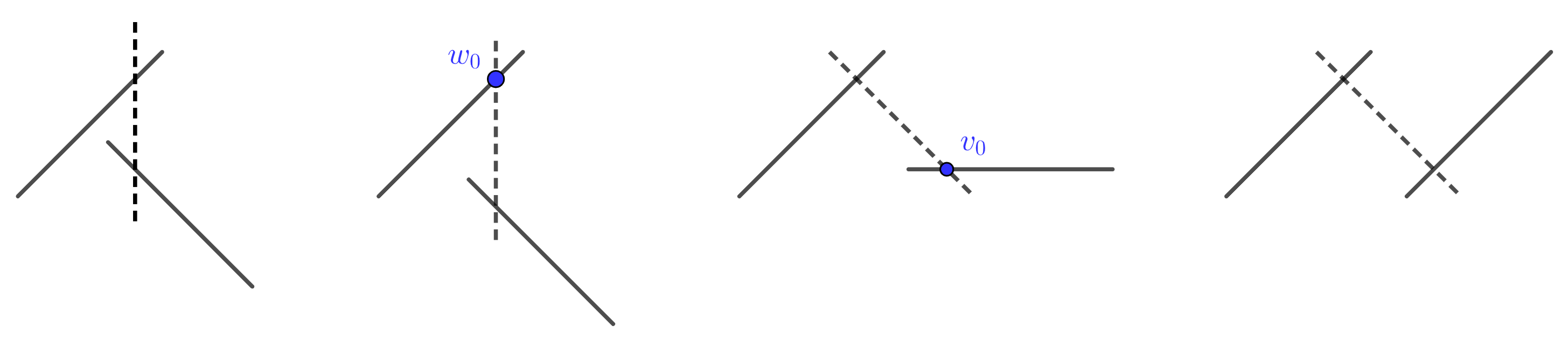
Figure 9. The projections on the $xy$-plane of the images of core curves $\Sigma^{g}_{k+1,N}$, $\Sigma^{g}_{k+1,N+1}$, $\Sigma^{g}_{k+1,N+2}$ under identity, $H^{(1)}_{1}$, $H^{(2)}_{1}\circ H^{(1)}_{1}$, and $H^{(3)}_{1}\circ H^{(2)}_{1}\circ H^{(1)}_{1}$.

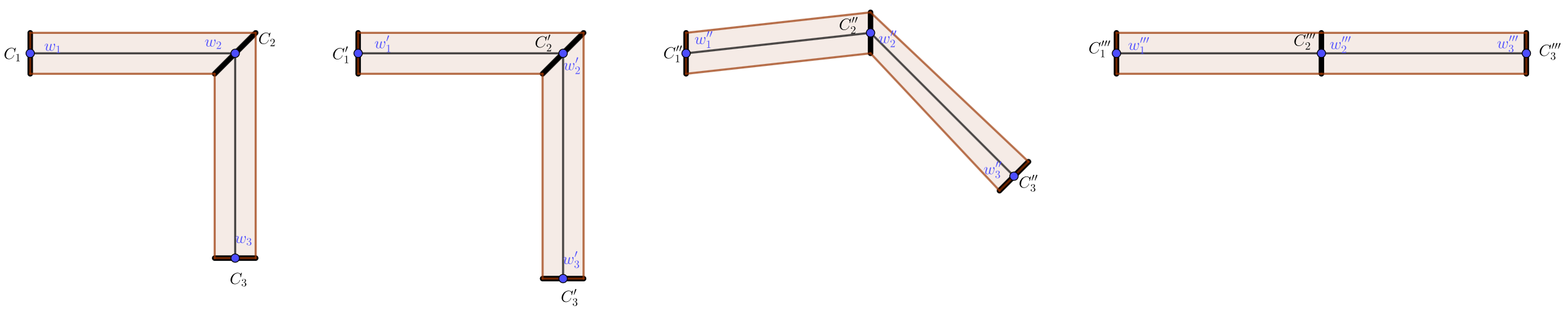
Figure 10. The projections on the $xy$-plane of $S_{4}$ (first figure), $S_{4}^{\prime}$ (second figure), $S_{4}^{\prime\prime}$ (third figure), $H^{(3)}(S_{4}^{\prime\prime})$ (fourth figure).

For the second step, set $S_{i}^{\prime}=H^{(1)}_{1}(S_{i})$ for $i=1,2,3,4$, set $w_{i}^{\prime}=H^{(1)}_{1}(w_{i})$ for $i=1,2,3$, and set $C_{i}^{\prime}=H^{(1)}_{1}(C_{i})$ for $i=1,2,3$. We define one more auxiliary point. Let $\pi:\mathbb{R}^{3}\to\{z=0\}$ be the projection on the $xy$-plane and let $w_{0}$ be the unique point in the intersection $\pi(S_{1}^{\prime})\cap\pi(S_{2}^{\prime})$.

Let $R_{t}$ be the counterclockwise rotation map by $t\pi/4$ with respect to the line $\pi^{-1}(\{w_{0}\})$. We also use a bi-Lipschitz deformation that takes an ellipse to a circle of the same center as the ellipse and radius equal to the semi-minor axis. In particular if $a\in(0,1)$ and $r>0$,

(A.1) $$(r\cos{\theta},ar\sin{\theta})\mapsto((r+rat-rt)\cos{\theta},ar\sin{\theta}),\qquad\text{$\theta\in[0,2\pi]$ and $t\in[0,1]$}.$$

Define now a bi-Lipschitz deformation $H^{(2)}=\{H^{(2)}_{t}:H^{(1)}_{1}(\partial V_{2})\to\mathbb{R}^{3}\}_{t\in[0,1]}$ such that

• $H^{(2)}_{t}|S_{1}^{\prime}$ is the identity,

• $H^{(2)}_{t}|S_{2}^{\prime}\cup S_{3}^{\prime}=R_{t}$,

• $H^{(2)}_{t}|C_{2}^{\prime}$ is the composition of $R_{t}$ and an “ellipse-to-circle” deformation as in (A.1),

• $H^{(2)}_{t}|S_{4}^{\prime}$ is a linear interpolation of the maps $H^{(2)}_{t}|C_{1}^{\prime}$, $H^{(2)}_{t}|C_{2}^{\prime}$, and $H^{(2)}_{t}|C_{3}^{\prime}$.

For the third and final step, set $S_{i}^{\prime\prime}=H^{(2)}_{1}(S_{i}^{\prime})$ for $i=1,2,3,4$, set $w_{i}^{\prime\prime}=H^{(2)}_{1}(w_{i}^{\prime})$ for $i=1,2,3$, and set $C_{i}^{\prime\prime}=H^{(2)}_{1}(C_{i}^{\prime})$ for $i=1,2,3$. We define one more auxiliary point. Let $v_{0}$ be the unique point in the intersection $\pi(S_{2}^{\prime\prime})\cap\pi(S_{3}^{\prime\prime})$.

Let $R_{t}^{\prime}$ be the counterclockwise rotation by $t\pi/4$ with respect to the line $\pi^{-1}\{v_{0}\}$. Define now a bi-Lipschitz deformation $H^{(3)}=\{H^{(2)}_{t}:H^{(2)}_{1}(H^{(1)}_{1}(\partial V_{2}))\to\mathbb{R}^{3}\}_{t\in[0,1]}$ such that

• $H^{(3)}_{t}|S_{1}^{\prime\prime}\cup S_{2}^{\prime\prime}$ is the identity,

• $H^{(3)}_{t}|S_{3}^{\prime\prime}=R_{t}^{\prime}$,

• $H^{(3)}_{t}|C_{2}^{\prime\prime}$ is a translation with $H^{(3)}_{t}(C_{2}^{\prime\prime})$ being centered at $R_{t}^{\prime}(w_{2}^{\prime\prime})$,

• $H^{(3)}_{t}|S_{4}^{\prime\prime}$ is a linear interpolation of the maps $H^{(3)}_{t}|C_{1}^{\prime\prime}$, $H^{(3)}_{t}|C_{2}^{\prime\prime}$, and $H^{(3)}_{t}|C_{3}^{\prime\prime}$.

We finish by concatenating the deformations $H^{(1)},H^{(2)},H^{(3)}$ and obtain $H$ by defining $H_{t}=H^{(1)}_{3t}$ if $t\in[0,1/3]$, $H_{t}=H^{(2)}_{3t-1}$ if $t\in[1/3,2/3]$, and $H_{t}=H^{(3)}_{3t-2}$ if $t\in[2/3,1]$. ∎

Appendix B UQR power maps

It is well-known that there exist UQR analogues of power mappings in $\overline{\mathbb{R}^{3}}$ of degree $d^{2}$, where $d\geq 2$. These were first constructed by Mayer [May97]. It is perhaps less well-known that other degrees may be achieved.

Proposition B.1.

There exists a UQR map $f:\overline{\mathbb{R}^{3}}\to\overline{\mathbb{R}^{3}}$ of degree $2$ with Julia set equal to $S^{2}$.

Proof.

If $x=(x_{1},x_{2},x_{3})\in\mathbb{R}^{3}$, let $G$ be the discrete group of isometries in $\mathbb{R}^{3}$ generated by $g_{1}(x)=x+(1,0,0)$, $g_{2}(x)=x+(0,1,0)$ and $g_{3}$ the rotation about the $x_{3}$-axis by angle $\pi$. Then there is a Zorich map $\mathcal{Z}$ which is strongly automorphic with respect to $G$ and which maps the plane $\{x_{3}=0\}$ onto the unit sphere $S^{2}$ (see, for example, [FM20] for more details on this).

Let $A$ be the linear map which is a composition of a dilation with scaling factor $\sqrt{2}$ and a rotation by $\pi/4$ about the $x_{3}$-axis, that is,

$$A(x_{1},x_{2},x_{3})=(x_{1}-x_{2},x_{1}+x_{2},\sqrt{2}x_{3}).$$

We need $AGA^{-1}\subset G$ and it is sufficient to check that this is so on the generators. Clearly $Ag_{3}A^{-1}=g_{3}$. Next, by the linearity of $A$, we have

$$Ag_{1}A^{-1}(x)=A\left(A^{-1}(x)+(1,0,0)\right)=x+A(1,0,0)=x+(1,1,0)=g_{2}(g_{1}(x))$$

and hence $Ag_{1}A^{-1}\in G$. Finally,

$$Ag_{2}A^{-1}(x)=A\left(A^{-1}(x)+(0,1,0)\right)=x+A(0,1,0)=x+(-1,1,0)=g_{2}(g_{1}^{-1}(x))$$

and hence $Ag_{2}A^{-1}\in G$. Thus by, for example, [FM20, Theorem 3.4] we conclude that there is a UQR map $f:\mathbb{R}^{3}\to\mathbb{R}^{3}$ which solves the Schröder equation $f\circ\mathcal{Z}=\mathcal{Z}\circ A$. Proceeding as Mayer [May97], we see that $f$ extends over the point at infinity, the Julia set of $f$ is $\mathbb{S}^{2}$, and $f$ has degree $2$. ∎

We may use the map from Proposition B.1 to prove Theorem 5.3.

Proof of Theorem 5.3.

Let $f$ be the UQR map of degree $2$ from Proposition B.1, and denote by $P_{d}$, for $d\geq 2$, the UQR power maps constructed by Mayer [May97] using the Zorich map $\mathcal{Z}$ above. Then following the argument in [Fle19, §5.1], $\mathcal{F}$ is a quasiregular semigroup, where $\mathcal{F}$ is generated by $f$ and the collection of $P_{d}$’s with Julia set $J(\mathcal{F})=\mathbb{S}^{2}$. In particular, the map $f^{n}\circ P_{d}$ is UQR with the required properties. ∎

References

- [Arm66] Steve Armentrout, Decompostions of with a compact -dimensional set of nondegenerate elements, Trans. Amer. Math. Soc. 123 (1966), 165–177. MR 195074
- [BE79] Israel Berstein and Allan L. Edmonds, On the construction of branched coverings of low-dimensional manifolds, Trans. Amer. Math. Soc. 247 (1979), 87–124. MR 517687
- [Fle19] Alastair N. Fletcher, Quasiregular semigroups with examples, Disc. Cont. Dyn. Syst. 39 (2019), no. 4, 483–520. MR 4179769
- [FM20] Alastair N. Fletcher and Doug Macclure, Strongly automorphic mappings and julia sets of uniformly quasiregular mappings, J. Anal. Math. 141 (2020), 2157–2172. MR 3927507
- [FN11] Alastair N. Fletcher and Daniel A. Nicks, Julia sets of uniformly quasiregular mappings are uniformly perfect, Math. Proc. Cam. Phil. Soc. 151 (2011), no. 3, 541–550. MR 2838349
- [FS21] Alastair Fletcher and Daniel Stoertz, Spiders’ webs of doughnuts, Rev. Mat. Iberoam. 37 (2021), no. 1, 161–176. MR 4201409
- [FS22] Alastair Fletcher and Daniel Stoertz, Genus 2 Cantor sets, arXiv preprint (2022).
- [FV21] Alastair Fletcher and Vyron Vellis, On uniformly disconnected julia sets, Math. Z. 299 (2021), 853–866. MR 4311621
- [FW15] Alastair Fletcher and Jang-Mei Wu, Julia sets and wild Cantor sets, Geom. Dedicata 174 (2015), 169–176. MR 3303046
- [HR02] Juha Heinonen and Seppo Rickman, Geometric branched covers between generalized manifolds, Duke Math. J. 113 (2002), no. 3, 465–529. MR 1909607
- [IM96] Tadeusz Iwaniec and Gaven Martin, Quasiregular semigroups, Ann. Acad. Sci. Fenn. Math. 21 (1996), no. 2, 241–254. MR 1404085
- [May97] Volker Mayer, Uniformly quasiregular mappings of Lattès type, Conform. Geom. Dyn. 1 (1997), 104–111. MR 1482944
- [Moi77] Edwin E. Moise, Geometric topology in dimensions and , Graduate Texts in Mathematics, Vol. 47, Springer-Verlag, New York-Heidelberg, 1977. MR 0488059
- [Mun66] James R. Munkres, Elementary differential topology, revised ed., Annals of Mathematics Studies, No. 54, Princeton University Press, Princeton, N.J., 1966, Lectures given at Massachusetts Institute of Technology, Fall, 1961. MR 0198479
- [PRW14] Pekka Pankka, Kai Rajala, and Jang-Mei Wu, Quasiregular ellipticity of open and generalized manifolds, Comput. Methods Funct. Theory 14 (2014), no. 2-3, 383–398. MR 3265368
- [Ric93] Seppo Rickman, Quasiregular mappings, Ergebnisse der Mathematik und ihrer Grenzgebiete (3) [Results in Mathematics and Related Areas (3)], vol. 26, Springer-Verlag, Berlin, 1993. MR 1238941
- [TV81] P. Tukia and J. Väisälä, Lipschitz and quasiconformal approximation and extension, Ann. Acad. Sci. Fenn. Ser. A I Math. 6 (1981), no. 2, 303–342 (1982). MR 658932
- [V8̈6] Jussi Väisälä, Bi-Lipschitz and quasisymmetric extension properties, Ann. Acad. Sci. Fenn. Ser. A I Math. 11 (1986), no. 2, 239–274. MR 853960
- [Ž05] Matjaž Željko, Genus of a Cantor set, Rocky Mountain J. Math. 35 (2005), no. 1, 349–366. MR 2117612