Regularized Graph Structure Learning with Semantic Knowledge
for Multi-variates Time-Series Forecasting

Abstract

Multivariate time-series forecasting is a critical task for many applications, and graph time-series network is widely studied due to its capability to capture the spatial-temporal correlation simultaneously. However, most existing works focus more on learning with the explicit prior graph structure, while ignoring potential information from the implicit graph structure, yielding incomplete structure modeling. Some recent works attempts to learn the intrinsic or implicit graph structure directly, while lacking a way to combine explicit prior structure with implicit structure together. In this paper, we propose Regularized Graph Structure Learning (RGSL) model to incorporate both explicit prior structure and implicit structure together, and learn the forecasting deep networks along with the graph structure. RGSL consists of two innovative modules. First, we derive an implicit dense similarity matrix through node embedding, and learn the sparse graph structure using the Regularized Graph Generation (RGG) based on the Gumbel Softmax trick. Second, we propose a Laplacian Matrix Mixed-up Module (LM³) to fuse the explicit graph and implicit graph together. We conduct experiments on three real-word datasets. Results show that the proposed RGSL model outperforms existing graph forecasting algorithms with a notable margin, while learning meaningful graph structure simultaneously. Our code and models are made publicly available at https://github.com/alipay/RGSL.git.

1 Introduction

The spatial-temporal graph network Yu et al. (2018); Cao et al. (2020); Chen et al. (2019); Shang et al. (2021) enhances time-series forecasting by modelling the correlation as well as the relationship between multivariate time-series. It has many applications. For example, the traffic flow forecasting is a basic yet important application in intelligent transportation system, which constructs the spatial dependency graph with road distance. The cloud service flow forecasting is a fundamental task in cloud serving system and e-commerce domain, which builds the relationship graph based on request region or zone information. Existing graph time-series forecasting networks like STGCN Yu et al. (2018), DCRNN Li et al. (2018) and ASTGCN Guo et al. (2019) exploit fixed graph structure constructed with domain expert knowledge to capture the multi-variate time-series relationship. The explicit graph is not always available in every applications or may be incomplete as it is hard for human expert to capture latent or long-range dependence among substantial time-series. Thus how to define accurate dynamic relationship graph becomes a critical task for graph time-series forecasting.

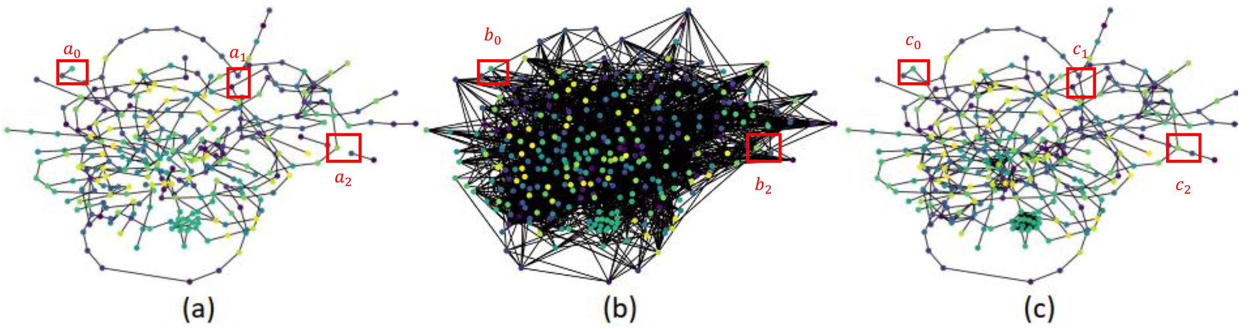
Figure 1: Graph Visualization (a) naive explicit GSL trained from prior knowledge; (b) implicit GSL from popular network AGCRN; (c) our proposed RGSL

As the quality of graph structure impacts the performances of graph time-series forecasting greatly, many recent efforts  Lu et al. (2021); Bai et al. (2020); Chen et al. (2021a) have made for Graph Structure Learning (GSL). For instance, GTS  Shang et al. (2021) have been proposed to learn the discrete graph structure simultaneously with GNN. AGCRN in  Bai et al. (2020) is proposed to learn the similarity matrix derived from trainable adaptive node embedding and forecasting in an end-to-end style. DGNN  Lu et al. (2021) is a dynamic graph construction method which learns the time-specific spatial adjacency matrix firstly and then exploits dynamic graph convolution to pass the message. However, these aforementioned methods go to another extreme that they learn the intrinsic/implicit graph structure from time-series patterns directly, while ignoring the possibility to leverage priori time-series relationships defined from domain expert knowledge.

In this paper, we focus on solving two problems, the first is how to take advantage of combining the explicit time-series relationship with implicit correlations effectively in an end-to-end way; the second is how to regularize the learned graph to be sparse which filters out the redundant useless edges thus improves overall performances, and is more valuable to real-world applications. To address these issues, firstly we introduce the Regularized Graph Generation (RGG) module to learn the implicit graph, which adopts the Gumbel Softmax trick to sparsify the dense similarity matrix from node embedding. Second, we introduce the Laplacian Matrix Mixed-up Module (LM³) to incorporate the explicit relationship from domain knowledge with the implicit graph from RGG. Figure1 shows the graph structure learned from only explicit relationship in (a), both implicit and explicit relationship without regularization (b), as well as from our proposed RGSL shown in (c). We can observe that RGSL can discover the implicit time-series relationship ignored by naive graph structure learning algorithm(shown in red boxes in Figure1(a)). Besides, compared to Figure 1(b), the regularization module in RGSL which automatically removes the noisy/redundant edges making the learned graph more sparse, as well as more effective than dense graph.

To summarize, our work presents the following contributions.

• We propose a novel and efficient model named RGSL which first exploits both explicit and implicit time-series relationship to assist graph structure learning, and our proposed LM³ module effectively mixes up two kinds of Laplacian matrix collectively.

• Besides, to regularize the learned matrix, we also propose a RGG module which formulates the discrete graph structure as a variable independent matrix and exploits the Gumbel softmax trick to optimize the probabilistic graph distribution parameters.

• Extensive experiments show the proposed model RGSL significantly outperforms benchmarks on three datasets consistently. Moreover, both the LM³ module and RGG module can be easily generalized to different spatio-temporal graph models.

2 Methodology

In this section, we first introduce problem definition and notations, and then describe the detailed implementation of proposed RGSL. The overall pipeline is shown in Figure 2. The RGSL consists of three major modules, and the first is the regularized graph generation module name RGG which learns the discrete graph structure with trainable node embeddings in Section 2.2 with Gumbel softmax trick. The second is the Laplacian matrix mix-up module named LM³ in 2.3 which captures both explicit and implicit time-series correlations between nodes in a convex way. Finally, in 2.4, we utilize recurrent graph network to perform time-series forecasting considering both the spatial correlation and temporal dependency simultaneously.

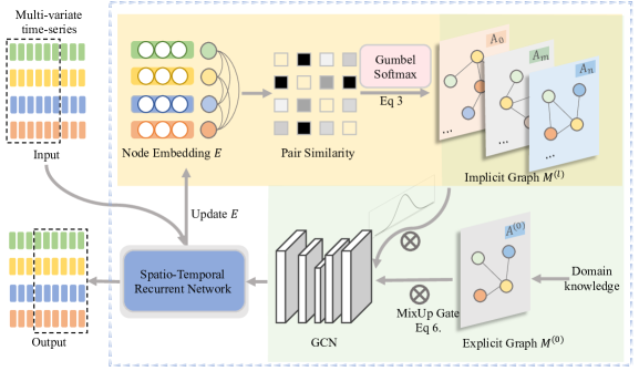
Figure 2: The framework of RGSL: it consists of three modules. Regularized Graph Generation(RGG) module (inside the yellow box) takes trainable node embedding $\bm{E}$ as input and outputs learned discrete graph $\bm{A^{(l)}}$; then Laplacian Matrix Mix-up Module(LM³) (inside the green box) outputs adjacent matrix $\bm{A}$ which encodes both explicit knowledge $\bm{M^{(0)}}$ and implicit knowledge $\bm{M^{(l)}}$. $\bm{A}$ goes through spatial-temporal graph convolution recurrent network(inside the blue dashed box) to give the forecasting results.

2.1 Preliminary

The traffic series forecasting is to predict the future time series from historical traffic records. Denote the training data by $\bm{{X_{0:T}}}=\{\bm{X_{0}},\bm{X_{1}},\ldots,\bm{X_{t}},\ldots,\bm{X_{T}}\}$, and $\bm{X_{t}}=\{\bm{X_{t}^{0}},\bm{X_{t}^{1}},\ldots,\bm{X_{t}^{N}}\}$, where the superscript refers to series and subscript refers to time. There are total T timestamps for training and $\bm{\tau}$ timestamps required for traffic forecasting. We denote $\bm{\mathcal{G}^{(0)}}$ as the explicit graph constructed with priori time-series relationship, and $\bm{\mathcal{G}^{(l)}}$ as the implicit graph learned from trainable node embeddings, and the vertex of graph $\bm{\mathcal{G}^{(l)}}$ represents traffic series $\bm{\mathcal{X}}$, and $\bm{A}\in\mathbb{R}^{N\times N}$ is the adjacent matrix of the graph $\bm{\mathcal{G}}$ representing the similarity between time-series. Thus, the time-series forecasting with the explicit graph task can be defined as:

$$\small\min_{W_{\theta}}\bm{\mathcal{L}}(\bm{X}_{T+1:T+\tau},\bm{\hat{X}}_{T+1:T+\tau};\bm{X}_{0:T},\bm{\mathcal{G}}^{(0)},\bm{\mathcal{G}}^{(l)})$$ (1)

where ${W_{\theta}}$ denotes all the learnable parameters, $\bm{\hat{X}}_{T+1:T+\tau}$ denotes the ground truth future values, $\bm{\mathcal{L}}$ is the loss function.

2.2 Regularized Graph Generation

Regularization method Dropout Srivastava et al. (2014) aims at preventing neural networks from overfitting by randomly drop connections during training. However, traditional Dropout equally treats every connection and drop them with the same distribution acquired from cross-validation, which doesn’t consider the different significance of different edges. In our Regularized Graph Generation(RGG) module, inspired by Shang et al. (2021) and works in reinforcement learning, we simply resolve the regularization problem with Gumble Softmax to replace Softmax, which is super convenient to employ, increases the explainability of prediction and shows nice improvements. Another motivation of applying Gumble Softmax trick is to alleviate the density of the learned matrix after training from GNNs.

Let $\bm{E}\in\mathbb{R}^{N\times d}$ be the learned node embedding matrix, $d$ is the embedding dimension, $\bm{\theta}$ is the probability matrix then $\bm{\theta}_{ij}\in\bm{\theta}$ represents the probability to preserve the edge of time-series $i$ to $j$, which is formulated as:

$$\small\bm{\theta}=\bm{E}\bm{E}^{\top}$$ (2)

Let $\sigma$ be activation function and $s$ is the temperature variable, then the sparse adjacency matrix $\bm{A}^{(l)}$ is defined as:

$$\bm{A}^{(l)}= \sigma((\log(\bm{\theta}_{ij}/(1-\bm{\theta}_{ij}))+(g_{ij}^{1}-g_{ij}^{2}))/s)$$ (3)

$$s.t.\quad g_{ij}^{1},g_{ij}^{2}\sim Gumbel(0,1)$$

Equation 3 is the Gumbel softmax implementation of our task where the $\bm{A}^{(l)}_{ij}=1$ with the probability $\bm{\theta}_{ij}$ and 0 with remaining probability. It can be easily proved that Gumbel Softmax shares the same probability distribution as the normal Softmax, which ensures that the graph forecasting network keeps consistent with the trainable probability matrix generation statistically.

At each iteration, we calculate the adjacent matrix $\bm{\theta}$ as the Equation 2 suggests, Gumbel-Max samples the adjacent matrix to determine which edge to preserve and which to discard, which is similar to Dropout. However, dropout randomly selects edges or neurons with equal probability, while we drop out useful edges with small likelihood and tend to get rid of those redundant edges. As in Figure. 4(a), all the non-diagonal entries are non-zero, but substantial amounts of them are small-value and regarded as useless or even noisy. Another difference from dropout is that in test phase, RGG also utilizes Gumbel Softmax to remove the noise information contained in redundant small values. In this way, we filter out the similarity information between nodes which is beneficial for later traffic predicting, and also inherit the advantages of dropout such as improving the regularization and generalization, and preventing too much co-adapting. From another perspective, RGG also improves the explainability in graph time-series prediction since $\bm{A}^{(l)}$ is sparse which is more similar to semantic knowledge shown in Figure. 1.

The RGG module regularizes the learnable graph generated with trainable node embeddings, making it more explainable. It is easy to add to graph generation tasks, significantly reducing the computation cost.

2.3 Laplacian Matrix Mix-up Module

There are many kinds of attributes in time-series, for example in traffic time-series forecasting task, each node $\bm{X_{0:T}^{i}}$ represents flows in a POI, whose properties are affected by multiple complicated factors: location, time of the day, nearby commercial buildings, and so on. We classify the factors into three categories: 1) temporal dependencies; 2) spatial dependencies; 3) external factors. The first two factors are easy to understand, and external factors can be illustrated in this example: although road A and road B are not connected spatially, they are both six-lane avenues and have gas stations on them, thus we assume A and B may share similar patterns. We propose a Laplacian matrix mix-up module named LM³ which carefully fuses both the explicit graph generated from priori relationship and the implicit graph calculated with trainable node embeddings, discovering the above three categories of relationship.

The spatial adjacent information is often provided with datasets themselves, or can be acquired with little effort from urban maps. Let’s denote them as explicit graph $\bm{A}^{(0)}$, then the spatially adjacent relationship is easily captured by$\{{\mathbf{X}_{0:T}}^{j}\},\ s.t.\ \bm{A}_{i,j}^{(0)}=1$. Although the explicit graph may not include complete information, it contains spatial correlations and can be set as the training start-point. On the other hand, the $\bm{A}^{(l)}$, derived from Eq.3, encodes the inner product of node embeddings, and captures the implicit correlation between multivariate time-series. Let $\bm{X}\in\mathbb{R}^{N\times H}$ be input matrix, $\bm{W}^{(0)}$, $\bm{W}_{b}^{(0)}$, $\bm{W}^{(l)}$, $\bm{W}_{b}^{(l)}$ are learnable parameters, then the Chebyshev polynomial expansion form of graph operations for $\bm{A}^{(l)}$ (Eq.5) and $\bm{A}^{(0)}$ (Eq.4)

$$\bm{\tilde{A}}^{(0)}(\bm{X})=(\bm{I}+\bm{D}^{-\frac{1}{2}}\bm{A}^{(0)}\bm{D}^{-\frac{1}{2}})\bm{X}\bm{W}^{(0)}+\bm{W}_{b}^{(0)}$$ (4)

$$\bm{\tilde{A}}^{(l)}(\bm{X})=(\bm{I}+\bm{D}^{-\frac{1}{2}}\bm{A}^{(l)}\bm{D}^{-\frac{1}{2}})\bm{X}\bm{W}^{(l)}+\bm{W}_{b}^{(l)}$$ (5)

where $\bm{I}\in\mathbb{R}^{N\times N}$, $\bm{D}$ is the degree matrix.

The mix-up operation originally serves as a data augmentation method to better constrain the border of the feature space, and we apply the idea of ’mix-up’ here to balance the composition of two kinds of correlations, and constrain the border of Adjacent Matrix.

Besides, different from traditional mix-up which samples weighting coefficients from beta distribution, we compute the weights by self-attention module, which dynamically assigns higher weights to the high intra-similarity between long-distance nodes, and further improves mining the semantic correlations. As the following equation suggests, LM³ mixes up the explicit graph $\bm{A}^{(0)}$ with learned implicit graph $\bm{A}^{(l)}$ in a convex dynamic manner.

$$\small\bm{M}^{(m)}(\bm{X})=f_{a}(\tilde{\bm{A}}^{(0)}(\bm{X});\bm{\theta}_{a})+f_{a}(\tilde{\bm{A}}^{(l)}(\bm{X});\bm{\theta}_{a})$$ (6)

where $f_{a}$ denotes self-attention network, $\bm{\theta}_{a}$ and $\bm{\theta}_{b}$ are the parameters of attention network. By utilizing LM³ module, the dynamic convex combination of explicit graph and learned implicit graph, we carefully capture the two kinds of time-series correlation. And the experiments can demonstrate our assumption in Section 3.4.

2.4 Spatial Temporal Recurrent Convolution Network

As illustrated in Figure2, we first take the learnable nodes embedding $\bm{E}$ as inputs Eq.3 and output the probability graph $\bm{A}^{(l)}$. Then, we apply the Chebyshev polynomial expansion form of graph operations for both $\bm{A}^{(l)}$ and $\bm{A}^{(0)}$ and put the encoding graph into LM³ module Eq.6 to get $\bm{M}^{(m)}$. In order to further understand the spatial and temporal inter-dependencies between traffic series, our method takes $\bm{X}_{0:T}$ and $\bm{M}^{(m)}$ as input, then put it to Spatial Temporal Recurrent Graph Convolution Module (STRGC) which contains a graph convolution network and a Gate Recurrent Unit (GRU) network to updates hidden states $\bm{h}_{t}$ collectively as the equations 7. It is worth noting that many sequence and graph architectures can be applied here, we opt for a simple but effective one to model the dynamic and comprehensive spatial-temporal correlations, and finally outputs time series predictions $\bm{X}_{T+1:T+\tau}$.

$$\bm{z}_{t}=\sigma(\bm{M}^{(m)}([\bm{X}_{0:t},\bm{h}_{t-1}]))$$ (7)

$$\bm{r}_{t}=\sigma(\bm{M}^{(m)}([\bm{X}_{0:t},\bm{h}_{t-1}]))$$

$$\bm{\hat{h}}_{t}=tanh(\bm{M}^{(m)}([\bm{r}_{t}\odot\bm{h}_{t-1},\bm{X}_{0:t}]))$$

$$\bm{h}_{t}=\bm{z}_{t}\odot\bm{h}_{t-1}+(1-\bm{z}_{t})\odot\bm{\hat{h}}_{t}$$

where the embedded graph information is sent into reset gate $\bm{r}_{t}$ and update gate $\bm{z}_{t}$, and $\sigma$ refers to sigmoid function.

$$\small\mathcal{L}(\bm{W}_{\theta})=\frac{1}{\tau}|{\bm{X}_{T+1:T+\tau}}-\bm{\hat{X}}_{T+1:T+\tau}|$$ (8)

The loss function in our method is mean absolute error (MAE) loss formulated as Eq. 8.

Table 1: Overall prediction performance of different methods on the PeMSD4 and PeMSD8 dataset, and results in boldface are the best performance achieved. (smaller value means better performance)

	Methods	PeMSD4 Dataset			PeMSD8 Dataset
		MAE $\bm{\downarrow}$	RMSE $\bm{\downarrow}$	MAPE $\bm{\downarrow}$	MAE $\bm{\downarrow}$	RMSE $\bm{\downarrow}$	MAPE $\bm{\downarrow}$
Sequence	HA	38.03	59.24	27.88%	34.86	52.04	24.07%
	ARIMA	36.84	55.18	-	34.27	48.88	-
	VAR	24.54	38.61	17.24%	19.19	29.81	13.10%
	SVR	24.44	37.76	17.27%	20.92	31.23	14.24%
	GRU-ED	23.68	39.27	16.44%	22.00	36.23	13.33%
	FC-LSTM  Sutskever et al. (2014)	23.60	37.11	16.17%	21.28	31.88	13.72%
	DSANet  Huang et al. (2019)	22.79	35.77	16.03%	17.14	26.96	11.32%
Graph	DCRNN Li et al. (2018)	21.22	33.44	14.17%	16.82	26.36	10.92%
	STGCN  Yu et al. (2018)	21.16	34.89	13.83%	17.50	27.09	11.29%
	ASTGCN  Guo et al. (2019)	22.93	35.22	16.56%	18.25	28.06	11.64%
	STSGCN  Song et al. (2020b)	21.19	33.65	13.90%	17.13	26.86	10.96%
	AGCRN Bai et al. (2020)	19.83	32.26	12.97%	15.95	25.22	10.09%
	Z-GCNETs Chen et al. (2021b)	19.54	31.33	12.87%	16.12	25.74	10.35%
	Ours	19.19	31.14	12.69%	15.49	24.80	9.96%
	Improvements	+1.79%	+0.61%	+1.40%	+3.91%	+3.65%	+3.92%

3 Experiments

3.1 Datasets

To evaluate the performance of the proposed RGSL, we conduct experiments on two public real-world traffic datasets PeMSD4 and PeMSD8  Guo et al. (2019); Song et al. (2020a), and a proprietary dataset RPCM.
PeMSD4: The PeMSD4 dataset refers to the traffic flow data in the San Francisco Bay Area and contains 3848 detectors on 29 roads. The time span of this dataset is from January to February in 2018
PeMSD8: The PeMSD8 dataset contains traffic flow information collected from 1979 detectors on 8 roads on the San Bernardino area from 1/Jul/2016 - 31/Aug/2016.
RPCM: The RPCM dataset collects Remote Procedure Call(RPC) data every ten minutes provided by a world leading internet company. The RPC data is a direct reflection of the remote communications and mutual calls between distributed systems. RPCM contains time series from 113 applications deployed in different Logic Data Center(LDC).

3.2 Baselines

To evaluate the overall performance of our work, we compare our model RGSL with traditional methods and deep models as follows.

1) Sequence models which classically focus on capturing temporal relations among series, such as Historical Average (HA) which uses the average of the same historical timestamps as predictions, Vector Auto-Regression (VAR)  Zivot and Wang (2006), support vector regression (SVR) Drucker et al. (1997), Auto-Regressive Integrated Moving Average (ARIMA)  Williams and Hoel (2003) which is a statistics method modelling time dependencies; GRU-ED which is GRU-based encoder-decoder framework; FC-LSTM Sutskever et al. (2014) uses long short-term memory (LSTM) and encoder decoder network;Dual Self-attention Network(DSANet)  Huang et al. (2019) using CNN and self-attention mechanism for temporal and spatial correlations respectively;

2) Deep graph models: Diffusion convolutional recurrent neural network(DCRNN)  Li et al. (2018) which adopts a diffusion process on a directed graph to model the traffic flow, utilizes bidirectional random walks, and combines GCN with recurrent models in an encoder-decoder manner; Spatio-temporal graph convolutional network(STGCN)  Yu et al. (2018) exploits spatial convolution and temporal convolution for forecasting; Attention-based spatio-temporal graph convolutional network(ASTGCN)  Guo et al. (2019) which integrates attention mechanisms based on STGCN for capturing dynamic spatial and temporal patterns; Spatial-Temporal Synchronous Graph Convolutional Network(STSGCN)  Song et al. (2020a) which addresses heterogeneities in spatial-temporal data and designs multiple modules for different time periods; Adaptive Graph Convolutional Recurrent Network (AGCRN)  Bai et al. (2020) which learns node-specific and data-adaptive graph to capture fine-grained features; GCNs with a time-aware zigzag topological layer (Z-GCNETs) Chen et al. (2021b) introduces the concept of zigzag persistence into time-aware GCN.

Evaluation Metrics: In this paper, we use mean absolute error (MAE), mean absolute percentage error (MAPE), and root-mean-square error (RMSE) to measure the performance.

3.3 Results

Table 2: Component-wise analysis. Ablation study on explicit graph and implicit graph which are inputs of LM³, as well as RGG and LM³.

#	Explicit	Implicit	$LM^{3}$	RGG	RPCM Dataset			PeMSD4 Dataset
	Graph	Graph	Module	Module	MAE $\bm{\downarrow}$	RMSE $\bm{\downarrow}$	MAPE $\bm{\downarrow}$	MAE $\bm{\downarrow}$	RMSE $\bm{\downarrow}$	MAPE $\bm{\downarrow}$
1	✓				$0.05$	$0.08$	$60.13\%$	$25.13$	$38.82$	$17.62\%$
2		✓			$0.04$	$0.06$	$32.86\%$	$19.84$	$32.35$	$13.01\%$
3	✓	✓			$0.03$	$0.06$	$30.54\%$	$19.47$	$31.85$	$12.85\%$
4	✓	✓	✓		$0.03$	$0.06$	$27.86\%$	$19.37$	$31.50$	$12.82\%$
5	✓	✓	✓	✓	0.03	0.05	$\textbf{24.77}\%$	19.19	31.14	$\textbf{12.69}\%$

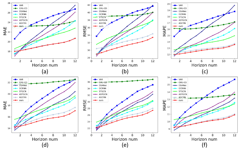
Figure 3: Evaluation metrics at each horizon in prediction period on PeMSD4 (a,b,c) and PeMSD8 (d,e,f) dataset

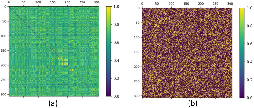
Figure 4: RGG effect on adjacent matrix; (a) are adjacent matrix after Softmax; (b)are adjacent matrix after GumbleSoftmax;

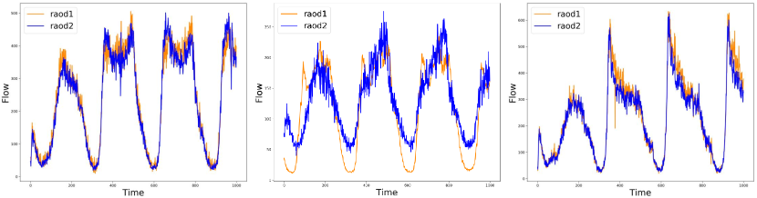
Figure 5: RGSL is able to excavate implicit relationships (road 1 and road 2). Road 1 and road2 share similar peaks and valleys, trends and timestamps.

The overall experimental results, including our RGSL and other baselines are shown in Table 1. We summarize the results in the following three aspects: 1) GCN-based deep methods outperform other methods, which is reasonable since graph pays more attention to spatial correlations; 2) Our method further improves traffic forecasting methods with a significant margin at all metrics. Our RGSL outperforms AGCRN by 3.22% MAE on PeMSD4 and around 2.88% MAE on PeMSD8 mainly result from 2 reasons. The first is that AGCRN totally ignores the explicit graph knowledge. Secondly, AGCRN learns dense and somehow redundant adjacent matrix. We demonstrate the above explanations after add on our module, as shown in table 3. Z-GCNETs performs better than AGCRN (relatively 1% in MAE and MAPE, but inferior about 1% in RMSE). And one of the differences is Z-GCNETs utilizes explicit graph information, demonstrating the significance of prior knowledge. Z-GCNETs processes raw data in part, regards each part as a channel and stacks channel-wise layers, which can capture more detailed features, but it also has graph redundancy problem. 3) The proposed method significantly outperforms other methods by 0.61% - 3.92% relative improvements corroborates that regularization plays an important role in graph networks, and carefully collaborating prior knowledge and learned correlations is promising and worthwhile. Experiments results in Figure5 shows that road 1 and road 2 are not spatially connected and thus not existed in prior explicit graph, but RGSL captures their similarity and is able to model this similarity by learning $A^{(l)}$. Besides, in Figure3our model also shows superior for all horizons and deteriorate slower than other GCN-based models.

3.4 Ablation Study

Table2 illustrates the effect of removing key components of our method on both PeMSD4 and RPCM dataset. There are two main modules LM³ and RGG, and LM³ takes prior graph and learnable graph as input.

Table2 shows four ablations that removing RGG module results in degradation(relative 1%) due to the lack of regularization. Besides, removing RGG also makes adjacent matrix less explainable, as in Figure4(b), the learned adjacent matrix is filled with small enties. 4(b) and 1(c) are adjacent matrix with LM³ module, it is sparse and accord with our expectation.

Table2 experiment 3,2,1 and Figure 1 shows the effect of LM³ module, while experiment 1 and 2 respectively takes prior knowledge or learned knowledge as the only graph input. The substantial decrease in performance demonstrates the followings: 1)only the explicit graph restricts the sum of learnable parameters and lacks flexibility; 2) learnable-only graph performs far better than priori graph, yet miss plenty of useful knowledge. As shown in 1(a), compared to (c), it lacks some key edges(in red boxes); 3) utilizing both prior and learnable knowledge by simply add them up shows small gain in performances, but is inferior to our carefully designed convex dynamic pattern, since the fixed parameters lacks the ability to weight the importance of the above two matrix according to their distributions. Overall, our modules shows great potential to boost the prediction performance as well as can be easily employed in different graph neural networks.

Table 3: Model agnostic results on PeMSD4 dataset.

Methods	MAE $\bm{\downarrow}$	RMSE $\bm{\downarrow}$	MAPE $\bm{\downarrow}$
STGCN Yu et al. (2018)	$21.16$	$34.89$	$13.83$
+Ours	20.21	33.21	13.22
AGCRN Bai et al. (2020)	$19.83$	$32.26$	$12.97$
+Ours	19.19	31.14	12.69

Model Agnostic Analysis: Besides, RGSL can be generalized to different GNNs. As Tab 3 shows, RGSL added on STGCN also significantly increases the metrics (relative improvements +4.49% MAE, +4.82% RMSE, +4.41%MAPE ). Both the LM³ and RGG modules do not have excrescent requirements for graph or graph-related tasks, and can be easily applied and extended to related tasks.

4 Related Work

Multi-variates time-series forecasting has been widely studied, and there are exhaustive surveys and thesis which can be referred to Yin et al. (2021); Ting (2021). Here we focus more on the recent advances of deep neural network. The deep learning methods treat spatio-temporal relations mainly utilizing RNN based Guo et al. (2020); Pan et al. (2020), GNN based  Yu et al. (2018); Guo et al. (2019); Song et al. (2020b); Bai et al. (2020); Chen et al. (2021b), and CNN based Wu et al. (2020) networks, where CNN lacks generalization since the irregularity of input. In detailed RNN based methods, attention mechanism Jin et al. (2020); Li and Moura (2020); Zhang et al. (2020a) is frequently applied to model temporal correlation, while the simpler FNN-based approach is used in Wei et al. (2019); Song et al. (2020a); Cao et al. (2020); Chen et al. (2020); Zhang et al. (2020b) can also show competitive results. However, these RNN, attention or FNN mechanism shows deficiency in performance because of their ability to corelates and interacts spatial and temporal information. Apart from capturing temporal dependency with NN, other techniques that have also been combined with GNNs include autoregression Lee et al. (2019), and Kalman filters.
In GNN based methods, there are multiple ways to construct adjacent matrix, which can be split into Connection Matrix Song et al. (2020a), Distance Matrix Li et al. (2018), Similarity Matrix Lv et al. (2020) and Dynamic Matrix. However, these methods discard the correlation between prior knowledge and learned re-allocate embeddings. ASTGCN Guo et al. (2019) utilizes spatial-temporal attention and spatial-temporal convolution to model adjacent spatial-temporal relationship, and the input temporal information is from three different granularity. AGCRN Bai et al. (2020) captures fine-grained spatial and temporal correlations in traffic series automatically based on the two modules and recurrent networks, but lacks interpretability in visualization. ST-Norm Deng et al. (2021) propose temporal and spatial normalization and separately refine the high-frequency component and the local component underlying the raw data.

5 Conclusion

In this paper, we propose a novel model RGSL which contains a laplacian matrix mix-up module to automatically discover implicit time-series pattern and fuse both the explicit graph and implicit graph in a dynamic convex fashion. Furthermore, we argue that graph regularization which improves graph interpretability also helps to capture the complicated correlation more efficiently. Thus we propose a RGG module which is easy to add-on and has similar property to Dropout. Experiments on three real-world flow datasets show our model RGSL enhances the state-of-the-art performances by a large margin. Since the proposed LM³ module and RGG module are general and do not have additional constraints on task, future works and software projects can be apply these two to various graph-based tasks which are not confined to time series forecasting.

References

- Bai et al. [2020] Lei Bai, Lina Yao, Can Li, Xianzhi Wang, and Can Wang. Adaptive graph convolutional recurrent network for traffic forecasting. NeurIPS, 33, 2020.
- Cao et al. [2020] Defu Cao, Yujing Wang, Juanyong Duan, Ce Zhang, Xia Zhu, Congrui Huang, Yunhai Tong, Bixiong Xu, Jing Bai, Jie Tong, et al. Spectral temporal graph neural network for multivariate time-series forecasting. NeurIPS, 33, 2020.
- Chen et al. [2019] Cen Chen, Kenli Li, Sin G Teo, Xiaofeng Zou, Kang Wang, Jie Wang, and Zeng Zeng. Gated residual recurrent graph neural networks for traffic prediction. In AAAI, volume 33, pages 485–492, 2019.
- Chen et al. [2020] Xu Chen, Yuanxing Zhang, Lun Du, Zheng Fang, Yi Ren, Kaigui Bian, and Kunqing Xie. Tssrgcn: Temporal spectral spatial retrieval graph convolutional network for traffic flow forecasting. In ICDM. IEEE, 2020.
- Chen et al. [2021a] Feilong Chen, Xiuyi Chen, Fandong Meng, Peng Li, and Jie Zhou. Gog: Relation-aware graph-over-graph network for visual dialog. arXiv preprint arXiv:2109.08475, 2021.
- Chen et al. [2021b] Yuzhou Chen, Ignacio Segovia-Dominguez, and Yulia R Gel. Z-gcnets: Time zigzags at graph convolutional networks for time series forecasting. ICML, 2021.
- Deng et al. [2021] Jinliang Deng, Xiusi Chen, Renhe Jiang, Xuan Song, and Ivor W Tsang. St-norm: Spatial and temporal normalization for multi-variate time series forecasting. In 27th ACM SIGKDD, pages 269–278, 2021.
- Drucker et al. [1997] Harris Drucker, Chris JC Burges, Linda Kaufman, Alex Smola, Vladimir Vapnik, et al. Support vector regression machines. NIPS, 9:155–161, 1997.
- Guo et al. [2019] Shengnan Guo, Youfang Lin, Ning Feng, Chao Song, and Huaiyu Wan. Attention based spatial-temporal graph convolutional networks for traffic flow forecasting. In AAAI, volume 33, pages 922–929, 2019.
- Guo et al. [2020] Kan Guo, Yongli Hu, Zhen Qian, Hao Liu, Ke Zhang, Yanfeng Sun, Junbin Gao, and Baocai Yin. Optimized graph convolution recurrent neural network for traffic prediction. IEEE T-ITS, 2020.
- Huang et al. [2019] Siteng Huang, Donglin Wang, Xuehan Wu, and Ao Tang. Dsanet: Dual self-attention network for multivariate time series forecasting. In CDKP, pages 2129–2132, 2019.
- Jin et al. [2020] Guangyin Jin, Zhexu Xi, Hengyu Sha, Yanghe Feng, and Jincai Huang. Deep multi-view spatiotemporal virtual graph neural network for significant citywide ride-hailing demand prediction. arXiv preprint arXiv:2007.15189, 2020.
- Lee et al. [2019] Doyup Lee, Suehun Jung, Yeongjae Cheon, Dongil Kim, and Seungil You. Demand forecasting from spatiotemporal data with graph networks and temporal-guided embedding. arXiv preprint arXiv:1905.10709, 2019.
- Li and Moura [2020] Yang Li and José MF Moura. Forecaster: A graph transformer for forecasting spatial and time-dependent data. In ECAI, 2020.
- Li et al. [2018] Yaguang Li, Rose Yu, Cyrus Shahabi, and Yan Liu. Diffusion convolutional recurrent neural network: Data-driven traffic forecasting. In ICLR, 2018.
- Lu et al. [2021] Ping Lu, Wenjia Bai, Daniel Rueckert, and J.Alison Noble. Dynamic spatio-temporal graph convolutional networks for cardiac motion analysis. In ISBI, pages 122–125, 2021.
- Lv et al. [2020] Mingqi Lv, Zhaoxiong Hong, Ling Chen, Tieming Chen, Tiantian Zhu, and Shouling Ji. Temporal multi-graph convolutional network for traffic flow prediction. IEEE T-ITS, 2020.
- Pan et al. [2020] Zheyi Pan, Wentao Zhang, Yuxuan Liang, Weinan Zhang, Yong Yu, Junbo Zhang, and Yu Zheng. Spatio-temporal meta learning for urban traffic prediction. TKDE, 2020.
- Shang et al. [2021] Chao Shang, Jie Chen, and Jinbo Bi. Discrete graph structure learning for forecasting multiple time series. In ICLR, 2021.
- Song et al. [2020a] Chao Song, Youfang Lin, Shengnan Guo, and Huaiyu Wan. Spatial-temporal sychronous graph convolutional networks: A new framework for spatial-temporal network data forecasting. In AAAI, 2020.
- Song et al. [2020b] Chao Song, Youfang Lin, Shengnan Guo, and Huaiyu Wan. Spatial-temporal synchronous graph convolutional networks: A new framework for spatial-temporal network data forecasting. In AAAI, volume 34, 2020.
- Srivastava et al. [2014] Nitish Srivastava, Geoffrey Hinton, Alex Krizhevsky, Ilya Sutskever, and Ruslan Salakhutdinov. Dropout: a simple way to prevent neural networks from overfitting. The journal of machine learning research, 15(1):1929–1958, 2014.
- Sutskever et al. [2014] Ilya Sutskever, Oriol Vinyals, and Quoc V Le. Sequence to sequence learning with neural networks. In NIPS, pages 3104–3112, 2014.
- Ting [2021] Ta Jiun Ting. Machine Learning Models for Traffic Flow Prediction. PhD thesis, 2021.
- Wei et al. [2019] Long Wei, Zhengxu Yu, Zhongming Jin, Liang Xie, Jianqiang Huang, Deng Cai, Xiaofei He, and Xian-Sheng Hua. Dual graph for traffic forecasting. IEEE Access, 2019.
- Williams and Hoel [2003] Billy M Williams and Lester A Hoel. Modeling and forecasting vehicular traffic flow as a seasonal arima process: Theoretical basis and empirical results. Journal of transportation engineering, 129(6):664–672, 2003.
- Wu et al. [2020] Zonghan Wu, Shirui Pan, Fengwen Chen, Guodong Long, Chengqi Zhang, and S Yu Philip. A comprehensive survey on graph neural networks. IEEE Transactions on Neural Networks and Learning Systems, 2020.
- Yin et al. [2021] Xueyan Yin, Genze Wu, Jinze Wei, Yanming Shen, Heng Qi, and Baocai Yin. Deep learning on traffic prediction: Methods, analysis and future directions. IEEE T-ITS, 2021.
- Yu et al. [2018] Bing Yu, Haoteng Yin, and Zhanxing Zhu. Spatio-temporal graph convolutional networks: a deep learning framework for traffic forecasting. In IJCAI, pages 3634–3640, 2018.
- Zhang et al. [2020a] Duzhen Zhang, Xiuyi Chen, Shuang Xu, and Bo Xu. Knowledge aware emotion recognition in textual conversations via multi-task incremental transformer. In Proceedings of the 28th International Conference on Computational Linguistics, pages 4429–4440, 2020.
- Zhang et al. [2020b] Xiyue Zhang, Chao Huang, Yong Xu, and Lianghao Xia. Spatial-temporal convolutional graph attention networks for citywide traffic flow forecasting. In CIKM, pages 1853–1862, 2020.
- Zivot and Wang [2006] Eric Zivot and Jiahui Wang. Vector autoregressive models for multivariate time series. Modeling Financial Time Series with S-Plus®, pages 385–429, 2006.