Return of Harrison-Zeldovich spectrum in light of recent cosmological tensions

Abstract

The spectral index $n_{s}$ of scalar perturbation is the significant initial condition set by inflation theory for our observable Universe. According to Planck results, current constraint is $n_{s}=0.965\pm 0.004$, while an exact scale-invariant Harrison-Zeldovich spectrum, i.e. $n_{s}=1$, has been ruled out at $8.4\sigma$ significance level. However, it is well-known that the standard $\Lambda$CDM model is suffering from the Hubble tension, which is at $\sim 5\sigma$ significance level. This inconsistency likely indicates that the comoving sound horizon at last scattering surface is actually lower than expected, which so seems to be calling for the return of $n_{s}=1$. Here, in light of recent observations we find strong evidence for a $n_{s}=1$ Universe. And we show that if so, it would be confirmed conclusively by CMB-S4 experiment.

1 Introduction

Half a century ago, Harrison (1970), Zeldovich (1972), and Peebles & Yu (1970) found that a scale-invariant power law spectrum of primordial density perturbation is consistent with the crude constraints available at that time, known as Harrison-Zeldovich spectrum, i.e. the spectral index $n_{s}=1$. Recently, the standard $\Lambda$CDM model has been well inspected with the advent of the era of precise cosmology. According to Planck 2018 results, $n_{s}=1$ has been ruled out at $8.4\sigma$ significant level(Akrami et al., 2020).

However, the case might be not so simple(Di Valentino et al., 2018). There are some inconsistencies (Verde et al., 2019; Riess, 2019; Di Valentino et al., 2019; Handley, 2021) in standard $\Lambda$CDM model, which are inspiring a re-interpretation of currently available data. Recent cosmic microwave background (CMB) observations showed Hubble constants $H_{0}\simeq 67$ km/s/Mpc, However, most local observations give higher values, e.g. $H_{0}\simeq 73$ km/s/Mpc using Cepheid-calibrated supernovae (Riess et al., 2022a, b), although some other measurements, e.g. (Kelly et al., 2023), show values that are compatible with CMB. This is well-known Hubble tension, which has reached $\sim 5\sigma$ significance level for many observations (Riess, 2019), e.g. (Di Valentino et al., 2021; Abdalla et al., 2022) for recent reviews, see also (Dainotti et al., 2021; Dainotti et al., 2022) for the evolution of $H_{0}$. As pointed out in (Bernal et al., 2016; Aylor et al., 2019; Knox & Millea, 2020), it is likely the lower sound horizon $r_{s}$ at last scattering surface than expected that results in higher $H_{0}$, since current observations require $r_{s}H_{0}\sim\text{const.}$. There have been some attempts to perform $r_{s}$-independent analysis(Baxter & Sherwin, 2021; Philcox et al., 2021; Farren et al., 2022; Philcox et al., 2022; Madhavacheril et al., 2023), but not robust enough for the solution of Hubble tension(Smith et al., 2022a). It has been found that if the recombination physics is not modified, in such a lower-$r_{s}$ model $n_{s}$ must be proportionally raised(Ye et al., 2021; Jiang & Piao, 2022)

$${\delta n_{s}}\simeq 0.4\left(\frac{\delta H_{0}}{H_{0}}\right)\simeq-0.4\left(\frac{\delta r_{s}}{r_{s}}\right),$$ (1)

which seems to suggest that the complete resolution $H_{0}\sim 73$ km/s/Mpc of Hubble tension is pointing towards a scale-invariant Harrison-Zeldovich spectrum, i.e.$n_{s}=1$ ( Here $n_{s}=1$ refers to a very small region near $n_{s}=1$, contrasted with Planck result $n_{s}=0.965\pm 0.004$ on $\Lambda$CDM model), see also (Smith et al., 2022b). Recent large-scale structure observations is actually not conflicted with $n_{s}=1$(Simon et al., 2023; Ye et al., 2023).

As is well known, the shift of $n_{s}$ towards $n_{s}=1$ would have significant and profound implications for our insight into the inflation theory. In this work, in light of recent observations, we investigate to what extent we might live with $n_{s}=1$.

It is usually thought that the simplest and well-motivated $V_{\text{inf}}(\phi)\sim\phi^{p}$ inflation ($p=2$ for the chaotic inflation (Linde, 1983) and $p=2/3,1$ for the monodromy inflation (Silverstein & Westphal, 2008; McAllister et al., 2010; D’Amico et al., 2022)) have been ruled out by Planck+BICEP/Keck (Ade et al., 2021) due to their large tensor-to-scalar ratio $r$. However, the case might not be so. It is possible that initially the inflaton is at slow-roll region with $N_{*}\gg 60$, where $N_{*}$ is the efolds number before the slow-roll parameter $\epsilon\simeq 1$. And if inflation ends prematurely at $N_{*}-60$ at which $\epsilon\ll 1$ (Kallosh & Linde, 2022; Ye et al., 2022) by e.g. waterfall instability, we will have $|n_{s}-1|=\frac{p/2+1}{N_{*}}\simeq{\cal O}(0.001)$ (equivalently $n_{s}=1$) at CMB observable band, so that both chaotic and monodromy inflation (also power-law inflation(D’Amico & Kaloper, 2022)) models will be perfectly compatible with the recent BICEP/Keck constraint (Ye et al., 2022), since the uplift to $n_{s}=1$ markedly lowers $r\sim|n_{s}-1|$.

2 Models and Datasets

2.1 Injection of EDE

The energy injection at $z\simeq z_{\text{eq}}$ will lead to faster expansion of the universe during recombination, which helps to pull lower the sound horizon. A well-known possibility is EDE. In axion-like EDE(Poulin et al., 2019), an axion-like potential is

$$V(\phi)=m^{2}f^{2}(1-\cos({\phi/f}))^{3},$$ (2)

while in AdS-EDE(Ye & Piao, 2020), we have an AdS-like potential as

$$V(\phi)=\left\{\begin{array}[]{ll}V_{0}\left(\dfrac{\phi}{M_{\text{Pl}}}\right)^{4}-V_{\text{AdS}}&,\quad\dfrac{\phi}{M_{\text{Pl}}}<\left(\dfrac{V_{\text{AdS}}}{V_{0}}\right)^{1/4}\\ 0&,\quad\dfrac{\phi}{M_{\text{Pl}}}>\left(\dfrac{V_{\text{AdS}}}{V_{0}}\right)^{1/4}\end{array}\right.,$$ (3)

In corresponding models, $\phi$ starts to roll around redshift $z_{c}\sim 3000$. However, their energies must diluted rapidly not to spoil the fit to CMB. The axion-like EDE achieves it through oscillation while the AdS-EDE achieves it through the AdS phase ($w>1$).

There are also other possible EDE models, see e.g. (Agrawal et al., 2019; Lin et al., 2019; Niedermann & Sloth, 2021; Sakstein & Trodden, 2020; Lin et al., 2020; Karwal et al., 2022; Rezazadeh et al., 2022).

2.2 Datasets used

Planck: Planck 2018 low-$\ell$ TT,EE Commander likeihoods and high-$\ell$ TT,TE,EE Plik likelihoods (Aghanim et al., 2020).
BAO (Baryonic Acoustic Oscillations): BOSS DR12(Alam et al., 2017), 6dF Galaxy Survey (Beutler et al., 2011) and Main Galaxy Sample of SDSS DR7 (Ross et al., 2015).
SN (Supernovae): The Pantheon Type Ia Supernovae observations(Scolnic et al., 2018).
R21: The measurement of $H_{0}$ reported by SH0ES (Riess et al., 2022a) using Cepheid-calibrated Type Ia Supernovae is regarded as the Gaussian constraint on $M_{b}$. We use it because it is the typical representative of the local measurements to the Hubble constant, which have been well studied and are consistent with many other local measurements.
SPT-3G Y1: The public SPT-3G likelihood , which includes TE and EE spectra within multipoles $300<\ell<3000$ (Dutcher et al., 2021).
ACT DR4: The marginalized likelihood from ACT DR4, which includes TE and EE spectra within multipoles $326<\ell<4325$ and TT spectra within multipoles $576<\ell<4325$.
DES Y3: The measurements of Dark Energy Survey Year 3 on galaxy clustering and weak lensing (Abbott et al., 2022).

3 Methodology and Results

As (1) suggested, a pre-recombination injection, e.g. well-known early dark energy (EDE)(Karwal & Kamionkowski, 2016; Poulin et al., 2019), might be required to pull lower $r_{s}$. As examples, we consider the extension of $n_{s}=1$ $\Lambda$CDM model, i.e. the $n_{s}=1$ model with axion-like EDE (Poulin et al., 2019; Smith et al., 2020) or AdS (anti-de Sitter) EDE (Ye & Piao, 2020; Jiang & Piao, 2021).

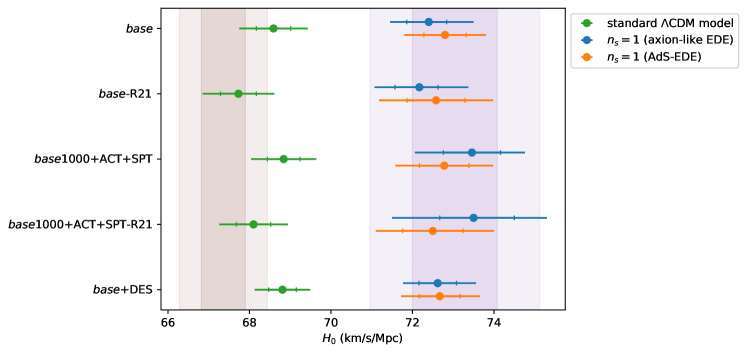
Figure 1: The posterior distribution (68% and 95% CL region shown as error bars) of $H_{0}$ for $n_{s}=1$ models under different dataset. The purple band and the brown band represent the local S$H_{0}$ES (Riess et al., 2022a) constraint (R21) and Planck 2018(Aghanim et al., 2020) constraint on $H_{0}$ (68% CL and 95% CL), respectively.

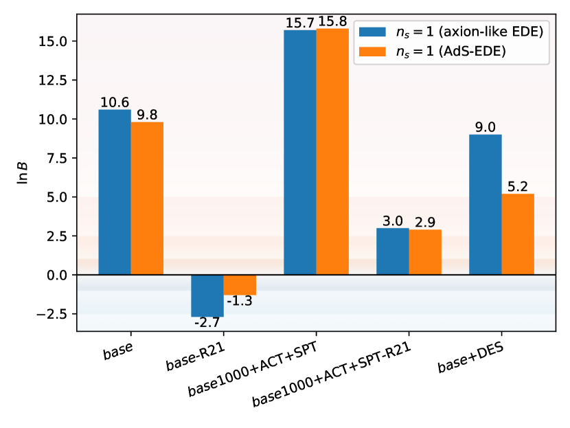
Figure 2: Bayes ratio of $n_{s}=1$ models over $\Lambda$CDM model for different datasets. Positive Bayes ratios indicate the preference for $n_{s}=1$ models. A revised version of the Jeffreys’ scale(Trotta, 2008) is also plotted as the background color.

In what follows we evaluate the Bayesian evidences for such $n_{s}=1$ models over the $\Lambda$CDM model. The widely-used Bayesian ratio is

$$B=\frac{\mathcal{Z}_{n_{s}=1\text{ (EDE)}}}{\mathcal{Z}_{\text{standard }\Lambda\text{CDM model}}}.$$ (4)

And the Bayes evidence for model $\mathcal{M}$ is

$$\mathcal{Z}_{\mathcal{M}}\equiv P(\mathbf{D}\mid\mathcal{M})=\int\mathrm{d}\Theta\mathcal{L}(\mathbf{D}\mid\Theta,\mathcal{M})\pi(\Theta\mid\mathcal{M}),$$ (5)

where $\mathcal{L}$ is the likelihood of the data $\mathbf{D}$ for model $\mathcal{M}$ and parameters $\Theta$, and $\pi$ is the prior for the model $\mathcal{M}$. However, Bayesian ratios are prior dependent. Thus we also consider another prior-independent quantity, called Suspiciousness (Lemos et al., 2020). Here, it is calculated based on the Markov chain Monte Carlo (details are presented in Appendix A) results with (Heymans et al., 2021)

$$\ln S=\left\langle\chi_{n_{s}=1\text{ (EDE)}}^{2}\right\rangle_{\mathcal{P}}/2-\left\langle\chi_{\text{standard }\Lambda\text{CDM}}^{2}\right\rangle_{\mathcal{P}}/2$$ (6)

where $\langle\,\rangle_{\mathcal{P}}$ means weighted average according to the posterior distribution. The relevant $p$-value is $p=\int_{(d_{n_{s}=1}-d_{\Lambda\text{CDM}})-2\ln S}^{\infty}\chi_{d}^{2}(x)\mathrm{d}x$, where $d=2\left(\left\langle(\ln\mathcal{L})^{2}\right\rangle_{\mathcal{P}}-\langle\ln\mathcal{L}\rangle^{2}_{\mathcal{P}}\right)$ (Handley & Lemos, 2019). As presented in Figure 1, our base dataset is Planck+BAO+SN+R21, and also they are fully compatible in $n_{s}=1$ models. The results of Bayes ratio and Suspiciousness are shown in Table 1 and Figure 2. Both indicate that $n_{s}=1$ models are favored. According to a revised version of the Jeffreys’s scale(Trotta, 2008), the evidence is very strong, $\ln{B}\simeq 10$ (note that if we exclude R21, $n_{s}=1$ models will be not favored, however, such a compare without Hubble punishment is not fair). This conclusion can also be confirmed by quite negative $\Delta\chi^{2}$, see Table 2. As a supplement, we also show the results with base1000+ACT+SPT dataset, which is the combination of base dataset with ACT DR4(Aiola et al., 2020) and SPT-3G Y1(Dutcher et al., 2021) observations, while the small scale part ($\ell>1000$) of Planck TT is cut off, as in (Hill et al., 2022; Poulin et al., 2021; La Posta et al., 2022; Smith et al., 2022b; Jiang & Piao, 2022). And it has similar conclusion.

It is well-known that weak lensing and galaxy clustering measurements for the growth of structure have $2\sim 3\sigma$ level tension with CMB, quantified as $S_{8}=\sigma_{8}(\Omega_{\text{m}}/0.3)^{0.5}$, while the injection of EDE will worsen it (Hill et al., 2020; D’Amico et al., 2021; Ivanov et al., 2020), see also(Krishnan et al., 2020; Nunes & Vagnozzi, 2021). As expected, for $n_{s}=1$ models we find $S_{8}\simeq 0.84$, see also Figure 3. However, with the base dataset+DES-Y3 (Abbott et al., 2022), we still find strong evidence ($\ln{B}>5$) for $n_{s}=1$ models. This might due to that at present DES-Y3 is not constrained well, although its uncertainty is already close to other recent observations, such as KiDS-1000 (Heymans et al., 2021).

However, we also need to note that $n_{s}$ is inversely associated with $S_{8}$ through $\Omega_{m}$, which is clearer in $\Lambda$CDM, as shown in Figure 4. Thus lower $\Omega_{m}$ can satisfy $n_{s}=1$ and a lower $S_{8}$ simultaneously, but at the cost of worse fit to BAO+SN. In fact, our $\Omega_{m}$ is shifted from $0.2995\pm 0.0054$ to $0.2911\pm 0.0039$ for $n_{s}=1$ model with axion-like EDE.

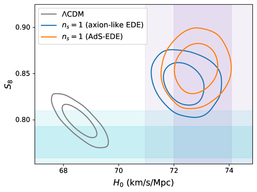
Figure 3: Posterior distribution of model parameters under the base datasets, marginalized to the $S_{8}$ - $H_{0}$ plane. The constraints on $H_{0}$ from S$H_{0}$ES (Riess et al., 2022a) (purple band) and $S_{8}$ from DES-Y3 (Abbott et al., 2022) (cyan band) are also plotted.

Table 1: Suspiciousness and relevant $p$-values of $n_{s}=1$ models over $\Lambda$CDM model for different datasets. Negative Suspiciousness indicate the preference for $n_{s}=1$ models.

Dataset	$n_{s}=1$ (axion-like EDE)		$n_{s}=1$ (AdS-EDE)
	Suspiciousness	$p$-value	Suspiciousness	$p$-value
base	$-13.5$	$2\times 10^{-7}$	$-8.5$	$2\times 10^{-5}$
base-R21	$0.0022$	$0.37$	$6.44$	$1$
$base1000$+ACT+SPT	$-17.9$	$1\times 10^{-9}$	$-13.0$	$5\times 10^{-7}$
$base1000$+ACT+SPT-R21	$-5.18$	$0.00082$	$-0.67$	$0.14$
base+DES	$-11.54$	$7\times 10^{-6}$	$-4.33$	$6\times 10^{-3}$

Table 2: $\chi^{2}_{n_{s}=1}-\chi^{2}_{\Lambda\text{CDM}}$ of the bestfit point for different $n_{s}=1$ models.

	$n_{s}=1$ (axion-like EDE)	$n_{s}=1$ (AdS-EDE)
base	$-28.4$	$-17.9$
base-R21	$-2.1$	$8.6$
$base1000$+ACT+SPT	$-37.5$	$-27.9$
$base1000$+ACT+SPT-R21	$-11.2$	$-3.1$
base+DES	$-21.2$	$-7.4$

4 Discussion and Conclusion

In conclusion, in light of recent observations, we find strong evidence for a Harrison-Zeldovich Universe. In such $n_{s}=1$ models with pre-recombination EDE, we naturally have $H_{0}\sim 73$ km/s/Mpc without well-known Hubble tension. Though DES-Y3 weakens the evidence for $n_{s}=1$ models, it is still critical to check if the joint analysis of further $S_{8}$ observations with CMB could show evidence in support of $n_{s}=1$, or one might need to rethink the physics of dark matter. It should also be noted that the high-redshift halo abundances observed by James Webb Space Telescope (JWST) appears to require a higher $n_{s}$(Klypin et al., 2021; Boylan-Kolchin, 2023) while the Lyman-alpha forest seems to prefer lower values(Iršič et al., 2017b, a; Chabanier et al., 2019; Palanque-Delabrouille et al., 2020). More studies are needed for high redshift and the tension between CMB and large-scale structure observations.

It is also significant to see, as shown in Figure 5, that $n_{s}=1$ will imprint unique signals in the CMB spectrum, especially in the small-scale part and the polarization spectrum, where the impacts of both $n_{s}=1$ and EDE are hardly balanced by the shifts of other cosmological parameters. We make a mock data forecast using CMB-S4 (Abazajian et al., 2019) . The results are shown in Table 3. The forecast with CMB-S4 indicates that if the $n_{s}=1$ model is in reality, i.e.we happened to live in such a Universe, it would be confirmed conclusively by higher-precision CMB-S4 experiment.

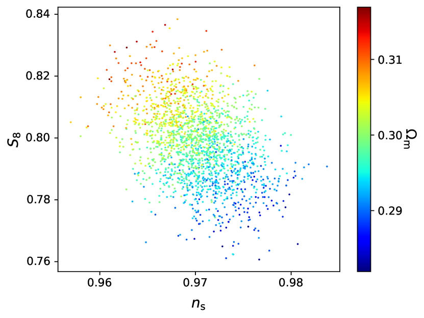
Figure 4: Posterior distribution of the $\Lambda$CDM parameters under the base dataset, marginalized to the $S_{8}$ - $n_{s}$ plane, and the relation with $\Omega_{\text{m}}$.

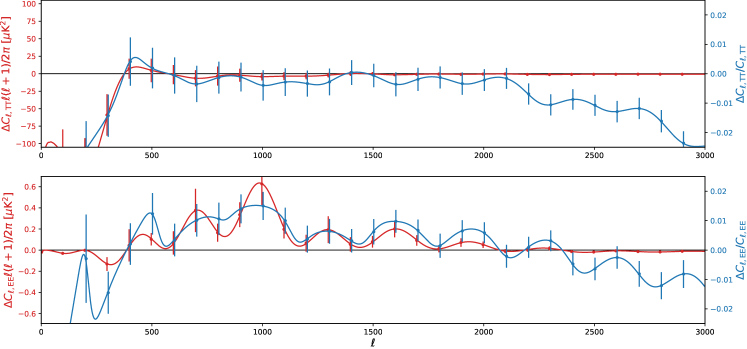
Figure 5: The residuals on the CMB power spectrum of the bestfit $\Lambda$CDM model, when fitting the mock data assuming a $n_{s}=1$ (axion-like EDE) Universe. We also plot the binned CMB-S4 forecasted error bars ($\Delta\ell=100$). The different colors represent different scaling shown in the corresponding vertical axes.

Table 3: Bayes ratios, Suspiciousness and relevant $p$-values of $n_{s}=1$ model with axion-like EDE over the $\Lambda$CDM model for the CMB-S4 mock data tests. Positive Bayes ratios and negative Suspiciousness indicate the preference for $n_{s}=1$ model.

Data	$\ln B$	Suspiciousness	$p$-value
Mock data from $\Lambda$CDM model	$-32.3$	$29.3$	$1$
Mock data from $n_{s}=1$ (axion-like EDE) model	$96.7$	$-86.2$	$1\times 10^{-39}$

Data Availability

The data underlying this article will be shared upon request to the corresponding author(s).

Appendix A Details of MCMC (Markov chain Monte Carlo) analysis

The cosmological evolution simulations and the MCMC analyses are performed using CLASS (Blas et al., 2011) and cobaya (Torrado & Lewis, 2021), respectively, and the Gelman-Rubin tests for all chains have been converged to $R-1<0.05$. The precision settings for CLASS are increased, especially for the calculation of the lensing effect since it has non-negligible effects on ground-based CMB observations, see also the appendix of (Hill et al., 2022). The injections of EDE are performed with the modified CLASS: https://github.com/PoulinV/AxiCLASS (Smith et al., 2020; Poulin et al., 2018) and https://github.com/genye00/class_multiscf. Then we use BOBYQA(Powell et al., 2009) to find the bestfit points. The prior range of parameters are summarized in Table 4 In our calculation, we fixed AdS depth to the value in (Ye & Piao, 2020). And we have confirmed that our results do not strongly depend on the choice of AdS depth.

Table 4: The prior range of parameters used in our analysis. Uniform priors are employed for all parameters.

	Parameter	Prior range
$\Lambda$CDM model parameters	$n_{s}$ (for standard $\Lambda$CDM model)	$[0.8,1.2]$
	$\log(10^{10}A_{\mathrm{s}})$	$[1.61,3.91]$
	$H_{0}$	$[20,100]$
	$\Omega_{\mathrm{b}}h^{2}$	$[0.005,0.1]$
	$\Omega_{\mathrm{c}}h^{2}$	$[0.05,0.99]$
	$\tau_{\mathrm{reio}}$	$[0.01,0.8]$
EDE parameters	$\log_{10}(z_{c})$	$[3,4]$
	$f_{\mathrm{EDE}}(z_{c})$	$[0,0.3]$
	$\Theta_{\mathrm{ini}}$ (for axion-like EDE)	$[0,3.1]$

References

- Abazajian et al. (2019) Abazajian K., et al., 2019
- Abbott et al. (2022) Abbott T. M. C., et al., 2022, Phys. Rev. D, 105, 023520
- Abdalla et al. (2022) Abdalla E., et al., 2022, JHEAp, 34, 49
- Ade et al. (2021) Ade P. A. R., et al., 2021, Phys. Rev. Lett., 127, 151301
- Aghanim et al. (2020) Aghanim N., et al., 2020, Astron. Astrophys., 641, A6
- Agrawal et al. (2019) Agrawal P., Cyr-Racine F.-Y., Pinner D., Randall L., 2019
- Aiola et al. (2020) Aiola S., et al., 2020, JCAP, 12, 047
- Akrami et al. (2020) Akrami Y., et al., 2020, Astron. Astrophys., 641, A10
- Alam et al. (2017) Alam S., et al., 2017, Mon. Not. Roy. Astron. Soc., 470, 2617
- Aylor et al. (2019) Aylor K., Joy M., Knox L., Millea M., Raghunathan S., Wu W. L. K., 2019, Astrophys. J., 874, 4
- Baxter & Sherwin (2021) Baxter E. J., Sherwin B. D., 2021, Mon. Not. Roy. Astron. Soc., 501, 1823
- Bernal et al. (2016) Bernal J. L., Verde L., Riess A. G., 2016, JCAP, 10, 019
- Beutler et al. (2011) Beutler F., et al., 2011, Mon. Not. Roy. Astron. Soc., 416, 3017
- Blas et al. (2011) Blas D., Lesgourgues J., Tram T., 2011, JCAP, 07, 034
- Boylan-Kolchin (2023) Boylan-Kolchin M., 2023, Nature Astron., 7, 731
- Chabanier et al. (2019) Chabanier S., et al., 2019, JCAP, 07, 017
- D’Amico & Kaloper (2022) D’Amico G., Kaloper N., 2022, Phys. Rev. D, 106, 103503
- D’Amico et al. (2021) D’Amico G., Senatore L., Zhang P., 2021, JCAP, 01, 006
- D’Amico et al. (2022) D’Amico G., Kaloper N., Westphal A., 2022, Phys. Rev. D, 105, 103527
- Dainotti et al. (2021) Dainotti M. G., De Simone B., Schiavone T., Montani G., Rinaldi E., Lambiase G., 2021, Astrophys. J., 912, 150
- Dainotti et al. (2022) Dainotti M. G., De Simone B., Schiavone T., Montani G., Rinaldi E., Lambiase G., Bogdan M., Ugale S., 2022, Galaxies, 10, 24
- Di Valentino et al. (2018) Di Valentino E., Melchiorri A., Fantaye Y., Heavens A., 2018, Phys. Rev. D, 98, 063508
- Di Valentino et al. (2019) Di Valentino E., Melchiorri A., Silk J., 2019, Nature Astron., 4, 196
- Di Valentino et al. (2021) Di Valentino E., et al., 2021, Class. Quant. Grav., 38, 153001
- Dutcher et al. (2021) Dutcher D., et al., 2021, Phys. Rev. D, 104, 022003
- Farren et al. (2022) Farren G. S., Philcox O. H. E., Sherwin B. D., 2022, Phys. Rev. D, 105, 063503
- Handley (2021) Handley W., 2021, Phys. Rev. D, 103, L041301
- Handley & Lemos (2019) Handley W., Lemos P., 2019, Phys. Rev. D, 100, 023512
- Harrison (1970) Harrison E. R., 1970, Phys. Rev. D, 1, 2726
- Heymans et al. (2021) Heymans C., et al., 2021, Astron. Astrophys., 646, A140
- Hill et al. (2020) Hill J. C., McDonough E., Toomey M. W., Alexander S., 2020, Phys. Rev. D, 102, 043507
- Hill et al. (2022) Hill J. C., et al., 2022, Phys. Rev. D, 105, 123536
- Iršič et al. (2017a) Iršič V., et al., 2017a, Phys. Rev. D, 96, 023522
- Iršič et al. (2017b) Iršič V., et al., 2017b, Mon. Not. Roy. Astron. Soc., 466, 4332
- Ivanov et al. (2020) Ivanov M. M., McDonough E., Hill J. C., Simonović M., Toomey M. W., Alexander S., Zaldarriaga M., 2020, Phys. Rev. D, 102, 103502
- Jiang & Piao (2021) Jiang J.-Q., Piao Y.-S., 2021, Phys. Rev. D, 104, 103524
- Jiang & Piao (2022) Jiang J.-Q., Piao Y.-S., 2022, Phys. Rev. D, 105, 103514
- Kallosh & Linde (2022) Kallosh R., Linde A., 2022, Phys. Rev. D, 106, 023522
- Karwal & Kamionkowski (2016) Karwal T., Kamionkowski M., 2016, Phys. Rev. D, 94, 103523
- Karwal et al. (2022) Karwal T., Raveri M., Jain B., Khoury J., Trodden M., 2022, Phys. Rev. D, 105, 063535
- Kelly et al. (2023) Kelly P. L., et al., 2023, Science, 380, abh1322
- Klypin et al. (2021) Klypin A., et al., 2021, Mon. Not. Roy. Astron. Soc., 504, 769
- Knox & Millea (2020) Knox L., Millea M., 2020, Phys. Rev. D, 101, 043533
- Krishnan et al. (2020) Krishnan C., Colgáin E. O., Ruchika Sen A. A., Sheikh-Jabbari M. M., Yang T., 2020, Phys. Rev. D, 102, 103525
- La Posta et al. (2022) La Posta A., Louis T., Garrido X., Hill J. C., 2022, Phys. Rev. D, 105, 083519
- Lemos et al. (2020) Lemos P., Köhlinger F., Handley W., Joachimi B., Whiteway L., Lahav O., 2020, Mon. Not. Roy. Astron. Soc., 496, 4647
- Lin et al. (2019) Lin M.-X., Benevento G., Hu W., Raveri M., 2019, Phys. Rev. D, 100, 063542
- Lin et al. (2020) Lin M.-X., Hu W., Raveri M., 2020, Phys. Rev. D, 102, 123523
- Linde (1983) Linde A. D., 1983, Phys. Lett. B, 129, 177
- Madhavacheril et al. (2023) Madhavacheril M. S., et al., 2023
- McAllister et al. (2010) McAllister L., Silverstein E., Westphal A., 2010, Phys. Rev. D, 82, 046003
- Niedermann & Sloth (2021) Niedermann F., Sloth M. S., 2021, Phys. Rev. D, 103, L041303
- Nunes & Vagnozzi (2021) Nunes R. C., Vagnozzi S., 2021, Mon. Not. Roy. Astron. Soc., 505, 5427
- Palanque-Delabrouille et al. (2020) Palanque-Delabrouille N., Yèche C., Schöneberg N., Lesgourgues J., Walther M., Chabanier S., Armengaud E., 2020, JCAP, 04, 038
- Peebles & Yu (1970) Peebles P. J. E., Yu J. T., 1970, Astrophys. J., 162, 815
- Philcox et al. (2021) Philcox O. H. E., Sherwin B. D., Farren G. S., Baxter E. J., 2021, Phys. Rev. D, 103, 023538
- Philcox et al. (2022) Philcox O. H. E., Farren G. S., Sherwin B. D., Baxter E. J., Brout D. J., 2022, Phys. Rev. D, 106, 063530
- Poulin et al. (2018) Poulin V., Smith T. L., Grin D., Karwal T., Kamionkowski M., 2018, Phys. Rev. D, 98, 083525
- Poulin et al. (2019) Poulin V., Smith T. L., Karwal T., Kamionkowski M., 2019, Phys. Rev. Lett., 122, 221301
- Poulin et al. (2021) Poulin V., Smith T. L., Bartlett A., 2021, Phys. Rev. D, 104, 123550
- Powell et al. (2009) Powell M. J., et al., 2009, Cambridge NA Report NA2009/06, University of Cambridge, Cambridge, 26
- Rashkovetskyi et al. (2021) Rashkovetskyi M., Muñoz J. B., Eisenstein D. J., Dvorkin C., 2021, Phys. Rev. D, 104, 103517
- Rezazadeh et al. (2022) Rezazadeh K., Ashoorioon A., Grin D., 2022
- Riess (2019) Riess A. G., 2019, Nature Rev. Phys., 2, 10
- Riess et al. (2022a) Riess A. G., et al., 2022a, Astrophys. J. Lett., 934, L7
- Riess et al. (2022b) Riess A. G., et al., 2022b, Astrophys. J., 938, 36
- Ross et al. (2015) Ross A. J., Samushia L., Howlett C., Percival W. J., Burden A., Manera M., 2015, Mon. Not. Roy. Astron. Soc., 449, 835
- Sakstein & Trodden (2020) Sakstein J., Trodden M., 2020, Phys. Rev. Lett., 124, 161301
- Scolnic et al. (2018) Scolnic D. M., et al., 2018, Astrophys. J., 859, 101
- Silverstein & Westphal (2008) Silverstein E., Westphal A., 2008, Phys. Rev. D, 78, 106003
- Simon et al. (2023) Simon T., Zhang P., Poulin V., Smith T. L., 2023, Phys. Rev. D, 107, 063505
- Smith et al. (2020) Smith T. L., Poulin V., Amin M. A., 2020, Phys. Rev. D, 101, 063523
- Smith et al. (2022a) Smith T. L., Poulin V., Simon T., 2022a
- Smith et al. (2022b) Smith T. L., Lucca M., Poulin V., Abellan G. F., Balkenhol L., Benabed K., Galli S., Murgia R., 2022b, Phys. Rev. D, 106, 043526
- Torrado & Lewis (2021) Torrado J., Lewis A., 2021, JCAP, 05, 057
- Trotta (2008) Trotta R., 2008, Contemp. Phys., 49, 71
- Verde et al. (2019) Verde L., Treu T., Riess A. G., 2019, Nature Astron., 3, 891
- Ye & Piao (2020) Ye G., Piao Y.-S., 2020, Phys. Rev. D, 101, 083507
- Ye et al. (2021) Ye G., Hu B., Piao Y.-S., 2021, Phys. Rev. D, 104, 063510
- Ye et al. (2022) Ye G., Jiang J.-Q., Piao Y.-S., 2022, Phys. Rev. D, 106, 103528
- Ye et al. (2023) Ye G., Zhang J., Piao Y.-S., 2023, Phys. Lett. B, 839, 137770
- Zeldovich (1972) Zeldovich Y. B., 1972, Mon. Not. Roy. Astron. Soc., 160, 1P