International Conference on Strongly Correlated Electron Systems
(SCES 2022)
Amsterdam, 24-29 July 2022 10.21468/SciPostPhysProc.?

Abstract

We consider the time-dependent thermal pure quantum state method and introduce the efficient scheme to evaluate the change in physical quantities induced by the time-dependent perturbations, which has been proposed in our previous paper [H. Taguchi et al., Phys. Rev. B 105, 125137 (2022)]. Here, we treat the Kitaev model to consider the Majorana-mediated spin transport, as an example. We demonstrate how efficient our scheme is to evaluate spin oscillations induced by the magnetic field pulse.

 

Contents

1. 1 Introduction
2. 2 Model and Method
   1. 2.1 Kitaev model with edges
   2. 2.2 Thermal Pure Quantum state method
3. 3 Results
4. 4 Conclusion

 

1 Introduction

Thermal pure quantum (TPQ) state method is one of the powerful methods to examine the thermodynamic quantities in the finite clusters [1, 2, 3] and it successfully has been applied to the quantum spin systems such as the Heisenberg models on the frustrated Kagome lattices [2, 4, 5] and the Kitaev model [6, 7, 8, 9, 10, 11, 12]. Recently, the time-dependent quantities have been examined in the framework of the TPQ method [3]. Since the TPQ state is not the eigenstate of the Hamiltonian, the expectation value, in general, depends on the time $t$ even without the time-dependent Hamiltonian, yielding to unphysical oscillations. We have proposed the scheme to reduce ill oscillations in physical quantities [13]. In this study, we briefly explain the time-dependent TPQ method and our scheme. We then demonstrate an advantage of our scheme, considering the Majorana-mediated spin transport in the Kitaev model [14, 15, 16].

This paper is organized as follows. In Sec. 2, we introduce the Kitaev model with edges and explain the TPQ method. In Sec. 3, we demonstrate the numerical results obtained by the TPQ method to clarify that our scheme has an advantage in evaluating the local physical quantities. A summary is given in the last section.

2 Model and Method

2.1 Kitaev model with edges

In the study, we consider the Kitaev model [17, 18], which is one of the quantum spin models on the honeycomb lattice and is composed of the direction dependent Ising interactions. It is known that there exists a local conserved quantity defined on each plaquette. This leads to the important feature in the Kitaev model; the quantum spin liquid state is realized, where the magnetic moments and long-range spin-spin correlations are exactly zero.

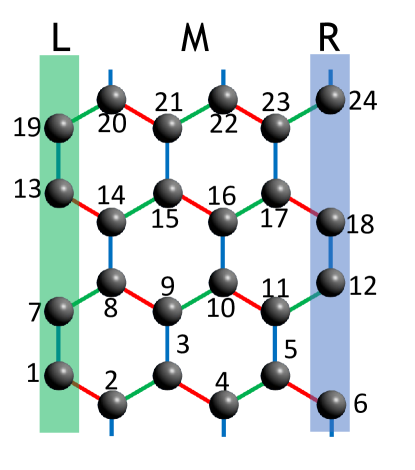
Figure 1: 24-site Kitaev cluster with armchair edges. Green, red, and blue lines indicate $x$, $y$, and $z$ bonds, respectively. The static magnetic field $h_{R}$ is applied in the right (R) region and no magnetic field is applied in the middle (M) region. A time-dependent pulsed magnetic field is introduced in the left (L) region.

Nevertheless, in the Kitaev model, the spin excitations propagate, which are mediated by the itinerant Majorana fermions [14]. This phenomenon can be observed in the Kitaev system excited by the magnetic field pulse. One of the simple setups is the system with armchair edges, as shown in Fig. 1. The system is composed of the left (L) and right (R) edge regions, and the middle (M) region, and the tiny static magnetic field is applied only to the R region. The magnetic pulsed field is introduced to the L region. The Hamiltonian is given by the static and time-dependent parts as

$$H(t) = H_{0}+H^{\prime}(t),$$ (1)

$$H_{0} = -J\sum_{\langle i,j\rangle_{x}}S_{i}^{x}S_{j}^{x}-J\sum_{\langle i,j\rangle_{y}}S_{i}^{y}S_{j}^{y}-J\sum_{\langle i,j\rangle_{z}}S_{i}^{z}S_{j}^{z}-h_{R}\sum_{i\in R}S_{i}^{z},$$ (2)

$$H^{\prime}(t) = -h_{L}(t)\sum_{i\in L}S_{i}^{z},$$ (3)

where $\langle i,j\rangle_{\mu}$ indicates the nearest-neighbor pair on the $\mu(=x,y,z)$-bonds. The $x$-, $y$-, and $z$-bonds are shown as green, red, and blue lines in Fig. 1. $S_{i}^{\mu}$ is the $\mu$ component of an $S=1/2$ spin operator at the $i$th site and $J$ is the exchange coupling between the nearest-neighbor spins. $h_{R}(=0.01J)$ represents the static magnetic field in the R region. The time-dependent magnetic field in the L region is given by the Gaussian form as

$$h_{L}(t)=\frac{A}{\sqrt{2\pi}\sigma}\exp{\left[\frac{t^{2}}{2\sigma^{2}}\right]},$$ (4)

where $A$ and $\sigma$ are strength and width of the pulse. Here, we set $\sigma=2/J$ and $A=1$. In this study, we examine the expectation value of the local quantity after the magnetic pulse is introduced in the L region.

2.2 Thermal Pure Quantum state method

Here, we explain the TPQ method to examine the expectation value of the physical quantity at finite temperatures. When $t\rightarrow-\infty$, the system is described by the static Hamiltonian $H_{0}$ and the expectation value for a certain operator $\hat{O}$ is given by the trace calculations as

$$\langle\hat{O}\rangle=\frac{1}{Z_{0}}\text{Tr}\left[\hat{O}e^{-\beta H_{0}}\right],$$ (5)

where $\beta=1/T$, $T$ is the temperature, $Z_{0}(=\text{Tr}\left[e^{-\beta H_{0}}\right])$ is the partition function. It is known that at zero temperature ($T=0$), only the ground state contributes to the expectation value. On the other hand, at finite temperatures, all eigenstates need to evaluate the expectation value, which make it hard to treat larger clusters numerically. Instead, we use the TPQ state method [1, 2]. The expectation value is represented as

$$\langle\hat{O}\rangle=\langle\Psi_{T}|\hat{O}|\Psi_{T}\rangle,$$ (6)

where $|\Psi_{T}\rangle$ is the TPQ state at the temperature $T$. In contrast to the former method, one does not have to calculate all eigenvalues and eigenstates, and thereby the TPQ state method has an advantage in treating larger systems.

We briefly describe how to construct the TPQ state. A TPQ state at $T\rightarrow\infty$ is simply given by a random vector,

$$|\Psi_{0}\rangle=\sum c_{i}|i\rangle,~{}$$ (7)

where $\{c_{i}\}$ is a set of random complex numbers satisfying $\sum_{i}|c_{i}|^{2}=1$ and $|i\rangle$ is an arbitrary Hilbert basis. By multiplying a certain TPQ state by the Hamiltonian, the TPQ states at lower temperatures are constructed. The $k$th TPQ state is represented as

$$|\Psi_{k}\rangle=\frac{(L-H_{0})|\Psi_{k-1}\rangle}{||(L-H_{0})|\Psi_{k-1}\rangle||},$$ (8)

where $L$ is a constant value, which is larger than the maximum eigenvalue of the Hamiltonian $H_{0}$. The corresponding temperature is given by

$$T_{k}=\frac{L-E_{k}}{2k},$$ (9)

where $E_{k}(=\langle\Psi_{k}|H_{0}|\Psi_{k}\rangle)$ is the internal energy. The thermodynamic quantities such as entropy and specific heat can be obtained from the internal energy and temperature. We repeat this procedure until $T_{k}=T$ and obtain the TPQ state at the temperature $T$, $|\Psi_{T}\rangle$.

The time-dependent quantities are also evaluated in the framework of the TPQ method [3]. The expectation value at time $t$ for an operator $\hat{O}$ is given as

$$\langle\hat{O}(t)\rangle = \frac{1}{Z_{0}}{\rm Tr}\left[\hat{O}(t)e^{-\beta H_{0}}\right],$$ (10)

$$= \langle\Psi_{T}|\hat{O}(t)|\Psi_{T}\rangle,$$

$$= \langle\Psi_{T}(t)|\hat{O}|\Psi_{T}(t)\rangle,$$

where $\hat{O}(t)=U^{\dagger}(t)\hat{O}U(t)$, $|\Psi_{T}(t)\rangle=U(t)|\Psi_{T}\rangle$, and $U(t)$ is the time evolution operator. Therefore, we can discuss the time-evolution of the system in terms of the time-evolution of the TPQ state. When one discusses the real-time dynamics triggered by the Hamiltonian $H^{\prime}(t)$, it is useful to examine a change in the quantities as,

$$\Delta O(t)=\langle\hat{O}(t)\rangle-\langle\hat{O}\rangle.$$ (11)

In the following, we focus on this quantity.

The TPQ method has an advantage in treating larger clusters, while we sometimes suffer from unavoidable numerical problems. When the TPQ method is applied to the finite cluster, the obtained results are sensitive to its size and/or shape. This is due to, at least, two effects. One of them is that low energy properties in the thermodynamic limit cannot be described correctly in terms of finite clusters. Therefore, the large system size dependence in the physical quantities appears at low temperatures although the TPQ method reproduces the correct results at higher temperatures. The other is the random dependence in the initial TPQ state. In general, this can be excluded, by taking a statistical average of the results for independent TPQ states. Nevertheless, we sometimes meet with difficulty in evaluating time-dependent quantities due to their large variance. This originates from the fact that each TPQ state is not an eigenstate of the Hamiltonian, leading to ill oscillations in the physical quantities with respect to time even without time-dependent perturbations, unless the quantities are conserved ones. Namely, the sample dependence is somewhat large even at high temperatures.

To avoid the latter problem, we prepare two time-dependent TPQ states from the common TPQ state as, $|\Psi_{T}(t)\rangle$ and $|\Psi_{T}^{0}(t)\rangle=U_{0}(t)|\Psi_{T}\rangle$ [13], where $U_{0}(t)$ is the time-evolution operator for the system described by $H_{0}$. Then, we calculate $\langle\langle\hat{O}(t)\rangle\rangle=\langle\Psi_{T}^{0}(t)|\hat{O}|\Psi_{T}^{0}(t)\rangle$ instead of $\langle\hat{O}\rangle$ and evaluate the change in the quantities (11), where unphysical oscillations should be canceled. This allows us to obtain $\Delta O(t)$ efficiently and to discuss correctly how the time-dependent Hamiltonian $H^{\prime}(t)$ affects the system at finite temperatures.

3 Results

We here demonstrate how efficient our scheme is to evaluate the change in the quantities at finite temperatures. To clarify this, we treat the 24-site Kitaev cluster with armchair edges (Fig. 1) and evaluate the change in the moment at the $i$th site $\Delta S_{i}^{z}(t)$ by means of the TPQ states constructed from a certain random state. The quantity is described in two distinct ways as

$$\langle S_{i}^{z}(t)\rangle-\langle S_{i}^{z}\rangle = \langle\Psi_{T}(t)|S_{i}^{z}|\Psi_{T}(t)\rangle-\langle\Psi_{T}|S_{i}^{z}|\Psi_{T}\rangle,$$ (12)

$$\langle S_{i}^{z}(t)\rangle-\langle\langle{S_{i}^{z}(t)}\rangle\rangle = \langle{\Psi_{T}(t)|S_{i}^{z}|\Psi_{T}(t)}\rangle-\langle{\Psi_{T}^{0}(t)|S_{i}^{z}|\Psi_{T}^{0}(t)}\rangle.$$ (13)

Then, we compare the results of the conventional scheme eq. (12) and our scheme eq. (13).

We calculate the change in the spin moments in the system after the magnetic pulse is introduced in the L region. In the M region, the moments are never induced due to the existence of the local conversed quantities [17]. In fact, we have confirmed the absence of the moments in the framework of the TPQ method (not shown). Now, we focus on two sites ($i=12$ and $24$) in the R region. These sites are equivalent since the Kitaev cluster treated here has a translational symmetry in the direction along the edge, as shown in Fig. 1.

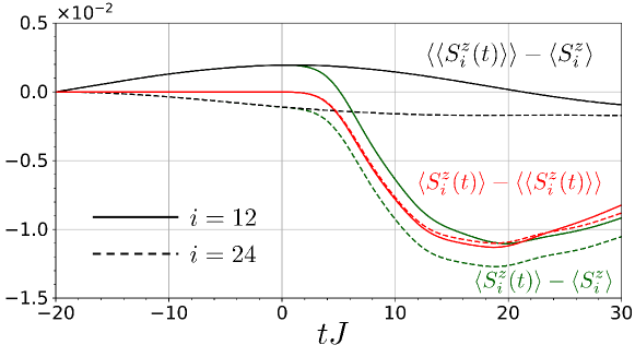
Figure 2: Green, red, and black lines indicate time-dependent quantities at $T/J=0.05$, which are calculated by the formulations eqs. (12), (13), and (14), respectively.

Figure 2 shows the change in the moment in the R region at the temperature $T/J=0.05$, which is obtained from only one TPQ state $|\Psi_{T}\rangle$. We start with the simulation from the time $t=-20/J$, where $h_{L}(t)$ is small enough. Nevertheless, we find that the changes in the spin moment described by eq. (12) are immediately induced in both sites $i=12$ and $24$ although the latter may be invisible. To understand this phenomenon, we also consider the quantity

$$\langle\langle S^{z}_{i}(t)\rangle\rangle-\langle S^{z}_{i}\rangle = \langle\Psi^{0}_{T}(t)|S_{i}^{z}|\Psi^{0}_{T}(t)\rangle-\langle\Psi_{T}|S_{i}^{z}|\Psi_{T}\rangle,$$ (14)

which is calculated in terms of the time-evolution operator $U_{0}(t)$. We find in Fig. 2 that, around $t\sim-20/J$, the quantities are the same as the results obtained from eq. (12). This means the existence of unphysical oscillations originating from the initial TPQ state. Beyond $t\sim 2/J$, we find that the difference in the results obtained from eqs. (12) and (14) becomes larger. This suggests that the physically meaningful oscillations are induced by the time-dependent perturbations (magnetic pulse introduced in the L region). In fact, by taking the statistical average in these quantities obtained from many independent TPQ states, we can confirm that the spin oscillations are correctly described by eq. (12). However, for the result obtained by one TPQ state, the induced oscillation around $t\sim 4/J$ and the initial unphysical oscillation are of the same order in this case. Therefore, the statistical average for the results obtained from a large number of TPQ states may be necessary to obtain the numerically reliable results. On the other hand, we clearly find that the formulation eq. (13) correctly describes the change in the moment; no oscillation behavior appears before the Gaussian pulse is introduced in the L region, and the quantities for both sites are almost the same, which is consistent with the symmetry argument in the system. It is naively expected that the accurate results should be obtained by the statistical average for a smaller number of samples. Therefore, we can say that our scheme (13) has an advantage in evaluating the local physical quantities.

4 Conclusion

We have treated the Kitaev model with edges to examine the time-evolution of the spin moments by means of the time-dependent thermal pure quantum state method. We have explained the detail of our scheme proposed in our previous paper, where two kinds of the time-evolution operators are applied to the common TPQ state. Then, we have demonstrated that ill oscillations in the physical quantities, which originate from the fact that each TPQ state is not an eigenstate and causes a problem in the conventional time-evolution scheme, are suppressed. We have evaluated the change in the moment at each site in the Kitaev model.

References

- [1] S. Sugiura and A. Shimizu, Thermal pure quantum states at finite temperature, Phys. Rev. Lett. 108, 240401 (2012), 10.1103/PhysRevLett.108.240401.
- [2] S. Sugiura and A. Shimizu, Canonical thermal pure quantum state, Phys. Rev. Lett. 111, 010401 (2013), 10.1103/PhysRevLett.111.010401.
- [3] H. Endo, C. Hotta and A. Shimizu, From linear to nonlinear responses of thermal pure quantum states, Phys. Rev. Lett. 121, 220601 (2018), 10.1103/PhysRevLett.121.220601.
- [4] K. Morita and T. Tohyama, Finite-temperature properties of the kitaev-heisenberg models on kagome and triangular lattices studied by improved finite-temperature lanczos methods, Phys. Rev. Research 2, 013205 (2020), 10.1103/PhysRevResearch.2.013205.
- [5] T. Misawa, Y. Motoyama and Y. Yamaji, Asymmetric melting of a one-third plateau in kagome quantum antiferromagnets, Phys. Rev. B 102, 094419 (2020), 10.1103/PhysRevB.102.094419.
- [6] Y. Yamaji, T. Suzuki, T. Yamada, S.-i. Suga, N. Kawashima and M. Imada, Clues and criteria for designing a kitaev spin liquid revealed by thermal and spin excitations of the honeycomb iridate , Phys. Rev. B 93, 174425 (2016), 10.1103/PhysRevB.93.174425.
- [7] H. Tomishige, J. Nasu and A. Koga, Interlayer coupling effect on a bilayer kitaev model, Phys. Rev. B 97, 094403 (2018), 10.1103/PhysRevB.97.094403.
- [8] A. Koga, S. Nakauchi and J. Nasu, Role of spin-orbit coupling in the kugel-khomskii model on the honeycomb lattice, Phys. Rev. B 97, 094427 (2018), 10.1103/PhysRevB.97.094427.
- [9] A. Koga, H. Tomishige and J. Nasu, Ground-state and thermodynamic properties of an s = 1 kitaev model, J. Phys. Soc. Jpn. 87(6), 063703 (2018), 10.7566/JPSJ.87.063703.
- [10] J. Oitmaa, A. Koga and R. R. P. Singh, Incipient and well-developed entropy plateaus in spin- kitaev models, Phys. Rev. B 98, 214404 (2018), 10.1103/PhysRevB.98.214404.
- [11] T. Suzuki and Y. Yamaji, Temperature dependence of heat capacity in the kitaev-heisenberg model on a honeycomb lattice, J. Phys. Soc. Jpn. 88(11), 115001 (2019), 10.7566/JPSJ.88.115001.
- [12] A. Koga and J. Nasu, Residual entropy and spin fractionalizations in the mixed-spin kitaev model, Phys. Rev. B 100, 100404(R) (2019), 10.1103/PhysRevB.100.100404.
- [13] H. Taguchi, Y. Murakami and A. Koga, Thermally enhanced majorana-mediated spin transport in the kitaev model, Phys. Rev. B 105, 125137 (2022), 10.1103/PhysRevB.105.125137.
- [14] T. Minakawa, Y. Murakami, A. Koga and J. Nasu, Majorana-mediated spin transport in kitaev quantum spin liquids, Phys. Rev. Lett. 125, 047204 (2020), 10.1103/PhysRevLett.125.047204.
- [15] A. Koga, T. Minakawa, Y. Murakami and J. Nasu, Spin transport in the quantum spin liquid state in the s = 1 kitaev model: Role of the fractionalized quasiparticles, J. Phys. Soc. Jpn 89(3), 033701 (2020), 10.7566/JPSJ.89.033701.
- [16] H. Taguchi, Y. Murakami, A. Koga and J. Nasu, Role of majorana fermions in spin transport of anisotropic kitaev model, Phys. Rev. B 104, 125139 (2021), 10.1103/PhysRevB.104.125139.
- [17] A. Kitaev, Anyons in an exactly solved model and beyond, Ann. Phys. 321(1), 2 (2006), https://doi.org/10.1016/j.aop.2005.10.005.
- [18] Y. Motome and J. Nasu, Hunting majorana fermions in kitaev magnets, J. Phys. Soc. Jpn 89(1), 012002 (2020), 10.7566/JPSJ.89.012002.