Outlier-Insensitive Kalman Filtering using NUV Priors

Abstract

The kf (kf) is a widely-used algorithm for tracking the latent state of a dynamical system from noisy observations. For systems that are well-described by lg ss models, the kf minimizes the mse (mse). However, in practice, observations are corrupted by outliers, severely impairing the kf’s performance. In this work, an outlier-insensitive kf is proposed, where robustness is achieved by modeling each potential outlier as a nuv (nuv). The nuv variances are estimated online, using both em (em) and am (am). The former was previously proposed for the task of smoothing with outliers and was adapted here to filtering, while both em and am obtained the same performance and outperformed the other algorithms, the AM approach is less complex and thus requires $40\%$ less runtime. Our empirical study demonstrates that the mse of our proposed outlier-insensitive kf outperforms previously proposed algorithms, and that for data clean of outliers, it reverts to the classic kf, i.e., mse optimality is preserved.

Index Terms—  kf, outliers, am

1 Introduction

Se of dynamical systems from noisy observations plays a key role in various scientific and technological fields such as radar target tracking, complex image processing, navigation, and positioning [1]. The celebrated kf [2] is an efficient recursive state estimation algorithm that is mse optimal for dynamical systems obeying a lg ss (ss) model. However, the quadratic form of its objective, i.e., mse, makes it sensitive to deviations from nominal noise. Thus, the kf is severely impaired when outliers are present in the measurements [3, 4]. As sensory data is often populated with outliers, robustness to outliers is essential [5, 6, 7]. A common approach for dealing with outliers is to detect and then disregard influential observations. Such detection can be achieved using appropriate statistical diagnostics [8] on the posterior distribution, e.g., $Z\textrm{-test}$ [9] and $\chi^{2}\textrm{-test}$ [10, 11]. The main drawbacks of these approaches are that they need to be carefully tuned for a required false alarm, and that potentially useful outlier information is not accounted for in the estimation process. Alternatively, one can limit the effect of outliers by reweighting the covariance of the observation noise at each data sample when estimating the current state [5, 6]. These techniques require careful tuning of multiple hyperparameters to operate reliably as well. A different approach formulates the kf as a linear regression problem, detecting outliers via a sparsifying $\ell_{1}$-penalty [4, 12], tackled via optimization techniques, which may be computationally complex.

In this work, a new approach for oikf (oikf) is proposed that leverages ideas from sparse Bayesian learning [13]. Here, each potential outlier is modeled as a nuv [14, 15, 7], i.e., an additive component on top of the observation noise. nuv incorporation effectively yields a modified overall sparsity-aware objective [14], which is shown to yield a robust outlier detection statistical test with a relatively low false alarm. When an outlier is reliably detected, we incorporate its variance into the overall covariance matrix of the observation noise, thereby balancing its contribution to the information fusion (i.e., update) step in the kf, and the outlier information is used in the se process.

To estimate the nuv online, we first adapt the em algorithm [16, 17, 18], which was previously proposed for offline smoothing [7], to the online filtering task. em is based on computing second-order moments, i.e., the full state observation posterior covariance. We then present an implementation, which has not been considered to date, using a simpler am algorithm [19, 20, 21]. Unlike em, am uses only first-order moments as an empirical surrogate for outlier detection, without sacrificing performance and with improved robustness. We evaluate the oikf for tracking based on the wna (wna) motion model with outliers [22]. We empirically demonstrate the superiority of our proposed algorithm compared to previous robust variants of the kf, achieving improved performances with low complexity operations.

The rest of this paper is organized as follows: Section 2 formulates the system and the kf with outliers. Section 3 presents the oikf with its estimation for the outlier’s variance, and Section 4 empirically evaluates our methods.

2 System Model and the Kalman Filter

ss models in dt are a common characterization of dynamical systems [22]. Such representations capture the relationship between an unknown latent state vector $\mathbf{x}_{t}$ and an observed vector $\mathbf{y}_{t}$, where $t\in\mathbb{Z}$ is the time index. Here, a Gaussian and continuous ss model is considered, namely

$$\mathbf{x}_{t} =\mathbf{F}\cdot{\mathbf{x}_{t-1}}+\mathbf{e}_{t},\quad\,\,\,\,\,\,\mathbf{e}_{t}\sim\mathcal{N}\left(\mathbf{0},\mathbf{Q}\right),\quad\mathbf{x}_{t}\in\mathbb{R}^{m}$$ (1a)

$$\mathbf{y}_{t} =\mathbf{H}\cdot\mathbf{x}_{t}+\mathbf{z}_{t}+\mathbf{u}_{t},\,\,\,\,\mathbf{z}_{t}\sim\mathcal{N}\left(\mathbf{0},\mathbf{R}\right),\quad\mathbf{y}_{t}\in\mathbb{R}^{n}.$$ (1b)

In (1a), the state evolves by an evolution matrix $\mathbf{F}$ and by awgn (awgn) $\mathbf{e}_{t}$ with covariance matrix $\mathbf{Q}$. In (1b), the state observations are generated by the linear mapping $\mathbf{H}$ corrupted by an awgn $\mathbf{z}_{t}$ with a diagonal covariance matrix $\mathbf{R}=\textrm{diag}\left(\mathbf{r}^{2}\right)$, and by additive outlier impulsive noise $\mathbf{u}_{t}$ with an unknown distribution. The kf is an efficient online recursive filter that estimates the state $\mathbf{x}_{t}$ from the observations $\{\mathbf{y}_{\tau}\}_{\tau\leq t}$. It is mse optimal for the ss model (1) without the outliers $\mathbf{u}_{t}$. It can be conceptualized as a two-step procedure in each time step $t$, predict and update, in which the joint probability distribution over the variables is computed, using the first- and second-order moments of the Gaussian distribution. In the predict step, the prior distribution is computed, namely

$$\hat{\mathbf{x}}_{t\left|t-1\right.} =\mathbf{F}\cdot{\hat{\mathbf{x}}_{t-1}},\hskip 12.80365pt\bm{\Sigma}_{t\left|t-1\right.}\!=\!\mathbf{F}\cdot\bm{\Sigma}_{t-1}\cdot\mathbf{F}^{\top}\!+\!\mathbf{Q},$$ (2a)

$$\hat{\mathbf{y}}_{t\left|t-1\right.} =\mathbf{H}\cdot{\hat{\mathbf{x}}_{t\left|t-1\right.}},\hskip 5.69046pt\mathbf{S}_{t\left|t-1\right.}\!=\!\mathbf{H}\cdot\bm{\Sigma}_{t\left|t-1\right.}\cdot\mathbf{H}^{\top}\!+\!\mathbf{R}.$$ (2b)

In the update step the posterior distribution is computed by fusing the new observation $\mathbf{y}_{t}$ with the previously predicted prior $\hat{\mathbf{x}}_{t\left|t-1\right.}$, where the kg (kg) matrix $\mathbfcal{K}_{t}$ is used to balance the contributions of both parts, namely

$$\hat{\mathbf{x}}_{t}=\hat{\mathbf{x}}_{t\left|t-1\right.}+\mathbfcal{K}_{t}\cdot\Delta\mathbf{y}_{t},\quad{\bm{\Sigma}}_{t}\!=\!{\bm{\Sigma}}_{t\left|t-1\right.}\!-\!\mathbfcal{K}_{t}\cdot{\mathbf{S}}_{t\left|t-1\right.}\cdot\mathbfcal{K}^{\top}_{t},$$ (3)

$$\mathbfcal{K}_{t}={\bm{\Sigma}}_{t\left|t-1\right.}\cdot{\mathbf{H}^{\top}}\cdot{\mathbf{S}}^{-1}_{t\left|t-1\right.},\quad\Delta\mathbf{y}_{t}=\mathbf{y}_{t}-\hat{\mathbf{y}}_{t\left|t-1\right.}.$$ (4)

3 OUTLIER-INSENSITIVE KALMAN filtering

Next we propose our outlier-robust online filter. In Subsection 3.1 we present the nuv modeling. Then we present the oikf algorithm in Subsection 3.2, after which we derive two considered methods for nuv estimation based on em (Subsection 3.3) and am (Subsection 3.4).

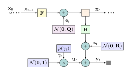
Fig. 1: Factor graph of the system model at time step $t$

3.1 NUV Modeling

Given an observation sample $\mathbf{y}_{t}$ (1b), we define $\mathbf{v}_{t}$ to be the error vector as the sum of two independent sources: the observation noise $\mathbf{z}_{t}$ and the outlier-causing impulsive noise $\mathbf{u}_{t}$, modeled as nuv with unknown variance vector ${\boldsymbol{\gamma}}^{2}_{t}$. Thus, the covariance of $\mathbf{v}_{t}$, $\mathbf{\Gamma}_{t}$, is diagonal and comprises the sum of variances of the two noise sources, namely

$$\mathbf{v}_{t} \triangleq\mathbf{y}_{t}-\mathbf{H}\cdot\mathbf{x}_{t}=\mathbf{z}_{t}+\mathbf{u}_{t},\quad\mathbf{u}_{t}\sim\mathcal{N}\left(\mathbf{0},{\boldsymbol{\gamma}}^{2}_{t}\right),$$ (5a)

$$\mathbf{v}_{t} \sim\mathcal{N}\left(\mathbf{0},\mathbf{\Gamma}_{t}\right),\quad\mathbf{\Gamma}_{t}=\textrm{diag}\left({\bm{\nu}}^{2}_{t}\right),\quad{\bm{\nu}}^{2}_{t}\triangleq\mathbf{r}^{2}+{\boldsymbol{\gamma}}^{2}_{t}.$$ (5b)

The motivation for utilizing the nuv framework stems from its ability to systematically incorporate interference of a bursty nature [14, 15], and is thus useful for handling outliers with sparse ls (quadratic) models [7]. The incorporation of the nuv representation to the overall ss model (1), is illustrated as a factor graph [23] in Figure 1.

3.2 OIKF Algorithm

The proposed oikf uses map (map) estimation to instantaneously estimate the unknown variance ${\boldsymbol{\gamma}}^{2}_{t}$. By either applying em or am in each time step $t$, we obtain an estimate for the variance. In the em version, the second-order moment $\mathbf{\nu}_{t}$ (5b) is directly estimated, while in am version it is obtained from estimating $\mathbf{v}_{t}$ (5a), i.e., from the first-order moment. The oikf thus uses

$${\hat{\boldsymbol{\gamma}}}^{2}_{t}=\max\left\{\bm{\nu}_{t}^{2}-\mathbf{r}^{2},0\right\},\hskip 4.97931pt\bm{\nu}_{t}^{2}=\left\{\textrm{EM}:\hat{\bm{\nu}}_{t}^{2},\textrm{AM}:\mathbf{\hat{v}}^{2}_{t}\right\}.$$ (6)

A key property of the map estimator (6) is that it tends to be sparse [14], thus providing a robust statistical test to detect the presence of outliers. Due to the sparsity property, in most of the time steps, outliers are not detected, and filtering coincides with the standard kf, thus preserving its optimality for data without outliers. When outlier is detected, namely, when $\hat{\boldsymbol{\gamma}}^{2}_{t}\neq\mathbf{0}$, its contribution to the update step is balanced via its estimated variance; it is integrated into the overall error covariance $\mathbf{\Gamma}_{t}$, which in turn becomes the observation noise and therefore affects the kg in the update equation.

The above procedure is repeated iteratively, and the pseudo-code for the proposed oikf is summarized in Algorithm 1. It can be done for fixed $N$ iterations, or until convergence. In [7], $\hat{\boldsymbol{\gamma}}^{2}_{t}$ was initialized to $\mathbf{0}$. Here, empirical experience suggests to initialize it to the value of the prior moments. While retaining performance, it converges faster.

Algorithm 1 oikf at time instance $t$

Number of iterations $N$

Predict: Estimate a priori for $\mathbf{\hat{x}}_{t\left|t-1\right.}^{i=0},\mathbf{\bm{\Sigma}}_{t\left|t-1\right.}^{i=0}$ via (2a)

for $i=0,...,N-1$ do

    AM: Compute $\mathbf{\hat{v}}_{t}^{i}=\mathbf{y}_{t}-\mathbf{H}\cdot\mathbf{\hat{x}}_{t}^{i}$

             Estimate $\left(\hat{\boldsymbol{\gamma}}^{i}_{t}\right)^{2}$ via (15)

    EM: Estimate $\left(\hat{\boldsymbol{\gamma}}^{i}_{t}\right)^{2}$ via (10) with the $2$nd-order

              moment ${\hat{\mathbf{X}}_{t}^{i}}$ as in (8)

    Compute $\mathbf{\Gamma}_{t}^{i}=\textnormal{diag}\left(\mathbf{r}^{2}+\left(\hat{\boldsymbol{\gamma}}^{i}_{t}\right)^{2}\right)$

    Compute $\mathbf{\hat{y}}_{t\left|t-1\right.}^{i},\mathbf{S}_{t\left|t-1\right.}^{i}$ via  (2b) with $\mathbf{R}=\mathbf{\Gamma}_{t}^{i}$.

    Update: Estimate a posteriori for $\mathbf{\hat{x}}_{t}^{i},\bm{\Sigma}_{t}^{i}$ via (3)

end for

3.3 Expectation Maximization

For an observation sample $\mathbf{y}_{t}$, the map estimate for $\hat{\boldsymbol{\gamma}}^{2}_{t}$ is

$${\hat{\boldsymbol{\gamma}}_{t}^{2}}\left(\mathbf{y}_{t}\right)={\arg}\max_{\boldsymbol{\gamma}^{2}_{t}}p\left(\mathbf{y}_{t}\left|\boldsymbol{\gamma}^{2}_{t}\right.\right)\cdot p\left(\boldsymbol{\gamma}^{2}_{t}\right).$$ (7)

To compute the map estimate using EM, we assume a plain nuv, i.e., a uniform prior $p\left(\boldsymbol{\gamma}^{2}_{t}\right)\propto 1$ [14]. We can now evaluate the standard em by alternating between the E-step, i.e., the conditional expectation, and the M-step, i.e., maximizing this expression with respect to $\boldsymbol{\gamma}^{2}_{t}$. Here, the expectation step corresponds to the kf, from which we get first- and second-order posterior moments, namely

$$\hat{\mathbf{x}}_{t}^{i},\qquad{\hat{\mathbf{X}}_{t}^{i}}\triangleq\bm{\Sigma}^{i}_{t}+\hat{\mathbf{x}}_{t}^{i}\cdot{\hat{\mathbf{x}}^{i}_{t}}^{\top}.\vspace{-0.9mm}$$ (8)

The maximization step corresponds to recovering the covariance  (5b) using the following estimate [7, 18]:

$${\mathbf{\hat{\Gamma}}_{t}^{i}}=\mathbf{y}_{t}\cdot\mathbf{y}^{\top}_{t}-\mathbf{H}\cdot\hat{\mathbf{x}}_{t}^{i}\cdot{\mathbf{y}^{\top}_{t}}-{\mathbf{y}}_{t}\cdot{{\mathbf{\hat{x}}^{i}_{t}}}^{\top}\cdot\mathbf{H}^{\top}-\mathbf{H}\cdot{\hat{\mathbf{X}}_{t}^{i}}\cdot\mathbf{H}^{\top}.$$ (9)

We exploit the fact that $\mathbf{{\Gamma}}_{t}$ in (5b) is diagonal, to estimate the variance $\left(\mathrm{\hat{\nu}}^{i}_{t,k}\right)^{2}$ for each dimension $k\in\{1,\dots,n\}$ in a scalar manner. Since ${\gamma}_{t,k}^{2}$ is non-negative, we get the following expression for its estimate:

$$\left({\hat{\gamma}}^{i}_{t,k}\right)^{2}=\max\left\{\left({\hat{\nu}}^{i}_{t,k}\right)^{2}-\mathrm{r}_{k}^{2},0\right\}.$$ (10)

This demonstrates the sparsifying property of the nuv modeling, maybe more specifically the map estimate for $\mathrm{u}_{t,k}$ from $\hat{\gamma}^{2}_{t,k}$ [14] is

$$\hat{\mathrm{u}}_{t,k} =\mathrm{v}_{t,k}\cdot\frac{\hat{\gamma}^{2}_{t,k}}{\hat{\gamma}^{2}_{t,k}+{\mathrm{r}^{2}_{k}}}=\max\left\{\mathrm{v}_{t,k}\cdot\frac{\hat{\nu}^{2}_{t,k}-{\mathrm{r}^{2}_{k}}}{\hat{\nu}^{2}_{t,k}},0\right\}.$$ (11)

Namely, $\hat{\gamma}^{2}_{t,k}$ leads to $\hat{\mathrm{u}}_{t,k}=0$. When the outlier is identified as zero, oikf coincides with the kf.

3.4 Alternating Maximization

We next describe an iterative am method to compute the joint map estimate based on the nuv representation [15]

$$[\hat{\mathbf{v}}_{t},\hat{\mathrm{\boldsymbol{\gamma}}}^{2}_{t}](\mathbf{y}_{t})\!=\!\underset{{\mathbf{v}_{t},\boldsymbol{\gamma}^{2}_{t}}}{\arg\max}\,p\left({\mathbf{y}_{t}\left|\mathbf{v}_{t}\right.}\right)\cdot p\big{(}\mathbf{v}_{t}\big{|}{\boldsymbol{\gamma}^{2}_{t}}\big{)}\cdot p\left(\boldsymbol{\gamma}^{2}_{t}\right).$$ (12)

am iterates between a maximization step over the error state ${\mathbf{v}}_{t}$ with fixed variance ${\boldsymbol{\gamma}^{2}_{t}}$:

$$\hat{\mathbf{v}}_{t}\!=\!\underset{{\mathbf{v}_{t}}}{\arg\max}\,p\left({\mathbf{y}_{t}\left|\mathbf{v}_{t}\right.}\right)\cdot p\left(\mathbf{v}_{t}\left|\boldsymbol{\gamma}\right.^{2}_{t}\right)\cdot p\left(\boldsymbol{\gamma}^{2}_{t}\right),$$ (13)

and a maximization step over the unknown variance ${\boldsymbol{\gamma}^{2}_{t}}$ based on $\mathbf{v}_{t}$, i.e., finding

$$\hat{\boldsymbol{\gamma}}^{2}_{t}=\underset{{\boldsymbol{\gamma}^{2}_{t}}\geq 0}{\arg\max}\,p\left(\mathbf{v}_{t}\left|\boldsymbol{\gamma}\right.^{2}_{t}\right)\cdot p\left(\boldsymbol{\gamma}^{2}_{t}\right).\vspace{-3mm}$$ (14)

Similarly to our derivation of em in Subsection 3.3, we assume a uniform prior on ${\boldsymbol{\gamma}}_{t}^{2}$. However, while em utilizes estimates of both the first- and second-order moments of the states, namely, $\hat{\mathbf{x}}_{t}^{i}$ and ${\hat{\mathbf{X}}_{t}^{i}}$ (8), am uses only $\hat{\mathbf{x}}_{t}^{i}$.

For convenience, we formulate the second step in a scalar manner, which extends to multivariate observations by assuming that the observation noise $\mathbf{z}_{t}$ and the outlier $\mathbf{u}_{t}$ in each dimension are independent. In particular, by replacing $\mathbf{v}_{t}$ in (14) with its instantaneous estimate $\mathbf{\hat{v}}_{t}^{i}=\mathbf{y}_{t}-\mathbf{H}\cdot\mathbf{\hat{x}}_{t}^{i}$ computed from the kf, we obtain the following update rule for the $k$th entry of the unknown variance

$$\left({\hat{\gamma}}^{i}_{t,k}\right)^{2}\!=\!\max\left\{{({\mathrm{\hat{v}}^{i}_{t,k}})^{2}\!-\!{\mathrm{r}^{2}_{k}},0}\right\}.$$ (15)

We obtain an analytic expression of $\hat{\gamma}^{2}_{t,k}$ for the update step, which is parameter-free. Furthermore, combining am with the nuv-prior results in an equivalent cost function $\mathcal{L}\left(\mathbf{v}_{t}\right)\triangleq-\log\,p\left(\mathbf{v}_{t}\right)$ that is non-convex [15]. This is equivalent loss function useful for sparse ls models, e.g., kf with outliers [15], and $\hat{\boldsymbol{\gamma}}_{k}^{2}$ is likely to be sparse, following the same arguments as in Subsection 3.3.

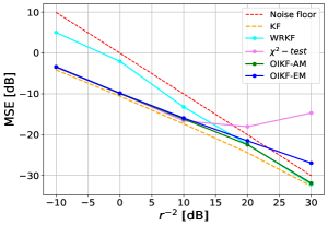
(a) Noisy data clean of outliers

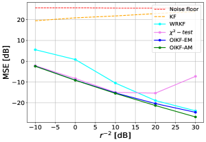
(b) Noisy data with outliers

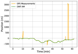
(c) Vehicle estimated trajectory

Fig. 2: Sub-Fig. 2(a) and 2(b) present the obtained MSE for different algorithms and Sub-Fig. 2(c) presents the measured vehicle position obtained from the noisy GPS readings (orange line), and the trajectory estimated by our oikf-am (green dashed line).

3.5 Discussion

The proposed oikf is designed to track in the presence of outliers by iteratively refining its update step with map estimation of the outlier variance. Both em and am algorithms can be used to tackle this map estimation, which arises from the nuv modelling. The main difference between the algorithms is that em uses the second-order moment of the state vector, while am uses the first-order moment only, hence it does not require the posterior covariance matrix $\bm{\Sigma}_{t}$ in each iteration. Consequently, am avoids possibly unnecessary heuristics in the model noise, making it more robust compared to em, as empirically demonstrated in Section 4. The fact that am does not explicitly rely on the second-order moments is expected to facilitate its augmentation with trainable data-driven variants of the Kalman filter, e.g., [24, 25, 26]. Such a fusion of oikf with data-aided computations, which we intend to explore in future work, bears the potential of facilitating robust filtering in partially known ss models.

oikf provides a degree of freedom in choosing the prior of $\boldsymbol{\gamma}_{k}^{2}$. We chose it to be uniform, which is parameter free, and can be shown to effectively modify the overall loss function to account for sparse outliers [15]. Alternative settings of this prior would result in different effective loss functions such as the convex Huber cost function [27, 15]. We leave the investigation of oikf with different priors to future work.

4 Empirical Evaluation

To evaluate the proposed oikf-am and oikf-em, we tested these algorithms on a standard localization task. We compare our proposed algorithms performance in terms of position error to the following alternative algorithms: $1)$ the standard kf; $2)$ the well-known $\chi^{2}\textrm{-test}$ [10] (with a $95\%$ confidence level); $3)$ the weighted covariance methods, i.e., the WRKF from [5]; and $4)$ the ORKF from [6]. We evaluate these algorithms in two settings: A synthetic dataset generated from a known SS model, and real-world dynamics data based on the Michigan NCLT dataset [28]. In both cases, the state vector is given by $\mathbf{x}=\left(\mathrm{p,v}\right)^{\top}$, where $\mathrm{p}$ and $\mathrm{v}$ are the position and velocity, respectively.

For the synthetic data we define the dynamic wna model [22], defined by a linear ss model. The system is fully observable, thus the observation matrix is the identity matrix $\mathbf{H}=\mathbf{I}_{n}$ and the observation noise covariance matrix is defined as $\mathbf{R}=\mathrm{r}^{2}\cdot\mathbf{I}_{n}$. The state-evolution noise variance $\textnormal{q}^{2}$ is set to a constant value of $-10\left[\textrm{dB}\right]$. Uncertainty in the dynamics and measurements is accounted for by Gaussian i.i.d input, state, and measurements noise, whereas the outliers are modeled with intensity sampled from a Rayleigh distribution $\mathcal{RAY}\left(\beta\right)$ with scale parameter $\beta=30$. The outliers’ time steps are drawn from a Bernoulli distribution, namely $\mathcal{B}\left(p\right)$, where ${p}$ is set to 0.2. For the real-world data we use the NCLT dataset from session with date 2013-04-05, which contains noisy GPS (GPS) readings and the corresponding ground truth location of a moving Segway robot. For the filter process, we define the dynamic wna model[22]. The only observable output is the GPS position, thus the observation matrix is $\mathbf{H}=\left(\begin{matrix}1&0\end{matrix}\right)$ and the observation noise covariance matrix is $\mathbf{R}={\mathrm{r}^{2}}$.

The results reported in Fig. 2(a) examine the performance for synthetic data clean of outliers. In this case, it is shown that the oikf-am achieves the optimal minimal mse bound, as most $\hat{\gamma}^{2}_{t}$ values are estimated to be zero, which means the model turns back to be the kf. When the synthetic data is populated with outliers, the oikf-am has the best performance in terms of mse compared to other algorithms for different values of observation noise variance $\mathrm{r}^{2}$, as presented in Fig  2(b). More specifically, it coincides with the oikf-em, and even outperforms it for low observation noise, without using a second-order moment as in em.

We proceed to the NCLT data set and demonstrate the tracking of a single trajectory in Fig. 2(c). We observe in Fig. 2(c) the robustness of oikf-am in estimating the position from real-world data while reliably smoothing the outliers. Table 1 presents the obtained position rmse (rmse) and mse for each of the algorithms when the observation noise variance is set to $\mathrm{r}^{2}=3^{2}$, which is a GPS ”textbook” error, while $\mathrm{r}^{2}$ is selected for each algorithm separately by grid search to yield the lowest mse. For both scenarios $\mathrm{q}^{2}$ was optimized by grid search. We can see in Table 1 that our proposed oikf-em and oikf-am produce the lowest estimation errors for both settings, when the latter coincides with the oikf-em, even without using the second-order moment. Furthermore, the OIKF-AM exhibits the shortest runtime in the domain of algorithms for outlier detection and weighting (except the $\chi^{2}\textrm{-test}$ that only detects and then rejects the outliers). For instance, in comparison to our other suggested method the oikf-em, the oikf-am showcases an almost $40\%$ reduced runtime compared to it.

Table 1: Position error for different values of $\mathrm{r}^{2}$

	${\mathrm{r}^{2}=3^{2}}$		optimal ${\mathrm{r}^{2}}$		Runtime
	rmse[m]	mse$\left[\textrm{dB}\right]$	rmse[m]	mse$\left[\textrm{dB}\right]$	[ms]
Noisy GPS	349.31	50.86	349.31	50.86	-
kf	94.35	39.49	92.28	39.3	0.05
ORKF	75.79	37.59	27.74	28.86	2.83
$\chi^{2}\textrm{-test}$	45.3	33.12	14	22.92	0.06
oikf-am	10.87	20.72	10.38	20.33	0.28
oikf-em	10.73	20.61	10.35	20.29	0.44

5 Conclusions

In this work we derived a novel approach for outlier insensitive Kalman-filtering oikf. Based on sparse Bayesian learning concepts, we modeled outliers as NUV with am or em approaches, resulting in a sparse outlier detection. Both algorithms are parameter-free and amount essentially to a short iterative process during the update step of the kf. The presented empirical evaluations demonstrate that oikf-am and oikf-em present better performance compared to the other algorithms in terms of mse and rmse, highlighting the robustness and accuracy of oikf for systems that rely on high-quality sensory data.

References

- [1] J. Durbin and S. J. Koopman, Time series analysis by state space methods. Oxford University Press, 2012.
- [2] R. E. Kalman, “A new approach to linear filtering and prediction problems,” Journal of Basic Engineering, vol. 82, no. 1, 1960.
- [3] A. Aravkin, J. V. Burke, L. Ljung, A. Lozano, and G. Pillonetto, “Generalized Kalman smoothing: Modeling and algorithms,” Automatica, vol. 86, 2017.
- [4] S. Farahmand, G. B. Giannakis, and D. Angelosante, “Doubly robust smoothing of dynamical processes via outlier sparsity constraints,” IEEE Trans. Signal Process., vol. 59, no. 10, 2011.
- [5] J. A. Ting, E. Theodorou, and S. Schaal, “A Kalman filter for robust outlier detection,” IEEE IROS, 2007.
- [6] G. Agamennoni, J. I. Nieto, and E. M. Nebot, “An outlier-robust Kalman filter,” IEEE ICRA, 2011.
- [7] F. Wadehn, L. Bruderer, J. Dauwels, V. Sahdeva, H. Yu, and H. A. Loeliger, “Outlier-insensitive Kalman smoothing and marginal message passing,” 24th EUSIPCO, Aug 2016.
- [8] R. M. Gray, An introduction to statistical signal processing. Cambridge University Press, 2004.
- [9] P. J. Rousseeuw and M. Hubert, “Robust statistics for outlier detection,” Wiley Interdisciplinary Reviews: Data Mining and Knowledge Discovery, 2011.
- [10] N. Ye and Q. Chen, “An anomaly detection technique based on a chi-square statistic for detecting intrusions into information systems,” Quality and Reliability Engineering International, vol. 17, no. 2, 2001.
- [11] F. Van Wyk, Y. Wang, A. Khojandi, and N. Masoud, “Real-time sensor anomaly detection and identification in automated vehicles,” IEEE Trans. Intell. Transp. Syst., vol. 21, no. 3, 2020.
- [12] A. Y. Aravkin, B. M. Bell, J. V. Burke, and G. Pillonetto, “An 1-Laplace robust Kalman smoother,” IEEE Trans. Autom. Control, vol. 56, no. 12, 2011.
- [13] D. P. Wipf, B. D. Rao, and S. Nagarajan, “Latent variable Bayesian models for promoting sparsity,” IEEE Trans. Inf. Theory, vol. 57, no. 9, 2011.
- [14] H. Loeliger, L. Bruderer, H. Malmberg, F. Wadehn, and N. Zalmai, “On sparsity by NUV-EM, Gaussian message passing, and Kalman smoothing,” in Information Theory and Applications Workshop(ITA), San Diego, CA, USA. IEEE, 2016.
- [15] H. A. Loeliger, B. Ma, H. Malmberg, and F. Wadehn, “Factor graphs with NUV priors and iteratively reweighted descent for sparse least squares and more,” Int. Symp. on Turbo Codes and Iterative Information Process, 2018.
- [16] D. Dempster, A., Laird, N., Rubin, “Maximum likelihood from incomplete data via the EM algorithm.” Journal of the Royal Statistical Society, vol. Series B, 1977.
- [17] R. H. S. Stoffer and D. S., “An approach to time series smoothing and forecasting using the EM algorithm,” Journal of Time Series Analysis, vol. 3, no. 4, 1982.
- [18] Sophocles J. Orfanidis, Applied Optimum Signal Processing. Rutgers University, 2018.
- [19] V. S. A Andresen, “Convergence of an Alternating Maximization procedure,” Journal of Machine Learning Research, vol. 17, 2016.
- [20] M. I. Jordan, Z. Ghahramani, T. S. Jaakkola, and L. K. Saul, “An introduction of variational methods for graphical models,” Machine Learning, vol. 37, 1999.
- [21] F. Bach, R. Jenatton, J. Mairal, and G. Obozinski, “Optimization with sparsity-inducing penalties,,” Foundations and Trends in Machine Learning, vol. 4, 2012.
- [22] Y. Bar-Shalom, X. R. Li, and T. Kirubarajan, Estimation with applications to tracking and navigation: Theory algorithms and software. John Wiley & Sons, 2004.
- [23] H. A. Loeliger, J. Dauwels, J. Hu, S. Korl, L. Ping, and F. R. Kschischang, “The factor graph approach to model-based signal processing,” Proceedings of the IEEE, vol. 95, no. 6, 2007.
- [24] G. Revach, N. Shlezinger, X. Ni, A. L. Escoriza, R. J. Van Sloun, and Y. C. Eldar, “KalmanNet: Neural Network Aided Kalman Filtering for Partially Known Dynamics,” IEEE Trans. Signal Process., vol. 70, 2022.
- [25] X. Ni, G. Revach, N. Shlezinger, R. J. van Sloun, and Y. C. Eldar, “RTSNet: Deep learning aided Kalman smoothing,” IEEE ICASSP, 2022.
- [26] I. Klein, G. Revach, N. Shlezinger, J. E. Mehr, R. J. van Sloun, and Y. C. Eldar, “Uncertainty in data-driven kalman filtering for partially known state-space models,” IEEE ICASSP, 2022.
- [27] P. J. H. Roncetti and E. M., Robust Statistics. 2nd ed. John Wiley & Sons, 2009.
- [28] N. Carlevaris-Bianco, A. K. Ushani, and R. M. Eustice, “University of Michigan North Campus long-term vision and LIDAR dataset,” International Journal of Robotics Research, vol. 35, no. 9, 2016.