Local Planner Bench: Benchmarking for Local Motion Planning

Max Spahn^∗, Chadi Salmi^∗, Javier Alonso-Mora^∗ *This research was supported by Ahold Delhaize and ERC. All content represents the opinion of the authors, which is not necessarily shared or endorsed by their respective employers and/or sponsors.The authors are with the Department of Cognitive Robotics, Delft University of Technology, 2628 CD, Delft, The Netherlands {m.spahn, c.salmi,j.alonsomora}@tudelft.nl

Abstract

Local motion planning is a heavily researched topic in the field of robotics with many promising algorithms being published every year. However, it is difficult and time-consuming to compare different methods in the field. In this paper, we present localPlannerBench, a new benchmarking suite that allows quick and seamless comparison between local motion planning algorithms. The key focus of the project lies in the extensibility of the environment and the simulation cases. Out-of-the-box, localPlannerBench already supports many simulation cases ranging from a simple 2D point mass to full-fledged 3D 7DoF manipulators, and it’s straightforward to add your own custom robot using a URDF file. A post-processor is built-in that can be extended with custom metrics and plots. To integrate your own motion planner, simply create a wrapper that derives from the provided base class. Ultimately we aim to improve the reproducibility of local motion planning algorithms and encourage standardized open-source comparison.

Local Motion Planning, Benchmark, Collision Avoidance
Code: github.com/tud-amr/localPlannerBench ¹¹1version 1.0.0: https://github.com/tud-amr/localPlannerBench/tree/v.1.0.0

I INTRODUCTION

Robot motion planning in dynamic environments is fundamentally different from motion generation in static environments because initial plans must be constantly updated in the presence of unforeseen events. Algorithms that aim to adapt global plans according to dynamic changes in the environment and transfer them into actions at runtime fall into the category of local motion planning or reactive motion planning. As the number of applications (e.g. mobile robots, robotic arms, mobile manipulators) is quite diverse, different methods have been presented in the last years showing varying performance depending on the scenarios. These methods can be roughly divided into four categories: (a) geometric approaches, such as the potential field method [1], reciprocal collision avoidance with velocity obstacles [2], Riemannian Motion Policies [3] or optimization fabrics [4, 5], (b) optimization-based approaches, such as STOMP [6] or model predicitive control [7, 8], (c) compositon of motion primitives [9, 10], and (d) learning-based approaches [11, 12]. Due to a steady increase in number of methods and a tendency to focus on one of the above approaches, it becomes increasingly difficult and time-consuming to make proper comparisons among methods. Additionally, new methods in the field are often not publicly available so comparisons require re-implementation of these methods. Together with a general bias toward optimizing parameters of a proposed method, fair comparisons become more challenging. To address these issues, we offer localPlannerBench, a bench-marking tool to allow quick and seamless comparison between different local motion planning algorithms. Additionally, we promote extendibility to allow users to modify localPlannerBench according to their setups.

First, we review briefly other benchmarking software with a similar purpose while laying out the differences to our framework (Section II). Then, we state the scope of our framework and introduce the approach. (Section III). We lay out the general structure of localPlannerBench and explain individual components in Section III-E. Lastly, we briefly present a use-case where two different planners are compared (Section IV).

II RELATED WORK

As we propose localPlannerBench for benchmarking local motion planning algorithms, we briefly revise existing benchmarks in robotics to highlight differences. Sampling-based motion planning for global motion planning was first standardized in the Open Motion Planning Library (OMPL) [13]. There, many algorithms are implemented and accessible to the user. Today, it is used as the backend planning library for many robotics software [14, 15]. While the benefit of assembling different algorithms in a single library is, still today, highlighted by OMPL, it is not a benchmark suite on its own. Robowflex is a wrapper around various motion planning libraries that can evaluate different global motion planning algorithms in isolation [16]. It also includes standardized motion planning problems to promote comparisons. The goal behind localPlannerBench is to provide a similar framework but instead of focusing on global motion planning methods, which are most valuable in static environments, we focus on dynamic environments and thus on local motion planning methods. Some benchmarking frameworks focus purely on mobile robots and/or autonomous driving and provide benchmarks for local motion planning methods in cluttered and human-shared environments [17, 18]. With localPlannerBench, we generalize this approach beyond mobile robots by including robotic arms and mobile manipulators. To make motion planning methods more reproducible and comparable, all of the mentioned works play a central role and localPlannerBench takes this role for local motion planning.

III APPROACH

III-A Scope

We define local motion planning as the problem of computing actions for the robot at runtime, such that the sequence of actions leads to progress in the fulfillment of the goal while avoiding collisions with its environment. From this definition, it follows that interactive motion planning, where the robot is allowed to manipulate objects, is not considered. Moreover, we consider collision avoidance the only safe way of navigating through the environment. While the initial state can be specified by a robot configuration, the goal is a composition of geometric constraints. Some examples that can be stated as geometric constraints are, that the end-effector has to be at a defined position and/or orientation, some joints need to be in a specific position, some links must align or the robot has to follow a certain trajectory. Although not supported in this version, the latter could be generated with global planner. In other words, the meaningful behavior of the robot in the environment is assumed to be parameterizable by these geometric goals.

Furthermore, perception pipelines are outside the scope of this work. At this stage, we assume a working perception pipeline that can detect all obstacles as they move through the environment. In the future, we want to integrate more abstract perception pipelines, e.g. generating occupancy grids based on the obstacles positions and shapes. Low-level control of the joints of the robot is also out of the scope of this work. That means, we provide environments with different control modalities, but the control signal is directly passed to the environment, so a perfect low-level controller is assumed.

III-B Definitions

An environment refers to the physics simulator (or real world) that produces robot states and obstacle poses and applies actions to the robot. The problem formulation is defined by the geometric parameterization of the goal, the robot, the specifications of the obstacles and additional global environment variables. A planner is a local motion planning method that computes an action based on the current state of the environment. We define a metric as a quantitative measure for the performance evaluation of a planner. A single run of the environment with corresponding problem formulation and planner is referred to as a trial. A study, within localPlannerBench, refers to a series of trials.

III-C Rational

Our guidelines for developing and maintaining localPlannerBench are the following:

•

Simplicity It should be as simple as possible to run a trial/study.
•

Modularity It should be straightforward to add a planner, metric or problem formulation.
•

Specificity It should focus on local motion planning and local motion planning only.

In the following, we derive design choices based on those motivations.

III-D Environment

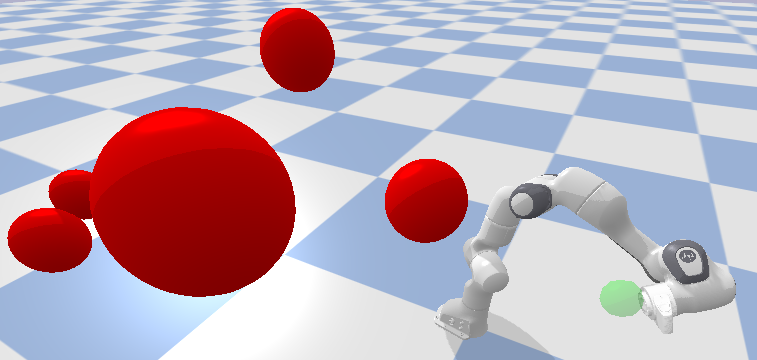
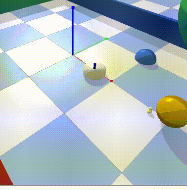
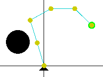
The environment in localPlannerBench is not specific to a single physics simulator and should even be compatible with the real world through e.g. a ROS bridge (modularity). However, at the time of writing, two physics simulators are officially supported (see Fig. 1), planar environments are based on a simple ODE-simulation and pybullet [19] is used for more complex 3D environments. In the pybullet environments we use the unified robot description format (URDF) that allows to import new robots simply by this robot description. To achieve a clean separation between the simulation environment and planning algorithm, we opted to design an Open-AI gym [20] environment wrapper for the different robot types and control modalities that we support (Simplicity, Modularity). Pybullet is not considered the most accurate physics engine, but it is much easier to install compared to competing simulators like ISAAC-Gym [21] or MuJoCo [22] (Simplicity). Besides, as low-level control and interactive motion planning are outside of our scope, the accuracy of PyBullet is considered sufficient (Specificity).

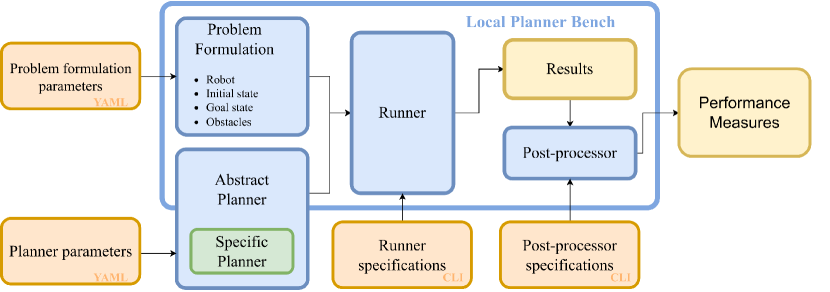
III-E Code structure

The code in localPlannerBench is split up into components as can be seen in Fig. 2. Each component has a unique and clearly defined responsibility (Modularity). The parameters specifying specific configurations of these components are as much as possible defined outside of the code itself using yaml-files. When possible, the code structure reflects the definitions proposed in Section III-B:

•

The Problem class corresponds to the problem formulation and requires its own configuration file to read in the requested problem formulation. Additionally, the component supports randomization of the initial configuration, goal state, and obstacle states. The limits of the randomization should also be defined within the configuration file.
•

The AbstractPlanner is a blueprint for a planner class. When a user creates a new planner, she should derive from this provided base class, so that the planner will automatically be registered as a valid planner to the rest of the package. A planner created using this component is parameterized by the corresponding configuration file.
•

The runner executable is the entry point when running a trial or study i.e. it is the executable that the user interacts with. The component contains the code for the actual execution loops over the Open-AI gym simulation environments and saves the results afterward.
•

The post-processor executable processes the results based on user specified metrics and plot characteristics. Like the runner, it is an executable that the user interacts with.

III-F Usage

There are currently two general possible usages of localPlannerBench: (a) access an open implementation of a local motion planner and its tuned parameters by an expert or (b) compare your own local motion planner against baselines that are already implemented in localPlannerBench

III-G Running a study

localPlannerBench provides a minimal command-line interface (CLI) that processes the configuration files described in the previous section. The CLI calls the runner that runs a study with the given parameters. Specifically, the user specifies the location of the configurations files for the problem formulation and the planner. Additionally, flags and arguments for the study can be speficied through the CLI. For example, the user could specify the location of the output files, whether the simulation should be rendered or not, how many trials should be run, etc. Finally, all relevant information to reproduce a study is saved in a time-stamped results folder. An overview of arguments can be found in Table I.

Argument		Explanation
caseSetup	:	Path to problem formulation file.
planners	:	List of paths to planner configuration files.
res-folder	:	Path to store the result data.
render	:	Display GUI.
numberRuns	:	How many trials to run.
random-goal	:	Should the goal be random?
random-init	:	Should the initial configuration be random?
random-obst	:	Should the obstacles be random?

TABLE I: List of CLI arguments for the runner executable

III-H Postprocessing a study

To promote better reproducibility, running, and post-processing a study is completely separated. Specifically, the output of a study is the raw data that was directly accessible during the execution. That is: the joint position, the joint velocities, the taken actions, the positions of the links of the robot, the position of obstacles, and the goal at each time step. During post-processing, the raw data is evaluated according to user metrics and is potentially plotted. Several performance metrics are implemented, see the repository for a full list. However, additional metrics could be added using a similar approach as for the planner. An overview of post-processor arguments can be found in Table II.

Argument		Explanation
expFolder	:	Path to the results of a study.
kpis	:	List of all kpis/metrics to be evaluated.
plot	:	Auto-generate plot from results.
series	:	Are you evaluating a single trial or multiple?
compare	:	Are you comparing planners?

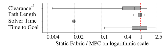
TABLE II: CLI arguments for the post_processor executable

IV EXAMPLE: Optimization fabrics vs MPC

An example of how localPlannerBench can be used to compare the two methods, Static Fabrics and Model Predictive Control (MPC), is found in [4]. The goal of the comparison was to investigate if the significant reduction in solver time of Static Fabrics impacts other metrics like path length, clearance or time to goal. Using the runner, a study was run for a hundred trials, including both planners. Afterwards, the plots in Figure 3 were generated using the post-processor.

V CONCLUSION

As the field of local motion planning matures, the need for standardized reproducible benchmarks increases. To make the life of a researcher a little easier, we’ve created localPlannerBench. This framework is capable of simulating local motion planning problems, for many different robots, modalities, and environments. Furthermore, localPlannerBench is fully open source and designed with simplicity, modularity, and specificacy in mind, enabling users to easily modify localPlannerBench to fit their unique use cases as long as they fit within the scope as what we define as local motion planning. In the future, we hope to extend localPlannerBench in several ways: integrating basic global planning methods to provide reference trajectories for local planning, adding artificial uncertainty to the states and observations to help make the studies more representative of real scenarios, adding support for observations in the form of occupancy maps, semantic maps, or even direct camera or lidar data to accommodate new directions in local motion planning. localPlannerBench has already been proven to be useful for academic comparison and evaluations [4], and we hope it will gain futher attention in this field of local motion planning.

References

[1] K. B. Kaldestad, S. Haddadin et al., “Collision avoidance with potential fields based on parallel processing of 3d-point cloud data on the gpu,” in 2014 IEEE International Conference on Robotics and Automation (ICRA). IEEE, 2014, pp. 3250–3257.
[2] J. Van Den Berg, J. Snape et al., “Reciprocal collision avoidance with acceleration-velocity obstacles,” in 2011 IEEE International Conference on Robotics and Automation. IEEE, 2011, pp. 3475–3482.
[3] N. D. Ratliff, J. Issac et al., “Riemannian motion policies,” arXiv preprint arXiv:1801.02854, 2018.
[4] N. D. Ratliff, K. Van Wyk et al., “Optimization fabrics,” arXiv preprint arXiv:2008.02399, 2020.
[5] M. Spahn, M. Wisse, and J. Alonso-Mora, “Dynamic optimization fabrics for motion generation,” arXiv preprint arXiv:2205.08454, 2022.
[6] M. Kalakrishnan, S. Chitta et al., “Stomp: Stochastic trajectory optimization for motion planning,” in 2011 IEEE international conference on robotics and automation. IEEE, 2011, pp. 4569–4574.
[7] L. Hewing, K. P. Wabersich et al., “Learning-based model predictive control: Toward safe learning in control,” Annual Review of Control, Robotics, and Autonomous Systems, vol. 3, pp. 269–296, 2020.
[8] B. Brito, M. Everett et al., “Where to go next: learning a subgoal recommendation policy for navigation in dynamic environments,” IEEE Robotics and Automation Letters, vol. 6, no. 3, pp. 4616–4623, 2021.
[9] M. Dharmadhikari, T. Dang et al., “Motion primitives-based path planning for fast and agile exploration using aerial robots,” in 2020 IEEE International Conference on Robotics and Automation (ICRA). IEEE, 2020, pp. 179–185.
[10] K. Hauser, T. Bretl et al., “Using motion primitives in probabilistic sample-based planning for humanoid robots,” in Algorithmic foundation of robotics VII. Springer, 2008, pp. 507–522.
[11] C. Wang, Q. Zhang et al., “Learning Mobile Manipulation through Deep Reinforcement Learning,” Sensors, vol. 20, no. 3, p. 939, Feb. 2020. [Online]. Available: https://www.mdpi.com/1424-8220/20/3/939
[12] T. Jurgenson and A. Tamar, “Harnessing Reinforcement Learning for Neural Motion Planning,” in Robotics: Science and Systems XV. Robotics: Science and Systems Foundation, Jun. 2019. [Online]. Available: http://www.roboticsproceedings.org/rss15/p26.pdf
[13] I. A. Șucan, M. Moll, and L. E. Kavraki, “The Open Motion Planning Library,” IEEE Robotics and Automation Magazine, vol. 19, no. 4, pp. 72–82, 12 2012.
[14] D. Coleman, I. Sucan et al., “Reducing the barrier to entry of complex robotic software: a moveit! case study,” arXiv preprint arXiv:1404.3785, 2014.
[15] R. Diankov and J. J. Kuffner, “Openrave: A planning architecture for autonomous robotics,” 2008.
[16] C. Chamzas, C. Quintero-Pena et al., “Motionbenchmaker: A tool to generate and benchmark motion planning datasets,” IEEE Robotics and Automation Letters, vol. 7, no. 2, pp. 882–889, 2021.
[17] L. Kästner, T. Bhuiyan et al., “Arena-bench: A benchmarking suite for obstacle avoidance approaches in highly dynamic environments,” IEEE Robotics and Automation Letters, vol. 7, no. 4, pp. 9477–9484, 2022.
[18] E. Heiden, L. Palmieri et al., “Bench-mr: A motion planning benchmark for wheeled mobile robots,” IEEE Robotics and Automation Letters, vol. 6, no. 3, pp. 4536–4543, 2021.
[19] E. Coumans and Y. Bai, “Pybullet, a python module for physics simulation for games, robotics and machine learning,” http://pybullet.org, 2016–2021.
[20] G. Brockman, V. Cheung et al., “Openai gym,” 2016.
[21] V. Makoviychuk, L. Wawrzyniak et al., “Isaac gym: High performance gpu-based physics simulation for robot learning,” 2021. [Online]. Available: https://arxiv.org/abs/2108.10470
[22] E. Todorov, T. Erez, and Y. Tassa, “Mujoco: A physics engine for model-based control,” in 2012 IEEE/RSJ International Conference on Intelligent Robots and Systems. IEEE, 2012, pp. 5026–5033.