Modular Flows: Differential Molecular Generation

Abstract

Generating new molecules is fundamental to advancing critical applications such as drug discovery and material synthesis. Flows can generate molecules effectively by inverting the encoding process, however, existing flow models either require artifactual dequantization or specific node/edge orderings, lack desiderata such as permutation invariance, or induce discrepancy between the encoding and the decoding steps that necessitates post hoc validity correction. We circumvent these issues with novel continuous normalizing E(3)-equivariant flows, based on a system of node ODEs coupled as a graph PDE, that repeatedly reconcile locally toward globally aligned densities. Our models can be cast as message passing temporal networks, and result in superlative performance on the tasks of density estimation and molecular generation. In particular, our generated samples achieve state of the art on both the standard QM9 and ZINC250K benchmarks.

1 Introduction

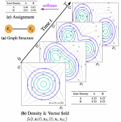
Figure 1: A toy illustration of ModFlow  in action with a two-node graph. The two local flows - $\mathbf{z}_{1}$ and $\mathbf{z}_{2}$ - co-evolve toward a more complex joint density, both driven by the same differential $f$.

Generative models have rapidly become ubiquitous in machine learning with advances from image synthesis (Ramesh et al., 2022) to protein design (Ingraham et al., 2019). Molecular generation (Stokes et al., 2020) has also received significant attention owing to its promise for discovering new drugs and materials. Searching for valid molecules in prohibitively large discrete spaces is, however, challenging: estimates for drug-like structures range between $10^{23}$ and $10^{60}$ but only a tiny fraction - on the order of $10^{8}$ - has been synthesized (Polishchuk et al., 2013; Merz et al., 2020). Thus, learning representations that exploit appropriate molecular inductive biases (e.g., spatial correlations) becomes crucial.

Table 1: A comparison of generative modeling approaches for molecules.

Method	One-shot	Modular	Invertible	Continuous-time
JT-VAE	✓	✓	✗	✗	Jin et al. (2018)
MRNN	✗	✗	✗	✗	Popova et al. (2019)
GraphAF	✗	✗	✓	✗	Shi et al. (2020)
GraphDF	✗	✗	✓	✗	Luo et al. (2021)
MoFlow	✓	✗	✓	✗	Zang and Wang (2020)
GraphNVP	✓	✗	✓	✗	Madhawa et al. (2019)
ModFlow	✓	✓	✓	✓	this work

Earlier models focused on generating sequences based on the SMILES notation (Weininger, 1988) used in Chemistry to describe the molecular structures as strings. However, they were supplanted by generative models that capture valuable spatial information such as bond strengths and dihedral angles, e.g., by embedding molecular graphs via some graph neural network (GNNs) (Scarselli et al., 2009; Garg et al., 2020). Such models primarily include variants of Generative Adversarial Networks (GANs), Variational Autoencoders (VAEs), and Normalizing Flows (Dinh et al., 2014, 2016). Besides known issues with their training, GANs (Goodfellow et al., 2014; Maziarka et al., 2020) suffer from the well-documented problem of mode collapse, thereby generating molecules that lack diversity. VAEs (Kingma and Welling, 2013; Lim et al., 2018; Jin et al., 2018), on the other hand, are susceptible to a distributional shift between the training data and the generated samples. Moreover, optimizing for likelihood via a surrogate lower bound is likely insufficient to capture the complex dependencies inherent in the molecules.

Flows are especially appealing since, in principle, they enable estimating (and sampling from) complex data distributions using a sequence of invertible transformations on samples from a more tractable continuous distribution. Molecules are discrete, so many flow models (Madhawa et al., 2019; Honda et al., 2019; Shi et al., 2020) add noise during encoding and later apply a dequantization procedure. However, dequantization begets distortion and issues related to convergence (Luo et al., 2021). Moroever, many methods segregate the generation of atoms from bonds, so the decoded structure is often not a valid molecule and requires post hoc correction to ensure validity (Zang and Wang, 2020), effecting a discrepancy between the encoding and the decoded distributions. Permutation dependence is another undesirable artifact of these methods. Some alternatives have been explored to avoid dequantization, e.g., (Lippe and Gavves, 2021) encodes molecules in a continuous latent space via variational inference and jointly optimizes a flow model for generation. Discrete graph flows (Luo et al., 2021) also circumvent the many pitfalls of dequantization by resorting to discrete latent variables, and performing validity checks during the generative process. However, discrete flows follow an autoregressive procedure that requires a specific ordering of nodes and edges during training. In general, one shot methods can generate much faster than discrete flows.

We offer a different flow-based perspective tailored to molecules. Specifically, we suggest coupled continuous normalizing E(3)-equivariant flows that bestow generative capabilities from neural partial differential equation (PDE) models on graphs. Graph PDEs have been known to enable designing new embedding methods such as variants of GNNs (Chamberlain et al., 2021), extending GNNs to continuous layers as Neural ODEs (Poli et al., 2019), and accommodating spatial information (Iakovlev et al., 2020). We instead seek to bring to the fore their efficacy and elegance as tools to help generate complex objects, such as molecules, viewed as outcomes resulting from an interplay of co-adapting latent trajectories (i.e., underlying dynamics). Concretely, a flow is associated with each node of the graph, and these flows are conjoined as a joint ODE system conditioned on neighboring nodes. While these flows originate independently as samples from simple distributions, they adjust progressively toward more complex joint distributions as they repeatedly interact with the neighboring flows. We view molecules as samples generated from the globally aligned distributions obtained after many such local feedback iterations. We call the proposed method Modular Flows (ModFlows) to underscore that each node can be regarded as a module that coordinates with other modules. Table 1 summarizes the capabilities of ModFlow compared to some previous generative works.

Contributions.

We propose to learn continuous-time, flow based generative models, grounded on graph PDEs, for generating molecules without resorting to any validity correction. In particular,

• we propose ModFlow, a novel generative model based on coupled continuous normalizing E(3)-equivariant flows. ModFlow  encapsulates essential inductive bias using PDEs, and defines multiple flows that interact locally toward a globally consistent joint density;

• we encode permutation, translation, rotation, and reflection equivariance with E(3) equivariant GNNs adapted to molecular generation, and can leverage 3D geometric information;

• ModFlow  is end-to-end trainable, non-autoregressive, and obviates the need for any external validity checks or correction;

• empirically, ModFlow  achieves state-of-the-art performance on both the standard QM9 (Ramakrishnan et al., 2014) and ZINC250K (Irwin et al., 2012) benchmarks.

Figure 2: A demonstration of the modular flow generation. The initial Gaussian distributions $\mathcal{N}(0,I)$ evolve into complex densities $\mathbf{z}(T)$ under $f$ and are subsequently translated into probabilities and labels.

2 Related works

Generative models.

Earlier attempts for molecule generation (Kusner et al., 2017; Dai et al., 2018) aimed at representing molecules as SMILES strings (Weininger, 1988) and developed sequence generation models. A challenge for these approaches is to learn complicated grammar rules that can generate syntactically valid sequences of molecules. Recently, representing molecules as graphs has inspired new deep generative models for molecular generation (Segler et al., 2018; Samanta et al., 2018; Neil et al., 2018), ranging from VAEs (Jin et al., 2018; Kajino, 2019) to flows (Madhawa et al., 2019; Luo et al., 2021; Shi et al., 2020). The core idea is to learn to encode molecular graphs into a latent space, and subsequently decode samples from this latent space to generate new molecules (Atwood and Towsley, 2016; Xhonneux et al., 2020; You et al., 2018).

Graph partial differential equations.

Graph PDEs is an emerging area that studies PDEs on structured data encoded as graphs. For instance, one can define a PDE on graphs to track the evolution of signals defined over the graph nodes under some dynamics. Graph PDEs have enabled, among others, design of new graph neural networks; see, e.g., works such as GNODE (Poli et al., 2019), NeuralPDE (Iakovlev et al., 2020), Neural operator (Li et al., 2020), GRAND (Chamberlain et al., 2021), and PDE-GCN (Eliasof et al., 2021). Different from all these works, we focus on using PDEs for generative modeling of molecules (as graph-structured objects). Interestingly,  ModFlow  proposed in this work may be viewed as a new equivariant temporal graph network (Rossi et al., 2020; Souza et al., 2022).

Validity oracles.

A key challenge of molecular generative models is to be able to generate valid molecules, according to various criteria for molecular validity or feasibility. It is a common practice to call on external chemical software as rejection oracles to reduce or exclude invalid molecules, or do validity checks as part of autoregressive generation (Luo et al., 2021; Shi et al., 2020; Popova et al., 2019). An important open question has been whether generative models can learn to achieve high generative validity intrinsically, i.e., without being aided by oracles or resorting to additional checks.  ModFlow  takes a major step forward toward that goal.

3 Modular Flows

We focus on unsupervised learning of an underlying graph density $p(G)$ using a dataset of observed molecular graphs $\mathcal{D}=\{G_{n}\}_{n=1}^{N}$. We learn a generative flow model $p_{\theta}(G)$ specified by flow parameters $\theta$, and use it to sample novel high-probability molecules.

3.1 Molecular Representation

Graph representation.

We represent each molecular graph $G=(V,E)$ of size $M$ as a tuple of vertices $V=(v_{1},\ldots,v_{M})$ and edges $E\subset V\times V$. Each vertex takes a value from an alphabet on atoms: $v\in\mathcal{A}=\{\texttt{C},\texttt{H},\texttt{N},\texttt{O},\texttt{P},\texttt{S},\ldots\}$; while each edge $e\in\mathcal{B}=\{1,2,3\}$ abstracts some bond type (i.e., single, double, or triple). We assume that, conditioned on the edges, the graph likelihood factorizes as a product of categorical distributions over vertices given their latent representations:

$$p(G) :=p(V|E,\{z\})=\prod_{i=1}^{M}\operatorname*{Cat}(v_{i}|\sigma(\mathbf{z}_{i}))~{},$$ (1)

where $\mathbf{z}_{i}=(z_{i\texttt{C}},z_{i\texttt{H}},\ldots)\in\mathbb{R}^{|\mathcal{A}|}$ is a set of atom scores for node $i$ such that $z_{ik}\in\mathbb{R}$ pertains to type $k\in\mathcal{A}$, and $\sigma$ is the softmax function

$$\sigma(\mathbf{z}_{i})_{k} =\frac{\exp(\mathbf{z}_{ik})}{\sum_{k^{\prime}}\exp(\mathbf{z}_{ik^{\prime}})}~{},$$ (2)

which turns the real-valued scores $\mathbf{z}_{i}$ into normalized probabilities.  ModFlow  also supports 3D molecular graphs that contain atomic coordinates and angles as additional information.

Tree representations.

We can obtain an alternative representation for molecules: we can decompose each molecule into a tree-like structure, by contracting certain vertices into a single node (denoted as a cluster) such that the molecular graph becomes acyclic. Following Jin et al. (2018), we restrict these clusters to ring substructures present in the molecular data, in addition to the atom alphabet. Thus, we obtain an extended alphabet $\mathcal{A}_{\mathrm{tree}}=\mathcal{A}\cup\{\texttt{C}_{1},\texttt{C}_{2},\ldots\}$, where each cluster label $\texttt{C}_{r}$ corresponds to some ring substructure in the label vocabulary $\textstyle\chi$. We then reduce the vocabulary to the $30$ most commonly occurring substructures of $\mathcal{A}_{\mathrm{tree}}$. For further details, see Appendix A.2.

3.2 Differential modular flows

Normalizing flows (Kobyzev et al., 2021) provide a general recipe for constructing flexible probability distributions, used in density estimation (Cramer et al., 2021; Huang et al., 2018) and generative modeling (Zhen et al., 2020; Zang and Wang, 2020). We propose to model the atom scores $\mathbf{z}_{i}(t)$ as a Continuous-time Normalizing Flow (CNF) (Grathwohl et al., 2018) over time $t\in\mathbb{R}_{+}$. We assume the initial scores at time $t=0$ follow an uninformative Gaussian base distribution $\mathbf{z}_{i}(0)\sim\mathcal{N}(0,I)$ for each node $i$. Node scores evolve in parallel over time according to the differential equation

$$\dot{\mathbf{z}}_{i}(t) :=\frac{\partial\mathbf{z}_{i}(t)}{\partial t}=f_{\theta}\big{(}t,\mathbf{z}_{i}(t),\mathbf{z}_{\mathcal{N}_{i}}(t),\mathbf{x}_{i},\mathbf{x}_{\mathcal{N}_{i}}\big{)},\qquad i\in\{1,\ldots,M\}~{},$$ (3)

where $\mathcal{N}_{i}=\{j:(i,j)\in E\}$ is the set of neighbors of node $i$ and $\mathbf{z}_{\mathcal{N}_{i}}(t)=\{\mathbf{z}_{j}(t):j\in\mathcal{N}_{i}\}$ the scores of the neighbors at time $t$; $\mathbf{x}_{i}$ and $\mathbf{x}_{\mathcal{N}_{i}}$ denote, respectively, the positional (2D/3D) information of $i$ and its neighbours; and $\theta$ denotes the parameters of the flow function $f$ to be learned. Stacking together all node differentials, we obtain a modular system of coupled ODEs:

$$\dot{\mathbf{z}}(t) =\begin{pmatrix}\dot{\mathbf{z}}_{1}(t)\\ \vdots\\ \dot{\mathbf{z}}_{M}(t)\end{pmatrix}=\begin{pmatrix}f_{\theta}\big{(}t,\mathbf{z}_{1}(t),\mathbf{z}_{\mathcal{N}_{1}}(t),\mathbf{x}_{i},\mathbf{x}_{\mathcal{N}_{i}}\big{)}\\ \vdots\\ f_{\theta}\big{(}t,\mathbf{z}_{M}(t),\mathbf{z}_{\mathcal{N}_{M}}(t),\mathbf{x}_{i},\mathbf{x}_{\mathcal{N}_{i}}\big{)}\end{pmatrix}$$ (4)

$$\mathbf{z}(T) =\mathbf{z}(0)+\int_{0}^{T}\dot{\mathbf{z}}(t)dt~{}.$$ (5)

This coupled system of ODEs may be viewed as a graph PDE (Iakovlev et al., 2020; Chamberlain et al., 2021), where the evolution of each node depends only on its neighbors.

The joint flow induces a corresponding change in the individual densities in terms of divergence of $f$ (Chen et al., 2018),

$$\frac{d\log p_{t}(\mathbf{z}_{i}(t))}{dt} =-\operatorname*{tr}\left(\frac{\partial f_{\theta}\big{(}t,\mathbf{z}_{i}(t),\mathbf{z}_{\mathcal{N}_{i}}(t),\mathbf{x}_{i},\mathbf{x}_{\mathcal{N}_{i}}\big{)}}{\partial\mathbf{z}_{i}}\right),$$ (6)

starting from the base distribution $p_{0}(\mathbf{z}_{i}(0))=\mathcal{N}(\mathbf{z}_{i}(0)|0,I)$. The trace picks only the diagonal elements of the Jacobian $\frac{\partial f}{\partial\mathbf{z}}$, which interprets the input from neighbors, $\mathbf{z}_{\mathcal{N}_{i}}$, as a ‘control’ for each node $\mathbf{z}_{i}$ at each instant $t$. An ODE solver is used for such systems, and the gradients are computed via the adjoint sensitivity method (Kolmogorov et al., 1962). This approach incurs a low memory cost, and explicitly controls the numerical error. Notably, moving towards modular flows translates sparsity also to the adjoints.

Proposition 1:

Modular adjoints are sparser than regular adjoints. They can be computed as

$$\frac{d\bm{\lambda}_{i}}{dt} =-\bm{\lambda}(t)^{\top}\frac{\partial f\big{(}t,\mathbf{z}_{i}(t),\mathbf{z}_{\mathcal{N}_{i}}(t),\mathbf{x}_{i},\mathbf{x}_{\mathcal{N}_{i}}\big{)}}{\partial\mathbf{z}}=-\sum_{j\in\mathcal{N}_{i}\cup\{i\}}\bm{\lambda}_{j}(t)^{\top}\frac{\partial f\big{(}t,\mathbf{z}_{i}(t),\mathbf{z}_{\mathcal{N}_{i}}(t),\mathbf{x}_{i},\mathbf{x}_{\mathcal{N}_{i}}\big{)}}{\partial\mathbf{z}_{j}},$$ (7)

where the partial derivatives $\frac{\partial f}{\partial\mathbf{z}}=[\frac{\partial f_{i}}{\partial\mathbf{z}_{j}}]_{ij}$ are sparse (see Appendix A.1 for the derivation).

3.3 Equivariant local differential

Our goal is to have a differential function $f$ that is a PDE operator used in  Equation 4, and that satisfies the natural equivariances and invariances of the molecules. Specifically, this function must be (i) translation equivariant: translating the input results in an equivalent translation of the output; (ii) rotational (and reflection) equivariant: rotating the input results in an equivalent rotation of the output; and (iii) permutation equivariant: permuting the input results in the same permutation of the output. Therefore, we chose to use E(3)-Equivariant GNN (EGNN)  (Satorras et al., 2021), which is translation, rotation and reflection equivariant (E(n)), and permutation equivariant with respect to an input set of points (see Appendix A.3 for details). EGNN takes as input the node embeddings as well as the geometric information (polar coordinates (2D) and spherical polar coordinates (3D)). Interestingly, ModFlow  can be viewed as a message passing temporal graph network (Rossi et al., 2020; Souza et al., 2022) as shown next.

Proposition 2:

Modular Flows can be cast as message passing Temporal Graph Networks (TGNs). The operations are listed in Table 2, where ModFlow  is subjected to a single layer of EGNN. (See Appendix A.4 for more details).

Table 2: ModFlow  as a temporal graph network (TGN). Adopting notation for TGNs from Rossi et al. (2020) $v_{i}$ is a node-wise event on $i$; $e_{ij}$ denotes an (asymmetric) interaction between $i$ and $j$; $\mathbf{s}_{i}$ is the memory of node $i$; and $t$ and $t^{-}$ denote time with $t^{-}$ being the time of last interaction before $t$, e.g., $\mathbf{s}_{i}(t^{-})$ is the memory of $i$ just before time $t$; and $\operatorname{msg}$ and $\operatorname{agg}$ are learnable functions (e.g., MLP) to compute, respectively, the individual and the aggregate messages. For ModFlow, we use $\mathbf{r}_{ij}$ to denote the spatial distance $\mathbf{x}_{i}-\mathbf{x}_{j}$, and $a_{ij}$ to denote the attributes of the edge between $i$ and $j$. The functions $\phi_{e}$, $\phi_{x}$, and $\phi_{h}$ are as defined in (Satorras et al., 2021).

Method	TGN layer	ModFlow
Edge	$\mathbf{m}_{ij}^{\prime}(t)=\operatorname{msg}\left(\mathbf{s}_{i}\left(t^{-}\right),\mathbf{s}_{j}\left(t^{-}\right),\Delta t,\mathbf{e}_{ij}(t)\right)$	$\mathbf{m}_{ij}(t)=\phi_{e}\left(\mathbf{z}_{i}(t),\mathbf{z}_{j}(t),\left\|\mathbf{r}_{ij}(t)\right\|^{2},a_{ij}\right)$
	$\overline{\mathbf{m}}_{i}^{\prime}(t)=\operatorname{agg}\left(\{\mathbf{m}_{ij}^{\prime}\left(t\right)|j\in\mathcal{N}_{i}\}\right)$	$\mathbf{m}_{i}(t)=\sum_{j\in\mathcal{N}(i)}\mathbf{m}_{ij}$
		$\hat{\mathbf{m}}_{ij}(t)=\mathbf{r}_{ij}(t)\cdot\phi_{x}\left(\mathbf{m}_{ij}(t)\right)$
		$\hat{\mathbf{m}}_{i}(t)=C\sum_{j\in\mathcal{N}(i)}\hat{\mathbf{m}}_{ij}(t)$
Memory state	$\mathbf{s}_{i}(t)=\operatorname{mem}\left(\overline{\mathbf{m}}_{i}^{\prime}(t),\mathbf{s}_{i}\left(t^{-}\right)\right)$	$\mathbf{x}_{i}(t+1)=\mathbf{x}_{i}(t)+\hat{\mathbf{m}}_{i}(t)$
Node	$\mathbf{z}_{i}^{\prime}(t)=\sum_{j\in\mathcal{N}_{i}}h\left(\mathbf{s}_{i}(t),\mathbf{s}_{j}(t),\mathbf{e}_{ij}(t),\mathbf{v}_{i}(t),\mathbf{v}_{j}(t)\right)$	$\mathbf{z}_{i}(t+1)=\phi_{h}\left(\mathbf{z}_{i}(t),\mathbf{m}_{i}(t)\right)$

3.4 Training objective

Normalizing flows are predominantly trained to minimize $\operatorname*{KL}[p_{\mathrm{data}}||p_{\theta}]$, i.e., the KL-divergence between the unknown data distribution $p_{\mathrm{data}}$ and the flow-generated distribution $p_{\theta}$. This objective is equivalent to maximizing $\mathbb{E}_{p_{\mathrm{data}}}[\log p_{\theta}]$ (Papamakarios et al., 2021). However, note that the discrete graphs $G$ and the continuous atom scores $\mathbf{z}(t)$ reside in different spaces. Thus, in order to apply flows, a mapping between the observation space and the flow space is needed. Earlier approaches use dequantisation to turn a graph $G$ into a distribution of latent states, and argmax to deterministically map latent states to graphs (Zang and Wang, 2020).

Figure 3: Plate diagram showing both the inference and generative components of ModFlow.

We instead reduce the learning problem to maximizing $\mathbb{E}_{\hat{p}_{\mathrm{data}}(\mathbf{z}(T))}[\log p_{\theta}(\mathbf{z}(T))]$, where we turn the observed set of graphs $\{G_{n}\}$ into a set of scores $\{\mathbf{z}_{n}\}$ using

$$\mathbf{z}_{n}(G_{n};\epsilon)=(1-\epsilon)~{}\mathrm{onehot}(G_{n})~{}+~{}\dfrac{\epsilon}{|\mathcal{A_{s}}|}\textbf{1}_{M(n)}\textbf{1}_{|\mathcal{A_{s}}|}^{\top}~{},$$

where $\mathrm{onehot}(G_{n})$ is a matrix of size $M(n)\times|\mathcal{A_{s}}|$ (i.e., rows equal to the number of nodes in $G_{n}$ and columns equal to the number of possible node labels) such that $G_{n}(i,k)$ = 1 if $v_{i}=a_{k}\in\mathcal{A_{s}}$, that is if the vertex $i$ is labeled with atom $k$, and 0 otherwise; $\textbf{1}_{q}$ is a vector with $q$ entries each set to 1; $\mathcal{A_{s}}\in\{\mathcal{A},\mathcal{A}_{\rm tree}\}$; and $\epsilon\in[0,1]$ is added to model the noise in estimating the posterior $p({\mathbf{z}(T)|G})$ due to short-circuiting the inference process from $G$ to $\mathbf{z}(T)$ skipping the intermediate dependencies, thereby inducing an unconditional distribution $\hat{p}_{\mathrm{data}}$ that is slightly different from the true data distribution $p_{\mathrm{data}}$. The plate diagram in Figure 3 summarizes the overall procedure.

Effectively, we exploit the (non-reversible) composition of the argmax and softmax operations to transition from the continuous flow space to the discrete graph space, but skip this composition altogether in the reverse direction. Importantly, this short-circuiting allows ModFlow  to keep the forward and backward flows between $\mathbf{z}(0)$ and $\mathbf{z}(T)$ completely aligned (i.e., reversible) unlike previous approaches. We maximize the following objective over $N$ training graphs:

$$\arg\!\max_{\theta}\mathcal{L} =\mathbb{E}_{\hat{p}_{\mathrm{data}}(\mathbf{z})}\log p_{\theta}(\mathbf{z})$$ (8)

$$\approx\frac{1}{N}\sum_{n=1}^{N}\log p_{T}\big{(}\mathbf{z}(T)=\mathbf{z}_{n}\big{)}$$ (9)

$$=\frac{1}{N}\sum_{n=1}^{N}\left(\sum_{i=1}^{M(n)}\log p_{0}(\mathbf{z}_{i}(0))-\sum_{i=1}^{M(n)}\int_{0}^{T}\mathrm{tr}\frac{\partial f_{\theta}(t,\mathbf{z}_{i}(t),\mathbf{z}_{\mathcal{N}_{i}}(t),\mathbf{x}_{i},\mathbf{x}_{\mathcal{N}_{i}})}{\partial\mathbf{z}_{i}(t)}dt\right)~{},$$ (10)

which factorizes over the size $M(n)$ of the $n$’th training molecule. The encoding probability follows from Equation 6, where $\mathbf{z}(0)$ can be traced by traversing the flow $f$ backward in time starting from $\mathbf{z}_{n}$ at time $t=T$ until $t=0$. In practice we solve ODE integrals using a numerical solver such as Runge-Kutta. We thus delegate this task to a general solver of the form $\texttt{ODESolve}(\mathbf{z},f_{\theta},T)$, where map $f_{\theta}$ is applied for $T$ steps starting with $\mathbf{z}$. An optimizer optim is also required for updating $\theta$.

3.5 Molecular generation

Given a molecular structure, we can generate novel molecules by sampling an initial state $\mathbf{z}(0)\sim\mathcal{N}(0,I)$, and running the modular flow forward in time for $T$ steps and obtain $\mathbf{z}(T)$. This procedure maps a tractable base distribution $p_{0}$ to a more complex distribution $p_{T}$. We follow argmax to pick the most probable label assignment for each node (Zang and Wang, 2020). We outline the procedures for training and generation in Algorithm 1 and Algorithm 2 respectively.

Algorithm 1 Training ModFlow

1:Dataset $\mathcal{D}$, iterations $n_{\mathrm{iter}}$, batch size $B$, number of batches $n_{B}$

2:Initialise parameters $\theta$ of ModFlow  (EGNN)

3:for $k=1,\ldots,n_{\mathrm{iter}}$ do

4:   for $b=1,\ldots,n_{B}$ do

5:      Sample $\mathcal{D}_{b}=\{G_{1},\ldots,G_{B}\}$ from $\mathcal{D}$

6:      Define $\mathbf{z}_{b}(T):=\{\mathbf{z}_{r}(T):G_{r}\in\mathcal{D}_{b}\}$

7:      Set $\mathbf{z}_{b}(T)$ to $\mathbf{z}_{b}(G_{b};\epsilon)$

8:      $\mathcal{L}_{b}=\dfrac{1}{B}\displaystyle\sum_{G_{r}\in D_{b}}\log p_{\theta}(\mathbf{z}_{r}(T))$, using         $\mathbf{z}_{b}(0)=\texttt{ODESolve}(\mathbf{z}_{b}(T),f_{\theta}^{-1},T)$

9:   end for

10:   $\theta\xleftarrow{}\texttt{optim}(\frac{1}{n_{B}}\sum_{b=1}^{n_{B}}\mathcal{L}_{b};\theta)$

11:end for

Algorithm 2 Generating with ModFlow

1:Sample $\mathbf{z}(0)\sim\mathcal{N}(0,I)$

2:$\mathbf{z}(T)=\texttt{ODESolve}(\mathbf{z}(0),f_{\theta},T)$

3:Assign labels by $\mathrm{argmax}(\sigma(\mathbf{z}(T)))$

4 Experiments

We first demonstrate the ability of Modular Flows (ModFlow) to learn highly discontinuous synthetic patterns on 2D grids. We also evaluated ModFlow  models trained, variously, on (i) 2D coordinates, (ii) 3D coordinates, (iii) 2D coordinates + tree representation, and (iv) 3D coordinates + tree representation on the tasks of molecular generation and optimization. Our results show that ModFlow  compares favorably to other prominent flow and non-flow based molecular generative models, including GraphDF (Luo et al., 2021), GraphNVP (Madhawa et al., 2019), MRNN(Popova et al., 2019), and GraphAF (Shi et al., 2020). Notably, ModFlow  achieves state-of-the-art results without validity checks or post hoc correction. We also provide results of our ablation studies to underscore the relevance of geometric features and equivariance toward this superlative empirical performance.

4.1 Density Estimation

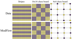
Figure 4: ModFlow  can accurately learn to reproduce complex, discontinuous graph patterns.

We generated our synthetic data in the following way. We considered two variants of a chessboard pattern, namely, (i) $4\times 4$ grid where every node takes a binary value, 0 or 1, and neighboring nodes have different values; and (ii) $16\times 16$ grid where nodes in each block of $4\times 4$ all take the same value (0 or 1), different from the adjacent blocks. We also experimented with a $20\times 20$ grid describing alternating stripes of $0$s and $1$s.

Figure 4 shows that ModFlow  can learn neural differential functions $f_{\theta}$ that reproduce the patterns almost perfectly, indicating sufficient capacity to model complex patterns. That is, ModFlow  is able to transform the initial Gaussian distribution into different multi-modal and discontinuous distributions.

4.2 Molecule Generation

Data.

We trained and evaluated all the models on ZINC250k (Irwin et al., 2012) and QM9 (Ramakrishnan et al., 2014) datasets. The ZINC250k set contains 250,000 drug-like molecules, each consisting of up to 38 atoms. The QM9 set contains 134,000 stable small organic molecules with atoms from the set $\{\texttt{C},\texttt{H},\texttt{O},\texttt{N},\texttt{F}\}$. The molecules are processed to be in the kekulized form with hydrogens removed by the RDkit software (Landrum et al., 2013).

Table 3: Random generation on QM9 (top) and ZINC250K (bottom) without post hoc validity corrections. Results with ^∗ are taken from Luo et al. (2021). Higher values are better for all columns.

Method	Validity %	Uniqueness %	Novelty %	Reconstruction %
GVAE	60.2	9.3	80.9	96.0
GraphNVP∗	83.1	99.2	58.2	100
GRF∗	84.5	66	58.6	100
GraphAF∗	67	94.2	88.8	100
GraphDF∗	82.7	97.6	98.1	100
MoFlow∗	89.0	98.5	96.4	100
ModFlow  (2D-EGNN)	$\textbf{96.2}\pm 1.7$	99.5	100	100
ModFlow  (3D-EGNN)	$\textbf{98.3}\pm 0.7$	99.1	100	100
ModFlow  (JT-2D-EGNN)	$\textbf{97.9}\pm 1.2$	99.2	100	100
ModFlow  (JT-3D-EGNN)	$\textbf{99.1}\pm 0.8$	99.3	100	100

Method	Validity %	Uniqueness %	Novelty %	Reconstruction %
MRNN	65	99.89	100	n/a
GVAE	7.2	9	100	53.7
GCPN	20	99.97	100	n/a
GraphNVP∗	42.6	94.8	100	100
GRF∗	73.4	53.7	100	100
GraphAF∗	68	99.1	100	100
GraphDF∗	89	99.2	100	100
MoFlow∗	50.3	99.9	100	100
ModFlow  (2D-EGNN)	$\textbf{94.8}\pm 1.0$	99.4	100	100
ModFlow  (3D-EGNN)	$\textbf{95.4}\pm 1.2$	99.7	100	100
ModFlow  (JT-2D-EGNN)	$\textbf{97.4}\pm 1.4$	99.1	100	100
ModFlow  (JT-3D-EGNN)	$\textbf{98.1}\pm 0.9$	99.3	100	100

Setup.

We adopt common quality metrics to evaluate molecular generation. Validity is the fraction of molecules that satisfy the respective chemical valency of each atom. Uniqueness refers to the fraction of generated molecules that is unique (i.e, not a duplicate of some other generated molecule). Novelty is the fraction of generated molecules that is not present in the training data. Reconstruction is the fraction of molecules that can be reconstructed from their encoding. Here, we strictly limit ourselves to comparing all methods on their validity scores without resorting to external correction. We trained each model with 5 random weight initializations, and generated 50,000 molecular graphs for evaluation. We report the mean and the standard deviation scores across these multiple runs.

Implementation. The models were implemented in PyTorch (Paszke et al., 2019). The EGNN method used only a single layer with embedding dimension of 32. We trained with the Adam optimizer (Kingma and Ba, 2014) for 50-100 epochs (until the training loss became stable), with batch size 1000 and learning rate $0.001$. ModFlow  is significantly faster compared to autoregressive models such as GraphAF and GraphDF. For more details, see Appendix A.5.

Results. Table 3 reports the performance on QM9 (top) and ZINC250K (bottom) respectively. ModFlow  achieves state-of-the-art results across all metrics. Notably, its reconstruction rate is 100% (similar to other flow models); in addition, however, the novelty (100%) and uniqueness scores ($\approx$99%) are also very high. Moreover, ModFlow  surpassed the other methods on validity (95%-99%).

In Appendix A.6, we document additional evaluations with respect to the MOSES metrics that access the overall quality of generated molecules, as well as the distributions of chemical properties. All these results substantiate the promise of ModFlow  as an effective tool for molecular generation.

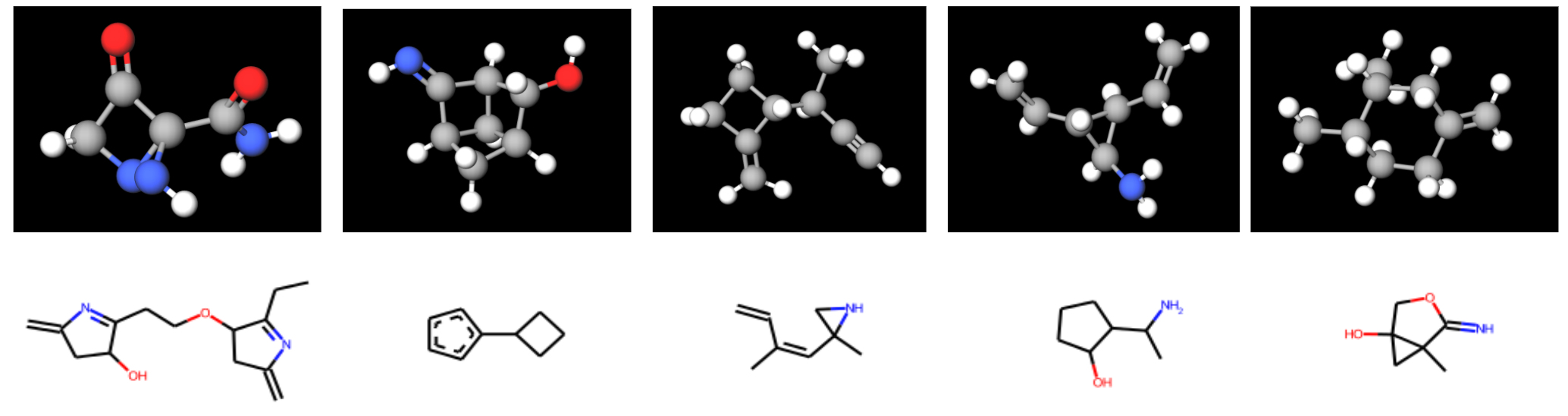
(a) QM9 Dataset

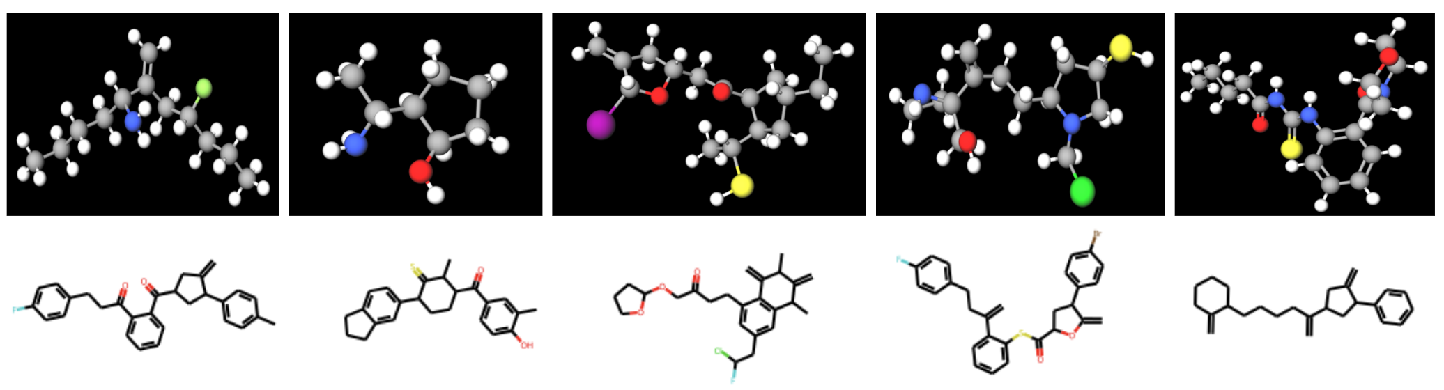
(b) ZINC250K Dataset

Figure 5: Samples of molecules generated by ModFlow. More examples are shown in Appendix A.7.

4.3 Property-targeted Molecular Optimization

The task of molecular optimization is to search for molecules that have better chemical properties. We choose the standard quantitative estimate of drug-likeness (QED) as our target chemical property. QED measures the potential of a molecule to be characterized as a drug. We used a pre-trained ModFlow model $f$ to encode molecules $\mathcal{M}$ into their embeddings $\mathcal{Z}=f(\mathcal{M})$, and applied linear regression to obtain QED scores $\mathcal{Y}$ from these embeddings. We then interpolate in the latent space of each molecule along the direction of increasing QED via several gradient ascent steps, i.e., updates of the form $\mathcal{Z}^{\prime}=\mathcal{Z}+\lambda*\frac{d\mathcal{Y}}{d\mathcal{Z}}$, where $\lambda$ denotes the length of the search step. The final embedding thus obtained is decoded as a new molecule via the reverse mapping $f^{-1}$.

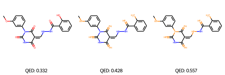
Figure 6: Example of chemical property optimization on the ZINC250K dataset. Given the left-most molecule, we interpolate in latent space along the direction which maximizes its QED property.

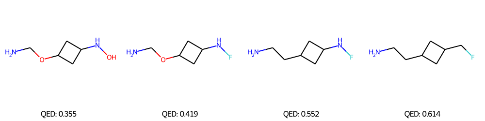
Figure 7: Example of chemical property optimization on the QM9 dataset. Given the left-most molecule, we interpolate in latent space along the direction which maximizes its QED property.

Table 4: Performance in terms of the best QED scores (baselines are taken from Luo et al. (2021)).

Method	1st	2nd	3rd
ZINC (dataset)	0.948	0.948	0.948
JTVAE	0.925	0.911	0.910
GCPN	0.948	0.947	0.945
MRNN	0.844	0.799	0.736
GraphAF	0.948	0.948	0.947
GraphDF	0.948	0.948	0.948
MoFlow	0.948	0.948	0.948
ModFlow  (2D-EGNN)	0.948	0.941	0.937
ModFlow  (3D-EGNN)	0.948	0.937	0.931
ModFlow  (JT-2D-EGNN)	0.947	0.941	0.939
ModFlow  (JT-3D-EGNN)	0.948	0.948	0.945

Figure 6 and Figure 7 show examples of the molecules decoded from the learned latent space using this procedure, starting with molecules having a low QED score. Note that the number of valid molecules decoded back varies on the query molecule. We report the discovered novel molecules sorted by their QED scores in Table 4. Clearly, ModFlow  is able to find novel molecules with high QED scores.

4.4 Ablation Studies

We also performed ablation experiments to gain further insights about ModFlow, as we describe next.

E(3)-equivariant versus not equivariant.

Molecules exhibit translational and rotational symmetries, so we conducted an ablation study to quantify the effect of incorporating these symmetries in our model. We compare the results obtained using an EGNN with a non-equivariant graph convolutional network (GCN). For our purpose, we used a 3-layer GCN with layer sizes 64-32-32. The validity scores in Table 5 provide strong evidence in favor of modeling the symmetries explicitly in the proposed Modular Flows.

Table 5: Random generation performance on ZINC250K and QM9 dataset with E(3)-EGNN vs GCN.

Dataset	Method	Validity %	Uniqueness %	Novelty %
ZINC250K	ModFlow (3D-EGNN)	$95.4\pm 1.2$	99.7	100
	ModFlow (GCN)	$90.3\pm 1.9$	99.7	100
QM9	ModFlow (3D-EGNN)	$98.3\pm 0.7$	99.1	100
	ModFlow (GCN)	$93.3\pm 0.5$	98.8	100

2D versus 3D.

Finally, we study whether including information about the 3D coordinates improves the model. Note that the EGNN-coupled differential function obtains either the 2D or 3D positions as polar coordinates, where the 3D positions have an extra degree of freedom. Table 6 shows that transitioning from 2D to 3D improves the mean validity score.

Table 6: Random generation on ZINC250K and QM9 dataset with 2D versus 3D features.

Dataset	Method	Validity %	Uniqueness %	Novelty %
ZINC250K	ModFlow (3D-EGNN)	$95.4\pm 1.2$	99.7	100
	ModFlow (2D-EGNN)	$94.8\pm 1.0$	99.4	100
QM9	ModFlow (3D-EGNN)	$98.3\pm 0.7$	99.1	100
	ModFlow (2D-EGNN)	$96.2\pm 1.7$	99.5	100

5 Conclusion

We proposed ModFlow, a new generative flow model where multiple flows interact locally according to a coupled ODE, resulting in accurate modeling of graph densities and high quality molecular generation without any validity checks or correction. Interesting avenues open up, including the design of (a) more nuanced mappings between discrete and continuous spaces, and (b) extensions of modular flows to (semi-)supervised settings.

6 Acknowledgments

The calculations were performed using resources within the Aalto University Science-IT project. This work has been supported by the Academy of Finland under the HEALED project (grant 13342077).

Appendix A Appendix

A.1 Derivation of modular adjoint

We present a standard adjoint gradient derivation (Bradley, 2019), and show that the adjoint of a graph neighborhood differential is sparse.

For completeness, we define an ODE system

$$\dot{\mathbf{z}}(t) =f(\mathbf{z},t,{\bm{\theta}})$$ (11)

$$\mathbf{z}(t) =\mathbf{z}_{0}+\int_{0}^{t}f(\mathbf{z},t,{\bm{\theta}})d\tau,$$ (12)

where $\mathbf{z}\in\mathbb{R}^{D}$ is a state vector, $\dot{\mathbf{z}}\in\mathbb{R}^{D}$ is the state time differential defined by the vector field function $f$ and parameterised by ${\bm{\theta}}$. The starting state is $\mathbf{z}_{0}$, and $t,\tau\in\mathbb{R}_{+}$ are time variables. Our goal is to solve a constrained problem

$$\min_{\bm{\theta}}\qquad G({\bm{\theta}})=\int_{0}^{T}g(\mathbf{z},t,{\bm{\theta}})dt$$ (13)

$$s.t.\qquad \dot{\mathbf{z}}-f(\mathbf{z},t,{\bm{\theta}})=0,\qquad\forall t\in[0,T]$$ (14)

$$\mathbf{z}(0)-\mathbf{z}_{0}=0,$$ (15)

where $G$ is the total loss that consists of instant loss functionals $g$. We desire to compute the gradients of the system $\nabla_{\bm{\theta}}G$.

We optimise the constrained problem by solving the Lagrangian

$$\mathcal{L}({\bm{\theta}},\bm{\lambda},\bm{\mu}) =G({\bm{\theta}})+\int_{0}^{T}\bm{\lambda}(t)^{\top}(\dot{\mathbf{z}}-f(\mathbf{z},t,{\bm{\theta}}))dt+\bm{\mu}^{\top}(\mathbf{z}(0)-\mathbf{z}_{0})$$ (16)

$$=\int_{0}^{T}\Big{[}g(\mathbf{z},t,{\bm{\theta}})+\bm{\lambda}(t)^{\top}(\dot{\mathbf{z}}-f(\mathbf{z},t,{\bm{\theta}}))\Big{]}dt+\bm{\mu}^{\top}(\mathbf{z}(0)-\mathbf{z}_{0})~{}.$$ (17)

The constraints are satisfied by the ODE definition. Hence, $\nabla_{\bm{\theta}}\mathcal{L}=\nabla_{\bm{\theta}}G$, and we can set values ${\bm{\theta}}$ and $\bm{\mu}$ freely. We use a shorthand notation $\frac{\partial a}{\partial b}=a_{b}$, and omit parameters from the functions for notational simplicity. Applying the chain rule, we note that the gradient becomes

$$\nabla_{\bm{\theta}}\mathcal{L} =\nabla_{\bm{\theta}}G=\int_{0}^{T}\Big{[}\color[rgb]{0,0,0}g_{\mathbf{z}}\mathbf{z}_{\bm{\theta}}+g_{\bm{\theta}}+\bm{\lambda}^{\top}\dot{\mathbf{z}}_{\bm{\theta}}-\bm{\lambda}^{\top}f_{\mathbf{z}}\mathbf{z}_{\bm{\theta}}-\bm{\lambda}^{\top}f_{\bm{\theta}}\Big{]}\color[rgb]{0,0,0}dt~{},$$ (18)

where the $\bm{\mu}$ term drops out since it does not depend on parameters ${\bm{\theta}}$. We apply integration by parts to swap the differentials in term $\bm{\lambda}^{\top}\dot{\mathbf{z}}_{\bm{\theta}}$, resulting in

$$\int_{0}^{T}\bm{\lambda}^{\top}\dot{\mathbf{z}}_{\bm{\theta}}dt =\bm{\lambda}^{\top}\mathbf{z}_{\bm{\theta}}|_{t=T}-\bm{\lambda}^{\top}\mathbf{z}_{\bm{\theta}}|_{t=0}-\int_{0}^{T}\dot{\bm{\lambda}}^{\top}\mathbf{z}_{\bm{\theta}}dt~{}.$$ (19)

Substituting this into previous equation and rearranging the terms results in

$$\nabla_{\bm{\theta}}\mathcal{L} =\int_{0}^{T}\underbrace{(g_{\mathbf{z}}-\bm{\lambda}^{\top}f_{\mathbf{z}}-\dot{\bm{\lambda}}^{\top})\mathbf{z}_{\bm{\theta}}}_{0,\text{ if }\dot{\bm{\lambda}}^{\top}=g_{\mathbf{z}}-\bm{\lambda}^{\top}f_{\mathbf{z}}}dt+\int_{0}^{T}(g_{\bm{\theta}}-\bm{\lambda}^{\top}f_{\bm{\theta}})dt+\underbrace{\bm{\lambda}^{\top}\mathbf{z}_{\bm{\theta}}|_{t=T}}_{0,\text{ if }\bm{\lambda}(T)=\mathbf{0}}-\underbrace{\bm{\lambda}^{\top}\mathbf{z}_{\bm{\theta}}|_{t=0}}_{0}.$$ (20)

The last term is removed since $\mathbf{z}(0)$ not depend on ${\bm{\theta}}$ as a constant, and thus $\mathbf{z}_{\bm{\theta}}(0)=0$. The difficult term in the equation is $\mathbf{z}_{\bm{\theta}}$. We remove it by choosing

$$\dot{\bm{\lambda}}^{\top} =g_{\mathbf{z}}-\bm{\lambda}^{\top}f_{\mathbf{z}}.$$ (21)

Finally, we choose $\bm{\lambda}(T)=0$ which also removes the second-to-last term. The choices lead to a final term

$$\nabla_{\bm{\theta}}G=\nabla_{\bm{\theta}}\mathcal{L} =\int_{0}^{T}(\color[rgb]{0,0,0}g_{\bm{\theta}}-\bm{\lambda}^{\top}f_{\bm{\theta}})\color[rgb]{0,0,0}dt$$ (22)

$$s.t.\quad \dot{\bm{\lambda}}^{\top}=g_{\mathbf{z}}-\bm{\lambda}^{\top}f_{\mathbf{z}}$$ (23)

$$\bm{\lambda}(T)=0.$$ (24)

In the derivation the adjoint $\bm{\lambda}(t)=\frac{\partial\mathcal{L}}{\partial\mathbf{z}(t)}\in\mathbb{R}^{D}$ represents the change of loss with respect to instant states, and is another ODE system that runs backwards from $\bm{\lambda}(T)=0$ until $\bm{\lambda}(0)$. The final gradient $\nabla_{\bm{\theta}}\mathcal{L}$ counts all adjoints within $[0,T]$ multiplied by the ‘immediate’ partial derivatives $f_{\bm{\theta}}$. The final gradient also takes into account the instant loss parameter derivatives. For simple MSE curve fitting, the instant loss has no parameters. The adjoint depends on the instant loss state derivatives $g_{\mathbf{z}}$. These are often only available for observations $\mathbf{y}_{j}$ at observed timepoints $t_{j}$. This can be represented by having a convenient loss

$$g(\mathbf{z},t,{\bm{\theta}}) =\delta(t=t_{j})\tilde{g}(\mathbf{z},\mathbf{y}_{j},t,{\bm{\theta}}),$$ (25)

and now the term $g_{\mathbf{z}}$ induces discontinuous jumps at observations. This does not pose problems in practice, since we can integrate the ODE in continuous segments between the observation instants.

The sparsity of the adjoint evolution is evident from Equation 23, where the $\dot{\bm{\lambda}}_{i}$ is an inner product between $\bm{\lambda}$ and one column of $\frac{\partial f}{\partial\mathbf{z}}$, which is invariant to non-neighbors. This gives the result

$$\frac{d\bm{\lambda}_{i}}{dt} =-\bm{\lambda}(t)^{\top}\frac{\partial f\big{(}t,\mathbf{z}_{i}(t),\mathbf{z}_{\mathcal{N}_{i}}(t),\mathbf{x}_{i},\mathbf{x}_{\mathcal{N}_{i}}\big{)}}{\partial\mathbf{z}}=-\sum_{j\in\mathcal{N}_{i}\cup\{i\}}\bm{\lambda}_{j}(t)^{\top}\frac{\partial f\big{(}t,\mathbf{z}_{i}(t),\mathbf{z}_{\mathcal{N}_{i}}(t),\mathbf{x}_{i},\mathbf{x}_{\mathcal{N}_{i}}\big{)}}{\partial\mathbf{z}_{j}}.$$ (26)

A.2 Tree Decomposition

For tree decomposition of the molecules, we followed closely the procedure described in Jin et al. (2018). The rings as well as the nodes corresponding to each ring substructure were extracted using RDKit’s functions, GetRingInfo and GetSymmSSSR. We restricted our vocabulary to the unique ring substructures in the molecules. The vocabulary of clusters follows a skewed distribution over the frequency of appearance within the dataset. In particular, only a subset ($\sim$ 30) of ring substructures (labels) appear with high frequency in molecules within the vocabulary. Therefore, we simplify the vocabulary by only representing the 30 commonly occurring substructures of $\mathcal{A}_{tree}$. In Figure 8, we show some examples of these ring substructures for the two datasets.

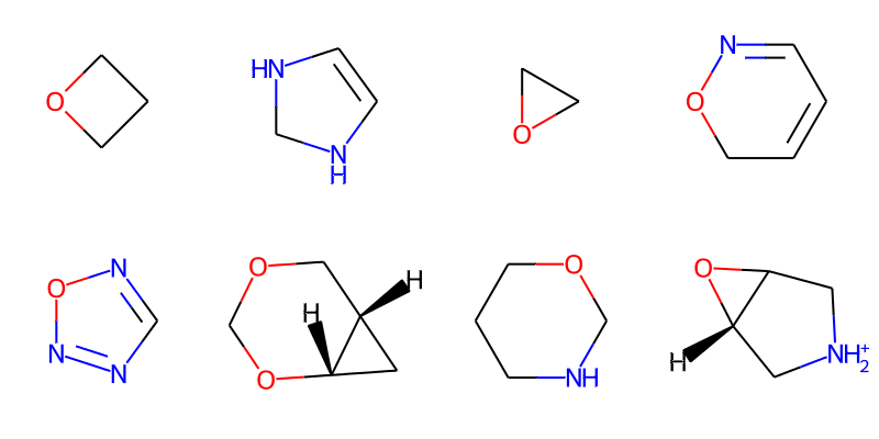
(a) QM9 Dataset

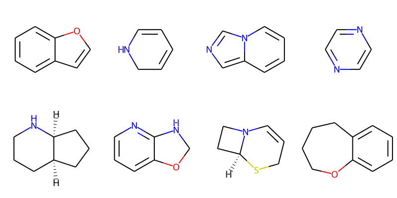
(b) ZINC250K Dataset

Figure 8: Examples of frequently occurring ring substructures

A.3 Equivariant Graph Neural Networks

Equivariant Graph Neural Networks (EGNN) (Satorras et al., 2021) are E(3)-equivariant with respect to an input set of points. The E(3) equivariance accounts for translation, rotation, and reflection symmetries, and can be extended to E($n$) group equivariance. The inherent dynamics governing the EGNN can be described, for each layer $l$, as follows. Here, $\mathbf{h}_{i}^{l}$ and $\mathbf{x}_{i}^{l}$ pertain, respectively, to the embedding for the node $i$ and that for its coordinates; and $a_{ij}$ abstracts the information about the edge between nodes $i$ and $j$.

$$\mathbf{m}_{ij} =\phi_{e}\left(\mathbf{h}_{i}^{l},\mathbf{h}_{j}^{l},\left\|\mathbf{x}_{i}^{l}-\mathbf{x}_{j}^{l}\right\|^{2},a_{ij}\right)$$

$$\mathbf{x}_{i}^{l+1} =\mathbf{x}_{i}^{l}+C\sum_{j\neq i}\left(\mathbf{x}_{i}^{l}-\mathbf{x}_{j}^{l}\right)\phi_{x}\left(\mathbf{m}_{ij}\right)$$

$$\mathbf{m}_{i} =\sum_{j\neq i}\mathbf{m}_{ij}$$

$$\mathbf{h}_{i}^{l+1} =\phi_{h}\left(\mathbf{h}_{i}^{l},\mathbf{m}_{i}\right)$$

Initially, messages $\mathbf{m}_{ij}$ are computed between the neighboring nodes via $\phi_{e}$. Subsequently, the coordinates of each node $i$ are updated via a weighted sum of relative position vectors $\{(\mathbf{x}_{i}-\mathbf{x}_{j}):j\neq i\}$ with the aid of $\phi_{x}$. Finally, the node embeddings are updated based on the aggregated messages $\mathbf{m}_{i}$ via $\phi_{h}$. The aggregated message can be computed based on only the neighbors of a node by simply replacing the sum over $j\neq i$ with a sum over $j\in\mathcal{N}_{i}$ in these equations.

A.4 Connection to Temporal Graph Networks

Temporal Graph Networks (Rossi et al., 2020; Souza et al., 2022) are state-of-the-art neural models for embedding dynamic graphs. A prominent class of these models consists of a combination of (recurrent) memory modules and graph-based operators, and rely on message passing for updating the embeddings based on node-wise or edge-wise events.

Specifically, adopting the notation from Rossi et al. (2020), an interaction $\mathbf{e}_{ij}(t)$ between any two nodes $i$ and $j$ at time $t$ triggers an edge-wise event leading to the following steps. First, a message $\mathbf{m}_{ij}^{\prime}(t)$ is computed based on the memory $\mathbf{s}_{i}\left(t^{-}\right)$ and $\mathbf{s}_{j}\left(t^{-}\right)$ of the two nodes just before time $t$ via a learnable function $\operatorname{msg}$ (such as multilayer perceptron). For each node $i$, the messages thus accrued over a small period due to interactions of with neighbors $j$ are combined (via $\operatorname{agg}$) into an aggregate message $\overline{\mathbf{m}}_{i}^{\prime}(t)$. This message, in turn, is used to update the memory of $i$ to $\mathbf{s}_{i}(t)$ via $\operatorname{mem}$ (implemented e.g., as a recurrent neural network). Finally, the node embedding of $i$ is revised based on its memory $\mathbf{s}_{i}(t)$, interaction $\mathbf{e}_{ij}(t)$ and memory $\mathbf{s}_{j}(t)$ of each neighbor $j\in\mathcal{N}_{i}$, as well as any additional node-wise events $\mathbf{v}_{i}(t)$ involving $i$ or any node in $\mathcal{N}_{i}$.

Table 7: ModFlow  as a temporal graph network (TGN). Adopting notation for TGNs from Rossi et al. (2020) $v_{i}$ is a node-wise event on $i$; $e_{ij}$ denotes an (asymmetric) interaction between $i$ and $j$; $\mathbf{s}_{i}$ is the memory of node $i$; and $t$ and $t^{-}$ denote time with $t^{-}$ being the time of last interaction before $t$, e.g., $\mathbf{s}_{i}(t^{-})$ is the memory of $i$ just before time $t$; and $\operatorname{msg}$ and $\operatorname{agg}$ are learnable functions (e.g., MLP) to compute, respectively, the individual and the aggregate messages. For ModFlow, we use $\mathbf{r}_{ij}$ to denote the spatial distance $\mathbf{x}_{i}-\mathbf{x}_{j}$, and $a_{ij}$ to denote the attributes of the edge between $i$ and $j$. The functions $\phi_{e}$, $\phi_{x}$, and $\phi_{h}$ are as defined in Satorras et al. (2021), and summarized in A.3.

Method	TGN layer	ModFlow
Edge	$\mathbf{m}_{ij}^{\prime}(t)=\operatorname{msg}\left(\mathbf{s}_{i}\left(t^{-}\right),\mathbf{s}_{j}\left(t^{-}\right),\Delta t,\mathbf{e}_{ij}(t)\right)$	$\mathbf{m}_{ij}(t)=\phi_{e}\left(\mathbf{z}_{i}(t),\mathbf{z}_{j}(t),\left\|\mathbf{r}_{ij}(t)\right\|^{2},a_{ij}\right)$
	$\overline{\mathbf{m}}_{i}^{\prime}(t)=\operatorname{agg}\left(\{\mathbf{m}_{ij}^{\prime}\left(t\right)|j\in\mathcal{N}_{i}\}\right)$	$\mathbf{m}_{i}(t)=\sum_{j\in\mathcal{N}(i)}\mathbf{m}_{ij}$
		$\hat{\mathbf{m}}_{ij}(t)=\mathbf{r}_{ij}(t)\cdot\phi_{x}\left(\mathbf{m}_{ij}(t)\right)$
		$\hat{\mathbf{m}}_{i}(t)=C\sum_{j\in\mathcal{N}(i)}\hat{\mathbf{m}}_{ij}(t)$
Memory state	$\mathbf{s}_{i}(t)=\operatorname{mem}\left(\overline{\mathbf{m}}_{i}^{\prime}(t),\mathbf{s}_{i}\left(t^{-}\right)\right)$	$\mathbf{x}_{i}(t+1)=\mathbf{x}_{i}(t)+\hat{\mathbf{m}}_{i}(t)$
Node	$\mathbf{z}_{i}^{\prime}(t)=\sum_{j\in\mathcal{N}_{i}}h\left(\mathbf{s}_{i}(t),\mathbf{s}_{j}(t),\mathbf{e}_{ij}(t),\mathbf{v}_{i}(t),\mathbf{v}_{j}(t)\right)$	$\mathbf{z}_{i}(t+1)=\phi_{h}\left(\mathbf{z}_{i}(t),\mathbf{m}_{i}(t)\right)$

It turns out (see Table 7) that ModFlow  can be viewed as an equivariant message passing temporal graph network. Interestingly, the coordinate embedding $\mathbf{x}_{i}$ plays the role of the memory $\mathbf{s}_{i}$.

A.5 Implementation Details

We implemented the proposed models in PyTorch (Paszke et al., 2019). We used a single layer for EGNN with embedding dimension 32 and aggregated information for each node from only its immediate neighbors. For geometric (spatial) information, we worked with the polar coordinates (2D) or the spherical polar coordinates (3D). We solved the ODE system with the Dormand–Prince adaptive step size scheme (i.e., the dopri5 solver). The number of function evaluations lay roughly between $70$ and $100$. The models were trained for 50-100 epochs with the Adam (Kingma and Ba, 2014) optimizer.

Time comparisons.

We found the training time of ModFlow  to be slightly worse than one-shot discrete flow models that characterize the whole system using a single flow (recall that, in contrast, ModFlow  associates an ODE with each node). However, ModFlow  is faster to train than the auto-regressive methods.

Note that computation is a crucial aspect of generative modeling for application domains with a huge search space, as is true for the molecules. We report the computational effort (excluding the time for preprocessing) for generating 10000 molecules averaged across 5 independent runs in Table 8. Notably, largely by virtue of being one-shot, ModFlow  is able to generate significantly faster than the auto-regressive models such as GraphAF and GraphDF. ModFlow  also owes this speedup, in part, to obviate the need for multiple decoding (unlike, e.g., JT-VAE) as well as any validity checks.

Table 8: Generation time (in seconds/molecule) on QM9 and ZINC250K.

Method	ZINC250K	QM9
GraphEBM	1.12 $\pm$ 0.34	0.53 $\pm$ 0.16
GVAE	0.86 $\pm$ 0.12	0.46 $\pm$ 0.07
GraphAF	0.93 $\pm$ 0.14	0.56 $\pm$ 0.12
GraphDF	3.12 $\pm$ 0.56	1.92 $\pm$ 0.42
MoFlow	0.71 $\pm$ 0.14	0.31 $\pm$ 0.04
ModFlow  (2D-EGNN)	0.46 $\pm$ 0.09	0.16 $\pm$ 0.04
ModFlow  (3D-EGNN)	0.55 $\pm$ 0.13	0.24 $\pm$ 0.06
ModFlow  (JT-2D-EGNN)	0.53 $\pm$ 0.07	0.21 $\pm$ 0.07
ModFlow  (JT-3D-EGNN)	0.62 $\pm$ 0.11	0.28 $\pm$ 0.09

A.6 Additional Evaluation Metrics

We invoked additional metrics, namely the MOSES metrics (Polykovskiy et al., 2020), to compare the different models in terms of their ability to generate molecules. These metrics, described below, access the overall quality of the generated molecules.

• FCD: Fréchet Chemnet Distance (FCD) (Preuer et al., 2018) is a general purpose metric that measures diversity of the generated molecules, as well as the extent of their chemical and biological property alignment with a reference set of real molecules. Specifically, the last layer activations of ChemNet are used for this purpose. Lower is better.

• Frag: Fragment similarity (Frag), measures the cosine distance between the fragment frequencies of the generated molecules and a set of reference molecules. Higher is better.

• SNN: Nearest Neighbor Similarity (SNN) quantifies how close the generated molecules are to the true molecule manifold. Specifically, it computes the average similarity of a generated molecule to the nearest molecule from the reference set. Higher is better.

• IntDiv: As the name suggests, Internal Diversity (IntDiv) accounts for diversity by computing the average pairwise similarity of the generated molecules. Higher is better.

For our purpose, we evaluated these metrics with QM9 and ZINC250K as the reference sets. As shown in Table 9 and Table 10, ModFlow  achieves better performance results across all metrics. Notably, ModFlow  registers lower FCD and higher IntDiv scores compared to other methods, suggesting that ModFlow  is able to generate diverse set of molecules similar to those present in the real datasets.

Table 9: Evaluation of performance on MOSES metrics on generative models on QM9 dataset. FCD is lower the better, Frag, SNN, and IntDiv higher the better.

Method	FCD ($\downarrow$)	Frag ($\uparrow$)	SNN ($\uparrow$)	IntDiv ($\uparrow$)
GVAE	0.513	0.821	0.582	0.822
GraphEBM	0.551	0.831	0.547	0.831
GraphAF	0.732	0.863	0.565	0.823
GraphDF	0.683	0.892	0.562	0.839
MoFlow	0.496	0.840	0.502	0.852
ModFlow  (2D-EGNN)	0.432	0.928	0.608	0.875
ModFlow  (3D-EGNN)	0.478	0.934	0.613	0.885
ModFlow  (JT-2D-EGNN)	0.421	0.921	0.595	0.867
ModFlow  (JT-3D-EGNN)	0.401	0.939	0.624	0.889

Table 10: Evaluation of performance on MOSES metrics on generative models on ZINC250K dataset. FCD is lower the better, Frag, SNN, and IntDiv higher the better.

Method	FCD ($\downarrow$)	Frag ($\uparrow$)	SNN ($\uparrow$)	IntDiv ($\uparrow$)
JTVAE	0.512	0.890	0.5477	0.855
GVAE	0.571	0.871	0.532	0.852
GraphEBM	0.613	0.843	0.487	0.821
GraphAF	0.524	0.803	0.465	0.855
GraphDF	0.658	0.869	0.515	0.829
MoFlow	0.597	0.851	0.452	0.832
ModFlow  (2D-EGNN)	0.495	0.891	0.570	0.863
ModFlow  (3D-EGNN)	0.512	0.905	0.584	0.869
ModFlow  (JT-2D-EGNN)	0.501	0.915	0.563	0.857
ModFlow  (JT-3D-EGNN)	0.523	0.929	0.594	0.879

We also evaluated the generated structures via distributions of their important properties. Specifically, we obtained kernel density estimates of these distributions to aid in visualization. We consider the following standard properties.

• Weight: sum of the individual atomic weights of a molecule. The weight provides insight into the bias of the generated molecules toward lighter or heavier molecules.

• LogP: ratio of concentration in octanol-phase to the aqueous phase, also known as the octanol-water partition coefficient. It is computed via the Crippen (Wildman and Crippen, 1999) estimation.

• Synthetic Accessibility (SA): an estimate for the synthesizability of a given molecule. It is calculated based on contributions of the molecule fragments Ertl and Schuffenhauer (2009).

• Quantitative Estimation of Drug-likeness (QED): describes the likeliness of a molecule as a viable candidate for a drug. It ranges between [0,1] and captures the abstract notion of aesthetics in medicinal chemistry (Bickerton et al., 2012).

Figure 9 and Figure 10 show that barring some dispersion in QED and logP (especially on Zinc250K), the property distributions of the molecules generated by ModFlow  generally match the corresponding distributions on the reference datasets quite closely. These results demonstrate the effectiveness of ModFlow  in generating molecules that have properties similar to the molecules in the reference set.

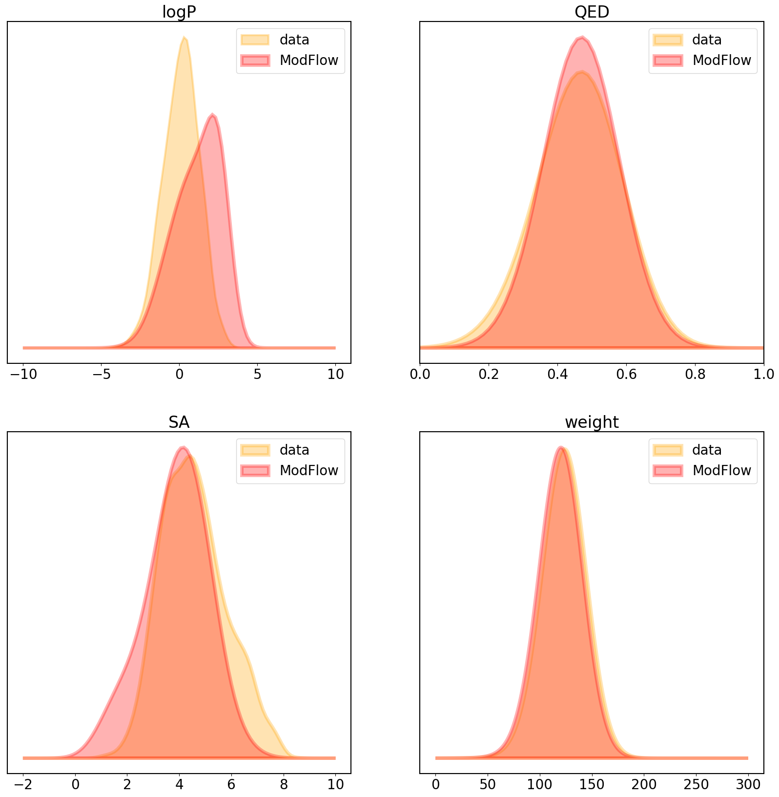
Figure 9: (QM9) Distributions of the chemical properties.

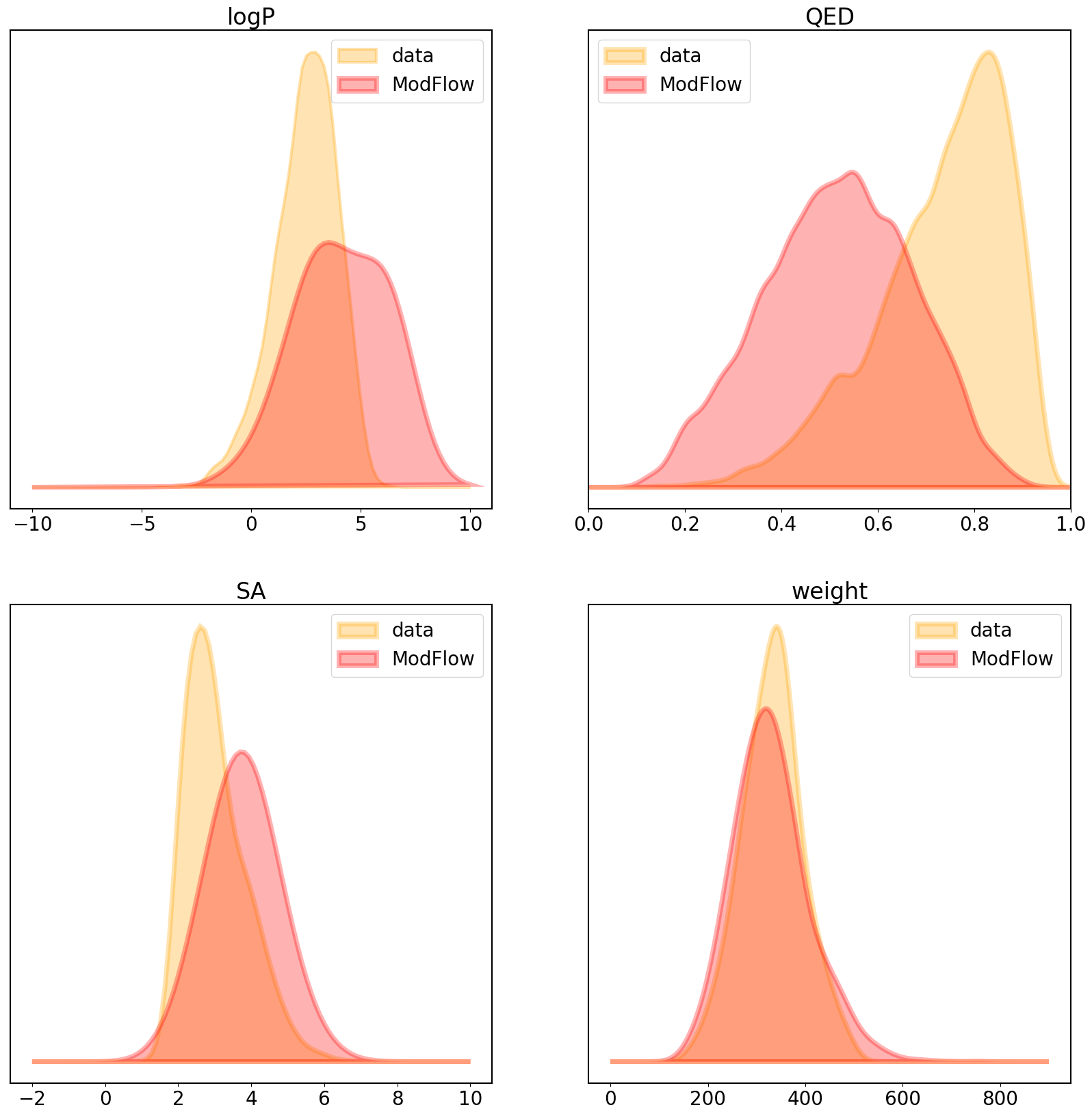
Figure 10: (ZINC250K) Distributions of the chemical properties.

A.7 Additional examples of molecules generated by ModFlow .

References

- Atwood and Towsley (2016) James Atwood and Don Towsley. Diffusion-convolutional neural networks. Advances in neural information processing systems, 29, 2016.
- Bickerton et al. (2012) G Richard Bickerton, Gaia V Paolini, Jérémy Besnard, Sorel Muresan, and Andrew L Hopkins. Quantifying the chemical beauty of drugs. Nature chemistry, 4(2):90–98, 2012.
- Bradley (2019) Andrew M. Bradley. PDE-constrained optimization and the adjoint method. Technical report, 2019.
- Chamberlain et al. (2021) Ben Chamberlain, James Rowbottom, Maria I Gorinova, Michael Bronstein, Stefan Webb, and Emanuele Rossi. Grand: Graph neural diffusion. In International Conference on Machine Learning, pages 1407–1418. PMLR, 2021.
- Chen et al. (2018) Ricky TQ Chen, Yulia Rubanova, Jesse Bettencourt, and David K Duvenaud. Neural ordinary differential equations. Advances in neural information processing systems, 31, 2018.
- Cramer et al. (2021) Eike Cramer, Alexander Mitsos, Raul Tempone, and Manuel Dahmen. Principal component density estimation for scenario generation using normalizing flows, 2021. URL https://arxiv.org/abs/2104.10410.
- Dai et al. (2018) Hanjun Dai, Yingtao Tian, Bo Dai, Steven Skiena, and Le Song. Syntax-directed variational autoencoder for structured data, 2018. URL https://arxiv.org/abs/1802.08786.
- Dinh et al. (2014) Laurent Dinh, David Krueger, and Yoshua Bengio. Nice: Non-linear independent components estimation. arXiv preprint arXiv:1410.8516, 2014.
- Dinh et al. (2016) Laurent Dinh, Jascha Sohl-Dickstein, and Samy Bengio. Density estimation using real nvp. arXiv preprint arXiv:1605.08803, 2016.
- Eliasof et al. (2021) Moshe Eliasof, Eldad Haber, and Eran Treister. Pde-gcn: Novel architectures for graph neural networks motivated by partial differential equations. Advances in Neural Information Processing Systems, 34, 2021.
- Ertl and Schuffenhauer (2009) Peter Ertl and Ansgar Schuffenhauer. Estimation of synthetic accessibility score of drug-like molecules based on molecular complexity and fragment contributions. Journal of cheminformatics, 1(1):1–11, 2009.
- Garg et al. (2020) Vikas Garg, Stefanie Jegelka, and Tommi Jaakkola. Generalization and representational limits of graph neural networks. In Proceedings of the 37th International Conference on Machine Learning, ICML 2020, 13-18 July 2020, Virtual Event, volume 119 of Proceedings of Machine Learning Research, pages 3419–3430. PMLR, 2020. URL http://proceedings.mlr.press/v119/garg20c.html.
- Goodfellow et al. (2014) Ian J. Goodfellow, Jean Pouget-Abadie, Mehdi Mirza, Bing Xu, David Warde-Farley, Sherjil Ozair, Aaron Courville, and Yoshua Bengio. Generative adversarial networks, 2014. URL https://arxiv.org/abs/1406.2661.
- Grathwohl et al. (2018) Will Grathwohl, Ricky TQ Chen, Jesse Bettencourt, Ilya Sutskever, and David Duvenaud. Ffjord: Free-form continuous dynamics for scalable reversible generative models. arXiv preprint arXiv:1810.01367, 2018.
- Honda et al. (2019) Shion Honda, Hirotaka Akita, Katsuhiko Ishiguro, Toshiki Nakanishi, and Kenta Oono. Graph residual flow for molecular graph generation. arXiv preprint arXiv:1909.13521, 2019.
- Huang et al. (2018) Chin-Wei Huang, David Krueger, Alexandre Lacoste, and Aaron Courville. Neural autoregressive flows, 2018. URL https://arxiv.org/abs/1804.00779.
- Iakovlev et al. (2020) Valerii Iakovlev, Markus Heinonen, and Harri Lähdesmäki. Learning continuous-time pdes from sparse data with graph neural networks. arXiv preprint arXiv:2006.08956, 2020.
- Ingraham et al. (2019) John Ingraham, Vikas Garg, Regina Barzilay, and Tommi Jaakkola. Generative models for graph-based protein design. In H. Wallach, H. Larochelle, A. Beygelzimer, F. d'Alché-Buc, E. Fox, and R. Garnett, editors, Advances in Neural Information Processing Systems, volume 32. Curran Associates, Inc., 2019. URL https://proceedings.neurips.cc/paper/2019/file/f3a4ff4839c56a5f460c88cce3666a2b-Paper.pdf.
- Irwin et al. (2012) John J Irwin, Teague Sterling, Michael M Mysinger, Erin S Bolstad, and Ryan G Coleman. Zinc: a free tool to discover chemistry for biology. Journal of chemical information and modeling, 52(7):1757–1768, 2012.
- Jin et al. (2018) Wengong Jin, Regina Barzilay, and Tommi Jaakkola. Junction tree variational autoencoder for molecular graph generation. arXiv preprint arXiv:1802.04364, 2018.
- Kajino (2019) Hiroshi Kajino. Molecular hypergraph grammar with its application to molecular optimization. In International Conference on Machine Learning, pages 3183–3191. PMLR, 2019.
- Kingma and Ba (2014) Diederik P Kingma and Jimmy Ba. Adam: A method for stochastic optimization. arXiv preprint arXiv:1412.6980, 2014.
- Kingma and Welling (2013) Diederik P Kingma and Max Welling. Auto-encoding variational bayes, 2013. URL https://arxiv.org/abs/1312.6114.
- Kobyzev et al. (2021) Ivan Kobyzev, Simon J.D. Prince, and Marcus A. Brubaker. Normalizing flows: An introduction and review of current methods. IEEE Transactions on Pattern Analysis and Machine Intelligence, 43(11):3964–3979, nov 2021. doi: 10.1109/tpami.2020.2992934. URL https://doi.org/10.1109%2Ftpami.2020.2992934.
- Kolmogorov et al. (1962) Andrei Nikolaevich Kolmogorov, Ye F Mishchenko, and Lev Semenovich Pontryagin. A probability problem of optimal control. Technical report, JOINT PUBLICATIONS RESEARCH SERVICE ARLINGTON VA, 1962.
- Kusner et al. (2017) Matt J. Kusner, Brooks Paige, and José Miguel Hernández-Lobato. Grammar variational autoencoder, 2017. URL https://arxiv.org/abs/1703.01925.
- Landrum et al. (2013) Greg Landrum et al. Rdkit: A software suite for cheminformatics, computational chemistry, and predictive modeling, 2013.
- Li et al. (2020) Zongyi Li, Nikola Kovachki, Kamyar Azizzadenesheli, Burigede Liu, Kaushik Bhattacharya, Andrew Stuart, and Anima Anandkumar. Neural operator: Graph kernel network for partial differential equations. arXiv preprint arXiv:2003.03485, 2020.
- Lim et al. (2018) Jaechang Lim, Seongok Ryu, Jin Woo Kim, and Woo Youn Kim. Molecular generative model based on conditional variational autoencoder for de novo molecular design. Journal of cheminformatics, 10(1):1–9, 2018.
- Lippe and Gavves (2021) Phillip Lippe and Efstratios Gavves. Categorical normalizing flows via continuous transformations. In International Conference on Learning Representations, 2021. URL https://openreview.net/forum?id=-GLNZeVDuik.
- Luo et al. (2021) Youzhi Luo, Keqiang Yan, and Shuiwang Ji. Graphdf: A discrete flow model for molecular graph generation, 2021. URL https://arxiv.org/abs/2102.01189.
- Madhawa et al. (2019) Kaushalya Madhawa, Katushiko Ishiguro, Kosuke Nakago, and Motoki Abe. Graphnvp: An invertible flow model for generating molecular graphs. arXiv preprint arXiv:1905.11600, 2019.
- Maziarka et al. (2020) Lukasz Maziarka, Agnieszka Pocha, Jan Kaczmarczyk, Krzysztof Rataj, Tomasz Danel, and Michał Warchoł. Mol-cyclegan: a generative model for molecular optimization. Journal of Cheminformatics, 12(1):1–18, 2020.
- Merz et al. (2020) Kenneth M. Merz, Gianni De Fabritiis, and Guo-Wei Wei. Generative models for molecular design. Journal of Chemical Information and Modeling, 60(12):5635–5636, 2020. doi: 10.1021/acs.jcim.0c01388. URL https://doi.org/10.1021/acs.jcim.0c01388. PMID: 33378853.
- Neil et al. (2018) Daniel Neil, Marwin Segler, Laura Guasch, Mohamed Ahmed, Dean Plumbley, Matthew Sellwood, and Nathan Brown. Exploring deep recurrent models with reinforcement learning for molecule design. 2018.
- Papamakarios et al. (2021) George Papamakarios, Eric Nalisnick, Danilo Jimenez Rezende, Shakir Mohamed, and Balaji Lakshminarayanan. Normalizing flows for probabilistic modeling and inference. Journal of Machine Learning Research, 22(57):1–64, 2021.
- Paszke et al. (2019) Adam Paszke, Sam Gross, Francisco Massa, Adam Lerer, James Bradbury, Gregory Chanan, Trevor Killeen, Zeming Lin, Natalia Gimelshein, Luca Antiga, et al. Pytorch: An imperative style, high-performance deep learning library. Advances in neural information processing systems, 32, 2019.
- Poli et al. (2019) Michael Poli, Stefano Massaroli, Junyoung Park, Atsushi Yamashita, Hajime Asama, and Jinkyoo Park. Graph neural ordinary differential equations. arXiv preprint arXiv:1911.07532, 2019.
- Polishchuk et al. (2013) Pavel G Polishchuk, Timur I Madzhidov, and Alexandre Varnek. Estimation of the size of drug-like chemical space based on gdb-17 data. Journal of computer-aided molecular design, 27(8):675–679, 2013.
- Polykovskiy et al. (2020) Daniil Polykovskiy, Alexander Zhebrak, Benjamin Sanchez-Lengeling, Sergey Golovanov, Oktai Tatanov, Stanislav Belyaev, Rauf Kurbanov, Aleksey Artamonov, Vladimir Aladinskiy, Mark Veselov, Artur Kadurin, Simon Johansson, Hongming Chen, Sergey Nikolenko, Alan Aspuru-Guzik, and Alex Zhavoronkov. Molecular Sets (MOSES): A Benchmarking Platform for Molecular Generation Models. Frontiers in Pharmacology, 2020.
- Popova et al. (2019) Mariya Popova, Mykhailo Shvets, Junier Oliva, and Olexandr Isayev. Molecularrnn: Generating realistic molecular graphs with optimized properties, 2019. URL https://arxiv.org/abs/1905.13372.
- Preuer et al. (2018) Kristina Preuer, Philipp Renz, Thomas Unterthiner, Sepp Hochreiter, and Gunter Klambauer. Fréchet chemnet distance: a metric for generative models for molecules in drug discovery. Journal of chemical information and modeling, 58(9):1736–1741, 2018.
- Ramakrishnan et al. (2014) Raghunathan Ramakrishnan, Pavlo O Dral, Matthias Rupp, and O Anatole von Lilienfeld. Quantum chemistry structures and properties of 134 kilo molecules. Scientific Data, 1, 2014.
- Ramesh et al. (2022) Aditya Ramesh, Prafulla Dhariwal, Alex Nichol, Casey Chu, and Mark Chen. Hierarchical text-conditional image generation with clip latents, 2022. URL https://arxiv.org/abs/2204.06125.
- Rossi et al. (2020) Emanuele Rossi, Ben Chamberlain, Fabrizio Frasca, Davide Eynard, Federico Monti, and Michael Bronstein. Temporal graph networks for deep learning on dynamic graphs, 2020. URL https://arxiv.org/abs/2006.10637.
- Samanta et al. (2018) Bidisha Samanta, Abir De, Niloy Ganguly, and Manuel Gomez-Rodriguez. Designing random graph models using variational autoencoders with applications to chemical design. arXiv preprint arXiv:1802.05283, 2018.
- Satorras et al. (2021) Victor Garcia Satorras, Emiel Hoogeboom, and Max Welling. E(n) equivariant graph neural networks, 2021. URL https://arxiv.org/abs/2102.09844.
- Scarselli et al. (2009) Franco Scarselli, Marco Gori, Ah Chung Tsoi, Markus Hagenbuchner, and Gabriele Monfardini. The graph neural network model. IEEE Transactions on Neural Networks, 20(1):61–80, 2009. doi: 10.1109/TNN.2008.2005605.
- Segler et al. (2018) Marwin HS Segler, Thierry Kogej, Christian Tyrchan, and Mark P Waller. Generating focused molecule libraries for drug discovery with recurrent neural networks. ACS central science, 4(1):120–131, 2018.
- Shi et al. (2020) Chence Shi, Minkai Xu, Zhaocheng Zhu, Weinan Zhang, Ming Zhang, and Jian Tang. Graphaf: a flow-based autoregressive model for molecular graph generation. arXiv preprint arXiv:2001.09382, 2020.
- Souza et al. (2022) Amauri Souza, Diego Mesquita, Samuel Kaski, and Vikas Garg. Provably expressive temporal graph networks. In Advances in Neural Information Processing Systems (NeurIPS), 2022.
- Stokes et al. (2020) Jonathan M. Stokes, Kevin Yang, Kyle Swanson, Wengong Jin, Andres Cubillos-Ruiz, Nina M. Donghia, Craig R. MacNair, Shawn French, Lindsey A. Carfrae, Zohar Bloom-Ackermann, Victoria M. Tran, Anush Chiappino-Pepe, Ahmed H. Badran, Ian W. Andrews, Emma J. Chory, George M. Church, Eric D. Brown, Tommi S. Jaakkola, Regina Barzilay, and James J. Collins. A deep learning approach to antibiotic discovery. Cell, 180(4):688–702.e13, 2020. ISSN 0092-8674. doi: https://doi.org/10.1016/j.cell.2020.01.021. URL https://www.sciencedirect.com/science/article/pii/S0092867420301021.
- Weininger (1988) David Weininger. Smiles, a chemical language and information system. 1. introduction to methodology and encoding rules. Journal of chemical information and computer sciences, 28(1):31–36, 1988.
- Wildman and Crippen (1999) Scott A Wildman and Gordon M Crippen. Prediction of physicochemical parameters by atomic contributions. Journal of chemical information and computer sciences, 39(5):868–873, 1999.
- Xhonneux et al. (2020) Louis-Pascal Xhonneux, Meng Qu, and Jian Tang. Continuous graph neural networks. In International Conference on Machine Learning, pages 10432–10441. PMLR, 2020.
- You et al. (2018) Jiaxuan You, Rex Ying, Xiang Ren, William Hamilton, and Jure Leskovec. Graphrnn: Generating realistic graphs with deep auto-regressive models. In International conference on machine learning, pages 5708–5717. PMLR, 2018.
- Zang and Wang (2020) Chengxi Zang and Fei Wang. Moflow: an invertible flow model for generating molecular graphs. In Proceedings of the 26th ACM SIGKDD International Conference on Knowledge Discovery & Data Mining, pages 617–626, 2020.
- Zhen et al. (2020) Xingjian Zhen, Rudrasis Chakraborty, Liu Yang, and Vikas Singh. Flow-based generative models for learning manifold to manifold mappings, 2020. URL https://arxiv.org/abs/2012.10013.