Probabilities Are Not Enough: Formal Controller Synthesis for
Stochastic Dynamical Models with Epistemic Uncertainty

Abstract

Capturing uncertainty in models of complex dynamical systems is crucial to designing safe controllers. Stochastic noise causes aleatoric uncertainty, whereas imprecise knowledge of model parameters leads to epistemic uncertainty. Several approaches use formal abstractions to synthesize policies that satisfy temporal specifications related to safety and reachability. However, the underlying models exclusively capture aleatoric but not epistemic uncertainty, and thus require that model parameters are known precisely. Our contribution to overcoming this restriction is a novel abstraction-based controller synthesis method for continuous-state models with stochastic noise and uncertain parameters. By sampling techniques and robust analysis, we capture both aleatoric and epistemic uncertainty, with a user-specified confidence level, in the transition probability intervals of a so-called interval Markov decision process (iMDP). We synthesize an optimal policy on this iMDP, which translates (with the specified confidence level) to a feedback controller for the continuous model with the same performance guarantees. Our experimental benchmarks confirm that accounting for epistemic uncertainty leads to controllers that are more robust against variations in parameter values.

1 Introduction

Stochastic models.

Stochastic dynamical models capture complex systems where the likelihood of transitions is specified by probabilities (Kumar and Varaiya 2015). Controllers for stochastic models must act safely and reliably with respect to a desired specification. Traditional control design methods use, e.g., Lyapunov functions and optimization to guarantee stability and (asymptotic) convergence. However, alternative methods are needed to give formal guarantees about richer temporal specifications relevant to, for example, safety-critical applications (Fan et al. 2022).

Finite abstractions.

A powerful approach to synthesizing certifiably safe controllers leverages probabilistic verification to provide formal guarantees over specifications of safety (always avoid certain states) and reachability (reach a certain set of states). A common example is the reach-avoid specification, where the task is to maximize the probability of reaching desired goal states while avoiding unsafe states (Fisac et al. 2015). Finite abstractions can make continuous models amenable to techniques and tools from formal verification: by discretizing their state and action spaces, abstractions result in, e.g., finite Markov decision processes (MDPs) that soundly capture the continuous dynamics (Abate et al. 2008). Verification guarantees on the finite abstraction can thus carry over to the continuous model. In this paper, we adopt such an abstraction-based approach to controller synthesis.

Probabilities are not enough.

The notion of uncertainty is often distinguished in aleatoric (statistical) and epistemic (systematic) uncertainty (Fox and Ülkümen 2011; Sullivan 2015). Epistemic uncertainty is, in particular, modeled by parameters that are not precisely known (Smith 2013). A general premise is that purely probabilistic approaches fail to capture epistemic uncertainty (Hüllermeier and Waegeman 2021). In this work, we aim to reason under both aleatoric and epistemic uncertainty in order to synthesize provably correct controllers for safety-critical applications. Existing abstraction methods fail to achieve this novel, general goal.

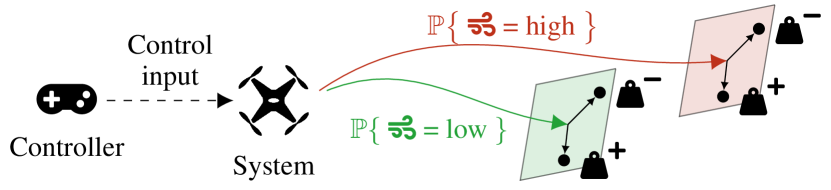
Figure 1: Aleatoric (stochastic) uncertainty in the wind (wind) causes probability distributions over the outcomes of controls, while epistemic uncertainty in the mass (weight-hanging) of the drone causes state transitions to be nondeterministic.

Models with epistemic uncertainty.

We consider reach-avoid problems for stochastic dynamical models with continuous state and action spaces under epistemic uncertainty described by parameters that lie within a convex uncertainty set. In the simplest case, this uncertainty set is an interval, such as a drone whose mass is only known to lie between $0.75$–$1.25\text{\,}\mathrm{kg}$. As shown in Fig. 1, the dynamics of the drone depend on uncertain factors, such as the wind and the drone’s mass. For the wind, we may derive a probabilistic model from, e.g., weather data to reason over the likelihood of state dynamics. For the mass, however, we do not have information about the likelihood of each value, so employing a probabilistic model is unrealistic. Thus, we treat epistemic uncertainty in such imprecisely known parameters (in this case, the mass) using a nondeterministic framework instead.

Problem statement.

Our goal is to synthesize a controller that (1) is robust against nondeterminism due to parameter uncertainty and (2) reasons over probabilities derived from stochastic noise. In other words, the controller must satisfy a given specification under any possible outcome of the nondeterminism (robustness) and with at least a certain probability regarding the stochastic noise (reasoning over probabilities). We wish to synthesize a controller with a probably approximately correct (PAC)-style guarantee to satisfy a reach-avoid specification with at least a desired threshold probability. Thus, we solve the following problem:

Problem. Given a reach-avoid specification for a stochastic model with uncertain parameters, compute a controller and a lower bound on the probability that, under any admissible value of the parameters, the specification is probabilistically satisfied with this lower bound and with at least a user-specified confidence probability.

We solve this problem via a discrete-state abstraction of the continuous model. We generate this abstraction by partitioning the continuous state space and defining actions that induce potential transitions between elements of this partition.

Algorithmically, the closest approach to ours is Badings et al. (2022), which uses abstractions to synthesize controllers for stochastic models with aleatoric uncertainty of unknown distribution, but with known parameters. Our setting is more general, as epistemic uncertainty requires fundamental differences to the technical approach, as explained below.

Robustness to capture nondeterminism.

The main contribution that allows us to capture nondeterminism, is that we reason over sets of potential transitions (as shown by the boxes in Fig. 1), rather than precise transitions, e.g., as in Badings et al. (2022). Intuitively, for a given action, the aleatoric uncertainty creates a probability distribution over sets of possible outcomes. To ensure robustness against epistemic uncertainty, we consider all possible outcomes within these sets. We show that, for our class of models, computing these sets of all possible outcomes is computationally tractable. Building upon this reasoning, we provide the following guarantees to solve the above-mentioned problem.

1) PAC guarantees on abstractions.

We show that both probabilities and nondeterminism can be captured in the transition probability intervals of so-called interval Markov decision processes (iMDPs, Givan, Leach, and Dean 2000). We use sampling methods from scenario optimization (Campi, Carè, and Garatti 2021) and concentration inequalities (Boucheron, Lugosi, and Massart 2013) to compute PAC bounds on these intervals. With a predefined confidence probability, the iMDP correctly captures both aleatoric and epistemic uncertainty.

2) Correct-by-construction control.

For the iMDP, we compute a robust optimal policy that maximizes the worst-case probability of satisfying the reach-avoid specification. The iMDP policy is automatically translated to a controller for the original, continuous model on the fly. We show that, by construction, the PAC guarantees on the iMDP carry over to the satisfaction of the specification by the continuous model.

Contributions.

We develop the first abstraction-based, formal controller synthesis method that simultaneously captures epistemic and aleatoric uncertainty for models with continuous state and action spaces. We also provide results on the PAC-correctness of obtained iMDP abstractions and guarantees on the synthesized controllers for a reach-avoid specification. Our numerical experiments in Sect. 6 confirm that accounting for epistemic uncertainty yields controllers that are more robust against deviations in the parameter values.

Related Work

Uncertainty models.

Distinguishing aleatoric from epistemic uncertainty is a key challenge towards trustworthy AI (Thiebes, Lins, and Sunyaev 2021), and has been considered in reinforcement learning (Charpentier et al. 2022), Bayesian neural networks (Depeweg et al. 2018; Loquercio, Segù, and Scaramuzza 2020), and systems modeling (Smith 2013). Dynamical models with epistemic parameter uncertainty (but without aleatoric uncertainty) are considered by Yedavalli (2014), and Geromel and Colaneri (2006). Control of models similar to ours is studied by (Modares 2022), albeit only for stability specifications.

Model-based approaches.

Abstractions of stochastic models are a well-studied research area (Abate et al. 2008; Alur et al. 2000), with applications to stochastic hybrid (Cauchi et al. 2019; Lavaei et al. 2022), switched (Lahijanian, Andersson, and Belta 2015), and partially observable systems (Badings et al. 2021; Haesaert et al. 2018). Various tools exist, e.g., StocHy (Cauchi and Abate 2019), ProbReach (Shmarov and Zuliani 2015), and SReachTools (Vinod, Gleason, and Oishi 2019). However, in contrast to the approach of this paper, none of these papers deals with epistemic uncertainty.

Fan et al. (2022) use optimization for reach-avoid control of linear but non-stochastic models with bounded disturbances. Barrier functions are used for cost minimization in stochastic optimal control (Pereira et al. 2020). So-called funnel libraries are used by Majumdar and Tedrake (2017) for robust feedback motion planning under epistemic uncertainty. Finally, Zikelic et al. (2022) learn policies together with formal reach-avoid certificates using neural networks for nonlinear systems with only aleatoric uncertainty.

Data-driven approaches.

Models with (partly) unknown dynamics express epistemic uncertainty about the underlying system. Verification of such models based on data has been done using Bayesian inference (Haesaert, den Hof, and Abate 2017), optimization (Kenanian et al. 2019; Vinod, Israel, and Topcu 2022), and Gaussian process regression (Jackson et al. 2020). Moreover, Knuth et al. (2021), and Chou, Ozay, and Berenson (2021) use neural network models for feedback motion planning for nonlinear deterministic systems with probabilistic safety and reachability guarantees. Data-driven abstractions have been developed for monotone (Makdesi, Girard, and Fribourg 2021) and event-triggered systems (Peruffo and Mazo 2023). By contrast to our setting, these approaches consider models with non-stochastic dynamics. A few recent exceptions also consider aleatoric uncertainty (Salamati and Zamani 2022; Lavaei et al. 2023), but these approaches require more strict assumptions (e.g., discrete input sets) than our model-based approach.

Safe learning.

While outside the scope of this paper, our approach fits naturally in a model-based safe learning context (Brunke et al. 2022; García and Fernández 2015). In such a setting, our approach may synthesize controllers that guarantee safe interactions with the system, while techniques from, for example, reinforcement learning (RL, Berkenkamp et al. 2017; Zanon and Gros 2021) or stochastic system identification (Tsiamis and Pappas 2019) can reduce the epistemic uncertainty based on state observations. A risk-sensitive RL scheme providing approximate safety guarantees is developed by Geibel and Wysotzki (2005); we instead give formal guarantees at the cost of an expensive abstraction.

2 Problem Statement

The cardinality of a discrete set $\mathcal{X}$ is $|\mathcal{X}|$. A probability space is a triple $(\Omega,\mathcal{F},\amsmathbb{P})$ of an arbitrary set $\Omega$, sigma algebra $\mathcal{F}$ on $\Omega$, and probability measure $\amsmathbb{P}\colon\mathcal{F}\to[0,1]$. The convex hull of a polytopic set $\mathcal{X}$ with vertices $v_{1},\ldots,v_{n}$ is $\mathrm{conv}(v_{1},\ldots,v_{n})$. The word controller relates to continuous models; a policy to discrete models.

Stochastic Models with Parameter Uncertainty

To capture parameter uncertainty in a linear time-invariant stochastic system, we consider a model (we extend this model with parameters describing uncertain additive disturbances in Sect. 5) whose continuous state $x_{k}$ at time $k\in\amsmathbb{N}$ evolves as

$$x_{k+1}=A(\alpha)x_{k}+B(\alpha)u_{k}+\eta_{k},$$ (1)

where $u_{k}\in\mathcal{U}$ is the control input, which is constrained by the control space $\mathcal{U}=\mathrm{conv}(u^{1},\ldots,u^{q})\subset\amsmathbb{R}^{m}$, being is a convex polytope with $q$ vertices, and where the process noise $\eta_{k}$ is a stochastic process defined on a probability space $(\Omega,\mathcal{F},\amsmathbb{P})$. Both the dynamics matrix $A(\alpha)\in\amsmathbb{R}^{n\times n}$ and the control matrix $B(\alpha)\in\amsmathbb{R}^{n\times m}$ are a convex combination of a finite set of $r\in\amsmathbb{N}$ known matrices:

$$A(\alpha) =\sum\nolimits_{i=1}^{r}\alpha_{i}A_{i},\enskip B(\alpha)=\sum\nolimits_{i=1}^{r}\alpha_{i}B_{i},\enskip$$ (2)

where the unknown model parameter $\alpha\in\Gamma$ can be any point in the unit simplex $\Gamma\subset\amsmathbb{R}^{r}$:

$$\Gamma =\Big{\{}\alpha\in\amsmathbb{R}^{r}\colon\alpha_{i}\geq 0,~{}\forall i\in\{1,\ldots,r\},\enskip\sum\nolimits_{i=1}^{r}\alpha_{i}=1\Big{\}}.$$

The model in Eq. 1 captures epistemic uncertainty in $A(\alpha)$ and $B(\alpha)$ through model parameter $\alpha$, as well as aleatoric uncertainty in the discrete-time stochastic process $(\eta_{k})_{k\in\amsmathbb{N}}$.

Assumption 1.

The noise $\eta_{k}$ is independent and identically distributed (i.i.d., which is a common assumption) and has density with respect to the Lebesgue measure. However, contrary to most definitions, we allow $\amsmathbb{P}$ to be unknown.

Importantly, being distribution-free, our proposed techniques hold for any distribution of $\eta$ that satisfies Assumption 1.

The matrices $A_{i}$ and $B_{i}$ can represent the bounds of intervals over parameters, as illustrated by the following example.

Example 1.

Consider again the drone of Fig. 1. The drone’s longitudinal position $p_{k}$ and velocity $v_{k}$ are modeled as

$$x_{k+1}=\begin{bmatrix}p_{k+1}\\ v_{k+1}\end{bmatrix}=\begin{bmatrix}1&\tau\\ 0&1-\frac{0.1\tau}{m}\end{bmatrix}x_{k}+\begin{bmatrix}\frac{\tau^{2}}{2m}\\ \frac{\tau}{m}\end{bmatrix}u_{k}+\eta_{k},$$

with $\tau$ the discretization time, and $\mathcal{U}=[-5,5]$. Assume that the mass $m$ is only known to lie within $[0.75,1.25]$. Then, we obtain a model as Eq. 1, with $r=2$ vertices where $A_{1},B_{1}$ are obtained for $m\coloneqq 0.75$, and $A_{2},B_{2}$ for $m\coloneqq 1.25$. ∎

Reach-Avoid Planning Problem

The goal is to steer the state $x_{k}$ of Eq. 1 to a desirable state within $K$ time steps while always remaining in a safe region. Formally, let the safe set $\mathcal{Z}$ be a compact set of $\amsmathbb{R}^{n}$, and let $\mathcal{G}\subseteq\mathcal{Z}$ be the goal set (see Fig. 2). The control inputs $u_{k}$ in Eq. 1 are selected by a time-varying feedback controller:

Definition 1.

A time-varying feedback controller $c\colon\amsmathbb{R}^{n}\times\amsmathbb{N}\to\mathcal{U}$ for Eq. 1 is a function that maps a state $x_{k}\in\amsmathbb{R}^{n}$ and a time step $k\in\amsmathbb{N}$ to a control input $u_{k}\in\mathcal{U}$.

The space of admissible feedback controllers is denoted by $\mathcal{C}$. The reach-avoid probability $V(x_{0},\alpha,c)$ is the probability that Eq. 1, under parameter $\alpha\in\Gamma$ and a controller $c$, satisfies a reach-avoid planning problem with respect to the sets $\mathcal{Z}$ and $\mathcal{G}$, starting from initial state $x_{0}\in\amsmathbb{R}^{n}$. Formally:

Definition 2.

The reach-avoid probability $V\colon\amsmathbb{R}^{n}\times\Gamma\times\mathcal{C}\to[0,1]$ for a given controller $c\in\mathcal{C}$ on horizon $K$ is

$$\begin{split}V(x_{0},&\ \alpha,c)=\amsmathbb{P}\big{\{}\eta_{k}\in\Omega\,\colon\,x_{k}\text{ evolves as per \lx@cref{creftype~refnum}{eq:uncertain_LTI_model}},\\ &\exists k^{\prime}\in\{0,\ldots,K\}\,\,\text{such that}\,\,x_{k^{\prime}}\in\mathcal{G},\text{ and}\\ &x_{k}\in\mathcal{Z},\,u_{k}=c(x_{k},k)\,\,\forall k\in\{0,\ldots,k^{\prime}\}\big{\}}.\end{split}$$

We aim to find a controller for which the reach-avoid probability is above a certain threshold $\lambda\in[0,1]$. However, since parameter $\alpha$ of Eq. 1 is unknown, it is impossible to compute the reach-avoid probability explicitly. We instead take a robust approach, thus stating the formal problem as follows:

Formal problem.

Given an initial state $x_{0}$, find a controller $c\in\mathcal{C}$ together with a (high) probability threshold $\lambda\in[0,1]$, such that $V(x_{0},\alpha,c)\geq\lambda$ holds for all $\alpha\in\Gamma$.

Thus, we want to find a controller $c\in\mathcal{C}$ that is robust against any possible instance of parameter $\alpha\in\Gamma$ in Eq. 1. Due to the aleatoric uncertainty in Eq. 1 of unknown distribution, we solve the problem up to a user-specified confidence probability $\beta\in(0,1)$, as we shall see in Sect. 5.

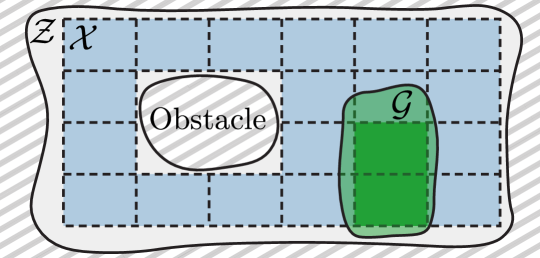
Figure 2: Partition of safe set $\mathcal{X}\subseteq\mathcal{Z}$ (which excludes obstacles) into regions that define iMDP states. A state $s_{i}$ is a goal state, $s_{i}\in S_{\mathcal{G}}$, if its region is contained in the goal region $\mathcal{G}$.

Interval Markov Decision Processes

We solve the problem by generating a finite-state abstraction of the model as an interval Markov decision process (iMDP):

Definition 3.

An iMDP is a tuple $\mathcal{M}{I}=(S,Act,s_{I},\mathcal{P})$ where $S$ is a finite set of states, $Act$ is a finite set of actions, $s_{I}\in S$ is the initial state, and $\mathcal{P}\colon S\times Act\times S\to\amsmathbb{I}\cup\{[0,0]\}$ is an uncertain partial probabilistic transition function over intervals $\amsmathbb{I}=\{[a,b]\ |\ a,b\in(0,1]\text{ and }a\leq b\}$.

Note that an interval may not have a lower bound of $0$, except for the $[0,0]$ interval. If $\mathcal{P}(s,a,s^{\prime})=[0,0]\,\forall s^{\prime}\in S$, action $a\in Act$ is not enabled in state $s\in S$. We can instantiate an iMDP into an MDP with a partial transition function $P\colon S\times Act\rightharpoonup\mathit{Dist(S)}$ by fixing a probability $P(s,a)(s^{\prime})\in\mathcal{P}(s,a,s^{\prime})$ for each $s,s^{\prime}\in S$ and for each $a\in Act$ enabled in $s$, such that $P(s,a)$ is a probability distribution over $S$. For brevity, we write this instantiation as $P\in\mathcal{P}$ and denote the resulting MDP by $\mathcal{M}{I}[P]$.

A deterministic policy (Baier and Katoen 2008) for an iMDP $\mathcal{M}{I}$ is a function $\pi\colon S^{\ast}\to Act$, where $S^{\ast}$ is a sequence of states (memoryless policies do not suffice for time-bounded specifications), with $\pi\in\Pi_{\mathcal{M}{I}}$ the admissible policy space. For a policy $\pi$ and an instantiated MDP $\mathcal{M}{I}[P]$ for $P\in\mathcal{P}$, we denote by $Pr^{\pi}(\mathcal{M}{I}[P]\models\varphi_{s_{I}}^{K})$ the probability of satisfying a reach-avoid specification $\varphi_{s_{I}}^{K}$ (i.e., reaching a goal in $S_{\mathcal{G}}\subseteq S$ within $K\in\amsmathbb{N}$ steps, while not leaving a safe set $S_{\mathcal{Z}}\subseteq S$). A robust optimal policy $\pi^{\star}\in\Pi_{\mathcal{M}{I}}$ maximizes this probability under the minimizing instantiation $P\in\mathcal{P}$:

$$\begin{split}\pi^{\star}&=\operatorname*{arg\,max}_{\pi\in\Pi}\min_{P\in\mathcal{P}}Pr^{\pi}(\mathcal{M}{I}[P]\models\varphi_{s_{I}}^{K}).\end{split}$$ (3)

We compute an optimal policy in Eq. 3 using a robust variant of value iteration proposed by Wolff, Topcu, and Murray (2012). Note that deterministic policies suffice to obtain optimal values for Eq. 3, see Puggelli et al. (2013).

3 Finite-State Abstraction

To solve the formal problem, we construct a finite-state abstraction of Eq. 1 as an iMDP. We define the actions of this iMDP via backward reachability computations on a so-called nominal model that neglects any source of uncertainty. We then compensate for the error caused by this modeling simplification in the iMDP’s transition probability intervals.

Nominal Model of the Dynamics

To build our abstraction, we rely on a nominal model that neglects both the aleatoric and epistemic uncertainty in Eq. 1, and is thus deterministic. Concretely, we fix any value $\hat{\alpha}\in\Gamma$ and define the nominal model dynamics as

$$\hat{x}_{k+1}=A(\hat{\alpha})x_{k}+B(\hat{\alpha})u_{k}.$$ (4)

Due to the linearity of the dynamics, we can now express the successor state $x_{k+1}$ with full uncertainty, from Eq. 1, as

$$x_{k+1}=\hat{x}_{k+1}+\delta(\alpha,x_{k},u_{k})+\eta_{k},$$ (5)

with $\delta(\alpha,x_{k},u_{k})$ being a new term, called the epistemic error, encompassing the error caused by parameter uncertainty:

$$\delta(\alpha,x_{k},u_{k})=[A(\alpha)-A(\hat{\alpha})]x_{k}+[B(\alpha)-B(\hat{\alpha})]u_{k}.$$ (6)

In other words, the successor state $x_{k+1}$ is the nominal one, plus the epistemic error, and plus the stochastic noise. Note that for $\alpha=\hat{\alpha}$ (i.e., the true model parameters equal their nominal values), we obtain $\delta(\alpha,x_{k},u_{k})=0$. We also impose the next assumption on the nominal model, which guarantees that we can compute the inverse image of Eq. 4 for a given $\hat{x}_{k+1}$, and is used in the proof of Lemma 3 in Appendix A.

Assumption 2.

The matrix $A(\hat{\alpha})$ in Eq. 4 is non-singular.

Assumption Assumption 2 is mild as it only requires the existence of a non-singular matrix in $\mathrm{conv}\{A_{1},\ldots,A_{r}\}$.

States

We create a partition of a subset $\mathcal{X}$ of the safe set $\mathcal{Z}$ on the continuous state space, see Fig. 2. This partition fully covers the goal set $\mathcal{G}$ but excludes unsafe states, i.e., any $x\notin\mathcal{Z}$.

Definition 4.

A finite collection of subsets $(\mathcal{P}_{i})_{i=1}^{L}$ is called a partition of $\mathcal{X}\subseteq\mathcal{Z}\subset\amsmathbb{R}^{n}$ if the following conditions hold:

1. $\mathcal{X}=\bigcup_{i=1}^{L}\mathcal{P}_{i}$,

2. $\mathcal{P}_{i}\bigcap\mathcal{P}_{j}=\emptyset,\,\,\forall i,j\in\{1,\ldots,L\},\,\,i\neq j$.

We append to the partition a so-called absorbing region $\mathcal{P}_{0}=\mathrm{cl}(\amsmathbb{R}^{n}\setminus\mathcal{X})$, which is defined as the closure of $\amsmathbb{R}^{n}\setminus\mathcal{X}$ and represents any state $x\notin\mathcal{X}$ that is disregarded in subsequent reachability computations. We consider partitions into convex polytopic regions, which will allow us to compute PAC probability intervals in Lemma 1 using results from Romao, Papachristodoulou, and Margellos (2022) on scenario optimization programs with discarded constraints:

Assumption 3.

Each region $\mathcal{P}_{i}$ is a convex polytope given by

$$\mathcal{P}_{i} =\{x\in\amsmathbb{R}^{n}\colon H_{i}x\leq h_{i}\},$$ (7)

with $H_{i}\in\amsmathbb{R}^{p_{i}\times n}$ and $h_{i}\in\amsmathbb{R}^{p_{i}}$ for some $p_{i}\in\amsmathbb{N}$, and the inequality in Eq. 7 is to be interpreted element-wise.

We define an iMDP state for each element of $(\mathcal{P}_{i})_{i=0}^{L}$, yielding a set of $L+1$ discrete states $S=\{s_{i}\mid i=0,\ldots,L\}$. Define $T\colon\amsmathbb{R}^{n}\to\{0,1,\dots,L\}$ as the map from any $x\in\mathcal{X}$ to its corresponding region index $i$. We say that a continuous state $x$ belongs to iMDP state $s_{i}$ if $T(x)=i$. State $s_{0}$ is a deadlock, such that the only transition leads back to $s_{0}$.

Actions

Recall that we define the iMDP actions via backward reachability computations under the nominal model in Eq. 4. Let $\mathcal{T}=\{\mathcal{T}_{1},\ldots,\mathcal{T}_{M}\}$ be a finite collection of target sets, each of which is a convex polytope, $\mathcal{T}_{\ell}=\mathrm{conv}\{t^{1},\ldots,t^{d}\}\subset\amsmathbb{R}^{n}$. Every target set corresponds to an iMDP action, yielding the set $Act=\{a_{\ell}\mid\ell=1,\ldots,M\}$ of actions. Action $a_{\ell}\in Act$ represents a transition to $\hat{x}_{k+1}\in\mathcal{T}_{\ell}$ that is feasible under the nominal model. The one-step backward reachable set $\mathcal{R}^{-1}_{\hat{\alpha}}(\mathcal{T}_{\ell})$, shown in Fig. 3, represents precisely these continuous states from which such a direct transition to $\mathcal{T}_{\ell}$ exists:

$$\mathcal{R}^{-1}_{\hat{\alpha}}(\mathcal{T}_{\ell})=\big{\{}x\in\amsmathbb{R}^{n}\,|\,\exists u\in\mathcal{U},\,A(\hat{\alpha})x+B(\hat{\alpha})u\in\mathcal{T}_{\ell}\big{\}}.$$

Intuitively, we enable action $a_{\ell}$ in state $s_{i}$ only if $\hat{x}_{k+1}\in\mathcal{T}_{\ell}$ can be realized from any $x_{k}\in\mathcal{P}_{i}$ in the associated region, or in other words, region $\mathcal{P}_{i}$ must be contained in the backward reachable set. As such, we obtain the following definition:

Definition 5.

Given a fixed $\hat{\alpha}\in\Gamma$, an action $a_{\ell}\in Act$ is enabled in a state $s_{i}\in S$ if $\mathcal{P}_{i}\subseteq\mathcal{R}^{-1}_{\hat{\alpha}}(\mathcal{T}_{\ell})$. The set $Act_{\hat{\alpha}}(s_{i})$ of enabled actions in state $s_{i}$ under $\hat{\alpha}\in\Gamma$ is defined as

$$Act_{\hat{\alpha}}(s_{i})=\big{\{}a_{\ell}\in Act\colon\mathcal{P}_{i}\subseteq\mathcal{R}^{-1}_{\hat{\alpha}}(\mathcal{T}_{\ell})\big{\}}.$$ (8)

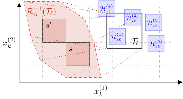
Figure 3: Action $a_{\ell}$ to target set $\mathcal{T}_{\ell}$ is enabled in states $s,s^{\prime}\in S$, as their regions are contained in the backward reachable set $\mathcal{R}^{-1}_{\hat{\alpha}}(\mathcal{T}_{\ell})$. The successor state sets $\mathcal{H}_{i\ell}^{(1)},\ldots,\mathcal{H}_{i\ell}^{(5)}$ for five noise samples, overapproximated as boxes, are shown in blue.

Computing backward reachable sets.

To apply Def. 5, we must compute $\mathcal{R}^{-1}_{\hat{\alpha}}(\mathcal{T}_{\ell})$ for each action $a_{\ell}\in Act$ with associated target set $\mathcal{T}_{\ell}$. Lemma 3, which is stated in Appendix A for brevity, shows that $\mathcal{R}^{-1}_{\hat{\alpha}}(\mathcal{T}_{\ell})$ is a polytope characterized by the vertices of $\mathcal{U}$ and $\mathcal{T}_{\ell}$, which is computationally tractable to compute.

Transition Probability Intervals

We wish to compute the probability $P(s_{i},a_{\ell})(s_{j})$ that taking action $a_{\ell}\in Act$ in a continuous state $x_{k}\in\mathcal{P}_{i}$ yields a successor state $x_{k+1}\in\mathcal{P}_{j}$ that belongs to state $s_{j}\in S$. This conditional probability is defined using Eq. 5 as

$$P(s_{i},a_{\ell})(s_{j}) =\amsmathbb{P}\{x_{k+1}\in\mathcal{P}_{j}\mid a_{\ell}\in Act_{\hat{\alpha}}(s_{i})\}.$$ (9)

Note the outcome of an action $a_{\ell}$ is the same for any origin state $s_{i}$ in which $a_{\ell}$ is enabled. In the remainder, we thus drop the conditioning on $a_{\ell}\in Act_{\hat{\alpha}}(s_{i})$ in Eq. 9 for brevity.

Two factors prevent us from computing Eq. 9: 1) the nominal successor state $\hat{x}_{k+1}$ and the term $\delta(\alpha,x_{k},u_{k})$ are nondeterministic, and 2) the distribution of the noise $\eta_{k}$ is unknown. We deal with the former in the following paragraph while addressing the stochastic noise in Sect. 4.

Capturing nondeterminism.

As a key step, we capture the nondeterminism caused by epistemic uncertainty. First, recall that by construction, we have $\hat{x}_{k+1}\in\mathcal{T}_{\ell}$. Second, we write the set $\Delta_{i}$ of all possible epistemic errors in Eq. 6 as

$$\Delta_{i}=\{\delta(\alpha,x_{k},u_{k})\colon\alpha\in\Gamma,x_{k}\in\mathcal{P}_{i},u_{k}\in\mathcal{U}\}.$$ (10)

Based on these observations, we obtain that the successor state $x_{k+1}$ is an element of a set that we denote by $\mathcal{H}_{i\ell}$:

$$x_{k+1}\in\mathcal{T}_{\ell}+\Delta_{i}+\eta_{k}=\mathcal{H}_{i\ell}.$$ (11)

Crucially, we show in Lemma 4 (provided in Appendix A for brevity) that we can compute an overapproximation of $\Delta_{i}$ based on sets $\mathcal{P}_{i}$ and $\mathcal{U}$, and the model dynamics. Based on the set $\mathcal{H}_{i\ell}$, we bound the probability in Eq. 9 as follows:

Both inequalities follow directly by definition of Eq. 11. The lower bound holds, since if $\mathcal{H}_{i\ell}\subseteq\mathcal{P}_{j}$, then $x_{k+1}\in\mathcal{P}_{j}$ for any $x_{k+1}\in\mathcal{H}_{i\ell}$. The upper bound holds, since by Eq. 11 we have that $x_{k+1}\in\mathcal{H}_{i\ell}$, and thus, if $x_{k+1}\in\mathcal{P}_{j}$, then the intersection $\mathcal{H}_{i\ell}\cap\mathcal{P}_{j}$ must be nonempty.

4 PAC Probability Intervals via Sampling

The interval in Eq. 12 still depends on the noise $\eta_{k}$, whose density function is unknown. We show how to compute PAC bounds on this interval, by sampling a set of $N\in\amsmathbb{N}$ samples of the noise, denoted by $\eta_{k}^{(1)},\ldots,\eta_{k}^{(N)}$. Recall from Assumption 1 that these sample are i.i.d. elements from $(\Omega,\mathcal{F},\amsmathbb{P})$. Each sample $\eta_{k}^{(\iota)}$ yields a set $\mathcal{H}_{i\ell}^{(\iota)}$ (see Fig. 3) that contains the successor state under that value of the noise, i.e.,

$$x_{k+1}^{(\iota)}\in\mathcal{T}_{\ell}+\Delta_{i}+\eta^{(\iota)}_{k}=\mathcal{H}_{i\ell}^{(\iota)}.$$ (13)

For reasons of computational performance, we overapproximate each set $\mathcal{H}_{i\ell}^{(\iota)}$ as the smallest hyperrectangle in $\amsmathbb{R}^{n}$, by taking the point-wise min. and max. over the vertices of $\mathcal{H}_{i\ell}^{(\iota)}$.

Lower Bounds from the Scenario Approach

We interpret the lower bound in Eq. 12 within the sampling-and-discarding scenario approach (Campi and Garatti 2011). Concretely, let $R\subseteq\{1,\ldots,N\}$ be a subset of the noise samples and consider the following convex program:

$$\begin{split}\mathfrak{L}_{R}\colon\operatorname*{minimize}_{\lambda\geq 0}&\enskip\lambda\\ \mathrm{subject~{}to}&\enskip\mathcal{H}_{i\ell}^{(\iota)}\subseteq\mathcal{P}_{j}(\lambda)\,\,\quad\forall\iota\in R,\end{split}$$ (14)

where $\mathcal{P}_{j}(\lambda)$ is a version of $\mathcal{P}_{j}$ scaled by a factor $\lambda$ around an arbitrary point $x\in\mathcal{P}_{j}$, such that $\mathcal{P}_{j}(0)=x$, and $\mathcal{P}_{j}(\lambda_{1})<\mathcal{P}_{j}(\lambda_{2})$ for $\lambda_{1}<\lambda_{2}$; see Badings et al. (2022, Appendix A) for details. The optimal solution $\lambda^{\star}_{R}$ to $\mathfrak{L}_{R}$ results in a region $\mathcal{P}_{j}(\lambda^{\star}_{R})$ such that, for all $\iota\in R$, the set $\mathcal{H}_{i\ell}^{(\iota)}$ for noise sample $\eta_{k}^{(\iota)}$ is contained in $\mathcal{P}_{j}(\lambda^{\star}_{R})$. We ensure that $\mathcal{P}_{j}(\lambda^{\star}_{R})\subseteq\mathcal{P}_{j}$, by choosing $R$ as the set of samples being a subset of $\mathcal{P}_{j}$, i.e.,

$$R\coloneqq\big{\{}\iota\in\{1,\ldots,N\}\colon\mathcal{H}_{i\ell}^{(\iota)}\subseteq\mathcal{P}_{j}\big{\}},$$ (15)

We use the results in Romao, Papachristodoulou, and Margellos (2022, Theorem 5) to lower bound the probability that a random sample $\eta_{k}\in\Omega$ yields $\mathcal{H}_{i\ell}\subseteq\mathcal{P}_{j}(\lambda^{\star}_{R})$. This leads to the following lower bound on the transition probability:

Lemma 1.

Fix a region $\mathcal{P}_{j}$ and confidence probability $\beta\in(0,1)$. Given sets $(\mathcal{H}_{i\ell}^{(\iota)})_{\iota=1}^{N}$, compute $R$. Then, it holds that

$$\amsmathbb{P}^{N}\Big{\{}\amsmathbb{P}\{\eta_{k}\in\Omega\colon\mathcal{H}_{i\ell}\subseteq\mathcal{P}_{j}\}\geq\underaccent{\bar}{p}\Big{\}}\geq 1-\beta,$$ (16)

where $\underaccent{\bar}{p}=0$ if $|R|=0$, and otherwise, $\underaccent{\bar}{p}$ is the solution to

$$\frac{\beta}{N}=\sum\nolimits_{i=0}^{N-|R|}\binom{N}{i}(1-\underaccent{\bar}{p})^{i}\underaccent{\bar}{p}^{N-i}.$$ (17)

More details and the proof of Lemma 1 are in Appendix A.

Upper Bounds via Hoeffding’s Inequality

The scenario approach might lead to conservative estimates of the upper bound in Eq. 12; see Appendix A for details. Thus, we instead apply Hoeffding’s inequality (Boucheron, Lugosi, and Massart 2013) to infer an upper bound $\bar{p}$ of the probability $\amsmathbb{P}\{\mathcal{H}_{i\ell}\cap\mathcal{P}_{j}\neq\emptyset\}$. Concretely, this probability describes the parameter of a Bernoulli random variable, which has value $1$ if $\mathcal{H}_{i\ell}\cap\mathcal{P}_{j}\neq\emptyset$ and $0$ otherwise. The sample sum $\tilde{R}$ of this random variable is given by the number of sets $\mathcal{H}_{i\ell}^{(\iota)}$ that intersect with region $\mathcal{P}_{j}$, i.e.,

$$\tilde{R}\coloneqq\big{\{}\iota\in\{1,\ldots,N\}\colon\mathcal{H}_{i\ell}^{(\iota)}\cap\mathcal{P}_{j}\neq\emptyset\big{\}}.$$ (18)

Using Hoeffding’s inequality, we state the following lemma to bound the upper bound transition probability in Eq. 12.

Lemma 2.

Fix region $\mathcal{P}_{j}$ and confidence probability $\beta\in(0,1)$. Given sets $(\mathcal{H}_{i\ell}^{(\iota)})_{\iota=1}^{N}$, compute $\tilde{R}$. Then, it holds that

$$\amsmathbb{P}^{N}\Big{\{}\amsmathbb{P}\{\eta_{k}\in\Omega\colon\mathcal{H}_{i\ell}\cap\mathcal{P}_{j}\neq\emptyset\}\leq\bar{p}\Big{\}}\geq 1-\beta,$$ (19)

where the upper bound $\bar{p}$ is computed as

$$\bar{p}=\min\left\{1,\enskip\frac{\tilde{R}}{N}+\sqrt{\frac{1}{2N}\log\Big{(}\frac{1}{\beta}\Big{)}}\right\}.$$ (20)

More details and the proof of Lemma 2 are in Appendix A.

Probability Intervals with PAC Guarantees

We apply Lemmas 1 and 2 as follows to compute a PAC probability interval for a specific transition of the iMDP.

Theorem 1 (PAC probability interval).

Fix a region $\mathcal{P}_{j}$ and a confidence probability $\beta\in(0,1)$. For the collection $(\mathcal{H}_{i\ell}^{(\iota)})_{\iota=1}^{N}$, compute $\underaccent{\bar}{p}$ and $\bar{p}$ using Lemmas 1 and 2. Then, the transition probability $P(s_{i},a_{\ell})(s_{j})$ is bounded by

$$\amsmathbb{P}^{N}\Big{\{}\underaccent{\bar}{p}\leq P(s_{i},a_{\ell})(s_{j})\leq\bar{p}\Big{\}}\geq 1-2\beta.$$ (21)

Proof.

Theorem 1 follows directly by combining Lemmas 1 and 2 via the union bound with the probability interval in Eq. 12, which asserts that these bounds are both correct with a probability of at least $1-2\beta$. ∎

Counting samples.

The inputs to Theorem 1 are the sample counts $R$ (fully contained in $\mathcal{P}_{j}$) and $\tilde{R}$ (at least partially contained in $\mathcal{P}_{j}$), and the confidence probability $\beta$. Thus, the problem of computing probability intervals reduces to a counting problem on the samples. In Appendix B, we describe a procedure that significantly speeds up this counting process in a sound way by merging (and overapproximating) sets $\mathcal{H}^{(\iota)}$ that are very similar.

Figure 4: Our overall approach to solve the formal problem based on the abstraction method outlined in Sects. 3 and 4.

5 Overall Abstraction Method

We provide an algorithm to solve the formal problem based on the proposed abstraction method. The approach is shown in Fig. 4 and consists of an offline planning phase, in which we create the iMDP and compute a robust optimal policy, and an online control phase in which we automatically derive a provably-correct controller for the continuous model.

1) Create abstraction.

Given a model as in Eq. 1, a partition $(\mathcal{P}_{i})_{i=1}^{L}$ of the state space as defined by Def. 4, and a confidence level $\beta\in(0,1)$ as inputs, we create an abstract iMDP by applying the techniques presented in Sects. 3 and 4.

2) Compute robust optimal policy.

We compute a robust optimal policy $\pi^{\star}$ for the iMDP using Eq. 3. Recall that the problem is to find a controller together with a lower bound $\lambda$ on the reach-avoid probability. If this condition holds, we output the policy and proceed to step 3; otherwise, we attempt to improve the abstraction in one of the following ways.

First, we can refine the partition at the cost of a larger iMDP, as shown in Sect. 6. Second, using more samples $N$ yields an improved iMDP through tighter intervals (see, e.g., Badings et al. (2022) for such trade-offs). Finally, the uncertainty in $\alpha\in\Gamma$ may be too large, meaning we need to reduce set $\Gamma$ using learning techniques (see the related work).

3) Online control.

The stored policy is a time-varying map from iMDP states to actions. Recall that an action $a_{\ell}\in Act$ corresponds to applying a control $u_{k}$ such that the nominal state $\hat{x}_{k+1}\in\mathcal{T}_{\ell}$. In view of Eq. 4 and Def. 5, such a $u_{k}\in\mathcal{U}$ for the original model exists by construction and is obtained as the solution to the following convex optimization program:

$$\begin{split}c_{\ell}(x_{k})=&\operatorname*{arg\,min}_{u\in\mathcal{U}}\quad\|A(\hat{\alpha})x_{k}+B(\hat{\alpha})u-\tilde{t}_{\ell}\|_{2}\\ &\text{subject to}\quad A(\hat{\alpha})x_{k}+B(\hat{\alpha})u\in\mathcal{T}_{\ell},\end{split}$$ (22)

with $\tilde{t}_{\ell}\in\mathcal{T}_{\ell}$ a representative point, which indicates a point to which we want to steer the nominal state (in practice, we choose $\tilde{t}_{\ell}$ as the center of $\mathcal{T}_{\ell}$, but the theory holds for any such point). Thus, upon observing the current continuous state $x_{k}$, we determine the optimal action $a_{\ell}$ in the corresponding iMDP state and apply the control input $u_{k}=c_{\ell}(x_{k})\in\mathcal{U}$.

Correctness of the Abstraction

We lift the confidence probabilities on individual transitions obtained from Theorem 1 to a correctness guarantee on the whole iMDP. The following theorem states this key result:

Theorem 2 (Correctness of the iMDP).

Generate an iMDP abstraction $\mathcal{M}{I}$ and compute the robust reach-avoid probability $\underline{Pr}^{\pi^{\star}}(\mathcal{M}{I}\models\varphi_{s_{I}}^{K})$ under optimal policy $\pi^{\star}$. Under the controller $c$ defined by Eq. 22 for each $k\leq K$, it holds that

$$\amsmathbb{P}\left\{V(x_{0},\alpha,c)\geq\underline{Pr}^{\pi^{\star}}(\mathcal{M}{I}\models\varphi_{s_{I}}^{K})\right\}\geq 1-2\beta LM.$$ (23)

The proof of Theorem 2, which we provide in Appendix A, uses the union bound with the fact that the iMDP has at most $LM$ unique probability intervals. By tuning $\beta\in(0,1)$, we thus obtain an abstraction that is correct with a user-specified confidence level of $1-\tilde{\beta}=1-2\beta LM$.

Crucially, we note that Theorem 2 is, with a probability of at least $1-2\beta LM$, a solution to the formal problem stated in Sect. 2 with threshold $\lambda=\underline{Pr}^{\pi^{\star}}(\mathcal{M}{I}\models\varphi_{s_{I}}^{K})$.

Sample complexity.

The required sample size $N$ depends logarithmically on the confidence level, cf. Lemmas 1 and 2. Moreover, the number of unique intervals is often lower than the worst-case of $LM$, so the bound in Theorem 2 can be conservative. In particular, the number of intervals only depends on the state and action definitions of the iMDP, and is thus observable before we apply Theorem 1. To compute less conservative probability intervals, we replace $LM$ in Eq. 23 with the observed number of unique intervals.

Uncertain Additive Disturbance

We extend the generality of our models with an additive parameter representing an external disturbance $q_{k}\in\mathcal{Q}$ that, in the spirit of this paper, belongs to a convex set $\mathcal{Q}\subset\amsmathbb{R}^{n}$ (Blanchini and Miani 2008). The resulting model is

$$x_{k+1}=A(\alpha)x_{k}+B(\alpha)u_{k}+q_{k}+\eta_{k}.$$ (24)

This additional parameter $q_{k}$ models uncertain disturbances that are not stochastic (and can thus not be captured by $\eta_{k}$), and that are independent of the state $x_{k}$ and control $u_{k}$ (and can thus not be captured in $A(\alpha)$ or $B(\alpha)$). To account for parameter $q_{k}$ (which creates another source of epistemic uncertainty), we expand Eq. 6 and Lemma 4 to be robust against any $q_{k}\in\mathcal{Q}$. While this extension increases the size of the sets $\mathcal{H}_{i\ell}^{(\iota)},\iota=1,\ldots,N$, the procedure outlined in Sect. 4 to compute probability intervals remains the same.

Generality of the model.

The parameter $q_{k}$ expands the applicability of our approach significantly. Consider, e.g., a building temperature control problem, where only the temperatures of adjacent rooms affect each other. We can decompose the model dynamics into the individual rooms by capturing any possible influence between rooms into $q_{k}\in\mathcal{Q}$, as is common in assume-guarantee reasoning (Bobaru, Pasareanu, and Giannakopoulou 2008). We apply this extension to a large building temperature control problem in Sect. 6.

6 Numerical Experiments

We perform experiments to answer the question: “Can our method synthesize controllers that are robust against epistemic uncertainty in parameters?”  In this section, we focus on problems from motion planning and temperature control, and we discuss an additional experiment on a variant of the automated anesthesia delivery benchmark from Abate et al. (2018) in Appendix C. All experiments ran single-threaded on a computer with $32$ $3.7$GHz cores and $64$GB RAM. A Python implementation of our approach is available at https://github.com/LAVA-LAB/DynAbs, using the probabilistic model checker PRISM (Kwiatkowska, Norman, and Parker 2011) to compute optimal iMDP policies.

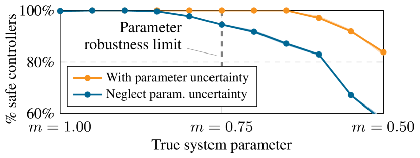
Figure 5: Percentage of initial states with safe performance guarantees (i.e., the simulated reach-avoid probability is above the optimum of Eq. 3 on the iMDP). Our approach that accounts for epistemic uncertainty is 100% safe up to the parameter robustness limit; neglecting uncertainty is not.

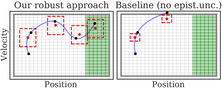
Figure 6: With our approach, the system safely reaches the goal (in green), while the baseline neglecting epistemic uncertainty leaves the safe set (gray box), as it underestimates the successor state sets $\mathcal{H}_{i\ell}$ defined in Eq. 11 (red boxes).

Longitudinal Drone Dynamics

We revisit Example 1 of a drone with an uncertain mass $m\in[0.75,1.25]$. We fix the nominal value of the mass as $\hat{m}=1$. To purely show the effect of epistemic uncertainty, we set the covariance of the aleatoric uncertainty in $\eta_{k}$ (being a Gaussian distribution) to almost zero. The specification is to reach a position of $p_{k}\geq 8$ before time $K=12$, while avoiding speeds of $|v_{k}|\geq 10$. Thus, the safe set is $\mathcal{Z}=[-\infty,\infty]\times[-10,10]$, of which we create a partition covering $\mathcal{X}=[-10,14]\times[-10,10]$ and into $24\times 20$ regions. We use $20$K samples of the noise to estimate probability intervals. We compare against a baseline that builds an iMDP for the nominal model only, thus neglecting parameter uncertainty.

Neglecting epistemic uncertainty is unsafe.

We solve the formal problem stated in Sect. 2 for every initial state $x_{0}\in\mathcal{X}$, resulting in a threshold $\lambda$ for each of those states. The run time for solving this benchmark is around $3\text{\,}\mathrm{s}$. For each $x_{0}$, we say that the controller $c$ at a parameter value $\alpha\in\Gamma$ is unsafe, if the reach-avoid probability $V(x_{0},\alpha,c)$ (estimated using Monte Carlo simulations) is below $\lambda=\underline{Pr}^{\pi^{\star}}(\mathcal{M}{I}\models\varphi_{s_{I}}^{K})$ on the iMDP, as per Eq. 3. In Fig. 5, we show the deviation of the actual mass $m$ from its nominal value, versus the average percentage of states with a safe controller (over 10 repetitions). The parameter robustness limit represents the extreme values of the parameter against which our approach is guaranteed to be robust ($m=0.75$ and $1.25$ in this case).

Our approach yields 100% safe controllers for deviations well over the robustness limit, while the baseline yields 6% unsafe controllers at this limit. We show simulated trajectories under an actual mass $m=0.75$ in Fig. 6. These trajectories confirm that our approach safely reaches the goal region while the baseline does not, as it neglects epistemic uncertainty, which is equivalent to assuming $\Delta_{i}=0$ in Eq. 11.

Multiple uncertain parameters.

To show that our contributions hold independently of the uncertain parameter, we consider a case in which, in addition to the uncertain mass, we have an uncertain friction coefficient. The results of this experiment, presented in Appendix C, show that we obtain controllers with similar correctness guarantees, irrespective of the number of uncertain parameters.

Building Temperature Control

We consider a temperature control problem for a 5-room building with Gaussian process noise, each with a dedicated radiator that has an uncertain power output of $\pm 10\%$ around its nominal value (see Appendix C for modeling details). The $10$D state of this model captures the temperatures of 5 rooms and 5 radiators. The goal is to maintain a temperature within $21\pm$2.5\text{\,}\mathrm{\SIUnitSymbolCelsius}$$ for $15$ steps of $20\text{\,}\mathrm{min}$.

Interactions between rooms as nondeterminism.

Since a direct partitioning of the $10$D state space is infeasible, we use the procedure from Sect. 5 to capture any possible thermodynamic interaction between rooms in the uncertain parameter $q_{k}\in\mathcal{Q}$. In particular, we show in Appendix C that the set $\mathcal{Q}_{i}$ for room $i\in\{1,\ldots,5\}$ is characterized by the maximal temperature difference between room $i$ and all adjacent rooms. For the partition used in this particular reach-avoid problem, this maximal temperature difference is $23.5-18.5=$5\text{\,}\mathrm{\SIUnitSymbolCelsius}$$. Following this procedure, we can easily derive a set-bounded representation of $\mathcal{Q}$, allowing us to decouple the dynamics into the individual rooms.

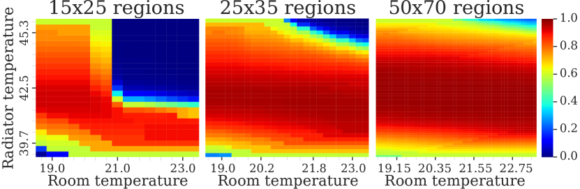
Figure 7: Specification satisfaction probabilities on the iMDP for a single room of the temperature control problem.

Refining partitions improves results.

We apply our method with an increasingly more fine-grained state-space partition. In Fig. 7, we present, for three different partitions, the thresholds $\lambda$ of satisfying the specification under the robust optimal iMDP policy as per Eq. 3, from any initial state $x_{0}\in\mathcal{X}$. These results confirm the idea from Sect. 5 that partition refinement can lead to controllers with better performance guarantees. A more fine-grained partition leads to more actions enabled in the abstraction, which in turn improves the robust lower bound on the reach-avoid probability.

Scalability.

We report run times and model sizes in Table 1 in Appendix C. The run times vary between $5.6\text{\,}\mathrm{s}$ and $8\text{\,}\mathrm{min}$ for the smallest ($15\times 25$) and largest ($70\times 100$) partitions, respectively. Without the decoupling procedure, even a 2-room version on the smallest partition leads to a memory error. By contrast, our approach with decoupling procedure has linear complexity in the number of rooms. We observe that accounting for epistemic uncertainty yields iMDPs with more transitions and slightly higher run times (for the largest partition: $82$ instead of $52$ million transitions and $8$ instead of $5\text{\,}\mathrm{min}$). This is due to larger successor state sets $\mathcal{H}_{i\ell}^{(\iota)}$ in Eq. 11 caused by the epistemic error $\Delta_{i}$.

7 Conclusions and Future Work

We have presented a novel abstraction-based controller synthesis method for dynamical models with aleatoric and epistemic uncertainty. The method captures those different types of uncertainties in order to ensure certifiably safe controllers. Our experiments show that we can synthesize controllers that are robust against uncertainty and, in particular, against deviations in the model parameters.

Generality of our approach.

We stress that the models in Eqs. 1 and 24 can capture many common sources of uncertainty. As we have shown, our approach simultaneously deals with epistemic uncertainty over one or multiple parameters, as well as aleatoric uncertainty due to stochastic noise of an unknown distribution. Moreover, the additive parameter $q_{k}$ introduced in Sect. 5 enables us to generate abstractions that faithfully capture any error term represented by a bounded set (as we have done for the temperature control problem). For example, we plan to apply our method to nonlinear systems, such as non-holonomic robots (Thrun, Burgard, and Fox 2005). Concretely, we may apply our abstraction method on a linearized version of the system while treating linearization errors as nondeterministic disturbances $q_{k}\in\mathcal{Q}$ in Eq. 24. The main challenge is then to obtain this set-bounded representation $\mathcal{Q}$ of the linearization error.

Scalability.

Enforcing robustness against epistemic uncertainty hampers the scalability of our approach, especially compared to similar non-robust abstraction methods, such as Badings et al. 2022. To reduce the computational complexity, we restrict partitions to be rectangular, but the theory is valid for any convex partition. A finer partition yields larger iMDPs but also improves the guarantees on controllers.

Safe learning.

Finally, we wish to integrate the abstractions in a safe learning framework (Brunke et al. 2022) by, as discussed in the related work in Sect. 1, applying our approach to guarantee safe interactions with the system.

Appendix A Proofs

Computing Backward Reachable Sets

The following lemma shows that computing backward reachable sets, as required for Def. 5 is computationally tractable. Because $\mathcal{T}_{\ell}$ and $\mathcal{U}$ are convex polytopes, the inverse of the dynamics of the nominal model in Eq. 4 is also a convex polytope, which is exactly characterized by the vertices of $\mathcal{U}$ and $\mathcal{T}_{\ell}$. We formalize this claim in Lemma 3.

Lemma 3 (Representation of the backward reachable set).

Let the control space $\mathcal{U}=\mathrm{conv}(u^{1},\ldots,u^{q}),\,q\in\amsmathbb{N}$, and target set $\mathcal{T}_{\ell}=\mathrm{conv}(t^{1},\ldots,t^{d}),\,d\in\amsmathbb{N}$, of action $a_{\ell}$ be given in their vertex representations. Under Assumption 2, we have that

$$\mathcal{R}^{-1}_{\hat{\alpha}}(\mathcal{T}_{\ell})=\mathrm{conv}(\bar{x}_{ij}\colon i=1,\ldots,d,~{}j=1,\ldots,q),$$ (25)

where $\bar{x}_{ij}$ is the unique solution of the linear system

$$A(\hat{\alpha})\bar{x}_{ij}+B(\hat{\alpha})u^{j}=t^{i}.$$ (26)

Proof.

We first proof that Eq. 25 holds with inclusion, i.e.,

$$\mathrm{conv}(\bar{x}_{ij}\colon i=1,\ldots,d,~{}j=1,\ldots,q)\subseteq\mathcal{R}^{-1}_{\hat{\alpha}}(\mathcal{T}_{\ell}).$$ (27)

Let $z$ be any element belonging to the right-hand side of Eq. 25, i.e. $z\in\mathrm{conv}(\bar{x}_{ij}\colon i=1,\ldots,d,~{}j=1,\ldots,q)$. Then, there exists $\gamma_{ij}$, $i=1,\ldots,d,j=1,\ldots,q$, such that

$$\gamma_{ij}\geq 0,\quad\sum_{i,j=1}^{d,q}\gamma_{ij}=1,\quad z=\sum_{i,j=1}^{d,q}\gamma_{ij}\bar{x}_{ij}.$$

For each vertex $u^{j}$ of $\mathcal{U}$, $j=1\ldots,q$, let $\xi_{j}=\sum_{i=1}^{d}\gamma_{ij}$ and write the control input $u$ corresponding to point $z$:

$$u=\sum_{j=1}^{q}\xi_{j}u^{j},\quad u\in\mathcal{U},$$

which is admissible by construction. Now, note that the mapping of the pair $(z,u)$ under the dynamics satisfies

$$A(\hat{\alpha})z+B(\hat{\alpha})u =\sum_{i,j=1}^{d,q}\gamma_{ij}A(\hat{\alpha})\bar{x}_{ij}+\sum_{j=1}^{q}\xi_{j}B(\hat{\alpha})u^{j}$$

$$=\sum_{i,j=1}^{d,q}\gamma_{ij}\left(A(\hat{\alpha})\bar{x}_{ij}+B(\hat{\alpha})u^{j}\right)$$

$$=\sum_{i=1}^{d}\bar{\gamma}_{i}t^{i}\in\mathcal{T}_{\ell},$$

where the first equality follows from the definition of $z$ and $u$, the second by the definition of $\xi_{j}=\sum_{i=1}^{d}\gamma_{ij}$, and the third by letting $\bar{\gamma}_{i}=\sum_{j=1}^{q}\gamma_{ij}$ and noting that $\sum_{i=1}^{d}\bar{\gamma}_{i}=1$ and $\bar{\gamma}_{i}\geq 0$ for all $i=1,\ldots,d$. In other words, the mapping of the pair $(z,u)$ belongs to the target set $\mathcal{T}_{\ell}$, which implies that Eq. 27 holds by construction. This concludes the first part of the lemma.

To show the opposite direction in Eq. 25, let $z$ be any element in $\mathcal{R}^{-1}_{\hat{\alpha}}(\mathcal{T}_{\ell})$. By definition of the backward reachable set (see Sect. 3), this means that there exist $\xi_{j}\geq 0$ and $\gamma_{i}\geq 0$, $i=1,\ldots,d,j=1,\ldots,q$, with $\sum_{j=1}^{q}\xi_{j}=1$ and $\sum_{i=1}^{d}\gamma_{i}=1$, such that

$$A(\hat{\alpha})z+B(\hat{\alpha})\left(\sum_{j=1}^{q}\xi_{j}u^{j}\right)=\sum_{i=1}^{d}\gamma_{i}t^{i}.$$ (28)

In other words, if $z\in\mathcal{R}^{-1}_{\hat{\alpha}}(\mathcal{T}_{\ell})$ then there exists an input $u\in\mathcal{U}$ such that $A(\hat{\alpha})z+B(\hat{\alpha})u\in\mathcal{T}_{\ell}$. Substituting (26) into (28) we obtain

$$\begin{split}&A(\hat{\alpha})z+B(\hat{\alpha})\sum_{j=1}^{q}\xi_{j}u^{j}=\sum_{i=1}^{d}\gamma_{i}\left(A(\hat{\alpha})\bar{x}_{ik}+B(\hat{\alpha})u^{k}\right)\\ &A(\hat{\alpha})z=\sum_{i=1}^{d}\gamma_{i}\left(A(\hat{\alpha})\bar{x}_{ik}+B(\hat{\alpha})u^{k}\right)-B(\hat{\alpha})\sum_{j=1}^{q}\xi_{j}u^{j},\end{split}$$ (29)

for all $k=1,\ldots,q$. Multiplying both sides of (29) by $A(\hat{\alpha})^{-1}$, which is allowed due to Assumption 2, yields

$$\begin{split}z=\sum_{i=1}^{d}\gamma_{i}\big{(}\bar{x}_{ik}&+A(\hat{\alpha})^{-1}B(\hat{\alpha})u^{k}\big{)}\\ &-A(\hat{\alpha})^{-1}B(\hat{\alpha})\sum_{j=1}^{q}\xi_{j}u^{j}.\end{split}$$ (30)

Since Eq. 30 holds for all $k=1,\ldots,q$, we can multiply both sides by $\xi_{k}$ for each $k=1,\ldots,q$, and sum up the resulting expression. Due to the fact that $\sum_{k=1}^{q}\xi_{k}=1$, we obtain

$$\begin{split}z=\sum_{i,k=1}^{d,q}\bar{\gamma}_{ik}\bar{x}_{ik}&+A(\hat{\alpha})^{-1}B(\hat{\alpha})\sum_{k=1}^{q}\xi_{k}u^{k}\\ &-A(\hat{\alpha})^{-1}B(\hat{\alpha})\sum_{j=1}^{q}\xi_{j}u^{j},\end{split}$$ (31)

where $\bar{\gamma}_{ik}=\xi_{k}\gamma_{i}$, which is larger than or equal to zero for all $i=1,\ldots,d,k=1,\ldots,q$. Since the last two terms on the right-hand side of (31) cancel out and $\sum_{i,k=1}^{d,q}\bar{\gamma}_{ik}=1$, we conclude that $z\in\mathrm{conv}(\bar{x}_{ij}:i=1,\ldots,d,j=1,\ldots,q)$, thus proving the opposite inclusion and concluding the proof of the lemma. ∎

Bounding the Epistemic Error

The following lemma shows that the set $\Delta_{i}$, defined in Eq. 10 is a subset of a convex polytope, which is characterized by the region $\mathcal{P}_{i}$, the feasible control space $\mathcal{U}$, and the model dynamics. Importantly, note that the probability interval in Eq. 12 also holds for any overapproximation of $\Delta_{i}$ obtained using Lemma 4.

Lemma 4.

Given the vertex representations of sets $\mathcal{P}_{i}=\mathrm{conv}(v^{1},\ldots,v^{p})$ and $\mathcal{U}=\mathrm{conv}(u^{1},\ldots,u^{q})$ for $p,q\in\amsmathbb{N}$, define $\Delta_{i}$ as in Eq. 10. Then, we have that

$$\begin{split}\Delta_{i}\subseteq\mathrm{conv}\Big{(}&\big{(}A_{\iota}-A(\hat{\alpha})\big{)}v^{j}+\big{(}B_{\iota}-B(\hat{\alpha})\big{)}u^{\ell}\\ &\colon\iota,j,\ell=1,\ldots,\{r,p,q\}\Big{)},\end{split}$$ (32)

where $A_{1},\ldots,A_{r}$ and $B_{1},\ldots,B_{r}$ are defined in Eq. 2.

Proof.

First, let us fix any $\alpha\in\Gamma$, and observe that the set $\Delta_{i}$ defined in Eq. 10 evaluated at $\alpha$ is written as

$$\begin{split}\Delta_{i}(\alpha)&=\left\{\delta(\alpha,x_{k},u_{k})\colon x_{k}\in\mathcal{P}_{i},u_{k}\in\mathcal{U}\right\}\\ &=\Big{\{}(A(\alpha)-A(\hat{\alpha}))x_{k}+(B(\alpha)-B(\hat{\alpha}))u_{k}\\ &\quad\quad\colon x_{k}\in\mathcal{P}_{i},u_{k}\in\mathcal{U}\Big{\}}.\end{split}$$ (33)

We observe that the sets $\{(A(\alpha)-A(\hat{\alpha}))x_{k}\colon x_{k}\in\mathcal{P}_{i}\}$ and $\{(B(\alpha)-B(\hat{\alpha}))u_{k}\colon u_{k}\in\mathcal{U}\}$ are both convex polytopes characterized by the vertices of $\mathcal{P}_{i}$ and $\mathcal{U}$, respectively. Thus, we rewrite Eq. 33 as

$$\begin{split}\Delta_{i}(\alpha)=\mathrm{conv}\Big{(}&(A(\alpha)-A(\hat{\alpha}))v^{j}+(B(\alpha)-B(\hat{\alpha}))u^{\ell}\\ &\enskip\colon j,\ell=1,\ldots,\{p,q\}\Big{)}.\end{split}$$

Note that the full set $\Delta_{i}$ is the union of $\Delta_{i}(\alpha)$ over all $\alpha\in\Gamma$:

$$\begin{split}\Delta_{i}&=\bigcup_{\alpha\in\Gamma}\Delta_{i}(\alpha)\\ &\subseteq\mathrm{conv}\Big{(}(A(\alpha)-A(\hat{\alpha}))v^{j}+(B(\alpha)-B(\hat{\alpha}))u^{\ell}\\ &\qquad\qquad\enskip\colon j,\ell=1,\ldots,\{p,q\},\,\alpha\in\Gamma\Big{)}.\end{split}$$ (34)

Crucially, observe that for any fixed pair of vertices $\bar{v}\coloneqq v^{j}$ and $\bar{u}\coloneqq u^{\ell}$, $j,\ell=1,\ldots,\{p,q\}$, we can write the convex hull in Eq. 34 in terms of only the matrices $A_{\iota},B_{\iota}$ for $\iota=1,\ldots,r$ of which $A(\alpha)$ and $B(\alpha$ are a convex combination (as defined in Eq. 2):

$$\mathrm{conv}\big{(}(A(\alpha)-A(\hat{\alpha}))\bar{v}+(B(\alpha)-B(\hat{\alpha}))\bar{u}\colon\alpha\in\Gamma\big{)}$$

$$\enskip=\mathrm{conv}\Big{(}(A(\alpha)-A(\hat{\alpha}))\bar{v}+(B(\alpha)-B(\hat{\alpha}))\bar{u}$$

$$\qquad\qquad\quad\colon\alpha=e_{1},\ldots,e_{r}\Big{)}$$ (35)

$$\enskip=\mathrm{conv}\big{(}(A_{\iota}-A(\hat{\alpha}))\bar{v}+(B_{\iota}-B(\hat{\alpha}))\bar{u}\colon\iota=1,\ldots,r\big{)},$$

where $e_{\iota}\in\amsmathbb{R}^{r}$ is the vector with all components equal to $0$, except the $\iota^{\text{th}}$, which is $1$. The last equality in Eq. 35 holds, since $A(e_{\iota})=A_{\iota}$ and $B(e_{\iota})=B_{\iota}$ for any $\iota=1\ldots,r$. In other words, considering the values $\alpha\in\Gamma\setminus\{e_{1},\ldots,e_{r}\}$ in Eq. 34 is redundant since these values can be expressed as a convex combination of $\alpha\in\{e_{1},\ldots,e_{r}\}$, as in Eq. 35. As a result, we simplify Eq. 34 as

$$\begin{split}\Delta_{i}\subseteq\mathrm{conv}\Big{(}&\big{(}A_{\iota}-A(\hat{\alpha})\big{)}v^{j}+\big{(}B_{\iota}-B(\hat{\alpha})\big{)}u^{\ell}\\ &\colon\iota,j,\ell=1,\ldots,\{r,p,q\}\Big{)},\end{split}$$

which equals Eq. 32. This concludes the proof of Lemma 4. ∎

Eq. 32 does not hold with equality.

It may be tempting to conclude that Eq. 32 holds with equality. However, we show with a simple example that this is not the case. Specifically, we apply Lemma 4 to a model with the matrices

$$\begin{split}A_{1}&=\begin{bmatrix}0.9&1\\ 0&0.9\end{bmatrix},\,A_{2}=\begin{bmatrix}1.1&1\\ 0&1.1\end{bmatrix},\,A(\hat{\alpha})=\begin{bmatrix}1&1\\ 0&1\end{bmatrix},\\ B_{1}&=B_{2}=B(\hat{\alpha})=\begin{bmatrix}1\\ 1\end{bmatrix},\,\,\mathcal{P}_{i}=[0,1]^{2},\,\,\mathcal{U}=[-5,5].\end{split}$$

The resulting right-hand side of Eq. 32 is shown by the dashed hull in Fig. 8. Moreover, to approximate $\Delta_{i}$, we compute $\delta(\alpha,x_{k},u_{k})$ for many linearly spaced points $\alpha\in\Gamma$, $x_{k}\in\mathcal{P}_{i}$, and $u_{k}\in\mathcal{U}$, which are shown by the blue dots in Eq. 32. While the convex hull is a sound overapproximation of the set $\Delta_{i}$, the opposite is clearly not the case (there are points in the convex hull that are not included in $\Delta_{i}$). This result empirically shows that Eq. 32 of Lemma 4 does not hold with equality.

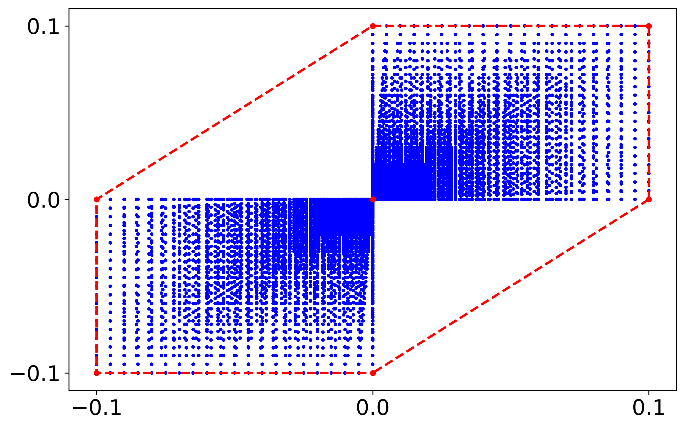
Figure 8: Overapproximation of set $\Delta_{i}$ using Lemma 4, shown as the red dashed convex hull, and many points in the set $\Delta_{i}$ for different $x_{k}\in\mathcal{P}_{i}$ and $u_{k}\in\mathcal{U}$, shown in blue.

Proof of Lemma 1 (Lower Bound Probability)

Our goal is to show that if we remove $R$ samples as defined in Eq. 15, the optimal solution to the scenario optimization problem $\mathfrak{L}_{R}$ satisfies the claim in Lemma 1. To this end, we use the key result from Romao, Margellos, and Papachristodoulou (2020, Theorem 5), which requires three key assumptions on the scenario problem $\mathfrak{L}_{R}$:

1. Problem $\mathfrak{L}_{R}$ belongs to the class of so-called fully-supported problems (see Campi and Garatti (2008) for a definition);

2. The solution to problem $\mathfrak{L}_{R}$ is unique;

3. All samples not contained in $R$ violate the optimal solution with probability one.

Requirement (1) is satisfied because problem $\mathfrak{L}_{R}$ has a scalar decision variable, (2) is satisfied due to Assumption 1, and (3) is satisfied by definition of $R$, since any sample not contained in $R$ is violated by the solution to $\mathfrak{L}_{R}$ with probability one. We invoke the key result by Romao, Margellos, and Papachristodoulou (2020, Theorem 5) that, under these requirements, the optimal solution $\lambda^{\star}_{R}$ satisfies the following:

$$\begin{split}\amsmathbb{P}^{N}\Big{\{}&\amsmathbb{P}\{\eta_{k}\in\Omega\colon\mathcal{H}_{i\ell}\not\subseteq\mathcal{P}_{j}(\lambda^{\star}_{R})\}\leq\varepsilon\Big{\}}\\ &\qquad=1-\sum_{i=0}^{N-|R|}\binom{N}{i}\varepsilon^{i}(1-\varepsilon)^{N-i},\end{split}$$ (36)

where $\varepsilon$ is an upper bound on the so-called violation probability, which is the probability that a sample $\mathcal{H}_{i\ell}$ under a random noise value $\eta_{k}\in\Omega$ is not fully contained in the feasible set $\mathcal{P}_{j}(\lambda^{\star}_{R})$ to problem $\mathfrak{L}_{R}$. Intuitively, Eq. 36 states that the violation probability is bounded by $\varepsilon$, and this result holds with the confidence at the right-hand side. Note that we can rewrite this violation probability as the satisfaction probability as:

$$\amsmathbb{P}\{\mathcal{H}_{i\ell}\not\subseteq\mathcal{P}_{j}(\lambda^{\star}_{R})\}=1-\amsmathbb{P}\{\mathcal{H}_{i\ell}\subseteq\mathcal{P}_{j}(\lambda^{\star}_{R})\}.$$

Moreover, by defining $\underaccent{\bar}{p}=1-\varepsilon$, we rewrite Eq. 36 as

$$\begin{split}\amsmathbb{P}^{N}\Big{\{}&1-\amsmathbb{P}\{\eta_{k}\in\Omega\colon\mathcal{H}_{i\ell}\subseteq\mathcal{P}_{j}(\lambda^{\star}_{R})\}\leq 1-\underaccent{\bar}{p}\Big{\}}\\ &=\amsmathbb{P}^{N}\Big{\{}\amsmathbb{P}\{\eta_{k}\in\Omega\colon\mathcal{H}_{i\ell}\subseteq\mathcal{P}_{j}(\lambda^{\star}_{R})\}\geq\underaccent{\bar}{p}\Big{\}}\\ &=1-\sum_{i=0}^{N-|R|}\binom{N}{i}(1-\underaccent{\bar}{p})^{i}\underaccent{\bar}{p}^{N-i}=1-\frac{\beta}{N}.\end{split}$$ (37)

We will motivate our choice of $1-\frac{\beta}{N}$ in Eq. 37 below. To proof Lemma 1, we need to show that for some $R$, it holds that $\mathcal{P}_{j}(\lambda^{\star}_{R})\subseteq\mathcal{P}_{j}$. However, we do not know a priori (i.e., before observing the samples) for which set $R$ this claim holds. Specifically, there are $N$ possible sets $R$ that we may consider, ranging from sizes $|R|\in\{1,\ldots,N\}$. Let us, for each value of $|R|$, denote by $\mathcal{A}_{|R|}$ the event that

$$\amsmathbb{P}\{\eta_{k}\in\Omega\colon\mathcal{H}_{i\ell}\subseteq\mathcal{P}_{j}(\lambda^{\star}_{R})\}\geq\underaccent{\bar}{p}.$$

From Eq. 37, we have that $\amsmathbb{P}\{\mathcal{A}_{|R|}\}=1-\frac{\beta}{N}$, while for its complement $\mathcal{A}^{\prime}_{|R|}$ we obtain $\amsmathbb{P}\{\mathcal{A}^{\prime}_{|R|}\}=\frac{\beta}{N}$. Via Boole’s inequality (the union bound), we know that

$$\amsmathbb{P}^{N}\Big{\{}\bigcap_{\xi=1}^{N}\mathcal{A}_{\xi}\Big{\}}=1-\amsmathbb{P}^{N}\Big{\{}\bigcup_{\xi=1}^{N}\mathcal{A}^{\prime}_{\xi}\Big{\}}\geq 1-\beta.$$ (38)

After observing the samples at hand, we determine $R$ as per Eq. 15, giving an expression in the form of Eq. 37 for that set $R$. The probability that this expression holds cannot be smaller than that of the intersection of all events in Eq. 38. Thus, we obtain that

$$\amsmathbb{P}^{N}\Big{\{}\amsmathbb{P}\{\eta_{k}\in\Omega\colon\mathcal{H}_{i\ell}\subseteq\mathcal{P}_{j}\}\geq\underaccent{\bar}{p}\Big{\}}\geq 1-\beta,$$ (39)

where $\underaccent{\bar}{p}=0$ if $R=\emptyset$, i.e., $|R|=0$ (which trivially holds with probability one), and otherwise, $\underaccent{\bar}{p}$ is the solution to Eq. 37 for that cardinality $|R|$:

$$\frac{\beta}{N}=\sum_{i=0}^{N-|R|}\binom{N}{i}(1-\underaccent{\bar}{p})^{i}\underaccent{\bar}{p}^{N-i},$$ (40)

which is equivalent to Eqs. 16 and 17. Thus, we conclude the proof.

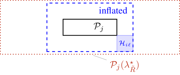
Figure 9: Visualization of Eq. 41, where inflated represented the region $\mathcal{P}_{j}$ inflated by the size of the samples $\mathcal{H}_{i\ell}$ (overapproximated by a box).

Proof of Lemma 2 (Upper Bound Probability)

Before proving Lemma 2, we discuss the claim from Sect. 4 that using scenario optimization may lead to conservative estimates of the upper bound transition probabilities. To use scenario optimization for computing an upper bound probability, we must (analogous to computing a lower bound) find a subset of samples $\tilde{R}\subset\{1,\ldots,N\}$ such that the solution to the scenario problem in Eq. 14 yields a region $\mathcal{P}_{j}(\lambda^{\star}_{\tilde{}R})$ that is (roughly speaking) at least as big as the region $\mathcal{P}_{j}$, inflated by the width of the sample sets $\mathcal{H}_{i\ell}$. The intuition is that, to find a valid upper bound transition probability, we must find a region $\mathcal{P}_{j}(\lambda^{\star}_{\tilde{}R})$ such that if $\mathcal{H}_{i\ell}\not\subseteq\mathcal{P}_{j}(\lambda^{\star}_{\tilde{}R})$, we always have $\mathcal{H}_{i\ell}\cup\mathcal{P}_{j}=\emptyset$. Formally, this condition is written as follows:

$$\mathcal{P}_{j}(\lambda^{\star}_{\tilde{}R})\supseteq\{x\in\amsmathbb{R}^{n}\colon\lVert x-y\rVert_{2}\leq w,\,y\in\mathcal{P}_{j}\},$$ (41)

where $w>0$ is the (maximum) width of the set $\mathcal{H}_{i\ell}$, as also shown in Fig. 9. In other words, the set $\mathcal{P}_{j}(\lambda^{\star}_{\tilde{}R})$ for the solution $\lambda^{\star}_{\tilde{R}}$ must be a superset of the region $\mathcal{P}_{j}$, inflated by (at least) the size of the set $\mathcal{H}_{i\ell}$.

Depending on the shape of the region $\mathcal{P}_{j}$, it can be difficult to satisfy Eq. 41. In particular, if the region $\mathcal{P}_{j}$ has a narrow shape (as is the case in Fig. 9), we must include many more samples in $\tilde{R}$ than needed to find the lower bound using Lemma 1. As a result, using scenario optimization to compute upper bound probabilities would typically lead to very conservative results.

Proof of Lemma 2.

Assume we are given $N$ samples of a Bernoulli random variable with unknown probability $p$, and with sample sum denoted by $\tilde{R}$. For this Bernoulli random variable, Hoeffding’s inequality (Boucheron, Lugosi, and Massart 2013) is traditionally stated in the following form:

$$\amsmathbb{P}^{N}\Big{\{}pN\leq\tilde{R}+\varepsilon N\Big{\}}\geq 1-e^{-2\varepsilon^{2}N},$$ (42)

for some $\varepsilon>0$. Thus, the expected value $pN$ over $N$ samples is upper bounded by the sample sum $\tilde{R}$ plus the value of $\varepsilon$. We are interested in the unknown probability $p$, instead of the sum over $N$ samples, so we rewrite Eq. 42 as

$$\amsmathbb{P}^{N}\Big{\{}p\leq\frac{\tilde{R}}{N}+\varepsilon\Big{\}}\geq 1-e^{-2\varepsilon^{2}N}.$$ (43)

Moreover, let $\beta=e^{-2\varepsilon^{2}N}$, and rewrite Eq. 43 as

$$\amsmathbb{P}^{N}\Big{\{}p\leq\frac{\tilde{R}}{N}+\sqrt{\frac{1}{2N}\log(\frac{1}{\beta})}\Big{\}}\geq 1-\beta.$$ (44)

In Lemma 2, the unknown probability $p$ is the probability for a random sample $\mathcal{H}_{i\ell}$ to be contained in the region $\mathcal{P}_{i}$:

$$p=\amsmathbb{P}\{\eta_{k}\in\Omega\colon\mathcal{H}_{i\ell}\cap\mathcal{P}_{j}\neq\emptyset\},$$

and its sum $\tilde{R}$ over $N$ samples is defined as in Eq. 18. Note that probability $p$ in Eq. 44 cannot exceed 1, so we obtain

$$\amsmathbb{P}^{N}\left\{p\leq\min\left\{1,\enskip\frac{\tilde{R}}{N}+\sqrt{\frac{1}{2N}\log\Big{(}\frac{1}{\beta}\Big{)}}\right\}\right\}\geq 1-\beta,$$

which is the desired expression in Eq. 19. This concludes the proof of Lemma 2.

Proof of Theorem 2 (Correctness of the iMDP)

First, note that any transition prescribed by the optimal policy is also realizable on the original system, through the controller defined by Eq. 22. If the true transition probabilities $P(s_{i},a_{\ell})(s_{j})$, for all $s_{i},s_{j}\in S$, $a_{\ell}\in Act$, are contained in their intervals, then it holds that

$$V(x_{0},\alpha,c)\geq\underline{Pr}^{\pi^{\star}}(\mathcal{M}{I}\models\varphi_{s_{I}}^{K}).$$ (45)

Now, recall from Eq. 9 that transition probabilities are independent of the state in which an action is taken, i.e.,

$$\mathcal{P}(s,a_{\ell},s_{j}) =\underline{P}(s^{\prime},a_{\ell},s_{j})\,\,\forall s,s^{\prime},s_{j}\in S,a_{\ell}\in Act.$$

Thus, there at most $|S|\cdot|Act|$ distinct transition probability intervals. Each of these intervals contains its true probability with at least a probability of $1-2\tilde{\beta}N$. Via Boole’s inequality (the union bound), we know that all intervals are simultaneously correct with at least a probability of $1-2\beta N\cdot|S|\cdot|Act|$, which concludes the proof.

Appendix B Approximate Sample Counting

Recall from Sect. 3 that, to compute PAC probability intervals, we need to determine the counts of samples $R$ and $\tilde{R}$. This amounts to counting, for every possible successor state $s_{j}$, the number of samples $\mathcal{H}_{i\ell}^{\iota}$, $\iota=1,\ldots,N$ that are contained in $\mathcal{P}_{j}$ (to determine $R$), and the number having a nonempty intersection with $\mathcal{P}_{j}$ (to determine $\tilde{R}$). In this section, we introduce an approach to reduce the complexity of this procedure, especially when the value of $N$ is large.

Merging samples.

Intuitively, the idea is to merge samples that are very similar, and to overapproximate these samples as a single, larger sample. Formally, let $\rho>0$ be a tuning parameter that reflects the maximum distance for two samples to be merged. We merge two samples $\mathcal{H}_{i\ell}^{(a)}$ and $\mathcal{H}_{i\ell}^{(b)}$ if their centers, denoted by $h^{(a)}\in\mathcal{H}_{i\ell}^{(a)}$ and $h^{(b)}\in\mathcal{H}_{i\ell}^{(b)}$ are at most a $\rho$-distance apart, i.e.,

$$\lVert h^{(a)}-h^{(b)}\rVert_{2}\leq\rho.$$ (46)

If Eq. 46 holds, we define one larger set $\mathcal{H}_{i\ell}^{(a,b)}\supseteq\mathcal{H}_{i\ell}^{(a)}\cap\mathcal{H}_{i\ell}^{(b)}$ (without loss of generality, we define $\mathcal{H}_{i\ell}^{(a,b)}$ as a hyperrectangle for simplicity). Then, to determine sets $R$ and $\tilde{R}$ using Eq. 15 and Eq. 18, respectively, a merged sample set is associated with the number of samples that it represents. For example, if $\mathcal{H}_{i\ell}^{(a,b)}\subseteq\mathcal{P}_{j}$ (i.e., the merged sample that represents $\mathcal{H}_{i\ell}^{(a)}$ and $\mathcal{H}_{i\ell}^{(b)}$ is contained in $\mathcal{P}_{j}$), we add $2$ to the value of $R$. As a result, this procedure yields slightly more conservative (depending on the value of $\rho$), yet sound estimates of the counts in $R$ and $\tilde{R}$, and thus also of the PAC probability intervals.

Tractable algorithm.

Determining the best way to merge samples, however, is a problem of combinatorial complexity. In our implementation, we thus use a heuristic in which we randomly select a sample, denoted by $\mathcal{H}_{i\ell}^{(a)}$, that has not been merged yet. We merge this sample with all other (non-merged) samples for which Eq. 46 holds, and we remove these samples from the list of non-merged samples. To ensure termination, we mark $\mathcal{H}_{i\ell}^{(a)}$ as a merged sample, even if no samples are within a $\rho$-distance of $\mathcal{H}_{i\ell}^{(a)}$. We repeat this procedure until no non-merged samples remain.

Reduction in complexity.

While the improvement in computational complexity strongly depends on the model at hand, we have observed significant improvements in the experiments in Sect. 6. For example, for the numerical experiments in Sect. 6, we used $20\,000$ samples to compute probability intervals, but using the proposed merging procedure with $\rho=0.01$, we reduced this to around $1\,000$ merged samples.

Appendix C Details on Numerical Experiments

Longitudinal Drone Dynamics

To show that our approach is applicable to models with multiple uncertain parameters, we extend the longitudinal drone dynamics from Example 1 with an uncertain spring coefficient $\zeta\in\amsmathbb{R}$, yielding the following model:

$$x_{k+1}=\begin{bmatrix}p_{k+1}\\ v_{k+1}\end{bmatrix}=\begin{bmatrix}1&\tau\\ -\frac{\zeta}{m}&1-\frac{0.1\tau}{m}\end{bmatrix}x_{k}+\begin{bmatrix}\frac{\tau^{2}}{2m}\\ \frac{\tau}{m}\end{bmatrix}u_{k}+\eta_{k}.$$

To write this model in the form of Eq. 1, we need four matrices $A_{1},\ldots,A_{4}$ and $B_{1},\ldots,B_{4}$, which are defined for the combinations of the minimum/maximum mass and spring coefficient. For this experiment, we constrain the mass in the interval $0.9\leq m\leq 1.1$ and the spring coefficient in $0.4\leq\zeta\leq 0.6$. We fix their nominal values as $\hat{m}=1$ and $\hat{\zeta}=0.5$. We consider the same reach-avoid problem as in Sect. 6 and we use the same partition into $480$ regions. Moreover, we use $20$K samples to compute transition probability intervals of the iMDP, with the approximate sample counting to reduce the computational complexity.

Figure 10: Longitudinal drone dynamics of Sect. 6, extended by an uncertain friction coefficient. These results confirm those of Fig. 5 that our approach is 100% safe up to the parameter robustness limit, while the approach that neglects epistemic uncertainty is not.

Results.

We present a plot analogous to Fig. 5 for the model with two uncertain parameters in Fig. 10. The figure shows the percentage of states with a safe controller (see Sect. 6 for a definition), versus the values of the drone’s mass $m$ and friction coefficient $\zeta$. These results confirm those presented in Sect. 6, namely that our approach yields 100% safe controllers up to the parameter robustness limit, while the baseline that neglects epistemic uncertainty is not safe.

Building Temperature Control

Each room $i=1,\ldots,5$ of the building is modeled by its (zone) temperature $T_{i}^{z}\in\amsmathbb{R}$ and radiator temperature $T_{i}^{r}\in\amsmathbb{R}$. Each room has a scalar control input $T^{\text{ac}}_{i}\in\amsmathbb{R}$ that reflects the air conditioning (ac) temperature, which is constrained within $15\leq T^{\text{ac}}_{i}\leq 30$. The change in the temperature of zone $i$ depends on the temperatures in the set of neighboring rooms, denoted by $\mathcal{J}\subseteq\{1,\ldots,5\}\setminus\{i\}$. Thus, the thermodynamics of the room temperature $T_{i}^{z}$ and radiator temperature $T_{i}^{r}$ of room $i$ are written as

$$\dot{T}^{z}_{i} =\frac{1}{C_{i}}\Big{[}\sum_{j\in\mathcal{J}}\frac{T^{z}_{j}-T^{z}_{i}}{R_{i,j}}+\frac{T_{\text{wall}}-T^{z}_{i}}{R_{i,\text{wall}}}$$

$$\quad\quad+mC_{pa}(T^{\text{ac}}_{i}-T^{z}_{i})+P_{i}(T_{i}^{r}-T_{i}^{z})\Big{]}$$

$$\dot{T}_{i}^{r} =k_{1}(T_{i}^{z}-T_{i}^{r})+k_{0}w(T_{i}^{\text{boil}}-T_{i}^{r}),$$

where $C_{i}$ is the thermal capacitance of zone $i$, $R_{i,j}$ is the resistance between zones $i$ and $j$, $T_{\text{wall}}$ is the wall temperature, $m$ is the air mass flow, $C_{pa}$ is the specific heat capacity of air, and $P_{i}$ is the rated output of radiator $i$. Moreover, $k_{0}$ and $k_{1}$ are constants, and $w$ is the water mass flow from the boiler. We refer to our codes, provided in the supplementary material, for the precise parameter values used.

Modeling epistemic uncertainty.

Important for the discussion here is that we assume the rated output of each radiator $i=1,\ldots,5$ to be uncertain, within an interval of $0.8\leq P_{i}\leq 1.2$. We fix its nominal value to be $\hat{P}_{i}=1$, so the uncertainty is $\pm 20\%$ around the nominal value.

Interactions between rooms as nondeterminism.

Since directly discretizing the $10$D state space is infeasible, we use the procedure from Sect. 5 to capture any possible thermodynamic interaction between rooms in the additive parameter $q_{k}\in\mathcal{Q}$ that belongs to the convex set $\mathcal{Q}$. Specifically, the set $\mathcal{Q}_{i}$ affecting the thermodynamics of room $i\in\{1,\ldots,5\}$ is defined as follows (recall that $\mathcal{Z}$ denotes the safe set):

$$\mathcal{Q}_{i}=\big{\{}\sum_{j\in\mathcal{J}}\frac{T^{z}_{j}-T^{z}_{i}}{R_{i,j}}\,\colon\,T^{z}\in\mathcal{Z}\big{\}},$$ (47)

In other words, the uncertainty set $\mathcal{Q}$ is characterized by the maximal difference between $T_{j}^{z}$ and $T_{i}^{z}$ within the safe set, for all $j\in\mathcal{J}$, which is $5\text{\,}\mathrm{\SIUnitSymbolCelsius}$ for this specific reach-avoid problem (which was defined in Sect. 6). Thus, depending on the other parameters, we can easily derive a set-bounded representation of $\mathcal{Q}$.

Discretization.

We discretize the thermodynamics of a single room $i$ by a forward Euler method at a time resolution of $20\text{\,}\mathrm{min}$. Moreover, we consider an additive Gaussian process noise $\eta_{k}$ on the room temperature of distribution $\mathcal{N}([,0)]{0.002}$, and on the radiator temperature of distribution $\mathcal{N}([,0)]{0.01}$. As the model for room $i$ has only one uncertain parameter (the radiator power output $P_{i}$), we obtain a model in the form of Eq. 1 with $r=2$ matrices $A_{1},A_{2}$ and $B_{1},B_{2}$ (we omit the explicit matrices for brevity).

Results.

As described in Sect. 6, we apply our method with different partition sizes, and we compare two cases: 1) with the epistemic uncertainty, and 2) without the epistemic uncertainty, in which case we assume that the rated power output of each radiator is $P_{i}=\hat{P}_{i}=1$. We present the sizes of the obtained iMDPs (the number of transitions is the number of $\mathcal{P}(s,a,s^{\prime})$ in Def. 3 with nonzero probability) and the run times in Table 1. We refer to Sect. 6 for a more elaborate discussion of these results.

Table 1: iMDP sizes and run times for different partitions on the temperature control problem (considering one room, decoupled from the others using the procedure from Sect. 5).

Epist.unc.	Partition	States	Transitions	Run time [s]
	$15\times 25$	378	84 539	5.64
	$25\times 35$	878	308 845	10.47
	$35\times 45$	1578	2 103 986	25.05
	$50\times 70$	3503	6 149 432	62.50
	$70\times 100$	7003	51 742 285	308.08
check	$15\times 25$	378	100 994	5.68
check	$25\times 35$	878	463 173	11.49
check	$35\times 45$	1578	2 932 224	30.06
check	$50\times 70$	3505	9 520 698	80.49
check	$70\times 100$	7003	81 763 143	475.35

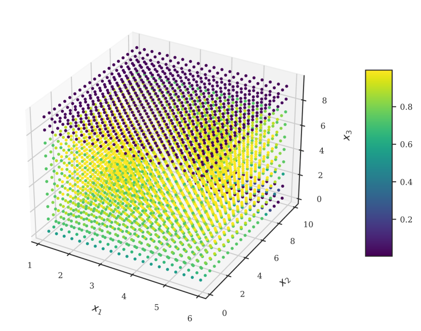
Figure 11: Maximum lower bound probabilities in the anesthesia delivery problem (for a grid of initial state) to remain in the safe set within the horizon of $20$ time steps.

Automated Anesthesia Delivery

We extend the automated anesthesia (propofol) delivery benchmark from Abate et al. (2018) with epistemic uncertainty in the pharmacokinetic system parameters. This benchmark models the concentration of propofol administered to a patient as a three-compartment pharmacokinetic model. The continuous-time, parametric version of this model is written as follows:

$$\dot{x}=\begin{bmatrix}-(k_{10}+k_{12}+k{13})&k_{12}&k_{13}\\ k_{21}&-k_{21}&0\\ k_{31}&0&-k_{31}\end{bmatrix}x+\begin{bmatrix}\frac{1}{V_{1}}\\ 0\\ 0\end{bmatrix}u,$$ (48)

where the state $x\in\amsmathbb{R}^{3}$ represents the propofol concentration in each of the three compartments, and where $u\in\amsmathbb{R}$ is the amount of propofol given to the patient. Parameters $V_{1}$, $k_{ij},i,j\in\{1,2,3\}$ are patient-specific parameters. We discretize Eq. 48 at a time step of $20\text{\,}\mathrm{s}$, assuming a zero-order hold (i.e., piece-wise constant) control input.

Capturing uncertainty.

We use the same parameter values as those reported by Abate et al. (2018) and assume that parameters $k_{10}$, $k_{21}$, and $V_{1}$ are uncertain within $\pm 10\%$ of their nominal values. To capture these uncertain parameters, we write Eq. 48 in the form of Eq. 1 with $r=2^{3}=8$ matrices $A_{1},\ldots,A_{r}$ and $B_{1},\ldots,B_{r}$. In addition to this epistemic uncertainty, we also add a stochastic process noise, which is assumed to have a zero-mean Gaussian distribution with a diagonal covariance matrix $10^{-3}I_{3}$, where $I_{3}\in\amsmathbb{R}^{n\times n}$ is the identity matrix.

Planning problem and abstraction.

We consider a safety problem, where the goal is to keep the propofol concentration within a safe set $\mathcal{Z}=[1,6]\times[0,10]\times[0,10]$ for $20$ discrete time steps. We partition the continuous state space into $20\times 20\times 20=8\,000$ discrete regions, yielding an iMDP with this same number of states. We apply Theorem 1 with $20$K noise samples, but with the approximate counting scheme described in Appendix B, we reduce the number of samples to around $1\,000$.

Results.

We present a 3-dimensional heatmap of the optimal reachability probabilities $\underline{Pr}^{\pi^{\star}}(\mathcal{M}{I}\models\varphi_{s_{I}}^{K})$ under the robust optimal iMDP policy for different initial states in Fig. 11. Recall from Theorem 2 that these results are lower bound guarantees on the performance of a controller in practice. We observe that, except when the initial concentration in compartment 3 is too high (approximately above 8), we are able to synthesize a controller that enables the system to remain in the safe set for the horizon of $20$ discrete steps. However, when the initial concentration in compartment 3 is too high, no safe controller could be synthesized, as reflected by the low probabilities shown in Fig. 11.

References

- Abate et al. (2018) Abate, A.; Blom, H. A. P.; Cauchi, N.; Haesaert, S.; Hartmanns, A.; Lesser, K.; Oishi, M.; Sivaramakrishnan, V.; Soudjani, S.; Vasile, C. I.; and Vinod, A. P. 2018. ARCH-COMP18 Category Report: Stochastic Modelling. In ARCH@ADHS, volume 54 of EPiC Series in Computing, 71–103. EasyChair.
- Abate et al. (2008) Abate, A.; Prandini, M.; Lygeros, J.; and Sastry, S. 2008. Probabilistic reachability and safety for controlled discrete time stochastic hybrid systems. Automatica, 44(11): 2724 – 2734.
- Alur et al. (2000) Alur, R.; Henzinger, T. A.; Lafferriere, G.; and Pappas, G. J. 2000. Discrete abstractions of hybrid systems. Proc. IEEE, 88(7): 971–984.
- Badings et al. (2022) Badings, T. S.; Abate, A.; Jansen, N.; Parker, D.; Poonawala, H. A.; and Stoelinga, M. 2022. Sampling-Based Robust Control of Autonomous Systems with Non-Gaussian Noise. In AAAI, 9669–9678. AAAI Press.
- Badings et al. (2021) Badings, T. S.; Jansen, N.; Poonawala, H. A.; and Stoelinga, M. 2021. Filter-Based Abstractions with Correctness Guarantees for Planning under Uncertainty. CoRR, abs/2103.02398.
- Baier and Katoen (2008) Baier, C.; and Katoen, J. 2008. Principles of model checking. MIT Press.
- Ben-Tal, Ghaoui, and Nemirovski (2009) Ben-Tal, A.; Ghaoui, L. E.; and Nemirovski, A. 2009. Robust Optimization, volume 28 of Princeton Series in Applied Mathematics. Princeton University Press.
- Berkenkamp et al. (2017) Berkenkamp, F.; Turchetta, M.; Schoellig, A. P.; and Krause, A. 2017. Safe Model-based Reinforcement Learning with Stability Guarantees. In NIPS, 908–918.
- Blanchini and Miani (2008) Blanchini, F.; and Miani, S. 2008. Set-theoretic methods in control, volume 78. Springer.
- Bobaru, Pasareanu, and Giannakopoulou (2008) Bobaru, M. G.; Pasareanu, C. S.; and Giannakopoulou, D. 2008. Automated Assume-Guarantee Reasoning by Abstraction Refinement. In CAV, volume 5123 of Lecture Notes in Computer Science, 135–148. Springer.
- Boucheron, Lugosi, and Massart (2013) Boucheron, S.; Lugosi, G.; and Massart, P. 2013. Concentration Inequalities - A Nonasymptotic Theory of Independence. Oxford University Press.
- Brunke et al. (2022) Brunke, L.; Greeff, M.; Hall, A. W.; Yuan, Z.; Zhou, S.; Panerati, J.; and Schoellig, A. P. 2022. Safe Learning in Robotics: From Learning-Based Control to Safe Reinforcement Learning. Annual Review of Control, Robotics, and Autonomous Systems, 5(1): 411–444.
- Campi, Carè, and Garatti (2021) Campi, M. C.; Carè, A.; and Garatti, S. 2021. The scenario approach: A tool at the service of data-driven decision making. Annu. Rev. Control., 52: 1–17.
- Campi and Garatti (2008) Campi, M. C.; and Garatti, S. 2008. The Exact Feasibility of Randomized Solutions of Uncertain Convex Programs. SIAM J. Optim., 19(3): 1211–1230.
- Campi and Garatti (2011) Campi, M. C.; and Garatti, S. 2011. A Sampling-and-Discarding Approach to Chance-Constrained Optimization: Feasibility and Optimality. J. Optim. Theory Appl., 148(2): 257–280.
- Casella and Berger (2021) Casella, G.; and Berger, R. L. 2021. Statistical inference. Cengage Learning.
- Cauchi and Abate (2019) Cauchi, N.; and Abate, A. 2019. StocHy: Automated Verification and Synthesis of Stochastic Processes. In TACAS (2), volume 11428 of Lecture Notes in Computer Science, 247–264. Springer.
- Cauchi et al. (2019) Cauchi, N.; Laurenti, L.; Lahijanian, M.; Abate, A.; Kwiatkowska, M.; and Cardelli, L. 2019. Efficiency through uncertainty: scalable formal synthesis for stochastic hybrid systems. In HSCC, 240–251. ACM.
- Charpentier et al. (2022) Charpentier, B.; Senanayake, R.; Kochenderfer, M. J.; and Günnemann, S. 2022. Disentangling Epistemic and Aleatoric Uncertainty in Reinforcement Learning. CoRR, abs/2206.01558.
- Chou, Ozay, and Berenson (2021) Chou, G.; Ozay, N.; and Berenson, D. 2021. Model Error Propagation via Learned Contraction Metrics for Safe Feedback Motion Planning of Unknown Systems. In CDC, 3576–3583. IEEE.
- Depeweg et al. (2018) Depeweg, S.; Hernández-Lobato, J. M.; Doshi-Velez, F.; and Udluft, S. 2018. Decomposition of Uncertainty in Bayesian Deep Learning for Efficient and Risk-sensitive Learning. In ICML, volume 80 of Proceedings of Machine Learning Research, 1192–1201. PMLR.
- Fan et al. (2022) Fan, C.; Qin, Z.; Mathur, U.; Ning, Q.; Mitra, S.; and Viswanathan, M. 2022. Controller Synthesis for Linear System With Reach-Avoid Specifications. IEEE Trans. Autom. Control., 67(4): 1713–1727.
- Fisac et al. (2015) Fisac, J. F.; Chen, M.; Tomlin, C. J.; and Sastry, S. S. 2015. Reach-avoid problems with time-varying dynamics, targets and constraints. In HSCC, 11–20. ACM.
- Fox and Ülkümen (2011) Fox, C. R.; and Ülkümen, G. 2011. Distinguishing two dimensions of uncertainty. In Perspectives on Thinking, Judging, and Decision Making. Universitetsforlaget.
- García and Fernández (2015) García, J.; and Fernández, F. 2015. A comprehensive survey on safe reinforcement learning. J. Mach. Learn. Res., 16: 1437–1480.
- Geibel and Wysotzki (2005) Geibel, P.; and Wysotzki, F. 2005. Risk-Sensitive Reinforcement Learning Applied to Control under Constraints. J. Artif. Intell. Res., 24: 81–108.
- Geromel and Colaneri (2006) Geromel, J. C.; and Colaneri, P. 2006. Robust stability of time varying polytopic systems. Systems & Control Letters, 55(1): 81–85.
- Givan, Leach, and Dean (2000) Givan, R.; Leach, S. M.; and Dean, T. L. 2000. Bounded-parameter Markov decision processes. Artif. Intell., 122(1-2): 71–109.
- Haesaert, den Hof, and Abate (2017) Haesaert, S.; den Hof, P. M. J. V.; and Abate, A. 2017. Data-driven and model-based verification via Bayesian identification and reachability analysis. Autom., 79: 115–126.
- Haesaert et al. (2018) Haesaert, S.; Nilsson, P.; Vasile, C. I.; Thakker, R.; Agha-mohammadi, A.; Ames, A. D.; and Murray, R. M. 2018. Temporal Logic Control of POMDPs via Label-based Stochastic Simulation Relations. In ADHS, volume 51 of IFAC-PapersOnLine, 271–276. Elsevier.
- Hüllermeier and Waegeman (2021) Hüllermeier, E.; and Waegeman, W. 2021. Aleatoric and epistemic uncertainty in machine learning: an introduction to concepts and methods. Mach. Learn., 110(3): 457–506.
- Jackson et al. (2020) Jackson, J.; Laurenti, L.; Frew, E. W.; and Lahijanian, M. 2020. Safety Verification of Unknown Dynamical Systems via Gaussian Process Regression. In CDC, 860–866. IEEE.
- Kenanian et al. (2019) Kenanian, J.; Balkan, A.; Jungers, R. M.; and Tabuada, P. 2019. Data driven stability analysis of black-box switched linear systems. Autom., 109.
- Knuth et al. (2021) Knuth, C.; Chou, G.; Ozay, N.; and Berenson, D. 2021. Planning With Learned Dynamics: Probabilistic Guarantees on Safety and Reachability via Lipschitz Constants. IEEE Robotics Autom. Lett., 6(3): 5129–5136.
- Kumar and Varaiya (2015) Kumar, P. R.; and Varaiya, P. 2015. Stochastic systems: Estimation, identification, and adaptive control. SIAM.
- Kwiatkowska, Norman, and Parker (2011) Kwiatkowska, M. Z.; Norman, G.; and Parker, D. 2011. PRISM 4.0: Verification of Probabilistic Real-Time Systems. In CAV, volume 6806 of Lecture Notes in Computer Science, 585–591. Springer.
- Lahijanian, Andersson, and Belta (2015) Lahijanian, M.; Andersson, S. B.; and Belta, C. 2015. Formal Verification and Synthesis for Discrete-Time Stochastic Systems. IEEE Trans. Autom. Control., 60(8): 2031–2045.
- Lavaei et al. (2022) Lavaei, A.; Soudjani, S.; Abate, A.; and Zamani, M. 2022. Automated verification and synthesis of stochastic hybrid systems: A survey. Automatica, 146: 110617.
- Lavaei et al. (2023) Lavaei, A.; Soudjani, S.; Frazzoli, E.; and Zamani, M. 2023. Constructing MDP Abstractions Using Data With Formal Guarantees. IEEE Control. Syst. Lett., 7: 460–465.
- Loquercio, Segù, and Scaramuzza (2020) Loquercio, A.; Segù, M.; and Scaramuzza, D. 2020. A General Framework for Uncertainty Estimation in Deep Learning. IEEE Robotics Autom. Lett., 5(2): 3153–3160.
- Majumdar and Tedrake (2017) Majumdar, A.; and Tedrake, R. 2017. Funnel libraries for real-time robust feedback motion planning. Int. J. Robotics Res., 36(8): 947–982.
- Makdesi, Girard, and Fribourg (2021) Makdesi, A.; Girard, A.; and Fribourg, L. 2021. Data-Driven Abstraction of Monotone Systems. In L4DC, volume 144 of Proceedings of Machine Learning Research, 803–814. PMLR.
- Modares (2022) Modares, H. 2022. Data-driven Safe Control of Linear Systems Under Epistemic and Aleatory Uncertainties. CoRR, abs/2202.04495.
- Pereira et al. (2020) Pereira, M.; Wang, Z.; Exarchos, I.; and Theodorou, E. A. 2020. Safe Optimal Control Using Stochastic Barrier Functions and Deep Forward-Backward SDEs. In CoRL, volume 155 of Proceedings of Machine Learning Research, 1783–1801. PMLR.
- Peruffo and Mazo (2023) Peruffo, A.; and Mazo, M. 2023. Data-Driven Abstractions With Probabilistic Guarantees for Linear PETC Systems. IEEE Control. Syst. Lett., 7: 115–120.
- Puggelli et al. (2013) Puggelli, A.; Li, W.; Sangiovanni-Vincentelli, A. L.; and Seshia, S. A. 2013. Polynomial-Time Verification of PCTL Properties of MDPs with Convex Uncertainties. In CAV, volume 8044 of Lecture Notes in Computer Science, 527–542. Springer.
- Romao, Margellos, and Papachristodoulou (2020) Romao, L.; Margellos, K.; and Papachristodoulou, A. 2020. Tight generalization guarantees for the sampling and discarding approach to scenario optimization. In CDC, 2228–2233. IEEE.
- Romao, Papachristodoulou, and Margellos (2022) Romao, L.; Papachristodoulou, A.; and Margellos, K. 2022. On the exact feasibility of convex scenario programs with discarded constraints. IEEE Transactions on Automatic Control (to appear).
- Salamati and Zamani (2022) Salamati, A.; and Zamani, M. 2022. Safety Verification of Stochastic Systems: A Repetitive Scenario Approach. IEEE Control Systems Letters.
- Shmarov and Zuliani (2015) Shmarov, F.; and Zuliani, P. 2015. ProbReach: verified probabilistic delta-reachability for stochastic hybrid systems. In HSCC, 134–139. ACM.
- Smith (2013) Smith, R. C. 2013. Uncertainty quantification: theory, implementation, and applications, volume 12. Siam.
- Sullivan (2015) Sullivan, T. J. 2015. Introduction to uncertainty quantification, volume 63. Springer.
- Thiebes, Lins, and Sunyaev (2021) Thiebes, S.; Lins, S.; and Sunyaev, A. 2021. Trustworthy artificial intelligence. Electron. Mark., 31(2): 447–464.
- Thrun, Burgard, and Fox (2005) Thrun, S.; Burgard, W.; and Fox, D. 2005. Probabilistic robotics. Intelligent robotics and autonomous agents. MIT Press.
- Tsiamis and Pappas (2019) Tsiamis, A.; and Pappas, G. J. 2019. Finite Sample Analysis of Stochastic System Identification. In CDC, 3648–3654. IEEE.
- Vinod, Gleason, and Oishi (2019) Vinod, A. P.; Gleason, J. D.; and Oishi, M. M. K. 2019. SReachTools: a MATLAB stochastic reachability toolbox. In HSCC, 33–38. ACM.
- Vinod, Israel, and Topcu (2022) Vinod, A. P.; Israel, A.; and Topcu, U. 2022. On-the-Fly Control of Unknown Nonlinear Systems With Sublinear Regret. IEEE Transactions on Automatic Control, 1–13.
- Wiesemann, Kuhn, and Sim (2014) Wiesemann, W.; Kuhn, D.; and Sim, M. 2014. Distributionally Robust Convex Optimization. Oper. Res., 62(6): 1358–1376.
- Wolff, Topcu, and Murray (2012) Wolff, E. M.; Topcu, U.; and Murray, R. M. 2012. Robust control of uncertain Markov Decision Processes with temporal logic specifications. In CDC, 3372–3379. IEEE.
- Yedavalli (2014) Yedavalli, R. K. 2014. Robust control of uncertain dynamic systems. AMC, 10: 12.
- Zanon and Gros (2021) Zanon, M.; and Gros, S. 2021. Safe Reinforcement Learning Using Robust MPC. IEEE Trans. Autom. Control., 66(8): 3638–3652.
- Zikelic et al. (2022) Zikelic, D.; Lechner, M.; Henzinger, T. A.; and Chatterjee, K. 2022. Learning Control Policies for Stochastic Systems with Reach-avoid Guarantees. CoRR, abs/2210.05308.