CLEEGN: A Convolutional Neural Network for Plug-and-Play Automatic EEG Reconstruction

Abstract

Human electroencephalography (EEG) is a brain monitoring modality that senses cortical neuroelectrophysiological activity in high-temporal resolution. One of the greatest challenges posed in applications of EEG is the unstable signal quality susceptible to inevitable artifacts during recordings. To date, most existing techniques for EEG artifact removal and reconstruction are applicable to offline analysis solely, or require individualized training data to facilitate online reconstruction. We have proposed CLEEGN, a novel convolutional neural network for plug-and-play automatic EEG reconstruction. CLEEGN is based on a subject-independent pre-trained model using existing data and can operate on a new user without any further calibration. The performance of CLEEGN was validated using multiple evaluations including waveform observation, reconstruction error assessment, and decoding accuracy on well-studied labeled datasets. The results of simulated online validation suggest that, even without any calibration, CLEEGN can largely preserve inherent brain activity and outperforms leading online/offline artifact removal methods in the decoding accuracy of reconstructed EEG data. In addition, visualization of model parameters and latent features exhibit the model behavior and reveal explainable insights related to existing knowledge of neuroscience. We foresee pervasive applications of CLEEGN in prospective works of online plug-and-play EEG decoding and analysis.

1 Introduction

Since the first record of human electroencephalogram (EEG) performed almost a century ago (in 1924), EEG has been one of the most widely used non-invasive neural modalities that monitors brain activity in high temporal resolution (Koike et al., 2013; Mehta & Parasuraman, 2013; Sejnowski et al., 2014). Among a variety of modalities, EEG has extensive use in the clinical assessment of neurological and psychiatric conditions, as well as in the research of neuroscience, cognitive science, psychology, and brain-computer interfacing (BCI).

EEG signals measure subtle fluctuations of the electrical field driven by local neuroelectrophysiological activity of a population of neurons in the brain cortex (Cohen, 2017). While the electrodes are placed on the surface of the scalp, undesired artifacts may introduce interruption in the measurements and distort the signal of interest. Even in a well-controlled laboratory with a well-trained subject who can maximally keep the body still and relaxed, the EEG signals, unfortunately, could be contaminated by inevitable behavioral and physiological artifacts such as eye blinks, reflective muscle movements, ocular activity, cardiac activity, etc (Croft & Barry, 2000; Wallstrom et al., 2004; Romero et al., 2008). In practice, it is difficult to identify and track the sources of artifacts entirely due to their diversity and non-stationarity. Noise cancellation and artifact removal remain major issues in EEG signal processing and decoding.

Currently, numerous methods have been proposed to alleviate the influence of artifacts in EEG signals. Traditional EEG denoising algorithms include filtering, regression, data separation or decomposition (Makeig et al., 1995; Islam et al., 2016; Kothe & Jung, 2016). According to previous meta-analyses on EEG artifact removal literature (Urigüen & Garcia-Zapirain, 2015; Jiang et al., 2019), independent component analysis (ICA) is especially popular. It is majorly used in $45\%$ of EEG denoising literature. ICA-based artifact removal estimates the component activity by unmixing the EEG data in the channel domain. Through manual or automatic identification, one can exclude the artifact components and then reconstruct the EEG data through back projection based on non-artifact components (Jung et al., 2000a). The fast growth of deep learning methods has drawn state-of-the-art performances in a variety of machine learning problems (LeCun et al., 2015). Lately, deep-learning-based EEG reconstruction has drawn much attention (Leite et al., 2018; Sun et al., 2020; Lopes et al., 2021; Lee et al., 2020; Chuang et al., 2022). Although these methods can effectively remove artifacts from artificial synthetic signals, their performance in reconstructing real EEG data has not yet been validated in terms of decoding labeled EEG data. Meanwhile, the model design of existing deep-learning-based techniques for EEG reconstruction rarely takes the characteristics of EEG into account.

In this work, we propose CLEEGN, a ConvoLutional neural network for EEG reconstructioN. CLEEGN is capable of subject-independent EEG construction without any training/calibration for a new subject. The contributions of this work are three-fold:

• a light-weight autoencoder CNN, CLEEGN, with a subject-independent framework that facilitates plug-and-play EEG reconstruction.

• CLEEGN outperforms leading online/offline methods in providing reconstructed EEG data with the best decoding performance for BCI datasets.

• with a novel model design dedicated to EEG reconstruction, CLEEGN characterizes patterns of EEG interpretable and provides neuroscientific insights.

2 Related Work

Current processing techniques for EEG artifact removal are highly varied based on the context where the algorithm may apply. Earlier attempts of EEG denoising assumed that the EEG signals and artifacts appear in different frequency ranges. Based on the assumption, some significant artifacts can be eliminated by the linear filtering method during the online stage (Seifzadeh et al., 2014). Despite the advantages of low computational time, linear filtering hardly removes artifacts that distribute in an overlapped frequency range of EEG signals. Another approach, adaptive filtering (Schlögl et al., 2007), estimates artifact signals through additional EOG, EMG, ECG channels and removes these noisy signals from the recording signals by regression. Nevertheless, this approach requires additional auxiliary electrodes and raises the cost and inconvenience in practical applications. The blind source separation (BSS) method in EEG denoising was developed by assuming that the recording EEG signals are linear combinations of the signals from noise sources and the brain neurons. One of the most well-known BSS method is independent component analysis (ICA) (Jung et al., 2000a; b), which is able to separate EEG signals into independent components (ICs) (Makeig et al., 1995).

Traditionally, the artifact components extracted by ICA are determined and removed through manual inspection. Recently developed ICLabel can label the ICs provenance into seven different categories: brain, eye, heart, muscle, line noise, channel noise, and other (Pion-Tonachini et al., 2019). Artifact subspace reconstruction (ASR) is another automatic approach, which is based on the principal component analysis (PCA) method (Kothe & Jung, 2016). The ASR method selects relatively noiseless periods from the multi-channel EEG data as reference based on the data distribution. After projecting all EEG data to the principal-component domain, high-variance components projected from the artifacts are detected by a cutoff parameter $k$. The noiseless signals are reconstructed by preserving the components without carrying artifacts and back-projected to the time domain. The ASR method has been shown capable of improving the quality of ICA decomposition (Chang et al., 2020).

Recently, neural network-based methods have been proposed to remove artifacts for EEG data. A variety of network structures have been applied to the framework for removing EEG artifacts and reconstructing clean EEG. A deep convolutional autoencoder (Leite et al., 2018) can enhance the peak-signal-to-noise ratio compared to the linear filtering method via a common CNN autoencoder structure, which has been widely used on image denoising. Their work shows that it seems practicable to transform the EEG waveform through a CNN structure. Later on, a combined framework integrating Bayesian deep learning and ICA (Lee et al., 2020) used thresholding of the EEG data distribution to discard ICs classified as ocular artifacts. These methods leverage the flexibility of deep learning model design and achieve improvements in their assessments. Considering the non-stationary property in EEG data and the degradation phenomenon during training, 1D-ResCNN (Sun et al., 2020) was proposed, which adopted an Inception-Residual module in the network structure. This network is able to remove EOG, ECG, EMG on single-channel synthesis EEG data. Instead of using synthesis EEG data, IC-U-Net (Chuang et al., 2022) was created, which generated pairings of noisy and noiseless EEG data through ICA as training data. The proposed neural network is a one-dimensional adaptation of U-Net architecture trained with the ensemble of four loss functions to minimize the difference between amplitude, velocity, acceleration, and frequency components from the signals. This work showed that their reconstructed signal has higher SNR and can surely increase the number of brain components classified by ICLabel.

3 Materials and Methods

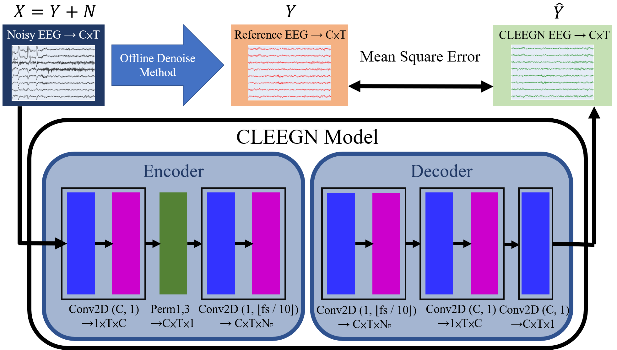
Figure 1: Illustration of the proposed CLEEGN model architecture and the model training flow.

CLEEGN Architecture and Model Training. CLEEGN is designed to map multi-channel noisy EEG into a latent space and reconstruct it into noiseless EEG signals. The architecture of CLEEGN is shown in Figure 1. The architecture of the encoder is inspired by an existing CNN model designed for EEG recognition (Wei et al., 2019) and incorporates convolutional blocks that capture spatiotemporal characteristics of EEG data. The first convolution block is used to extract spatial EEG features through a convolutional layer containing $C$ spatial filters whose shape is $(C,1)$, where $C$ is the number of electrodes of the EEG signals. The second convolution block is used to extract temporal EEG features through a convolutional layer containing $N_{F}$ temporal filters with shape $(1,\lfloor f_{s}\times 0.1\rfloor)$, where $f_{s}$ denotes the sample frequency of the EEG signals. As for the decoder, we design an approximately symmetric structure to the encoder with three convolutional blocks. The first convolutional block decodes the EEG feature with $N_{F}$ temporal kernels with shape is $(1,\lfloor f_{s}\times 0.1\rfloor)$. The second block decodes the EEG feature by a convolution layer with $C$ spatial kernels of shape $(C,1)$. The last convolutional block is for projecting the feature domain back to the original time domain. To maintain the shape between the model inputs and outputs, every convolution block applies zero-padding except the first block in the encoder. The detail of the CLEEGN architecture is available in Table 1.

Table 1: The architecture of CLEEGN.

Block	Layer	#kernels	Size	Output shape
Encoder	Input			($B$, $C$, $T$, 1)
	Conv2D	$C$	($C$, 1)	($B$, 1, $T$, $C$)
	Permute			($B$, $C$, $T$, 1)
	BatchNorm
	Conv2D	$N_{F}$	(1, $\lfloor f_{s}/10\rfloor$)	($B$, $C$, $T$, $N_{F}$)
	BatchNorm
Decoder	Conv2D	$N_{F}$	(1, $\lfloor f_{s}/10\rfloor$)	($B$, $C$, $T$, $N_{F}$)
	BatchNorm
	Conv2D	$C$	($C$, 1)	($B$, $C$, $T$, $C$)
	BatchNorm
	Conv2D	1	($C$, 1)	($B$, $C$, $T$, 1)
$C$: # channels, $T$: # time points, $f_{s}$: Sampling rate, $B$: Batch size

As illustrated in Figure 1, the objective of the proposed method is to minimize the difference between noiseless signals, $Y$, and the model output, $\hat{Y}$. The recording EEG data, $X$, is the combination of brain signals, $Y$, and the signals from multiple noise sources, $N$. CLEEGN is a denoising autoencoder that is intended to perform artifact removal on EEG data by creating a mapping between multi-channel noisy EEG signals, $X$, and noiseless signals, $Y$. The training process of CLEEGN utilizes pairing noisy raw EEG data and noiseless reference EEG data so that the model can learn to transform noisy EEG data into reconstructed EEG data with maximal similarity to the reference data. To generate large-scale reference EEG data, we adopted automatic denoising methods, ICLabel and ASR, to remove artifacts and reconstruct clean waveforms offline. The pairing EEG recording with $C$ channels of continuous noisy/noiseless data was further segmented into training sample pairs. The input size is ($C$, $T$), where $T$ is the number of time points based on the sampling rate of the EEG data in $4$-second segments. The windows size and stride are set as $T$ and $0.5T$. In the context of plug-and-play EEG reconstruction, CLEEGN was trained as a subject-independent model. To perform subject-independent training and testing, we grouped subjects into $k$ disjoint sets. During the training process, one of the sets was left out for testing. Subjects’ EEG data in the left-alone set were not involved in both training and validation. A complete experiment on a single dataset would result in $k$ different models. The artifact removal performance of a model was evaluated by using the left-alone set. The number of subjects in one set and the EEG duration available for each subject depend on the experiment setting and the dataset used.

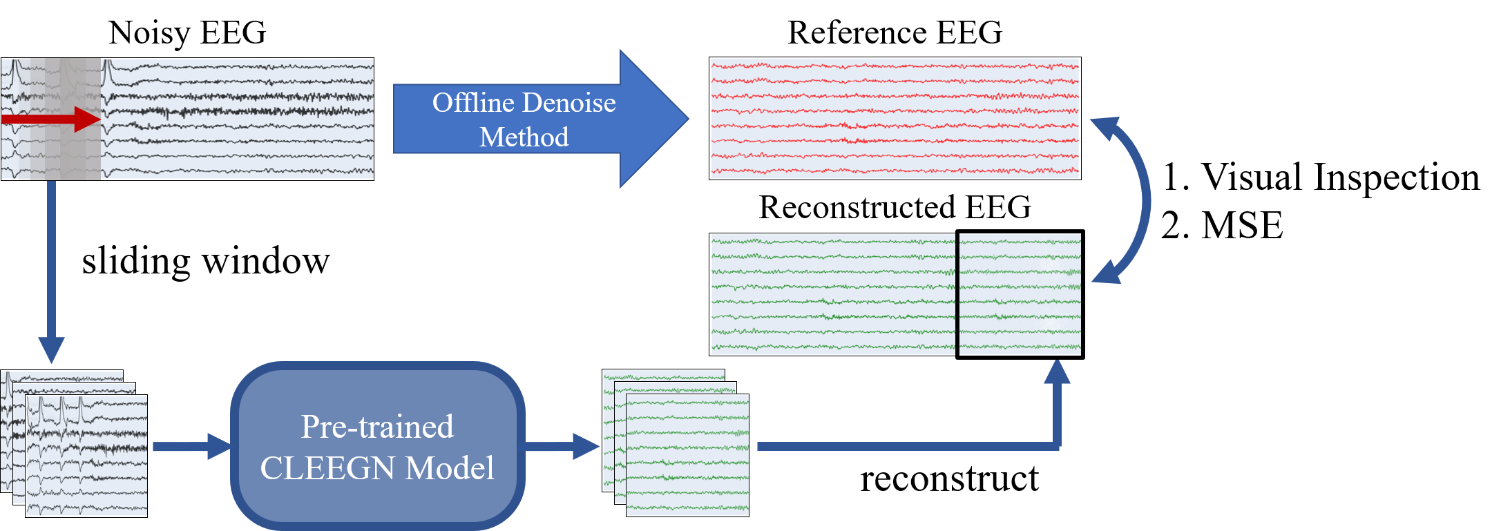
Figure 2: Schematic of the simulated online processing flow and the assessments of fitness between the reconstructed and reference EEG signals.

EEG Reconstruction and Evaluation. The reconstructed EEG data of CLEEGN is generated through an online reconstruction simulation. In the online stage, the system performs artifact removal on a new subject using a pre-trained CLEEGN model without any requirement of training/calibration. Figure 2 shows the online EEG reconstruction simulated in offline. The EEG data from a subject in the left-alone set would be fed into the model sequentially. The stride size of the sliding window is set to $0.5$ seconds to minimize the delay in online reconstruction. The fitness of the model can be evaluated by observing the waveform visually or measuring the similarity using the mean square error (MSE) between reconstructed and noiseless EEG. Meanwhile, we propose to use the decoding performance of labeled EEG data as an objective measurement of the reconstructed EEG quality. We employed EEGNet, a compact CNN for end-to-end EEG decoding (Lawhern et al., 2018), as the classifier to decode the labeled EEG data in our study.

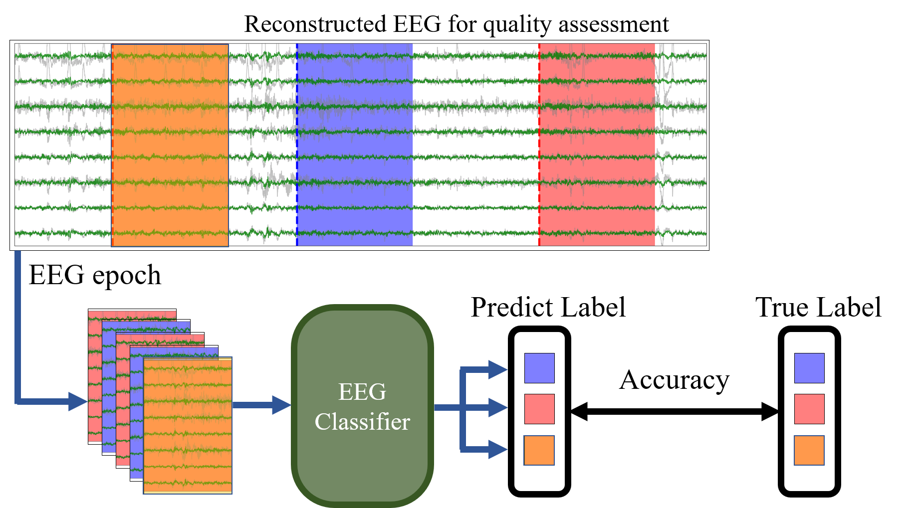
Figure 3: Objective EEG quality assessment of the reconstructed EEG based on the decoding performance.

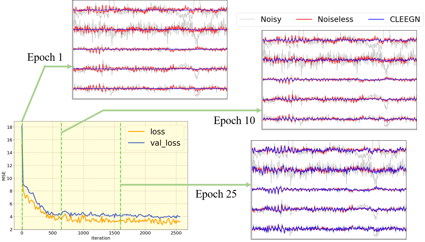
Figure 4: Reconstructed EEG signals by CLEEGN across training steps.

4 Experiments

Data and Model Fitting. In this work, we applied two labeled EEG datasets, the BCI-ERN dataset and the MAMEM-SSVEP-II dataset . We estimate the classification performance by calculating the score of Area Under the Curve (AUC) in ERN binary classification and Top-1 accuracy in the SSVEP task. Figure 3 is the schematic diagram of the process of decoding performance estimation using the reconstructed EEG data. The segmented EEG epochs are divided into three splits within each subject: training set, validation set, and test set. The ratio between classes remained the same in each set. We perform 20 repeated runs with shuffled data to estimate the average performance of each decoding performance evaluation. Detailed descriptions of the two datasets are available in the appendix at A.2. Figure 4 presents the loss curve and the reconstruction result at the end of three different training iterations in a sample run using the ERN dataset. Through this exploration, we can look into the course of model fitting. In the early stage of training, the model reduces the large MSE loss by smoothing the input signals. To further minimize the error between reconstruction and reference (offline denoised signal), the model compensates the intensity to better fit the reference signals. At the convergent stage of training, we can see the reconstructed waveform is very similar to the one in reference data.

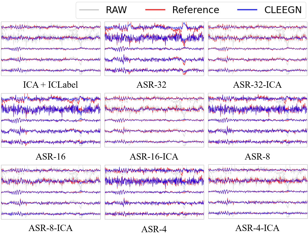
Figure 5: Visualization of raw (gray), reference (red), CLEEGN (blue) EEG waveforms with offline methods by ICLabel, ASR-32, ASR-32-ICLabel, ASR-16, ASR-16-ICLabel, ASR-8, ASR-8-ICLabel, ASR-4, ASR-4-ICLabel. Each segment plots a five-second segment of signals at Fp1, T7, Cz, T8, and O2.

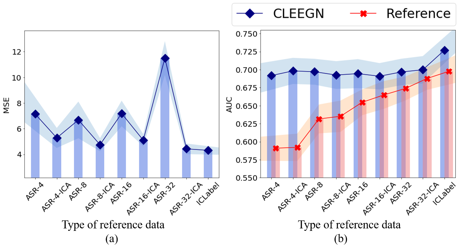
Figure 6: (a) Overall fitness of the CLEEGN model across types of reference data using the ERN dataset. (b) Decoding performance of the CLEEGN-reconstructed EEG data (blue) and the corresponding reference data used for CLEEGN model training (red).

Types of Reference Data. As ICLabel, ASR, and the hybrid ASR-ICLabel are employed to automatically generate large-scale noiseless reference EEG data offline, it is of our interest to investigate what type of reference EEG serves as the best noiseless reference data for the CLEEGN model training. Figure 5 presents the EEG waveforms sampled from Subject 2 in the ERN dataset. The EEG time series from top to bottom represent the recording of Fp1, T7, Cz, T8, and O2 channels. The nine sub-figures visualize the comparison between the noisy raw data and the reference data reconstructed by the ICLabel, ASR with or without ICLabel when the cutoff parameter $k$ was set to 4, 8, 16, and 32. We can see the waveform of ICLabel and the ASR-ICLabel hybrid method with 4 different cutoff parameters $k$ are similar, and the noiseless waveform reconstructed by CLEEGN are highly correlated to the result from these 5 methods. High-amplitude ocular artifacts such as blinking and eye saccades are phenomenal in frontal channels (Fp1) and muscular artifacts featuring high-frequency (around 24-30 Hz in the $\beta$ band) are observed on the T7 channel. CLEEGN, ICA, and ASR-ICLabel hybrid methods can eliminate these kinds of artifacts. Compared to the ICLabel and ASR-ICLabel hybrid methods, ASR is unable to eliminate the high-frequency EMG artifact for this dataset. The tolerance of large amplitude EOG artifact increases with the employment of larger cutoff parameter $k$. Limited by the reference data generated by ASR, CLEEGN preserves the high-frequency artifact. As for the large amplitude artifacts that failed to be identified by ASR-32 and ASR-16, we can see that CLEEGN is able to mitigate those EOG artifacts. As shown in Figure 6(a), the reference data prepared by ICLabel offer the lowest MSE, i.e. the best fitness for CLEEGN training. We also compare the types of reference EEG data and their corresponding CLEEGN reconstruction results in the decoding performance of the ERN EEG dataset to assess their data quality. As illustrated in Figure 6(b), CLEEGN reconstruction draws better performances for all denoising methods. Although the performance decreases with a smaller cutoff parameter $k$, CLEEGN can outperform the reference data used for its training. This result suggests that our method not only removes the artifact but also preserves informative brain activity in the EEG under our cross-subject training scheme. As the ICLabel provides the reference data with the best decoding performance and fitness, we chose ICLabel as the source of reference data for further experiments in this study.

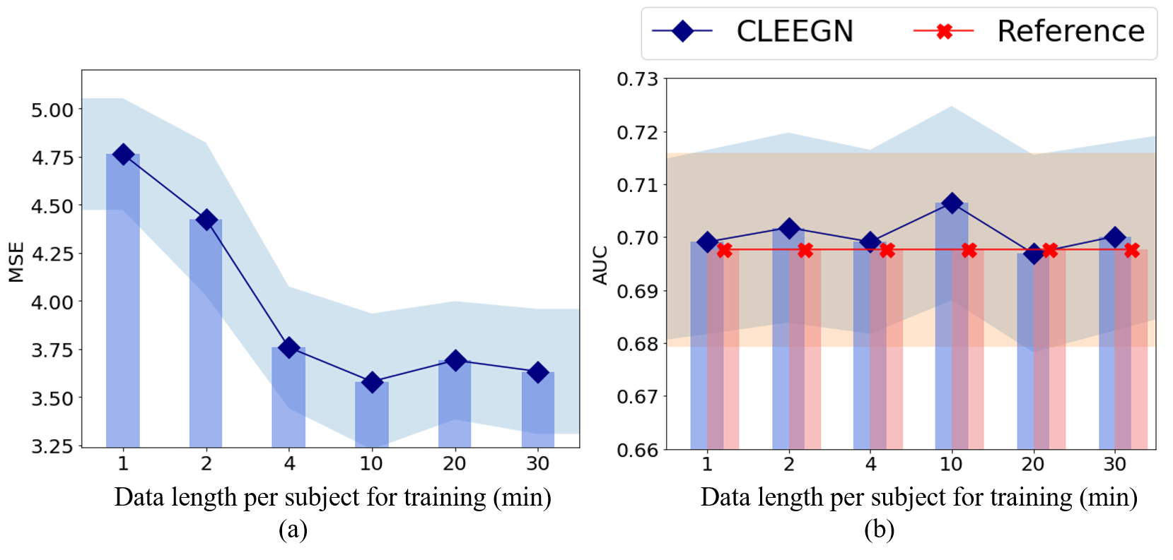
Figure 7: Performance of CLEEGN against the training data length per subject evaluated by the BCI-ERN dataset on (a) the fitness to the reference data; and (b) the decoding performance.

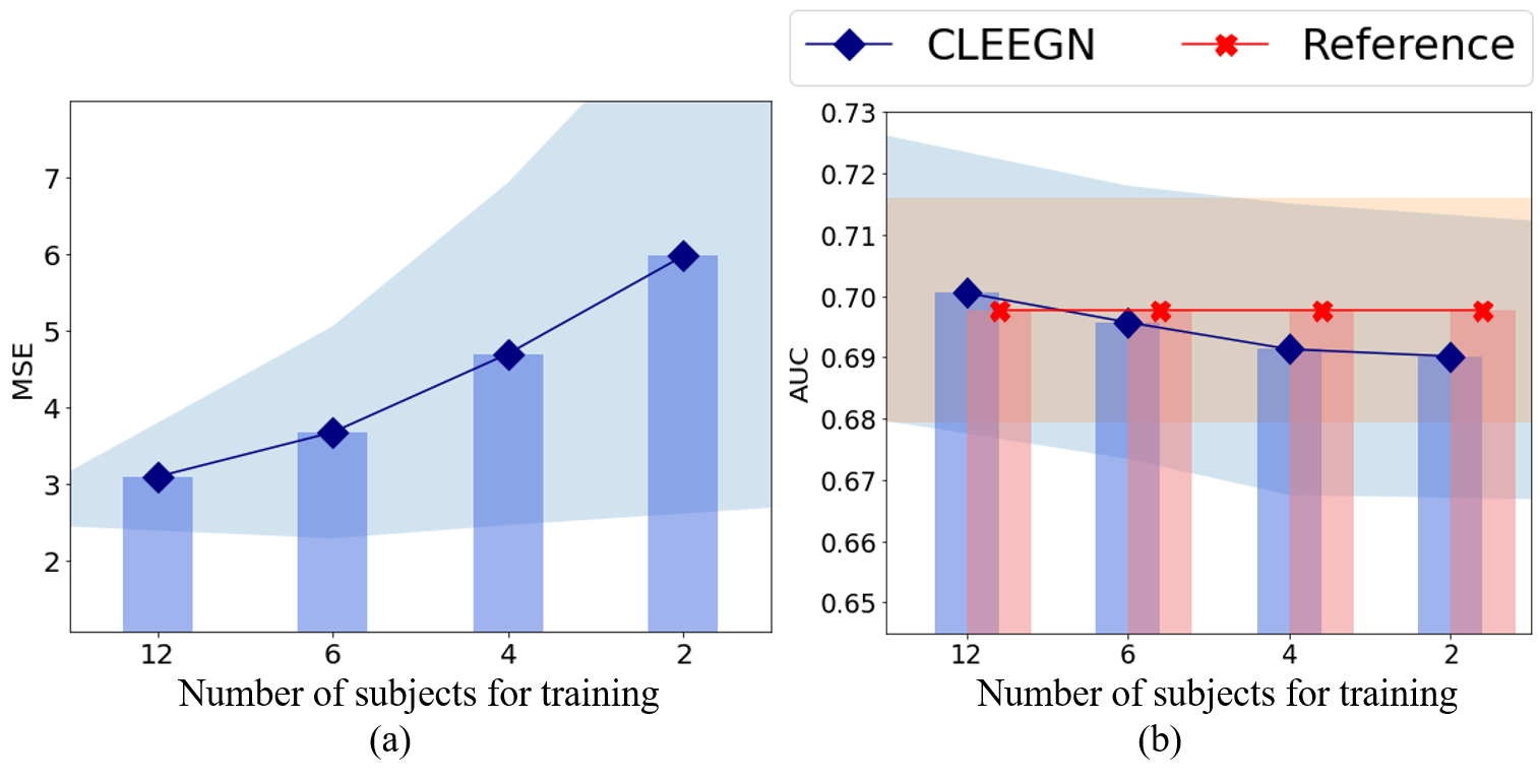
Figure 8: EEG reconstruction performance of CLEEGN against the number of subjects evaluated under the BCI-ERN dataset by (a) the fitness to the reference data; and (b) the decoding performance.

Table 2: Overall performance over all subjects in the BCI-ERN dataset.

Method	MSE $\downarrow$	AUC $\uparrow$	Total parameters $\downarrow$
ICLabel	–	0.7218$\pm$0.0197	–
1D-ResCNN	6.7147$\pm$0.5025	0.6697$\pm$0.0175	325891
IC-U-Net	5.2086$\pm$0.4204	0.6949$\pm$0.0140	2683192
CLEEGN	3.5984$\pm$0.2538	0.7252$\pm$0.0189	220755

Table 3: Overall performance over all subjects in the MAMEM-SSVEP-II dataset.

Method	MSE $\downarrow$	Accuracy $\uparrow$	Total parameters $\downarrow$
ICLabel	–	0.4940$\pm$0.0667	–
1D-ResCNN	0.2047$\pm$0.0524	0.2908$\pm$0.0316	313735
IC-U-Net	0.0698$\pm$0.0085	0.3422$\pm$0.0253	2664724
CLEEGN	0.0777$\pm$0.0111	0.5159$\pm$0.0622	14043

Training Data Size. We explored the effect of data length per subject in the training set regarding the fitness and the decoding performance of CLEEGN. The training data were segmented from the first 1, 2, 4, 10, 20, and 30 minutes of data in each EEG recording to investigate the trade-off between training time and reconstruction performance. Figure 7(a) shows the fitness of CLEEGN to the reference data. The model trained using the first 10 minutes obtain the minimal value among all duration configurations. Though the difference in MSE between 10, 20, and 30 minutes is not noticeable, Figure 7(b) shows that using the 10-minute training data yields the best decoding performance among all settings. Interestingly, with only one-minute training data from each subject, CLEEGN can achieve comparable decoding performance to the reference data. This indicates that CLEEGN retains its performance even when each subject only contributes a short recording for training. In addition, we explore the effect of the number of subjects included in the training set on the fitness of CLEEGN model training and the decoding performance of the reconstructed EEG data. We randomly reduced the number of subjects for training from 12 to 6, 4, and 2. Since the subset of subjects may influence the performance, we tested multiple combinations and averaged the results. With the decrease in the number of subjects, the MSE value and the standard error (light span area) increase in Figure 8(a), which indicates that the generalization ability of the CLEEGN model reduces when fewer subjects are included for training. In Figure 8(b), we can observe a slight decrease in decoding performance. We consider the number of subjects as an essential factor in the performance of CLEEGN, yet it requires only a few subjects to achieve a satisfactory performance compared to the reference data.

Performance Comparison. We compare the performance of CLEEGN against three baseline methods, ICLabel, 1D-ResCNN, and IC-U-Net. Except for the ICLabel that operates offline, CLEEGN and the other two neural network-based methods perform a simulated online reconstruction based on the same training process with the reference data generated by ICLabel. Results of the ERN EEG dataset are shown in Table 2. CLEEGN has the best fitness to the reference data with the minimum MSE, the highest AUC score in the decoding performance, and the least parameters. For the SSVEP EEG data, although not having the minimum MSE, CLEEGN outperforms other methods in the decoding accuracy and the model size. The evaluation across the two datasets suggests an overall superiority of our proposed CLEEGN model over other existing neural network-based methods in online reconstruction. CLEEGN even provides a better reconstruction than the offline ICLabel. These promising results indicate the usability of CLEEGN in online training/calibration-free EEG reconstruction that truly meets the need for real-world applications of EEG-based BCI.

Visualization. On account of the interpretability of the CLEEGN model, we visualized its intermediate latent features by mapping onto a 2-dimensional domain based on the principal component analysis (PCA) of the noisy raw EEG data (Wold et al., 1987). Figure 9(a) shows the principal component space and the noisy EEG data channel projections. We observe that the scatters of noisy EEG data retain the spatial relationship of the actual EEG electrodes. The arrangement of frontal electrodes (prefix in Fp, P) to the posterior (prefix in P, O) are projected along the x-axis from right to left. The projection from top to bottom matches the left-side electrodes (suffixed in odd numbers), central electrode (suffixed in z), and right-side electrodes (suffixed in even numbers). The projection suggests that EEG data of adjacent channels tend to show similar waveforms. The blue dots in Figure 9(b), (c) are the projection of latent features resulting from the first and second convolutional layers, which make up the encoder design of CLEEGN. The projection of latent features from the next two convolutional layers is presented in Figure 9(d), (e). From Figure 9(b) to (e), we can see the distribution range of the latent features shrink in the encoder design and expand in the decoder design of CLEEGN. Figure 9(f) compares the distribution of noisy data and CLEEGN reconstructed data, showing that the CLEEGN reconstructed data is a more compact cluster than the noisy EEG in the PCA space. This implies that the process within CLEEGN includes a projection of the original EEG data in the upstream layer, complex temporal filtering and combination in the midstream layers, and a final projection that converts the noiseless latent features back to the channel domain.

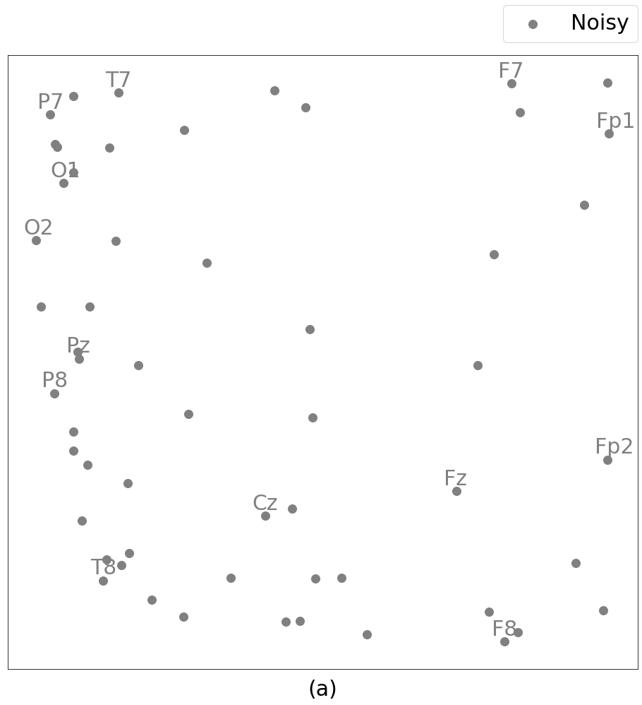
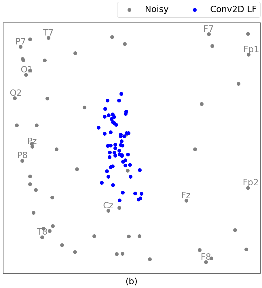
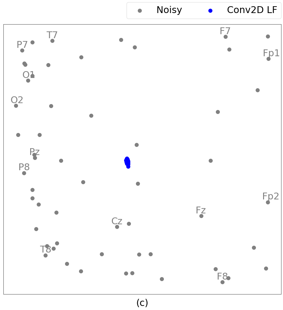
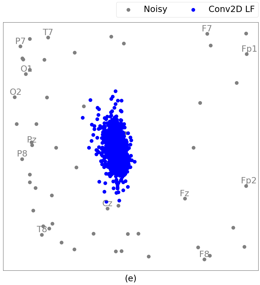
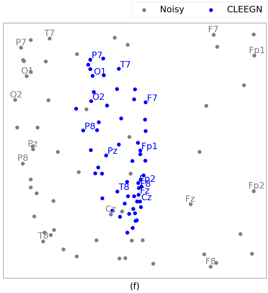
Figure 9: PCA visualization of latent features in CLEEGN for a single subject in the ERN dataset. (a) The noisy EEG data projected on the PCA space of the noisy EEG data. (b)-(e) Latent features in the first to fourth convolutional layers projected on the original noisy PCA space. (f) CLEEGN reconstructed EEG data projected on the original noisy PCA space.

5 Conclusion

In this work, we have proposed CLEEGN, a novel convolutional neural network for plug-and-play automatic EEG reconstruction. The training of CLEEGN leverages the conventional offline denoising methods, ASR and ICLabel, with automatic component classification to generate abundant noiseless EEG data. The performance of CLEEGN was objectively validated using multiple evaluations including waveform observation; reconstruction error assessment; and decoding accuracy on well-studied, labeled datasets. The experiment results suggest that, even without any calibration, CLEEGN can predominantly preserve inherent brain activity. According to the decoding performance of reconstructed EEG data, CLEEGN outperforms other neural network-based denoising methods on both ERN and SSVEP EEG decoding. From the visualization of the waveform, CLEEGN can remove artifacts from different sources and the waveform is highly correlated to the reference data. Through the visualization of model parameters and latent features, we exhibit model behavior and reveal explainable insights related to existing knowledge of neuroscience. We foresee pervasive applications of CLEEGN in prospective works of EEG decoding and analysis.

6 Acknowledgement

This work was supported in part by the National Science and Technology Council (109-2222-E-009-006-MY3, 110-2221-E-A49-130-MY2, and 110-2314-B-037-061) and in part by the Higher Education Sprout Project of the National Yang Ming Chiao Tung University and Ministry of Education of Taiwan.

Appendix A Appendix

A.1 Neural Network Training Configuration

A.1.1 CLEEGN

For training CLEEGN, we used the Adam optimizer with an initial learning rate of 1e-3 without weight decay. Besides, the exponential learning rate scheduler is applied with a gamma of 0.8. As for the loss function, we used Mean Squared Error (MSE). The batch size is set to 64 and the total training epoch is 40. During the training procedure, the model is evaluated using the validation subset at the end of every epoch with the purpose of saving the weights that achieved the lowest validation loss.

A.1.2 IC-U-Net

The optimizer adopted in IC-U-Net (Chuang et al., 2022) training is SGD with an initial learning rate of 1e-2, momentum of 0.9, and weight decay of 5e-4. The learning rate scheduler used in the training procedure is the multistep scheduler. As for the loss function, a novel ensemble loss proposed in IC-U-Net is adopted. This ensemble is a simple linear combination of the Mean Squared Error (MSE) in amplitude, velocity, acceleration, and frequency components of EEG signals. Each term in the loss function has same weight. The batch size is set to 64 and the total training epoch is 200. The weight saving strategy in IC-U-Net training is the same as CLEEGN.

A.1.3 1D-ResCNN

The Adam optimizer with an initial learning rate of 1e-3 and the Mean Squared Error (MSE) loss function is adopted in 1D-ResCNN (Sun et al., 2020) training. Since the 1D-ResCNN is developed under one-dimensional synthesized EEG data and no explicit instruction of using multi-channel EEG provided, we trained 1D-ResCNN using two different method. For one method, we trained multiple models for each EEG channel respectively. For the other method, we viewed each multi-channel EEG segment as a batch and the channel arrangement within a batch is fixed. Under our experiment, the result showed that the second method not only provides an efficient training process, but also results in a better reconstructed performance. The same weight saving strategy in CLEEGN is adopted in 1D-ResCNN training.

A.1.4 Decoding Performance Evaluation Model: EEGNet

EEGNet (Lawhern et al., 2018) is a famous EEG decoding model and widely used in EEG literature. In the original EEGNet paper, they investigated their proposed model with a different number of kernels and denoted the model with $F_{1}$ temporal filters and $D$ spatial filters as EEGNet-$F_{1}$,$D$. We use two different settings to train the two datasets used. In ERN classification, we use the EEGNet-8,2 structure suggested by the EEGNet paper. As for the SSVEP classification, an experimental result showed that EEGNet-100,8 can draw the best performance. We trained and evaluated the decoding performance individually for each subject. We divided the collection of event epochs into three splits within each subject: training set, validation set, and test set with a ratio of 3:1:1. The ratio between classes remained the same in each set. The loss function is categorical cross entropy (CCE) and the Adam optimizer is adopted with a learning rate of $10^{-3}$ and zero weight decay. The batch size is set to 32 and the total training epoch is 200.

A.2 Description of Datasets

A.2.1 Dataset 1: Feedback Error-Related Negativity (ERN)

Error-related negativity (ERN) can be categorized as a kind of event-related potential (ERP), which occurs after an erroneous or abnormal event perceived by the subject. One characteristic of the feedback ERN is a relatively large negative amplitude approximately 350 ms and a positive amplitude approximately 500 ms after visual feedback triggered by the error event. In this work, we mainly use a well-studied EEG dataset from the BCI Challenge competition hosted by Kaggle to evaluate the artifact removal effectiveness. This dataset includes EEG recordings of 26 subjects (16 subjects labeled and 10 subjects unlabeled) that participated in a P300 speller task. P300 speller is a well-known BCI system that develops a typing application through P300 response evoked potential. The ERN experiment was conducted under the assumption that the ERN occurred if the subject received incorrect prediction (feedback) from the P300 speller. The objective of the competition was to improve the P300 speller performance by implementing error correction through ERN potentials. We used the 16 subjects with labeled data of which the sampling rate is 200 Hz initially with 56 passive Ag/AgCl EEG sensors.

In the interest of increasing the usability of EEG data, we applied some pre-processing procedures to each EEG recording. The EEG data were down-sampled to 128 Hz and re-referenced by the common average reference (CAR) method to eliminate common-mode noise and to zero-center the data. Each recording was band-pass filtered to 1-40 Hz through the FIR filter implemented by EEGLAB to remove DC drifting. During EEG decoding evaluation, we epoch EEG signals in [0, 1.25] second interval to obtain correct and erroneous feedback.

A.2.2 Dataset 2: Steady state visually evoked potential (SSVEP)

Steady state visually evoked potential (SSVEP) is another kind of ERP that is characterized as periodic potential induced by rapidly repetitive visual stimulation. The SSVEP is composed of several discrete frequency components, which consist of the fundamental frequency of the visual stimulus as well as its harmonics. To investigate the generalization ability of the model, we use ”EEG SSVEP Dataset II” from Multimedia Authoring & Management using your Eyes & Mind (MAMEM). The dataset includes EEG data from 11 subjects and consists of five different frequencies (6.66, 7.50, 8.57, 10.00, and 12.00 Hz). Each subject was recorded in five sessions and each session included 25 trials (5 trials for each class). The data used a 256-channel HydroCel Geodesic Sensor Net (HCGSN) and captured the signals with a sampling rate of 250 Hz. Since there are several different bad channels in each subject’s EEG recording, we preserved 20 common channels from each subject to train the CLEEGN model. Every recording was down-sampled to 125 Hz, re-referenced by the common average reference (CAR) method, and band-pass filtered to 1-40 Hz. We epoch EEG signals in [1, 5] second interval for each event recorded timestamp. The first second was discarded under the consideration of a reaction delay of the subject.

A.3 Investigation of Decoding Performance Evaluation: SSVEP

In this work, we mainly use decoding performance as the assessment of different artifact removal methods. We provide an interpretation of the relationship between EEG quality and decoding performance. In Section 4 SSVEP result, IC-U-Net can optimize the weight with minimal MSE value among all compared artifact removal networks. However, the decoding performance is worse than CLEEGN and even the reference method (ICLabel), which implies that the average error over data points (MSE) is not the best assessment of EEG quality.

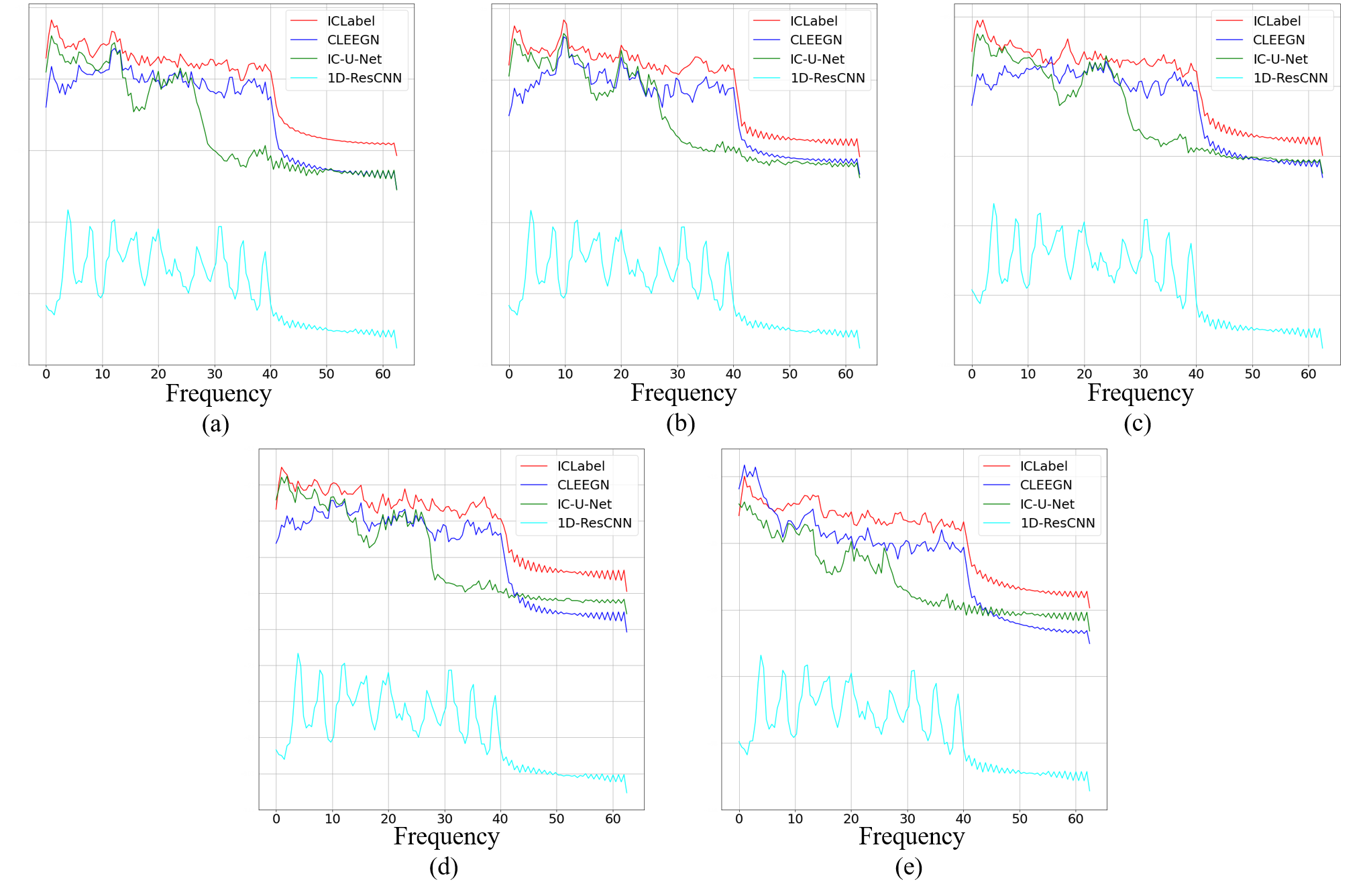
Figure 10: Power spectrum density of EEG data on different methods to each class

In the SSVEP experiment, the fundamental frequency of the external rapidly repetitive visual stimulation and its harmonics can be an important feature in classification. Hence, higher quality in the frequency component of EEG data is required. We use the power spectrum density (PSD) to interpret the result of decoding performance. Figure 10 shows the PSD of EEG event data in each class denoised by different methods. We can see the reconstructed EEG spectrum from CLEEGN in each class is similar to the reference. As for IC-U-Net, it seems that the model can not completely reconstruct in several frequency bands (15-20Hz, 30-40Hz), which leads to the low decoding performance. The PSD result shows that there is great distortion in the power density of reconstructed data generated by 1D-ResCNN. Since 1D-ResCNN is a one-dimensional structure, we hypothesize that spatial information is important in EEG artifact removal.

A.4 Additional tables

Method	ICLabel		ASR-32		ASR-32-ICA
Subject	MSE	AUC	MSE	AUC	MSE	AUC
S02	3.2835	0.8432	9.4341	0.8102	3.6285	0.8398
S06	2.5723	0.6609	10.7221	0.6234	2.7348	0.6093
S07	4.7804	0.7835	17.2428	0.7155	4.6049	0.6889
S11	7.2317	0.6214	9.2276	0.5939	6.7069	0.6243
S12	3.2090	0.7126	16.5107	0.6789	3.0982	0.6794
S13	4.3666	0.7860	9.7730	0.7937	4.0034	0.7849
S14	2.0056	0.8256	2.6510	0.7951	1.9174	0.8030
S16	6.3664	0.6758	15.2617	0.6437	5.9677	0.6542
S17	4.5280	0.8068	10.1852	0.8080	8.1861	0.8023
S18	4.3724	0.7629	9.2606	0.6835	3.6407	0.7331
S20	4.6405	0.7022	11.5464	0.6898	3.7116	0.6669
S21	5.0383	0.7219	21.3344	0.6827	5.0986	0.6569
S22	4.5625	0.7300	20.2808	0.6334	4.8429	0.6850
S23	3.4311	0.7086	3.8892	0.6991	2.5044	0.7163
S24	3.2064	0.7310	4.7346	0.7297	3.6940	0.7045
S26	5.3556	0.5614	11.9691	0.5661	6.4727	0.5475

Table 4: Mean square error between reference denoising method and CLEEGN (MSE), AUC score of CLEEGN (AUC) in ”BCI-Challenge” ERN dataset - Part1

Method	ASR-16		ASR-16-ICA		ASR-8
Subject	MSE	AUC	MSE	AUC	MSE	AUC
S02	4.2217	0.8205	3.5384	0.8425	4.0614	0.8205
S06	4.4036	0.5513	3.2639	0.6388	3.9688	0.6388
S07	11.4515	0.7116	5.1372	0.6588	8.2052	0.6717
S11	8.4986	0.5803	4.9902	0.6061	7.0836	0.5983
S12	7.1270	0.6980	4.1351	0.6690	4.6099	0.7005
S13	5.0222	0.7870	6.5591	0.7680	4.5217	0.7778
S14	2.2373	0.8137	2.5573	0.7723	2.6699	0.7982
S16	9.6206	0.6680	4.9104	0.6554	6.8716	0.6660
S17	18.8896	0.8076	10.9239	0.8041	27.6019	0.8141
S18	5.2366	0.7139	3.6065	0.7264	4.3582	0.7006
S20	6.7533	0.6843	5.5760	0.6668	4.3853	0.6776
S21	8.5629	0.6501	6.6647	0.6338	6.4900	0.6674
S22	9.3490	0.6395	5.1241	0.6460	6.7729	0.6419
S23	3.1867	0.6795	4.4331	0.6874	2.4365	0.7022
S24	2.7711	0.7191	3.7558	0.7130	3.7320	0.7117
S26	7.6073	0.5861	6.4456	0.5648	9.1152	0.5652

Table 5: Mean square error between reference denoising method and CLEEGN (MSE), AUC score of CLEEGN (AUC) in ”BCI-Challenge” ERN dataset - Part2

Method	ASR-8-ICA		ASR-4		ASR-4-ICA
Subject	MSE	AUC	MSE	AUC	MSE	AUC
S02	3.4726	0.8277	4.0551	0.8204	3.3401	0.8249
S06	2.9740	0.6257	4.4043	0.5893	4.1949	0.6526
S07	5.4224	0.6423	8.4744	0.6592	4.7362	0.6969
S11	4.3832	0.6035	9.2528	0.5868	4.9227	0.5972
S12	3.5382	0.6800	3.9801	0.6969	3.8259	0.6732
S13	5.4227	0.7921	5.5527	0.7833	6.5429	0.7628
S14	2.1820	0.8004	3.6646	0.7947	2.9259	0.8057
S16	4.8361	0.6685	8.4332	0.6379	4.0452	0.6757
S17	11.1061	0.8014	24.9330	0.8102	16.4403	0.8141
S18	3.4891	0.7191	4.0793	0.7468	3.2979	0.7322
S20	4.6687	0.6625	4.9512	0.6444	4.6338	0.6505
S21	6.1690	0.6518	5.0372	0.6479	4.5595	0.6507
S22	5.1410	0.6399	6.7985	0.6566	5.5497	0.6801
S23	3.5369	0.6935	3.6311	0.6993	3.9354	0.6870
S24	2.8299	0.7215	4.2418	0.7231	3.7892	0.7075
S26	6.8030	0.5495	12.7965	0.5704	7.7062	0.5595

Table 6: Mean square error between reference denoising method and CLEEGN (MSE), AUC score of CLEEGN (AUC) in ”BCI-Challenge” ERN dataset - Part3

DataLength (min)	ICLabel	30		20		10
Subject	AUC	MSE	AUC	MSE	AUC	MSE	AUC
S02	0.8114	3.4818	0.8290	3.6152	0.8359	3.5139	0.8191
S06	0.6281	2.4449	0.6117	2.4496	0.6195	2.3353	0.6215
S07	0.7298	4.1740	0.7177	4.3742	0.6744	4.2118	0.7166
S11	0.5971	7.0916	0.6050	6.8226	0.6107	7.6580	0.6037
S12	0.6916	2.6238	0.6700	2.7464	0.6724	2.3652	0.6949
S13	0.7859	3.7257	0.7855	3.9133	0.7774	3.5441	0.7926
S14	0.7888	1.7715	0.7766	1.7445	0.7959	1.6376	0.8086
S16	0.6503	5.5278	0.6585	5.5853	0.6811	5.2618	0.6878
S17	0.8198	4.6574	0.8162	4.4208	0.8069	4.4521	0.8066
S18	0.6997	3.3821	0.6965	3.4677	0.6899	3.7442	0.7045
S20	0.6829	3.4097	0.6873	3.8692	0.6669	3.4116	0.6960
S21	0.6198	4.0377	0.6760	3.7572	0.6918	3.7251	0.6733
S22	0.6372	3.2582	0.6920	3.4192	0.6383	3.0667	0.6600
S23	0.6985	2.3770	0.6994	2.6990	0.7050	2.3144	0.7213
S24	0.7339	2.1982	0.7108	2.1782	0.7317	2.0520	0.7396
S26	0.5867	3.9663	0.5701	3.9898	0.5524	4.0011	0.5566

Table 7: Mean square error between reference denoising method and CLEEGN (MSE), AUC score of CLEEGN (AUC) in ”BCI-Challenge” ERN dataset trained by different data length - Part1

DataLength (min)	ICLabel	4		2		1
Subject	AUC	MSE	AUC	MSE	AUC	MSE	AUC
S02	0.8114	3.2609	0.8101	3.1745	0.8324	3.3467	0.8213
S06	0.6281	2.2442	0.6093	3.0822	0.6135	3.3718	0.6302
S07	0.7298	4.2698	0.6655	4.6784	0.6774	3.8478	0.7180
S11	0.5971	6.5970	0.6135	7.6816	0.6406	4.5129	0.6193
S12	0.6916	2.7294	0.6948	2.7830	0.6733	3.7798	0.6717
S13	0.7859	3.4267	0.7793	5.7493	0.8007	6.3488	0.7760
S14	0.7888	1.6493	0.7934	2.2690	0.7937	2.5422	0.7980
S16	0.6503	5.9354	0.6681	7.9410	0.6594	5.2486	0.6584
S17	0.8198	4.5170	0.7939	4.7344	0.7965	5.8205	0.7986
S18	0.6997	3.8781	0.7546	4.6024	0.7202	4.7593	0.7239
S20	0.6829	4.1724	0.6721	4.3053	0.6837	5.9014	0.6707
S21	0.6198	4.5480	0.6905	4.8047	0.6494	5.2452	0.6497
S22	0.6372	3.3430	0.6629	4.0498	0.6772	5.7725	0.6739
S23	0.6985	2.9178	0.6939	3.1362	0.6936	4.3290	0.6796
S24	0.7339	2.3747	0.7173	2.8420	0.7468	4.5555	0.7275
S26	0.5867	4.2618	0.5666	4.9736	0.5705	6.8117	0.5682

Table 8: Mean square error between reference denoising method and CLEEGN (MSE), AUC score of CLEEGN (AUC) in ”BCI-Challenge” ERN dataset trained by different data length - Part2

Method	ICLabel		CLEEGN		IC-U-Net		1D-ResCNN
Subject	MSE	AUC	MSE	AUC	MSE	AUC	MSE	AUC
S02	-	0.8238	3.5139	0.8274	4.4294	0.7816	5.7621	0.7598
S06	-	0.6616	2.3353	0.6926	4.1464	0.6132	5.4486	0.5601
S07	-	0.8263	4.2118	0.7410	4.3550	0.7003	6.5909	0.6848
S11	-	0.6083	7.6580	0.6324	5.0279	0.6153	5.1880	0.5729
S12	-	0.6947	2.3652	0.6756	3.8519	0.6587	7.0038	0.6283
S13	-	0.7913	3.5441	0.7835	8.1448	0.7469	8.1590	0.7509
S14	-	0.8128	1.6376	0.8135	2.9057	0.7674	3.7053	0.7679
S16	-	0.6402	5.2618	0.6615	4.0351	0.6405	6.1420	0.6485
S17	-	0.8177	4.4521	0.8153	8.2195	0.7612	7.8305	0.7564
S18	-	0.7419	3.7442	0.7667	4.7798	0.7082	6.4393	0.6729
S20	-	0.6962	3.4116	0.6770	5.7497	0.6802	8.9663	0.6359
S21	-	0.7130	3.7251	0.7742	5.1049	0.7132	7.4864	0.6718
S22	-	0.7166	3.0667	0.7435	6.1630	0.7199	10.6583	0.6749
S23	-	0.7016	2.3144	0.7316	4.3579	0.6848	3.6919	0.6524
S24	-	0.7366	2.0520	0.7228	3.7706	0.7186	4.7246	0.7245
S26	-	0.5663	4.0011	0.5445	8.2955	0.6077	9.6387	0.5539

Table 9: ERN mean square error and AUC score of each subject on different network structure

Method	ICLabel		CLEEGN		IC-U-Net		1D-ResCNN
Subject	MSE	Top-1 Acc	MSE	Top-1 Acc	MSE	Top-1 Acc	MSE	Top-1 Acc
S001	-	0.6930	0.0859	0.6620	0.0852	0.4570	0.1228	0.2335
S002	-	0.7350	0.1379	0.8000	0.0609	0.3235	0.0608	0.2315
S003	-	0.3175	0.1113	0.3645	0.1013	0.2830	0.1798	0.2325
S004	-	0.2610	0.1040	0.2770	0.0984	0.2380	0.1896	0.2330
S005	-	0.2870	0.0387	0.2985	0.0475	0.2685	0.0539	0.2310
S006	-	0.5300	0.0237	0.5595	0.0322	0.3910	0.0583	0.2290
S007	-	0.5110	0.0819	0.4935	0.0768	0.4035	0.1503	0.2340
S008	-	0.2020	0.1143	0.2270	0.1169	0.2015	0.1205	0.2345
S009	-	0.9050	0.0492	0.8005	0.0460	0.4070	0.3755	0.4070
S010	-	0.5560	0.0405	0.5055	0.0379	0.3690	0.3125	0.5260
S011	-	0.4360	0.0668	0.6870	0.0651	0.4225	0.6281	0.4075

Table 10: SSVEP mean square error and top-1 accuracy of each subject on different network structure

References

- Chang et al. (2020) Chi-Yuan Chang, Sheng-Hsiou Hsu, Luca Pion-Tonachini, and Tzyy-Ping Jung. Evaluation of artifact subspace reconstruction for automatic artifact components removal in multi-channel eeg recordings. IEEE Transactions on Biomedical Engineering, 67(4):1114–1121, 2020. doi: 10.1109/TBME.2019.2930186.
- Chuang et al. (2022) Chun-Hsiang Chuang, Kong-Yi Chang, Chih-Sheng Huang, and Tzyy-Ping Jung. Ic-u-net: A u-net-based denoising autoencoder using mixtures of independent components for automatic eeg artifact removal. NeuroImage, 263:119586, 2022. ISSN 1053-8119.
- Cohen (2017) Michael X Cohen. Where does eeg come from and what does it mean? Trends in neurosciences, 40(4):208–218, 2017.
- Croft & Barry (2000) Rodney J Croft and Robert J Barry. Removal of ocular artifact from the eeg: a review. Neurophysiologie Clinique/Clinical Neurophysiology, 30(1):5–19, 2000.
- Islam et al. (2016) Md Kafiul Islam, Amir Rastegarnia, and Zhi Yang. Methods for artifact detection and removal from scalp eeg: A review. Neurophysiologie Clinique/Clinical Neurophysiology, 46(4):287–305, 2016. ISSN 0987-7053. doi: https://doi.org/10.1016/j.neucli.2016.07.002.
- Jiang et al. (2019) Xiao Jiang, Gui-Bin Bian, and Zean Tian. Removal of artifacts from eeg signals: a review. Sensors, 19(5):987, 2019.
- Jung et al. (2000a) Tzyy-Ping Jung, Scott Makeig, Colin Humphries, Te-Won Lee, Martin J Mckeown, Vicente Iragui, and Terrence J Sejnowski. Removing electroencephalographic artifacts by blind source separation. Psychophysiology, 37(2):163–178, 2000a.
- Jung et al. (2000b) Tzyy-Ping Jung, Scott Makeig, Marissa Westerfield, Jeanne Townsend, Eric Courchesne, and Terrence J Sejnowski. Removal of eye activity artifacts from visual event-related potentials in normal and clinical subjects. Clinical Neurophysiology, 111(10):1745–1758, 2000b.
- Koike et al. (2013) Shinsuke Koike, Yukika Nishimura, Ryu Takizawa, Noriaki Yahata, and Kiyoto Kasai. Near-infrared spectroscopy in schizophrenia: a possible biomarker for predicting clinical outcome and treatment response. Frontiers in psychiatry, 4:145, 2013.
- Kothe & Jung (2016) Christian Andreas Edgar Kothe and Tzyy-Ping Jung. Artifact removal techniques with signal reconstruction, 2016. US Patent 14/895,440.
- Lawhern et al. (2018) Vernon J Lawhern, Amelia J Solon, Nicholas R Waytowich, Stephen M Gordon, Chou P Hung, and Brent J Lance. Eegnet: a compact convolutional neural network for eeg-based brain–computer interfaces. Journal of neural engineering, 15(5):056013, 2018.
- LeCun et al. (2015) Yann LeCun, Yoshua Bengio, and Geoffrey Hinton. Deep learning. nature, 521(7553):436–444, 2015.
- Lee et al. (2020) Sangmin S Lee, Kiwon Lee, and Guiyeom Kang. Eeg artifact removal by bayesian deep learning & ica. In 2020 42nd Annual International Conference of the IEEE Engineering in Medicine & Biology Society (EMBC), pp. 932–935. IEEE, 2020.
- Leite et al. (2018) Niago Moreira Nobre Leite, Eanes Torres Pereira, Edmar Candeia Gurjão, and Luciana Ribeiro Veloso. Deep convolutional autoencoder for eeg noise filtering. In 2018 IEEE International Conference on Bioinformatics and Biomedicine (BIBM), pp. 2605–2612. IEEE, 2018.
- Lopes et al. (2021) Fábio Lopes, Adriana Leal, Júlio Medeiros, Mauro F. Pinto, António Dourado, Matthias Dümpelmann, and César Teixeira. Automatic electroencephalogram artifact removal using deep convolutional neural networks. IEEE Access, 9:149955–149970, 2021.
- Makeig et al. (1995) Scott Makeig, Anthony Bell, Tzyy-Ping Jung, and Terrence J Sejnowski. Independent component analysis of electroencephalographic data. In D. Touretzky, M.C. Mozer, and M. Hasselmo (eds.), Advances in Neural Information Processing Systems, volume 8. MIT Press, 1995.
- Mehta & Parasuraman (2013) Ranjana K Mehta and Raja Parasuraman. Neuroergonomics: a review of applications to physical and cognitive work. Frontiers in human neuroscience, 7:889, 2013.
- Pion-Tonachini et al. (2019) Luca Pion-Tonachini, Ken Kreutz-Delgado, and Scott Makeig. Iclabel: An automated electroencephalographic independent component classifier, dataset, and website. NeuroImage, 198:181–197, 2019.
- Romero et al. (2008) Sergio Romero, Miguel A Mañanas, and Manel J Barbanoj. A comparative study of automatic techniques for ocular artifact reduction in spontaneous eeg signals based on clinical target variables: a simulation case. Computers in biology and medicine, 38(3):348–360, 2008.
- Schlögl et al. (2007) A. Schlögl, C. Keinrath, D. Zimmermann, R. Scherer, R. Leeb, and G. Pfurtscheller. A fully automated correction method of eog artifacts in eeg recordings. Clinical Neurophysiology, 118(1):98–104, 2007. ISSN 1388-2457.
- Seifzadeh et al. (2014) Sahar Seifzadeh, Karim Faez, and Mahmood Amiri. Comparison of different linear filter design methods for handling ocular artifacts in brain computer interface system. Journal of Computer & Robotics, 7:51–56, 2014. ISSN 2345-6582.
- Sejnowski et al. (2014) Terrence J Sejnowski, Patricia S Churchland, and J Anthony Movshon. Putting big data to good use in neuroscience. Nature neuroscience, 17(11):1440, 2014.
- Sun et al. (2020) Weitong Sun, Yuping Su, Xia Wu, and Xiaojun Wu. A novel end-to-end 1d-rescnn model to remove artifact from eeg signals. Neurocomputing, 404:108–121, 2020. ISSN 0925-2312.
- Urigüen & Garcia-Zapirain (2015) Jose Antonio Urigüen and Begoña Garcia-Zapirain. Eeg artifact removal—state-of-the-art and guidelines. Journal of neural engineering, 12(3):031001, 2015.
- Wallstrom et al. (2004) Garrick L Wallstrom, Robert E Kass, Anita Miller, Jeffrey F Cohn, and Nathan A Fox. Automatic correction of ocular artifacts in the eeg: a comparison of regression-based and component-based methods. International journal of psychophysiology, 53(2):105–119, 2004.
- Wei et al. (2019) Chun-Shu Wei, Toshiaki Koike-Akino, and Ye Wang. Spatial component-wise convolutional network (sccnet) for motor-imagery eeg classification. In 2019 9th International IEEE/EMBS Conference on Neural Engineering (NER), pp. 328–331. IEEE, 2019.
- Wold et al. (1987) Svante Wold, Kim Esbensen, and Paul Geladi. Principal component analysis. Chemometrics and intelligent laboratory systems, 2(1-3):37–52, 1987.