Travel the Same Path: A Novel TSP Solving Strategy

Abstract

In this paper, we provide a novel strategy for solving Traveling Salesman Problem, which is a famous combinatorial optimization problem studied intensely in the TCS community. In particular, we consider the imitation learning framework, which helps a deterministic algorithm making good choices whenever it needs to, resulting in a speed up while maintaining the exactness of the solution without suffering from the unpredictability and a potential large deviation.

Furthermore, we demonstrate a strong generalization ability of a graph neural network trained under the imitation learning framework. Specifically, the model is capable of solving a large instance of TSP faster than the baseline while has only seen small TSP instances when training.

Keywords:

Traveling salesman problem, Graph Neural Network, Imitation Training, Reinforcement Learning, Integer Programming, Embedding learning, Combinatorial Optimization, Exact solver.

1 Introduction

The traveling salesman problem (TSP) can be described as follows: given a list of cities and the distances between each pair of cities, find the shortest route possible that visits each city exactly once then returns to the origin city. Specifically, given an undirected weighted graph $\mathcal{G}=(\mathcal{E},\mathcal{V})$, with an ordered pair of nodes set $\mathcal{E}$ and an edge set $\mathcal{V}\subseteq\mathcal{E}\times\mathcal{E}$ where $\mathcal{G}$ is equipped with spatial structure. This means that each edge between nodes will have different weights and each node will have its coordinates, we want to find a simple cycle that visits every node exactly once while having the smallest cost.

We will utilize GCNN (Graph Convolutional Neural Network), a particular kind of GNN, together with imitation learning to solve TSP in an interesting and inspiring way. In particular, we focus on the generalization ability of models trained on small-sized problem instances.

2 Related Works

There has already been extensive work done to optimize TSP solvers both theoretically and practically. We have done extensive research into other solvers; the papers most relevant to our project are summarized below.

Transformer Network for TSP [6].

The main focus of this paper is to detail the application of deep reinforcement learning reapplied to a Transformer architecture originally created for Natural Language Processing (NLP). Unlike our proposed model, this solver does not solve TSP exactly but instead learns heuristics that have very low error rates (0.004% for TSP50 and 0.39% for TSP100). These heuristics can run over a TSP problem much faster than a traditional solver while still achieving similar results.

Exact Combinatorial Optimization with GCNNs [11].

This paper serves as one of the backbones of our research; its main focus is to detail how MIPS can potentially be solved much quicker than a traditional solver by using GNNs (specifically GCNNs). It did this by training its model using imitation learning (using the strong branching expert rule) and was able to effectively produce outputs for problem instances much greater than what they were trained on.

State of the Art Exact Solver.

There has been a lot of progress on the symmetric TSP in the last century. With the increase in the number of nodes, there is a super-polynomial (at least exponential) explosion in the number of potential solutions. This makes the TSP problem difficult to solve on two parameters, the first being finding a global shortest route as well as reducing the computation complexity in finding this route. Concorde [9], written in the ANSI C programming language is widely recognized as the fastest state-of-the-art (SOTA) exact TSP solution for large instances.

3 Preliminary

3.1 Integer Linear Programming Formulation of TSP

We first formulate TSP in terms of Integer Linear Programming. Given an undirected weighted group $\mathcal{G}=(\mathcal{E},\mathcal{V})$, we label the nodes with numbers $1,\ldots,n$ and define

$$x_{ij}\coloneqq\begin{dcases}1,&\text{if }(i,j)\in\mathcal{E}^{\prime}\\ 0,&\text{if }(i,j)\in\mathcal{E}\setminus\mathcal{E}^{\prime},\end{dcases}$$

where $\mathcal{E}^{\prime}\subset\mathcal{E}$ is a variable which can be viewed as a compact representation of all variables $x_{ij}$, $\forall i,j$. Furthermore, we denote the weight on edge $(i,j)$ by $c_{ij}$, then for a particular TSP problem instance, we can formulate the problem as follows.

$$\min \sum_{i=1}^{n}\sum_{j\neq i,j=1}^{n}c_{ij}x_{ij}$$ (1)

$$\sum_{i=1,i\neq j}^{n}x_{ij}=1 j=1,\ldots,n;$$

$$\sum_{j=1,j\neq i}^{n}x_{ij}=1 i=1,\ldots,n;$$

$$u_{i}-u_{j}+nx_{ij}\leq n-1 2\leq i\neq j\leq n;$$

$$1\leq u_{i}\leq n-1 2\leq i\leq n;$$

$$x_{ij}\in\{0,1\} i,j=1,\ldots,n;$$

$$u_{i}\in\mathbb{Z} i=2,\ldots,n.$$

This is the Miller-Tucker-Zemlin formulation [20]. Note that in our case, since we are solving TSP exactly, all variables are integers. This type of integer linear programming is sometimes known as pure integer programming.

3.2 Solving the Integer Linear Program

Since integer programming is an NP-Hard problem, there is no known polynomial algorithm that can solve this explicitly. Hence, the modern approach to such a problem is to relax the integrality constraint, which makes Equation 1 becomes continuous linear programming (LP), whose solution provides a lower bound to Equation 1 since it is a relaxation, and we are trying to find the minimum.

Since an LP is a convex optimization problem, we have many polynomial-time algorithms to solve the relaxed version. After obtaining a relaxed solution, if such LP relaxed solution respects the integrality constraint, we see that it’s indeed a solution to Equation 1. But if not, we can simply divide the original relaxed LP into two sub-problems by splitting the feasible region according to a variable that does not respect integrality in the current relaxed LP solution $\bm{x}^{\ast}$,

$$x_{i}\leq\left\lfloor x_{i}^{\ast}\right\rfloor\lor x_{i}\geq\left\lceil x_{i}^{\ast}\right\rceil,\qquad\exists i\leq p\mid x_{i}^{\ast}\notin\mathbb{{Z}}.$$ (2)

We see that by adding such additional constraints in two sub-problems respectively, we get a recursive algorithm called Branch-and-Bound [26]. The branch-and-bound algorithm is widely used to solve integer programming problems. We see that the key step in the branch-and-bound algorithm is selecting a non-integer variable to branch on in Equation 2. And as one can expect, some choices may reduce the recursive searching tree significantly [2], hence the branching rules are the core of modern combinatorial optimization solvers, and it has been the focus of extensive research [18, 22, 10, 1].

3.3 Branching Strategy

There are several popular strategies [3] used in modern solvers.

Strong branching.

Strong branching is guaranteed to result in the smallest recursive tree by computing the expected bound improvement for each candidate variable before branching by finding solutions of two LPs for every candidate. However, this is extremely computationally expensive [4].

Hybrid branching.

Hybrid branching computes a strong branching score at the beginning of the solving process, but gradually switches to other methods like Conflict score, Most Infeasible branching, or some other, hand-crafted, combinations of the above [3, 1].

Pseudocost branching.

This is the default branching strategy used in SCIP. By keeping track of each variable $x_{i}$ the change in the objective function when this variable was previously chosen as the variable to branch on, the strategy then chooses the variable that is predicted to have the most change on the objective function based on past changes when it was chosen as the branching variable [22].

4 Problem Formulation

In order to solve TSP with ILP efficiently, we use the branch-and-bound algorithm. Specifically, we want to take advantage of the fast inference time and the learning ability of the model, hence we choose to learn the most powerful branching strategy known: strong branching. Our objective is then to learn a branching strategy without expensive evaluation. Since this is a discrete-time control process, we model the problem by Markov Decision Process (MDP) [15].

4.1 Markov Decision Process (MDP)

Given a regular Markov decision process $\mathcal{M}\coloneqq(\mathcal{S},\mathcal{A},p_{\mathrm{init}},p_{\mathrm{trans}},R)$, we have the state space $\mathcal{S}$, action space $\mathcal{A}$, initial state distribution $p_{\mathrm{init}}\colon\mathcal{S}\to\mathbb{R}_{\geq 0}$, state transition distribution $p_{\mathrm{trans}}\colon\mathcal{S}\times\mathcal{A}\times\mathcal{S}\to\mathbb{R}_{\geq 0}$ and the reward function $R\colon\mathcal{S}\to\mathbb{R}$. One thing to note is that the reward function $R$ need not be deterministic. In other words, we can define $R$ as a random function that will take a value based on a particular state in $\mathcal{S}$ with some randomness. Note that if $R$ in $\mathcal{M}$ is equipped with any kind of randomness, we can write the reward $r_{t}$ at time $t$ as $r_{t}\sim p_{\mathrm{reward}}(r_{t}\mid s_{t-1},a_{t-1},s_{t})$. This can be converted into an equivalent Markov Decision Process $\mathcal{M}^{\prime}$ with a deterministic reward function $R^{\prime}$, where the randomness is integrated into parts of the states. With an action policy $\pi\colon\mathcal{A}\times\mathcal{S}\to\mathbb{R}_{\geq 0}$ such that the action $a_{t}$ taken at time $t$ is determined by $a_{t}\sim\pi(a_{t}\mid s_{t})$, we see that an MDP can be unrolled to produce a trajectory composed by state-action pairs as $\tau=(s_{0},a_{0},s_{1},a_{1},\ldots)$ which obeys the joint distribution

$$\tau\sim\underbrace{p_{\mathrm{init}}(s_{0})}_{\text{initial state}}\prod_{t=0}^{\infty}\underbrace{\pi(a_{t}\mid s_{t})}_{\text{next action}}\underbrace{p_{\mathrm{trans}}(s_{t+1}\mid a_{t},s_{t})}_{\text{next state}}$$

4.2 Partially Observable Markov Decision Process (PO-MDP)

Following from the same idea as MDP, the PO-MDP setting deals with the case that when the complete information about the current MDP state $\mathcal{S}$ is unavailable or not necessarily for decision-making [27]. Instead, in our case, only a partial observation $o\in\Omega$ is available, where $\Omega$ is called the partial state space. We can use an active perspective to view the above model; namely, we are merely applying an observation function $O\colon\mathcal{S}\to\Omega$ to the current state $s_{t}$ at each time step $t$. Hence, we define a PO-MDP $\widetilde{\mathcal{M}}$ as a tuple $\widetilde{\mathcal{M}}\coloneqq(\mathcal{S},\mathcal{A},p_{\mathrm{init}},p_{\mathrm{trans}},R,O)$. Within this setup, a trajectory of PO-MDP takes form as $\tau=(o_{0},r_{0},a_{0},o_{1},r_{1},a_{1},\ldots)$, where $o_{t}\coloneqq O(s_{t})$ and $r_{t}\coloneqq R(s_{t})$. It is important to note that here $r_{t}$ still depends on the state of the OP-MDP, not the observation. We introduce a convenience variable $h_{t}\colon(o_{0},r_{0},a_{0},\ldots,o_{t},r_{t})\in\mathcal{H}$, which represents the PO-MDP history at time step $t$ without the action $a_{t}$. Due to the non-Markovian nature of the trajectories, $o_{t+1},r_{t+1}\not\perp h_{t-1}\mid o_{t},r_{t},a_{t}$, the decision-maker must take the whole history of observations, rewards and actions into account to decide on an optimal action at the current time step $t$. We then see that the action policy for PO-MDP takes the form $\widetilde{\pi}\colon\mathcal{A}\times\mathcal{H}\to\mathbb{R}_{\geq 0}$ such that $a_{t}\sim\pi(a_{t}\mid h_{t})$.

4.3 Markov Control Problem

We define the MDP control problem as that of finding a policy $\pi^{\ast}\colon\mathcal{A}\times\mathcal{S}\to\mathbb{R}_{\geq 0}$ which is optimal with respect to the expected total reward. That is,

$$\pi^{\ast}=\underset{\pi}{\arg\max}\lim_{T\to\infty}\mathbb{E}_{\tau}\left[\sum_{t=0}^{T}r_{t}\right]$$

where $r_{t}\coloneqq R(s_{t})$. To generalize this into a PO-MDP control problem, similar to the MDP control problem, the objective is to find a policy $\widetilde{\pi}^{\ast}\colon\mathcal{A}\times\mathcal{H}\to\mathbb{R}_{\geq 0}$ such that it maximizes the expected total rewards. By slightly abusing the notation, we simply denote this learned policy by $\widetilde{\pi}^{\ast}$ where the objective function is completely the same as in the MDP case.

5 Methodology

Since the branch-and-bound variable selection problem can be naturally formulated as a Markov decision process, a natural machine learning algorithm to use is reinforcement learning [25]. Specifically, since there are some SOTA integers programming solvers out there, Gurobi [14], SCIP [5], etc., we decided to try imitation learning [16] by learning directly from an expert branching rule. There are some related works in this approach [11] aiming to tackle mixed integer linear programming (MILP) where only a portion of variables have integral constraints, while other variables can be real numbers. Our approach extends this further. We are focusing on TSP, which not only is pure integer programming, but also the variables can only take values from $\{0,1\}$.

5.1 Learning Pipeline

Our learning pipeline is as follows: we first create some random TSP instances and turn them into ILP. Then, we use imitation learning to learn how to choose the branching target at each branching. Our GNN model produces a set of actions with the probability corresponding to each possible action (in our case, which variable to branch). We then use Cross-Entropy Loss to compare our prediction to the result produced by SCIP and complete one iteration.

Instances Generation.

For each TSP instance, we randomly generate the coordinates for every node and formulate it by using Miller-Tucker-Zemlin formulation [20] and record it in the linear programming format called instances_*.lp via CPlex [8].

Samples Generation.

By passing every instances_*.lp to SCIP, we can record the branching decision solver made when solving it. The modern solver usually uses a mixed branching strategy to balance the running time, but since we want to learn the best branching strategy, we ask SCIP to use a strong branch with some probability when branching, and only record the state and branching decision (state-action pairs) $\mathcal{{D}}=\left\{(s_{i},\bm{a}_{i}^{\ast})\right\}_{i=1}^{N}$ when SCIP uses strong branch.

Imitating Learning.

We learn our policy $\widetilde{\pi}^{\ast}$ by minimizing the cross-entropy loss

$$\mathcal{{L}}(\theta)=-\frac{1}{N}\sum\limits_{(\bm{s},\bm{a}^{\ast})\in\mathcal{{D}}}\log\widetilde{\pi}_{\theta}(\bm{a}^{\ast}\mid\bm{s})$$

to train by behavioral cloning [23] from the state-action pairs we recorded.

Evaluation.

We evaluate our model on TSP instances with various sizes to see the generalization ability. To compare the result of default SCIP performance to our learned branching strategy, we look at the wall-time needed for solving. Also, we look at the performance of the SOTA TSP solver to see the performance between our naive formulation and solving strategy and the SOTA solver which fully exploits the problem structure of TSP.

5.2 Policy Parametrization by GCNN

We use GCNN [13, 7, 21] to parametrize the variable selection policy. This specific choice is due to the natural problem structure of the branch and bound decision process since we equipped our input with a bipartite graph [11], and utilize the message passing mechanism inherited by GCNN. Other models are compared in the Gasse et al.’ [11], and GCNN outperforms all other models like LMART, SVMRANK, TREES, etc.

6 Experiments

Our implementation of the imitating learning model generally follows the work by Gasse et al [11] and depends on several packages [14, 5, 8, 24]. We test the generalization ability of our model trained with TSP10 and TSP15 on TSP instances with various sizes using GreatLakes with one A100 GPU and 8GB, 16 cores CPU. The figures below plot the wall-time needed for our model to solve a particular TSP instance as a direct comparison to our baseline SCIP, the solver we’re imitating during the training phase, and also compare to the SOTA TSP solver Concorde.

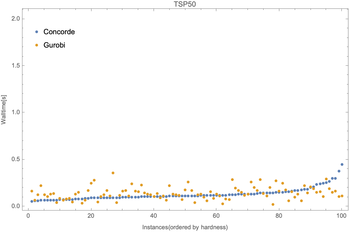
Figure 15: Concorde v.s. Gurobi on TSP50

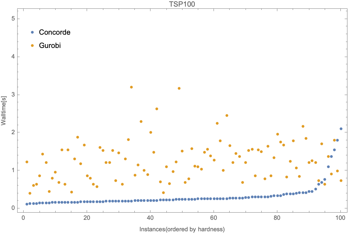
Figure 16: Concorde v.s. Gurobi on TSP100

Figure 1 and Figure 3 show the testing result of the models trained on TSP10 and TSP15, respectively. The analytical result is also shown in Table 1 and Table 2. Note that since some instances are much harder than others, we divide the data by the wall-time needed for SCIP and do a detailed comparison. Also, we compare the performance between Concorde and the TSP solving API provided by Gurobi in Figure 15 and Figure 16. The result is similar when the TSP size is small, so we didn’t include the Gurobi result in the following plots.

Test Size	Avg. Walltime(s)		Avg. Improvement(s)			Avg. Improvement(%)
	SCIP	GCNN	All	First 80	Last 20	All	First 80	Last 20
TSP10	$0.507$\mathrm{s}$$	$0.484$\mathrm{s}$$	$0.022$\mathrm{s}$$	$0.012$\mathrm{s}$$	$0.063$\mathrm{s}$$	$4.40\%$	$3.41\%$	$5.68\%$
TSP15	$2.932$\mathrm{s}$$	$2.764$\mathrm{s}$$	$0.168$\mathrm{s}$$	$0.090$\mathrm{s}$$	$0.481$\mathrm{s}$$	$5.73\%$	$5.77\%$	$5.71\%$
TSP20	$50.794$\mathrm{s}$$	$44.972$\mathrm{s}$$	$5.822$\mathrm{s}$$	$0.985$\mathrm{s}$$	$25.174$\mathrm{s}$$	$11.46\%$	$7.14\%$	$12.66\%$
TSP25	$238.699$\mathrm{s}$$	$231.872$\mathrm{s}$$	$6.827$\mathrm{s}$$	$3.527$\mathrm{s}$$	$20.028$\mathrm{s}$$	$2.86\%$	$6.52\%$	$2.05\%$

Table 1: Model Trained on TSP10

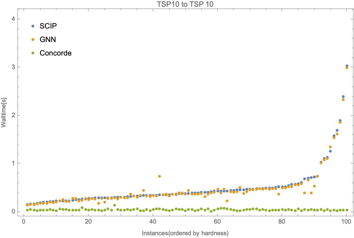
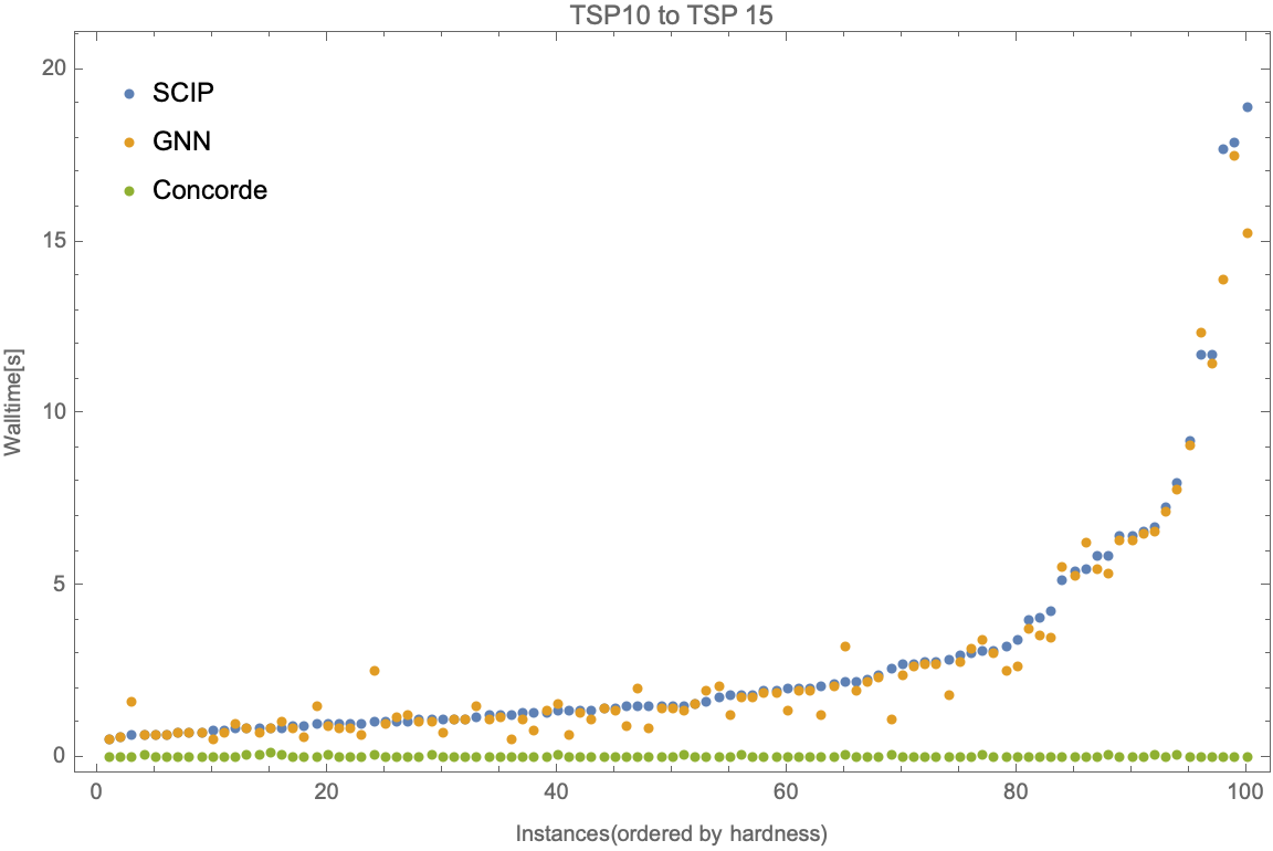
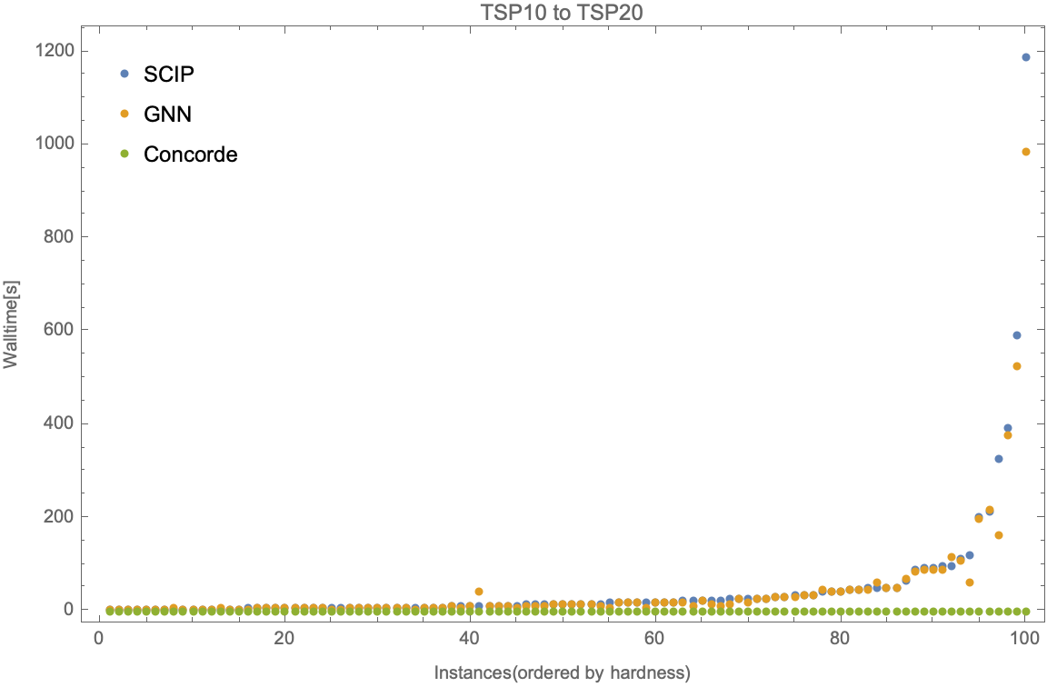
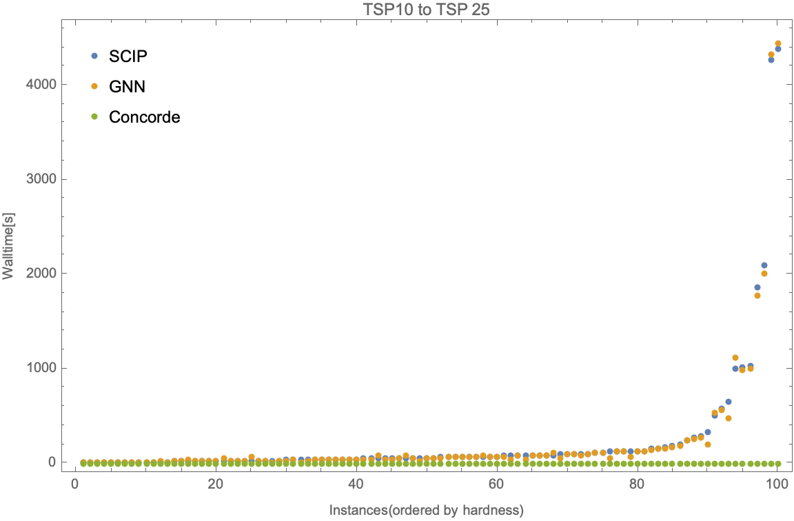
Figure 1: Result of model trained on TSP10 generalizes to TSP with various sizes.

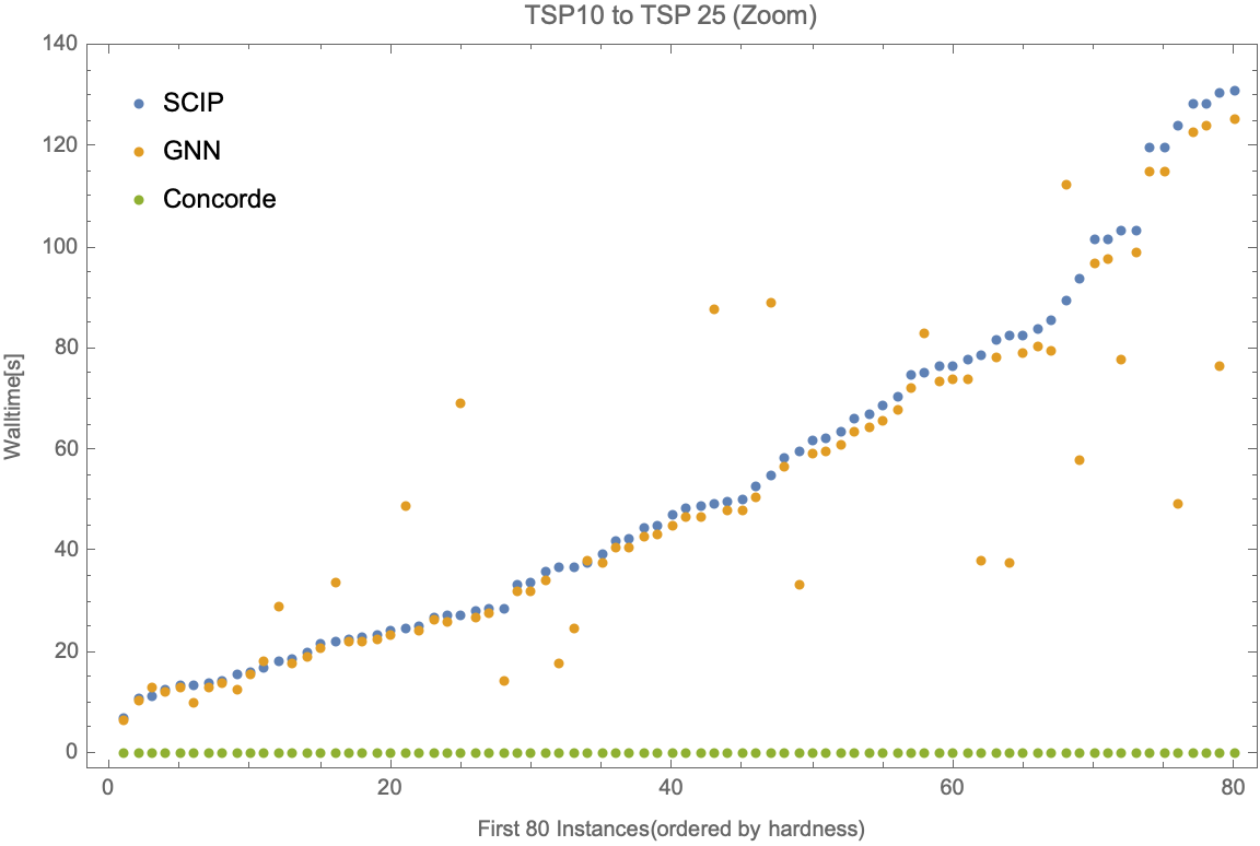
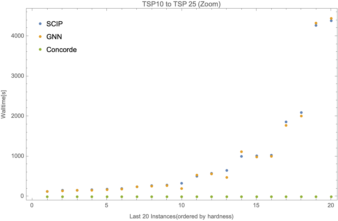
Figure 2: Result of model trained on TSP10 generalizes to TSP25 with zoomed-in.

Test Size	Avg. Walltime(s)		Avg. Improvement(s)			Avg. Improvement(%)
	SCIP	GCNN	All	First 80	Last 20	All	First 80	Last 20
TSP10	$0.490$\mathrm{s}$$	$0.461$\mathrm{s}$$	$0.028$\mathrm{s}$$	$0.020$\mathrm{s}$$	$0.063$\mathrm{s}$$	$5.80\%$	$5.60\%$	$6.07\%$
TSP15	$2.822$\mathrm{s}$$	$2.661$\mathrm{s}$$	$0.161$\mathrm{s}$$	$0.050$\mathrm{s}$$	$0.605$\mathrm{s}$$	$5.70\%$	$3.31\%$	$7.48\%$
TSP20	$49.020$\mathrm{s}$$	$47.181$\mathrm{s}$$	$1.8389$\mathrm{s}$$	$0.878$\mathrm{s}$$	$5.683$\mathrm{s}$$	$3.75\%$	$6.58\%$	$2.96\%$
TSP25	$256.253$\mathrm{s}$$	$239.864$\mathrm{s}$$	$16.389$\mathrm{s}$$	$3.515$\mathrm{s}$$	$67.886$\mathrm{s}$$	$6.40\%$	$6.56\%$	$6.36\%$

Table 2: Model Trained on TSP15

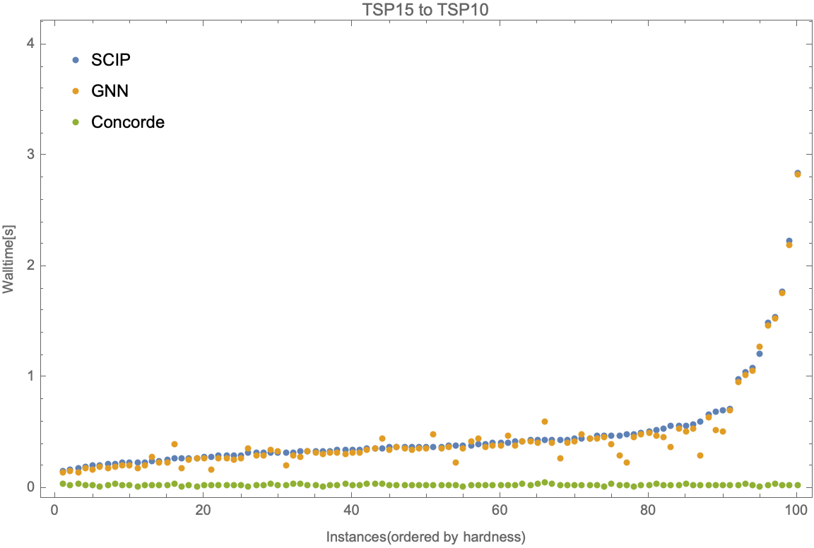
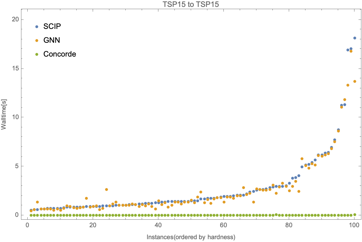
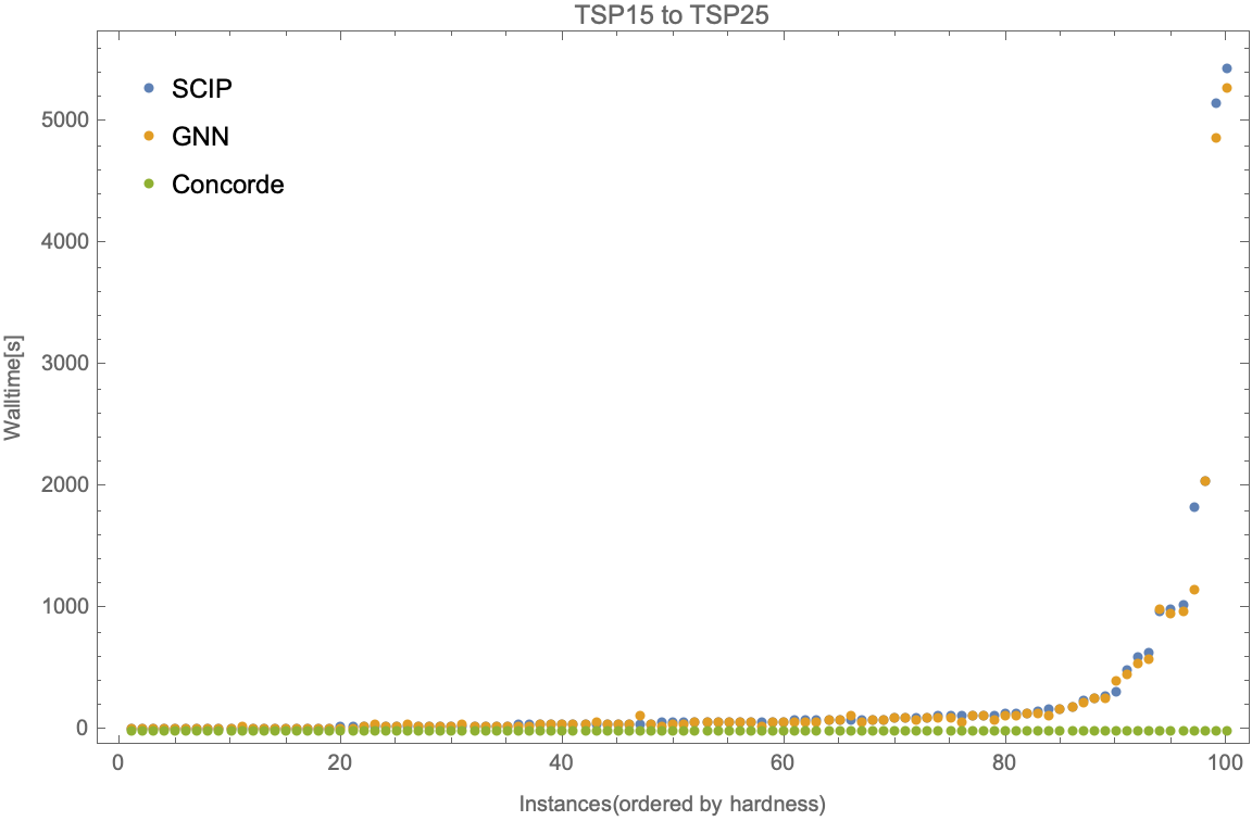
Figure 3: Result of model trained on TSP15 generalizes to TSP with various sizes.

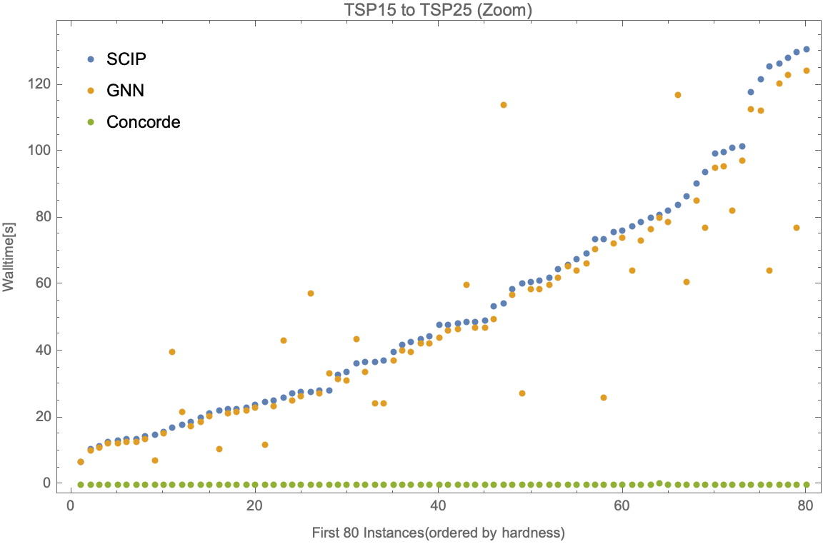
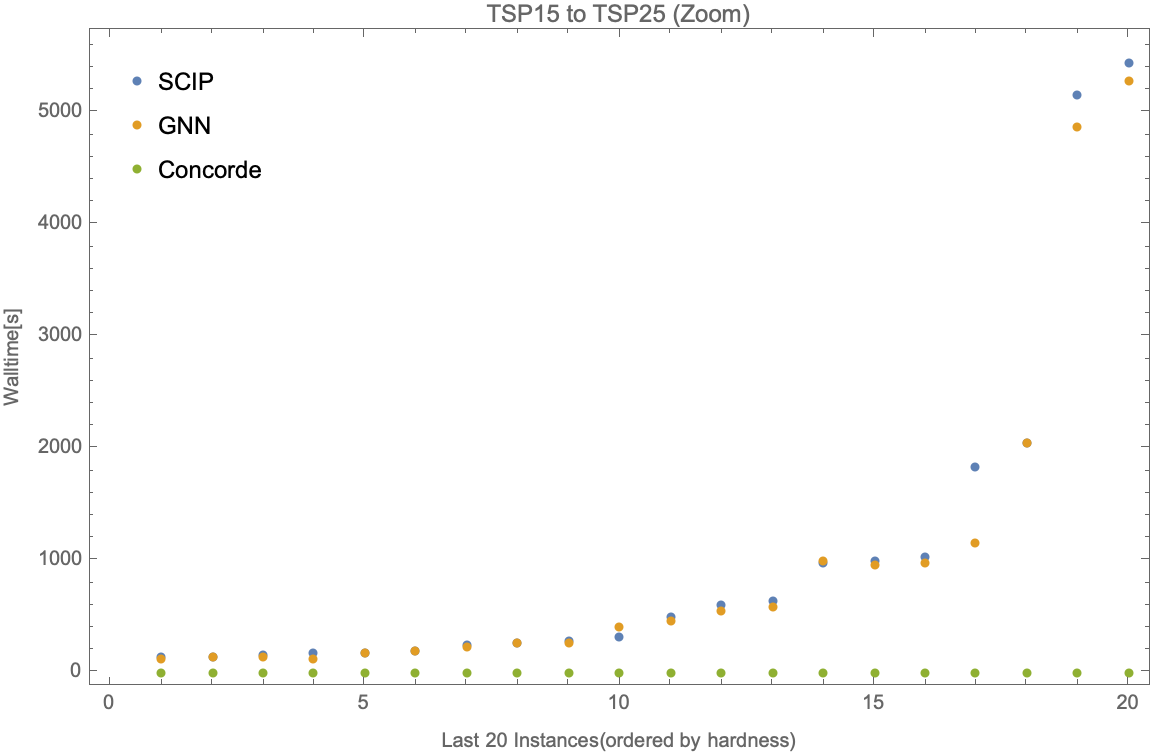
Figure 4: Result of model trained on TSP15 generalizes to TSP25 with zoomed-in.

The zoomed-in plots for other cases can be found in Section A.1 and Section A.2.

7 Discussion

7.1 Generalization Ability

We observe that our TSP10 and TSP15 imitation models outperform the SCIP solver on baseline test instances, and successfully generalizes to TSP15, TSP20, and TSP25. They perform significantly better on average than SCIP in difficult-to-solve TSPs as compared to easier instances. They also perform better in cases of larger test instances like TSP20 and TSP25 as compared to TSP10 and TSP15. This might be due to an inherent subset structure between TSP10 and TSP20 instances, and similarly TSP15 and TSP25 instances which might not be the case for smaller test sizes. Unlike other problems, when we formulate TSP as an ILP, the problem size is growing quadratically. In other words, when we look at the model performance, the generalization ability from TSP10 to TSP25 is not a $2.5\times$, but rather a $6\times$ generalization in our formulation. By adopting this methodology on a more sophisticated algorithm that formulates TSP linearly, the generalization ability should remain and the performance will be even better in terms of TSP sizes.

Recent works on finding sub-optimal solutions of TSPs, have not been able to generalize well to large test instances [17]. Generalization ability is one of the most significant properties of Combinatorial Optimization algorithms due to the increasing computational complexity when the problem size scales up. Finding a sub-optimal solution may be undesirable in a lot of real-world applications since there is no guarantee on the approximation ratio of all machine learning approaches. Hence, our work is a vital step in this direction.

7.2 Bottlenecks and Future Work

There is a huge performance difference between our proposed model (also SCIP) and the SOTA TSP solver, Concorde. Since the proposed model’s backbone is the branch and bound algorithm, by formulating TSP into an ILP, we lost some useful problem structures which can be further exploited by algorithms used in Concorde. But the existence of a similar pattern of growth in solving time for more difficult instances of larger TSP sizes even for Gurobi and Concorde is promising (see Section A.3), as our imitation model applied to these solvers should lead to similar time improvements. A major bottleneck is that SOTA solvers like Gurobi, or Concorde, are often licensed, hence not open-sourced [14, 9]. This results in the difficulty of utilizing a stronger baseline and learning from which to get further improvement.

On the other hand, the imitation method can be readily adapted to other algorithms where sequential decision-making is part of the optimization process. One promising avenue would be a direct adaption to cutting plane methods. However, this might be difficult as modern solvers usually utilize different techniques interchangeably, which makes a direct adaption non-trivial.

Another concern is that the hyperparameters are not being cross-validated. This is essentially due to computational and hardware limitations. We can increase the entropy reward when calculating cross-entropy for instances, which will motivate the model to be more active when searching for the optimum on the loss surface. We can also let SCIP use a strong branch with different probabilities, the converging rate may change and can affect the performance as well.

8 Conclusion

Finding exact solutions to combinatorial optimization problems as fast as possible is a challenging avenue in modern theoretical CS. Our proposed method is a step toward this goal via machine learning. For nearly all exact optimization solving algorithms, there is some kind of exhaustion going on which usually involves decision-making when executing the algorithm. For example, the cutting plane algorithm [12, 19] also involves decision-making on variables when it needs to choose a variable to cut. We see that by using our model to replace several such algorithms, we can speed up the inference time while still retaining a high-quality decision strategy. Furthermore, our experimental results show that the model can effectively learn such strategies while using less time when inference, which is a promising strategy when applied to other such algorithms.

Appendix A Additional Experimental Results

A.1 Model Trained on TSP10

A.1.1 Full Size Plots

We include the full-size plots for the testing result on the model trained with TSP10.

Figure 5: Test on TSP10

Figure 6: Test on TSP15

Figure 7: Test on TSP20

Figure 8: Test on TSP25

A.1.2 Zoom In Plots

We include the zoom-in plots for the testing result on the model trained with TSP10.

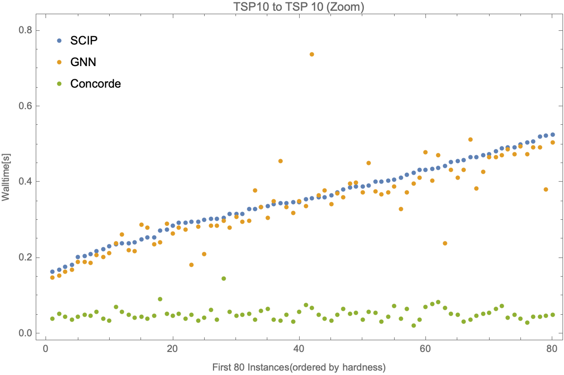
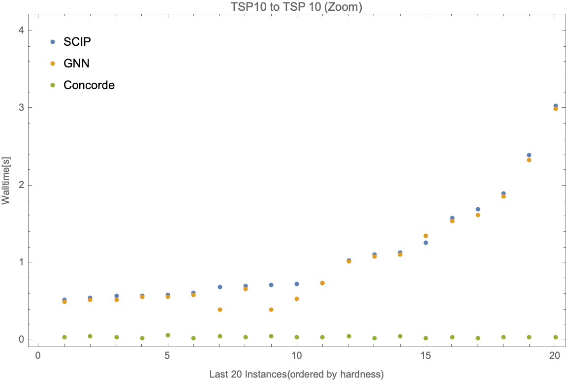
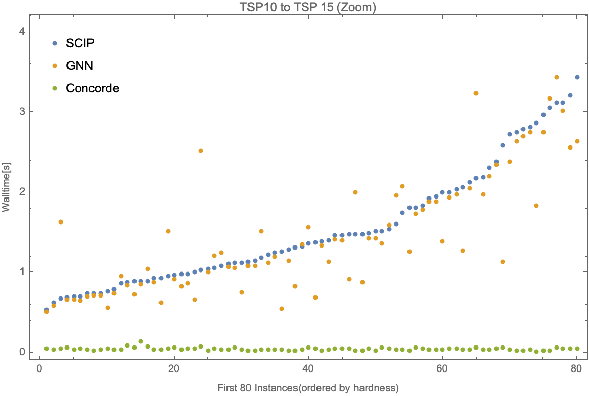
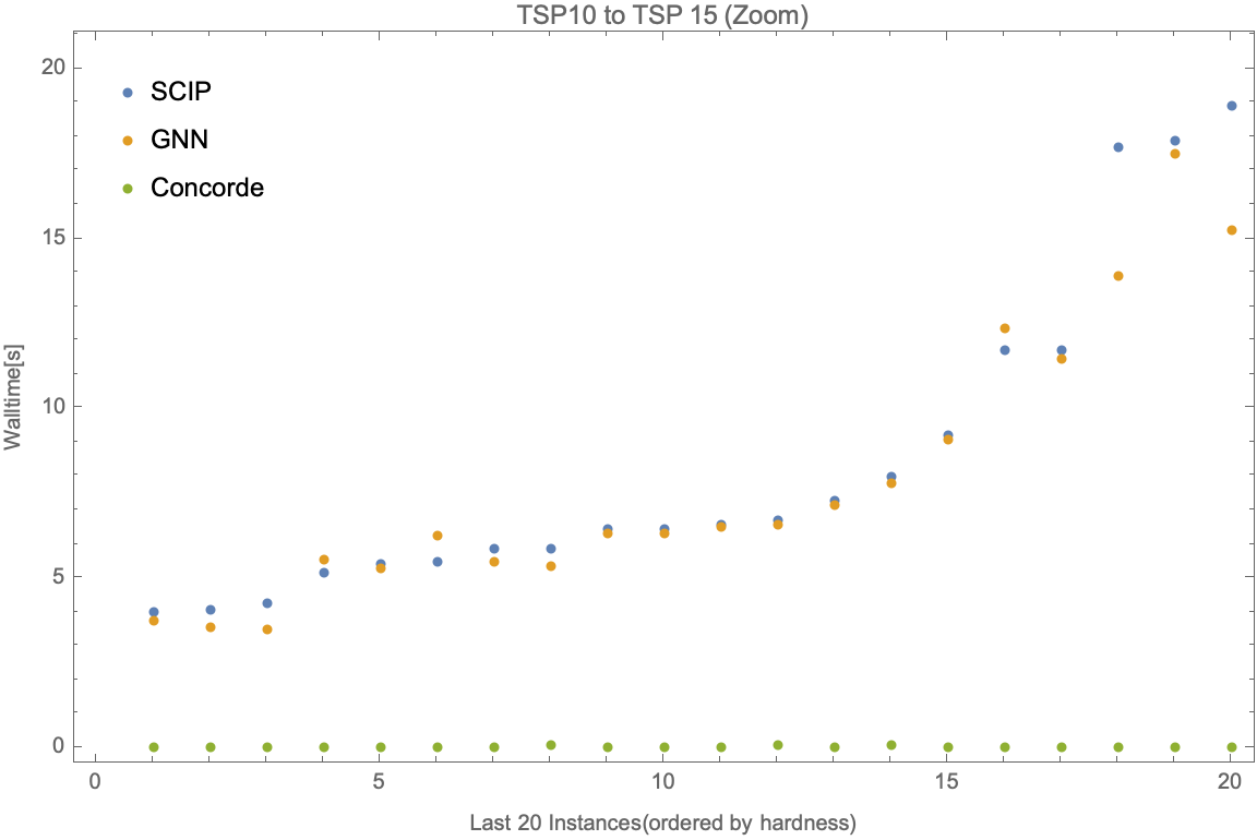
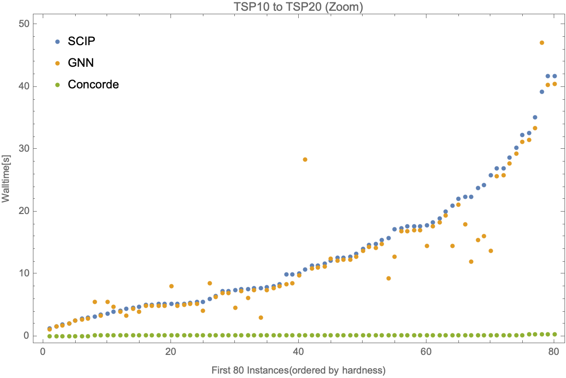
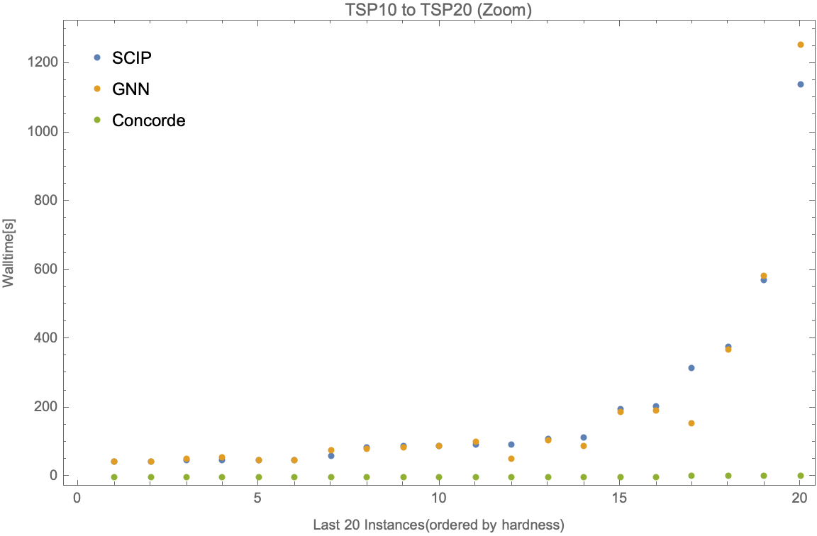
Figure 9: Result of model trained on TSP10 generalizes to TSP with various sizes with zoomed-in.

A.2 Model Trained on TSP15

A.2.1 Full Size Plots

We include the full-size plots for the testing result on the model trained with TSP15.

Figure 10: Test on TSP10

Figure 11: Test on TSP15

Figure 12: Test on TSP20

Figure 13: Test on TSP25

A.2.2 Zoom In Plots

We include the zoom-in plots for the testing result on the model trained with TSP15.

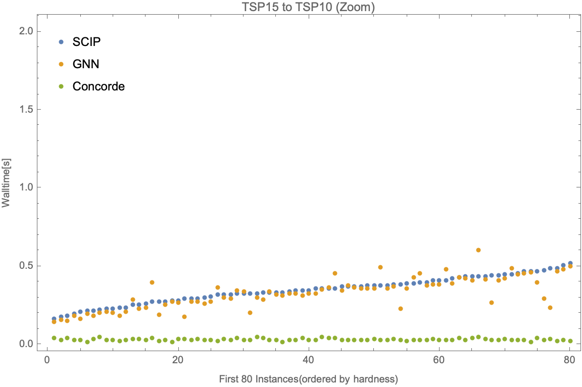
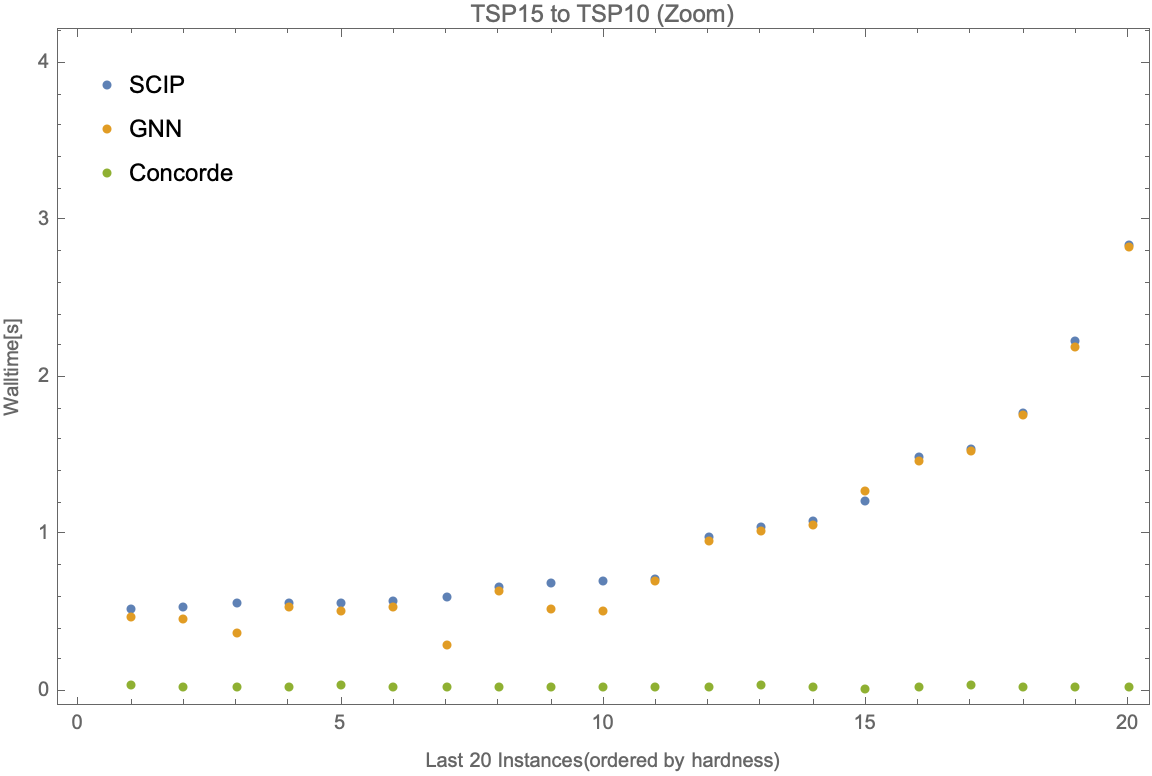
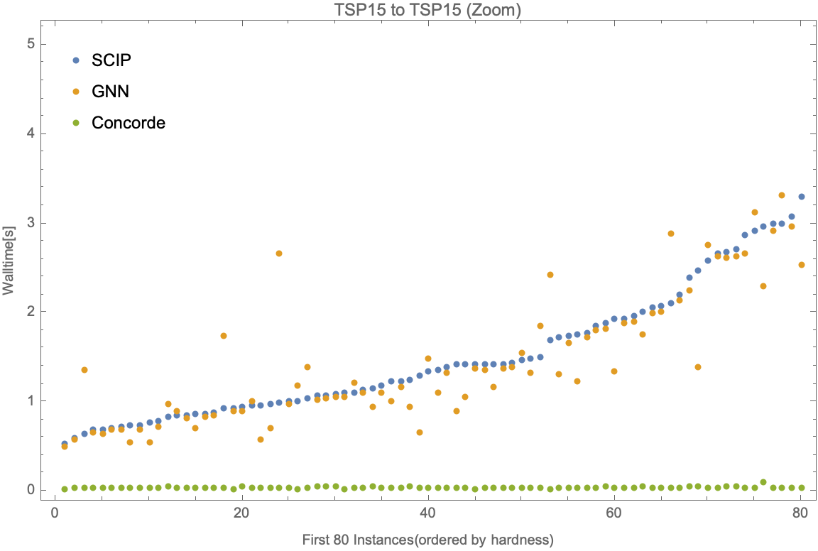
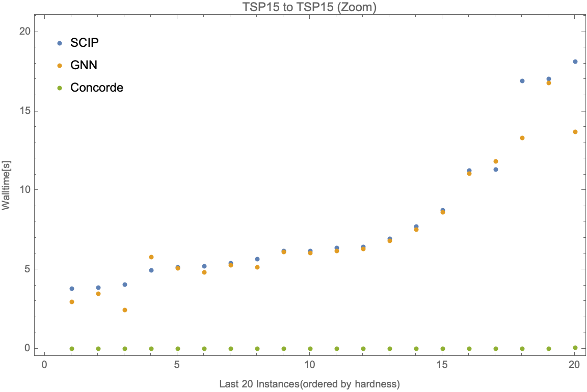
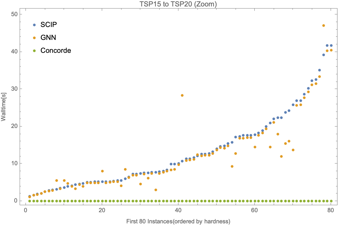
Figure 14: Result of model trained on TSP15 generalizes to TSP with various sizes with zoomed-in.

A.3 Comparison between Gurobi and Concorde

As a sanity check, we compare the performance between Concorde and the TSP API provided by Gurobi.

References

- Achterberg and Berthold [2009] Tobias Achterberg and Timo Berthold. Hybrid branching. pages 309–311, 05 2009. ISBN 978-3-642-01928-9. doi: 10.1007/978-3-642-01929-6_23.
- Achterberg and Wunderling [2013] Tobias Achterberg and Roland Wunderling. Mixed Integer Programming: Analyzing 12 Years of Progress, pages 449–481. Springer Berlin Heidelberg, Berlin, Heidelberg, 2013. ISBN 978-3-642-38189-8. doi: 10.1007/978-3-642-38189-8_18. URL https://doi.org/10.1007/978-3-642-38189-8_18.
- Achterberg et al. [2005] Tobias Achterberg, Thorsten Koch, and Alexander Martin. Branching rules revisited. Operations Research Letters, 33(1):42–54, 2005. ISSN 0167-6377. doi: https://doi.org/10.1016/j.orl.2004.04.002. URL https://www.sciencedirect.com/science/article/pii/S0167637704000501.
- Applegate et al. [1995] D. Applegate, R. Bixby, V. Chvatal, and B. Cook. Finding cuts in the tsp (a preliminary report). Technical report, 1995.
- Bestuzheva et al. [2021] Ksenia Bestuzheva, Mathieu Besançon, Wei-Kun Chen, Antonia Chmiela, Tim Donkiewicz, Jasper van Doornmalen, Leon Eifler, Oliver Gaul, Gerald Gamrath, Ambros Gleixner, Leona Gottwald, Christoph Graczyk, Katrin Halbig, Alexander Hoen, Christopher Hojny, Rolf van der Hulst, Thorsten Koch, Marco Lübbecke, Stephen J. Maher, Frederic Matter, Erik Mühmer, Benjamin Müller, Marc E. Pfetsch, Daniel Rehfeldt, Steffan Schlein, Franziska Schlösser, Felipe Serrano, Yuji Shinano, Boro Sofranac, Mark Turner, Stefan Vigerske, Fabian Wegscheider, Philipp Wellner, Dieter Weninger, and Jakob Witzig. The SCIP Optimization Suite 8.0. Technical report, Optimization Online, December 2021. URL http://www.optimization-online.org/DB_HTML/2021/12/8728.html.
- Bresson and Laurent [2021] Xavier Bresson and Thomas Laurent. The transformer network for the traveling salesman problem. ArXiv, abs/2103.03012, 2021.
- Bruna et al. [2013] Joan Bruna, Wojciech Zaremba, Arthur Szlam, and Yann LeCun. Spectral networks and locally connected networks on graphs, 2013. URL https://arxiv.org/abs/1312.6203.
- Cplex [2009] IBM ILOG Cplex. V12. 1: User’s manual for cplex. International Business Machines Corporation, 46(53):157, 2009.
- David Applegate and Robert Bixby and Vasek Chvátal and William Cook [2022] David Applegate and Robert Bixby and Vasek Chvátal and William Cook. Concorde-03.12.19, 2022. URL http://www.math.uwaterloo.ca/tsp/concorde/downloads/downloads.htm.
- Fischetti and Monaci [2012] Matteo Fischetti and Michele Monaci. Branching on nonchimerical fractionalities. Operations Research Letters, 40:159–164, 05 2012. doi: 10.1016/j.orl.2012.01.008.
- Gasse et al. [2019] Maxime Gasse, Didier Chételat, Nicola Ferroni, Laurent Charlin, and Andrea Lodi. Exact combinatorial optimization with graph convolutional neural networks. In Advances in Neural Information Processing Systems 32, 2019.
- Gilmore and Gomory [1961] R Gilmore and Ralph Gomory. A linear programming approach to the cutting stock problem i. Oper Res, 9, 01 1961. doi: 10.1287/opre.9.6.849.
- Gori et al. [2005] Marco Gori, Gabriele Monfardini, and Franco Scarselli. A new model for learning in graph domains. Proceedings. 2005 IEEE International Joint Conference on Neural Networks, 2005., 2:729–734 vol. 2, 2005.
- Gurobi Optimization, LLC [2022] Gurobi Optimization, LLC. Gurobi Optimizer Reference Manual, 2022. URL https://www.gurobi.com.
- Howard [1960] R.A. Howard. Dynamic programming and Markov processes. Technology Press of Massachusetts Institute of Technology, 1960. URL https://books.google.com/books?id=fXJEAAAAIAAJ.
- Hussein et al. [2017] Ahmed Hussein, Mohamed Medhat Gaber, Eyad Elyan, and Chrisina Jayne. Imitation learning: A survey of learning methods. ACM Comput. Surv., 50(2), apr 2017. ISSN 0360-0300. doi: 10.1145/3054912. URL https://doi.org/10.1145/3054912.
- Joshi et al. [2019] Chaitanya K. Joshi, Thomas Laurent, and Xavier Bresson. An efficient graph convolutional network technique for the travelling salesman problem, 2019. URL https://arxiv.org/abs/1906.01227.
- Linderoth and Savelsbergh [1999] Jeff T. Linderoth and Martin W. P. Savelsbergh. A computational study of search strategies for mixed integer programming. INFORMS J. Comput., 11(2):173–187, 1999. doi: 10.1287/ijoc.11.2.173. URL https://doi.org/10.1287/ijoc.11.2.173.
- Marchand et al. [2002] Hugues Marchand, Alexander Martin, Robert Weismantel, and Laurence Wolsey. Cutting planes in integer and mixed integer programming. Discrete Applied Mathematics, 123(1):397–446, 2002. ISSN 0166-218X. doi: https://doi.org/10.1016/S0166-218X(01)00348-1. URL https://www.sciencedirect.com/science/article/pii/S0166218X01003481.
- Miller et al. [1960] C. E. Miller, A. W. Tucker, and R. A. Zemlin. Integer programming formulation of traveling salesman problems. J. ACM, 7(4):326–329, oct 1960. ISSN 0004-5411. doi: 10.1145/321043.321046. URL https://doi.org/10.1145/321043.321046.
- Paschos [2014] V.T. Paschos. Applications of Combinatorial Optimization. ISTE. Wiley, 2014. ISBN 9781119015222. URL https://books.google.com/books?id=qmVEBAAAQBAJ.
- Patel and Chinneck [2007] Jagat Patel and John Chinneck. Active-constraint variable ordering for faster feasibility of mixed integer linear programs. Math. Program., 110:445–474, 09 2007. doi: 10.1007/s10107-006-0009-0.
- Pomerleau [1991] Dean A. Pomerleau. Efficient training of artificial neural networks for autonomous navigation. Neural Computation, 3(1):88–97, 1991. doi: 10.1162/neco.1991.3.1.88.
- Prouvost et al. [2020] Antoine Prouvost, Justin Dumouchelle, Lara Scavuzzo, Maxime Gasse, Didier Chételat, and Andrea Lodi. Ecole: A gym-like library for machine learning in combinatorial optimization solvers. In Learning Meets Combinatorial Algorithms at NeurIPS2020, 2020. URL https://openreview.net/forum?id=IVc9hqgibyB.
- Sutton and Barto [2018] R.S. Sutton and A.G. Barto. Reinforcement Learning, second edition: An Introduction. Adaptive Computation and Machine Learning series. MIT Press, 2018. ISBN 9780262352703. URL https://books.google.com/books?id=uWV0DwAAQBAJ.
- Wolsey [2020] Laurence Wolsey. Branch and Bound, chapter 7, pages 113–138. John Wiley and Sons, Ltd, 2020. ISBN 9781119606475. doi: https://doi.org/10.1002/9781119606475.ch7. URL https://onlinelibrary.wiley.com/doi/abs/10.1002/9781119606475.ch7.
- Åström [1965] K.J Åström. Optimal control of markov processes with incomplete state information. Journal of Mathematical Analysis and Applications, 10(1):174–205, 1965. ISSN 0022-247X. doi: https://doi.org/10.1016/0022-247X(65)90154-X. URL https://www.sciencedirect.com/science/article/pii/0022247X6590154X.