Uncertainty-Aware Unsupervised Image Deblurring with Deep Residual Prior

Abstract

Non-blind deblurring methods achieve decent performance under the accurate blur kernel assumption. Since the kernel uncertainty (i.e. kernel error) is inevitable in practice, semi-blind deblurring is suggested to handle it by introducing the prior of the kernel (or induced) error. However, how to design a suitable prior for the kernel (or induced) error remains challenging. Hand-crafted prior, incorporating domain knowledge, generally performs well but may lead to poor performance when kernel (or induced) error is complex. Data-driven prior, which excessively depends on the diversity and abundance of training data, is vulnerable to out-of-distribution blurs and images. To address this challenge, we suggest a dataset-free deep residual prior for the kernel induced error (termed as residual) expressed by a customized untrained deep neural network, which allows us to flexibly adapt to different blurs and images in real scenarios. By organically integrating the respective strengths of deep priors and hand-crafted priors, we propose an unsupervised semi-blind deblurring model which recovers the clear image from the blurry image and inaccurate blur kernel. To tackle the formulated model, an efficient alternating minimization algorithm is developed. Extensive experiments demonstrate the favorable performance of the proposed method as compared to model-driven and data-driven methods in terms of image quality and the robustness to different types of kernel error.

1 Introduction

Image blurring is mainly caused by camera shake [28], object motion [9], and defocus [42]. By assuming the blur kernel is shift-invariant, the image blurring can be formulated as the following convolution process:

$$\bm{y}=\bm{k}\otimes\bm{x}+\bm{n},$$ (1)

where $\bm{y}$ and $\bm{x}$ denote the blurry image and the clear image respectively, $\bm{k}$ represents the blur kernel, $\bm{n}$ represents the additive Gaussian noise, and $\otimes$ is the convolution operator. To acquire the clear image from the blurry one, image deblurring has received considerable research attention and related methods have been developed.

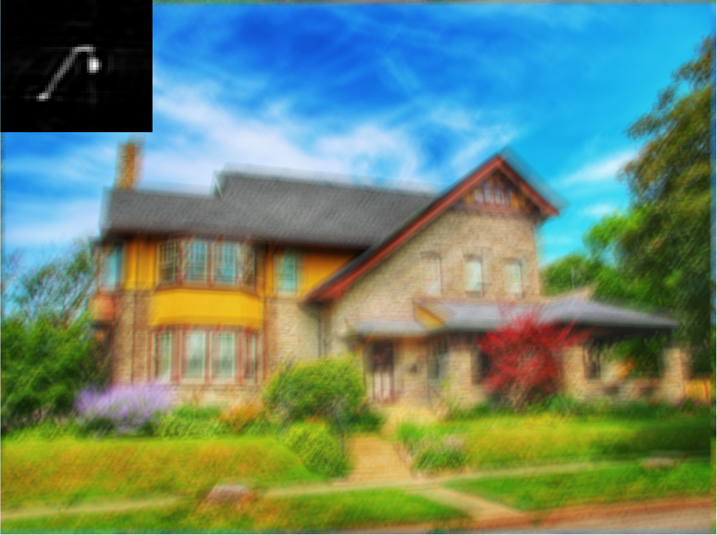
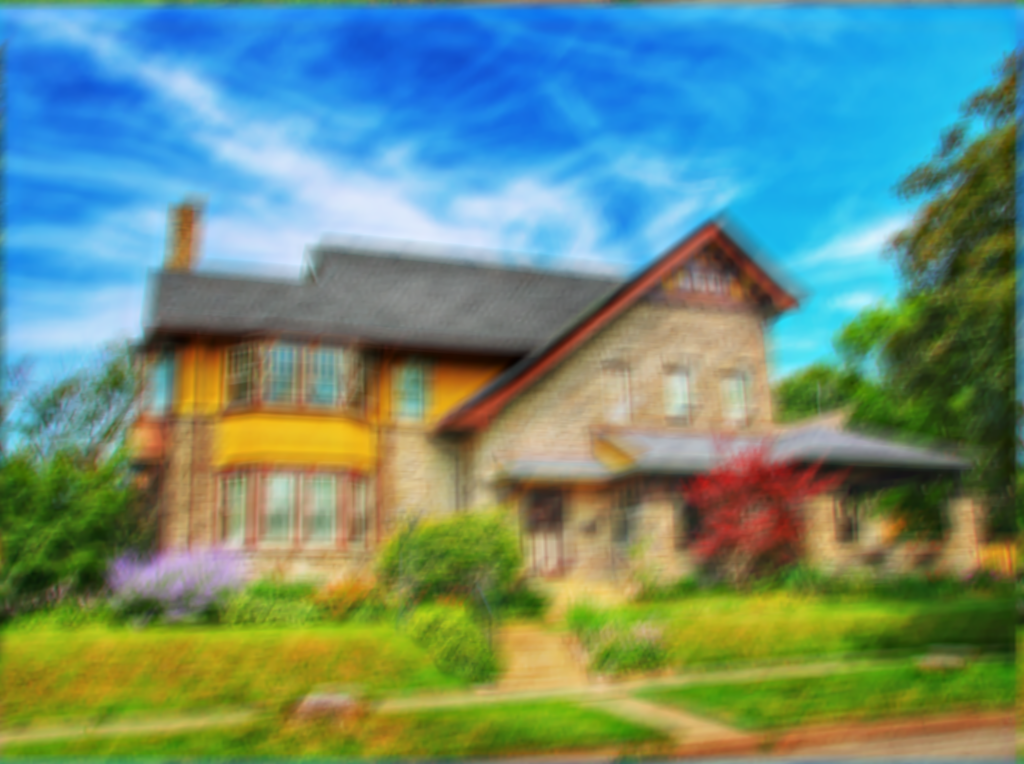
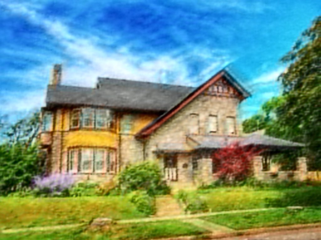
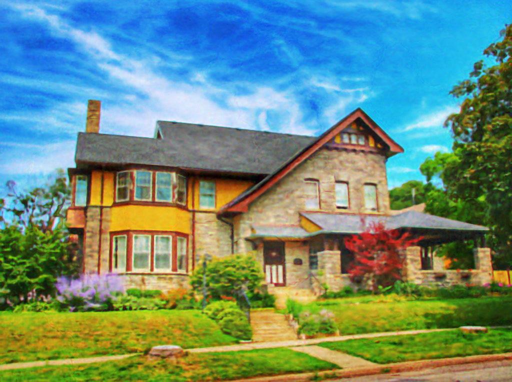
Blurry	[8]	[34]	Ours
PSNR 19.56	PSNR 20.83	PSNR 22.75	PSNR 25.66
True Res.	Res. in [8]	Res. in [34]	Our Res.
MSE 0	MSE 0.075	MSE 0.067	MSE 0.027

Figure 1: Visual comparison of the restored results and estimated residuals by three semi-blind methods based on different priors for the residual induced by the kernel error, including hand-crafted prior [8], data-driven prior [34], and the proposed deep residual prior (DRP). The true residual is the convolution result of the kernel error and the clear image ($\bm{r}=\Delta\bm{k}\otimes\bm{x}$). The closer estimated residual is to the true residual, the better it is.

In terms of the availability of kernel, current image deblurring methods can be mainly classified into two categories, i.e., blind deblurring methods in which the blur kernel is assumed to be unknown, and non-blind deblurring methods in which the blur kernel is assumed to be known or computed elsewhere. Typical blind deblurring methods [13, 17, 32, 21, 27, 31, 38, 18, 43, 15] involve two steps: 1) estimating the blur kernel from the blurry images, and 2) recovering the clear image with the estimated blur kernel. Recently there also emerge transformer-based [39, 36] and unfolding networks [19] that learn direct mappings from blurry image to the deblurred one without using the kernel. Non-blind deblurring methods [35, 11, 5, 40, 6, 1, 4, 22], based on various priors for the clear image, estimate the clear image solely from the blurry image with known blur kernel. Notably, existing non-blind deblurring methods can perform well under the error-free kernel assumption. However, in the real application, uncertainty exists in the kernel acquisition process. As a result, these methods without handling kernel uncertainty often introduce artifacts and cause unpleasant performances.

Recently, semi-blind methods are suggested to handle kernel uncertainty by introducing the prior for the kernel (or induced) error. In the literature, there are two groups of priors of kernel (or induced) error, i.e., hand-crafted priors and data-driven priors. Hand-crafted priors [8, 41], incorporating domain knowledge, generally perform well but may lead to poor performance when the distribution of kernel (or induced) error is complex. For example, hand-crafted priors (e.g., sparse prior [8]) are relatively impotent to characterize the complex intrinsic structure of the kernel induced error; see Figure 1. Data-driven priors [34, 20, 26], which excessively depend on the diversity and abundance of training data, are vulnerable to out-of-distribution blurs and images. Specifically, the data-driven prior in [34] that is expressed by a trained network introduces artifacts around the sharp edges; see Figure 1. Therefore, how to design a suitable prior for the kernel (or induced) error remains challenging.

To address this problem, we suggest a dataset-free deep prior called deep residual prior (DRP) for the kernel induced error (termed as residual), which leverages the strong representation ability of deep neural networks. Specifically, DRP is expressed by an untrained customized deep neural network. Moreover, by leveraging the general domain knowledge, we use the sparse prior to guide DRP to form a semi-blind deblurring model. This model organically integrates the respective strengths of deep priors and hand-crafted priors to achieve favorable performance. To the best of our knowledge, we are the first to introduce the untrained network to capture the kernel induced error in semi-blind problems, which is a featured contribution of our work.

In summary, our contributions are mainly three-fold:

$\bullet$ For the residual induced by the kernel uncertainty, we elaborately design a dataset-free DRP, which allows us to faithfully capture the complex residual in real-world applications as compared to hand-crafted priors and data-driven priors.

$\bullet$ Empowered by the deep residual prior, we suggest an unsupervised semi-blind deblurring model by synergizing the respective strengths of dataset-free deep prior and hand-crafted prior, which work togerther to deliver promising results.

$\bullet$ Extensive experiments on different blurs and images sustain the favorable performance of our method, especially for the robustness to kernel error.

2 Related Work

This section briefly introduces literatures on semi-blind deblurring methods that focus on handling the kernel error.

In the early literature of semi-blind deblurring, model-driven methods are dominating, in which these methods generally handle the kernel uncertainty with some hand-crafted priors. For example, Zhao et al. [41] directly treated the kernel error as additive zero-mean white Gaussian noise (AWGN), and $l_{2}$-regularizer is utilized to model it. Ji and Wang [8] treated the residual as an additional variable to be estimated, and a sparse constraint in the spatial domain is utilized to regularize it (i.e., $l_{1}$-regularizer). However, such hand-crafted priors, which are based on certain statistical distribution assumptions (such as sparsity and AWGN), are not sufficient to characterize the complex structure of kernel error. Thus, such methods are efficient sometimes but not flexible enough to handle the kernel error in complex real scenarios.

Recently, triggered by the expressing power of neural networks, many deep learning-based methods [25, 30, 34, 20, 26] have emerged, in which data-driven priors are learned from a large number of external data for handling kernel error. The key of these methods is to design an appropriate neural network structure and learning pipeline. For instance, Ren et al.  [25] suggested a partial deconvolution model to explicitly model kernel estimation error in the Fourier domain. Vasu et al. [34] trained their convolutional neural networks with a large number of real and synthetic noisy blur kernels to achieve good performance for image deblurring with inaccurate kernels. Ren et al. [26] suggested simultaneously learning the data and regularization term to tackle the image restoration task with an inaccurate degradation model. Nan and Ji [20] cleverly unrolled an iterative total-least-squares estimator in which the residual prior is learned by a customized dual-path U-Net. This method well handles kernel uncertainty and achieves remarkable deblurring performance in a supervised manner. Although these methods achieve decent performances in certain cases, they excessively depend on the diversity and abundance of training data and are vulnerable to out-of-distribution blurs and images.

(a)	(b)	(c)	(d)

Figure 2: Visualization of the residual induced by the kernel error. (a) Clear image. (b) Blurry image with the true kernel (motion blur with a length of 150 pixels and orientation of 20^∘). (c) Blurry image with the inaccurate kernel (motion blur with a length of 150 pixels and orientation of 40^∘). (d) The residual induced by kernel error which is the difference between (b) and (c).

3 Proposed Method

In this paper, we propose a dataset-free deep prior for the residual expressed by a customized untrained deep neural network, which allows us to flexibly adapt to different blurs and images in real scenarios. By organically integrating the respective strengths of deep priors and hand-crafted priors, we propose an unsupervised semi-blind deblurring model which recovers the clear image from the blurry image and blur kernel.

3.1 Problem Formulation

We first take a look at the formulation of the semi-blind deblurring problem. Considering the kernel error and possible artifacts, we formulate the degradation process as

$$\bm{y} =(\bm{\widehat{k}}+\Delta\bm{k})\otimes\bm{x}+\bm{h}+\bm{n}=\bm{\widehat{k}}\otimes\bm{x}+\bm{r}+\bm{h}+\bm{n},$$ (2)

where $\bm{y}$ and $\bm{x}$ denote the blurry image and clear image respectively, $\bm{\widehat{k}}$ and $\Delta\bm{k}$ represent the inaccurate blur kernel and kernel error, $\bm{n}$ represents the AWGN, $\otimes$ is the convolution operator, $\bm{r}=\Delta\bm{k}\otimes\bm{x}$ is the residual induced by the kernel error, and $\bm{h}$ represents the artifacts.

3.2 Mathematical Model

Note that deriving $\bm{x}$, $\bm{h}$, and $\bm{r}$ from the blurry image $\bm{y}$ is a typical ill-posed problem which admits infinite solutions. To confine the solution space, prior information of $\bm{x}$, $\bm{h}$, and $\bm{r}$ is required. In this work, we utilize the proposed DRP incorporated with the sparse prior for the residual $\bm{r}$, deep image prior (DIP) [33] incorporated with total variation for the clear image $\bm{x}$, and the sparse prior in the discrete cosine transform (DCT) domain for the artifact $\bm{h}$. The motivations are as follows.

Deep Residual Prior and Sparse Prior in the Spatial Domain for $\bm{r}$. We utilize the DRP guided by the sparse prior in the spatial domain to model the residual $\bm{r}$. Since the intrinsic structures of residual are complex and diverse, it is hard to model the residual accurately by hand-crafted priors or data-driven priors. The dataset-free prior expressed by an untrained neural network becomes a natural choice to flexibly and robustly model the complex residuals. To this end, we propose the dataset-free DRP expressed by a tailored untrained network—the customized U-Net to capture the residual $\bm{r}$. On the other hand, in the spatial domain the residual is generally sparse; see Figure 2. Based on this observation, the sparse prior in the spatial domain is utilized as the domain knowledge to guide DRP. These two priors are organically combined to better characterize the complex residual $\bm{r}$.

Deep Image Prior and Total Variation Prior for $\bm{x}$. We utilize DIP guided by total variation prior to model the clear image $\bm{x}$. Since DIP [33, 24] exploits the statistics of clear image by the structure of an untrained convolutional neural network, it is suitable to model different blurs and images in a zero-shot scenario. On the other hand, to enforce the local smoothness of clear image, we use total variation prior to guide DIP. These two priors are organically combined to better model the clear image $\bm{x}$. The effectiveness of this combination is verified in the work [24].

Sparse Prior in the DCT Domain for $\bm{h}$. We utilize the sparse prior in the DCT domain for modeling the artifacts $\bm{h}$. It is worth noting that the artifacts $\bm{h}$ caused by the kernel error $\Delta\bm{k}$ generally have strong periodicity around the sharp edges. This indicates that its DCT coefficient $\bm{v}=\mathcal{C}\bm{h}$ ($\mathcal{C}$ is the DCT operator) is sparse [8], and it is reasonable to consider sparse prior for artifacts $\bm{h}$ in the DCT domain.

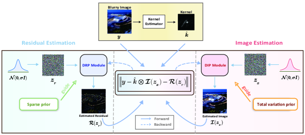
Figure 3: The diagram of the proposed model. The DIP module estimates the image $\mathcal{I}_{\bm{\theta}}(\bm{z_{x}})$ from random noise input $\bm{z_{x}}$ and the DRP module estimates the residual $\mathcal{R}_{\bm{\theta}}(\bm{z_{r}})$ from random noise input $\bm{z_{r}}$.

Following the above arguments, we propose the following unsupervised semi-blind deblurring model (see Figure 3 for the diagram). The corresponding optimization problem can be formulated as follows:

$$\mathop{{\min}}_{\bm{\theta},\bm{\zeta},\bm{v}} \left\|\bm{y}-\bm{\widehat{k}}\otimes\mathcal{I}_{\bm{\theta}}(\bm{z_{x}})-\mathcal{R}_{\bm{\zeta}}(\bm{z_{r}})-\mathcal{C}^{T}\bm{v}\right\|_{F}^{2}$$

$$+ \lambda_{1}\|\mathcal{I}_{\bm{\theta}}(\bm{z_{x}})\|_{\text{TV}}+\lambda_{2}\|\mathcal{R}_{\bm{\zeta}}(\bm{z_{r}})\|_{1}+\lambda_{3}\|\bm{v}\|_{1},$$ (3)

where $\bm{y}\in\mathbb{R}^{n_{1}\times n_{2}}$ and $\bm{x}\in\mathbb{R}^{n_{1}\times n_{2}}$ denote the blurry image and clear image, respectively; $\bm{\widehat{k}}$ represents the inaccurate blur kernel; $\mathcal{I}_{\bm{\theta}}(\bm{z_{x}})\in\mathbb{R}^{n_{1}\times n_{2}}$ and ${\cal R}_{\bm{\zeta}}(\bm{z}_{\bm{r}})\in\mathbb{R}^{n_{1}\times n_{2}}$ are the estimates of the clear image $\bm{x}$ and the residual $\bm{r}$, which are generated from untrained neural networks $\mathcal{I}_{\bm{\theta}}(\cdot)$ and $\mathcal{R}_{\bm{\zeta}}(\cdot)$, respectively; $\bm{\theta}$ and $\bm{\zeta}$ collect the corresponding network parameters; $\bm{z}_{x}\sim\mathcal{N}(0,\sigma\bm{I})$ and $\bm{z}_{r}\sim\mathcal{N}(0,\sigma\bm{I})$ are the random inputs of the neural networks. $\|\cdot\|_{\text{TV}}$ is the total variation regularizer that can be denoted by $\|\nabla_{x}(\cdot)\|_{1}+\|\nabla_{y}(\cdot)\|_{1}$, where $\nabla_{x}$ and $\nabla_{y}$ are the difference operators. Given the inaccurate kernel and the blurry image, we can infer the clear image, residual, and artifacts in model (3) in an unsupervised manner.

In this model, the indispensable hand-crafted priors and deep priors are organicaly intergrated in the our model and work together to deliver promising results.

3.3 Alternating Minimization Algorithm

To tackle the formulated model, we suggest an alternating minimization algorithm. Since the variables are coupled, we suggest decomposing the minimization problem into two easier subproblems by the following alternating minimization scheme:

$$\{\bm{\theta}^{i+1},\bm{\zeta}^{i+1}\}\in\mathop{\arg\min}_{\bm{\theta},\bm{\zeta}}~{}\mathcal{L}\left(\bm{\theta},\bm{\zeta},{\bm{v}}^{i}\right),$$ (4)

$$\bm{v}^{i+1}=\mathop{\arg\min}_{\bm{v}}~{}\mathcal{L}\left(\bm{\theta}^{i+1},\bm{\zeta}^{i+1},\bm{v}\right),$$ (5)

where the superscript “$i$” is the iteration number and $\mathcal{L}(\bm{\theta},\bm{\zeta},\bm{v})$ is the objective function in Eqn. (3). The detailed solutions for these two subproblems are as follows.

1) {$\bm{\theta},\bm{\zeta}$}-subproblem: The $\{\bm{\theta},\bm{\zeta}\}$-subproblem (5) can be solved by using gradient-based ADAM algorithm [10]. The gradients w.r.t. $\bm{\theta}$ and $\bm{\zeta}$ can be computed by the standard back-propagation algorithm [29]. Here we jointly update the weights $\bm{\theta}$ and $\bm{\zeta}$ in an iteration.

2) $\bm{v}$-subproblem: Let

$$\mathcal{D}(\bm{\theta},\bm{\zeta},\bm{v})=\left\|\bm{y}-\bm{\widehat{k}}\otimes\mathcal{I}_{\bm{\theta}}(\bm{z_{x}})-\mathcal{R}_{\bm{\zeta}}(\bm{z_{r}})-\mathcal{C}^{T}\bm{v}\right\|_{F}^{2},$$

then the $\bm{v}$-subproblem (5) is

$$\bm{v}^{i+1}=\mathop{\arg\min}_{\bm{v}}~{}\lambda_{3}\|\bm{v}\|_{1}+\mathcal{D}(\bm{\theta}^{i+1},\bm{\zeta}^{i+1},\bm{v}),$$

which can be exactly solved by using proximal gradient descent:

$$\bm{v}^{i+1}=\mathcal{S}_{\lambda_{3}/L}\left(\bm{v}^{i}-\frac{1}{L}\nabla_{\bm{v}}\mathcal{D}(\bm{\theta}^{i+1},\bm{\zeta}^{i+1},\bm{v}^{i})\right),$$ (6)

where $L>0$ is a constant, and $\mathcal{S}_{\delta}$ is the soft-thresholding operator defined by

$$\mathcal{S}_{\delta}(\bm{a})_{ij}=\max\left(\left|a_{ij}\right|-\delta,0\right)\operatorname{sgn}\left(a_{ij}\right).$$

where $a_{ij}$ is the $(i,j)$-th entry of matrix $\bm{a}$. The overall minimization algorithm is summarized in Algorithm 1.

Algorithm 1 Alternating minimization algorithm

Input: Blurry image $\bm{y}$, inaccurate kernel $\bm{\widehat{k}}$, the parameters ${\lambda_{s}~{}(s=1,2,3)}$, and iteration number $T$.
Initailization: Random input $\bm{z}_{x}\sim\mathcal{N}(0,\sigma\bm{I})$ and $\bm{z}_{r}\sim\mathcal{N}(0,\sigma\bm{I})$.

1:  for $i=0$ to $T$ do

2:     $\widehat{\bm{x}}^{i+1}=\mathcal{I}_{\bm{\theta}^{i}}(\bm{z_{x}}),\widehat{\bm{r}}^{i+1}=\mathcal{R}_{\bm{\zeta}^{i}}(\bm{z_{r}})$;

3:     compute the gradients w.r.t $\bm{\theta}$ and $\bm{\zeta}$;

4:     jointly update $\bm{\theta}^{i+1},\bm{\zeta}^{i+1}$ using ADAM;

5:     update $\bm{v}^{i+1}$ using (6);

6:  end for

Output: the restored image $\widehat{\bm{x}}$ and the residual $\widehat{\bm{r}}.$

4 Experiments

Extensive experiments on simulated and real blurry images are reported to substantially demonstrate the effectiveness of the proposed method, especially the robustness to different types of kernel error.

4.1 Experimental Setup

• Evaluation Metrics. Following prior works of deblurring, we use the peak signal-to-noise ratio (PSNR) and structural similarity index (SSIM) to evaluate the restoration quality of the images. To evaluate the quality of residual estimation, we use the mean square error (MSE), which measures the average difference of pixels in the entire true residual and estimated residual. A lower MSE value means there is less difference between the true residual and estimated residual.

• Model Hyperparameters Setting. The model hyperparameters of the proposed method are $\{\lambda_{i}\}_{i=1}^{3}$, which are tuned to obtain best PSNR value. In our experiments, $\lambda_{1},~{}\lambda_{2},~{}\lambda_{3}$ are empirically determined to be $5\times 10^{-2},5\times 10^{-5},5\times 10^{-7}$, respectively. We also conduct the sensitivity analysis of different model hyperparameters in the supplementary materials.

• Algorithm Hyperparameters Setting. In all experiments, we set the total iteration number of the proposed algorithm to be 1500. The default learning rates of networks $\mathcal{I}_{\bm{\theta}}$ and $\mathcal{R}_{\bm{\zeta}}$ are respectively $9\times 10^{-3}$ and $5\times 10^{-4}$.

• Platform. In this work, all experiments are conducted on the PyTorch 1.10.1 and MATLAB 2017b platform with an i5-12400f CPU, RTX 3060 GPU, and 16GB RAM.

4.2 Ablation Study

The ablation studies primarily focus on two aspects: a) exploring the influence of different combinations of deep priors and hand-crafted priors; b) exploring the superiority of the customized U-Net compared to other classic architectures in capturing the residual $\bm{r}$ induced by kernel error.

4.2.1 The Influence of Different Combinations of Deep Priors and Hand-crafted Priors

Table 1: The average metric values of the restored results by reconciling different hand-crafted priors with deep priors.

Method	PSNR	SSIM
w/o sparse prior for $\bm{r}$	26.77	0.853
w/o sparse prior for $\bm{v}$	27.25	0.845
w/o total variation for $\bm{x}$	27.98	0.871
w/o DIP for $\bm{x}$	26.54	0.867
w/o DRP for $\bm{r}$	25.69	0.842
Ours	28.64	0.892

To investigate the role of different priors in our model, we perform experiments by reconciling deep priors and hand-crafted priors. The test images contain 24 blurry images that are blurred with 8 sharp images and 3 typical kernels; see supplementary materials. Table 1 lists the average metric values of the restored results by reconciling different hand-crafted priors with deep priors. We can observe from the table that the deep priors and hand-crafted priors are indispensable, working together to deliver promising results.

4.2.2 The Influence of Different Network Architectures for Deep Residual Prior

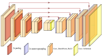
Figure 4: The customized U-Net used in our method, which maps the random noise input $\bm{z_{r}}$ to the residual $\bm{r}$.

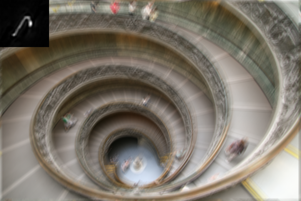
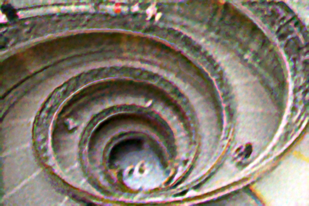
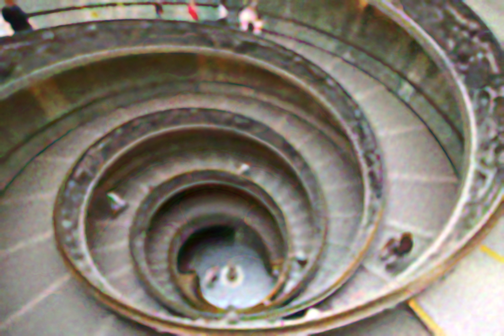
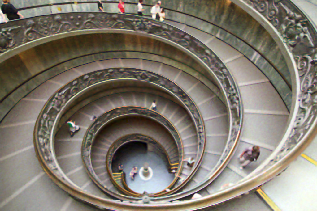
Blurry	PSNR 18.32	PSNR 21.82	PSNR 24.02
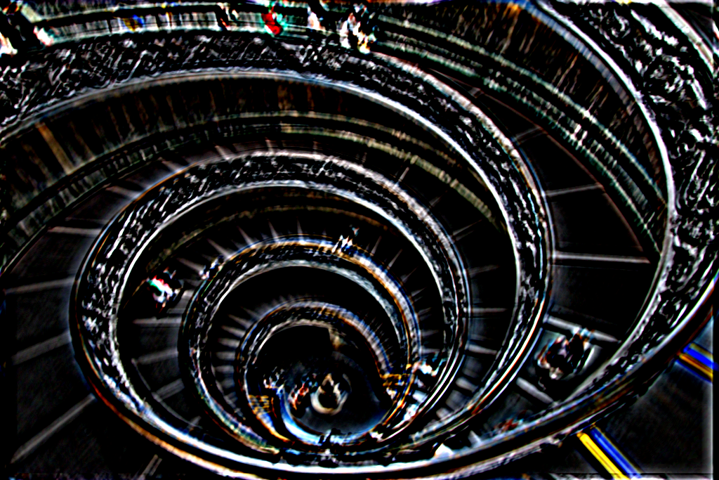
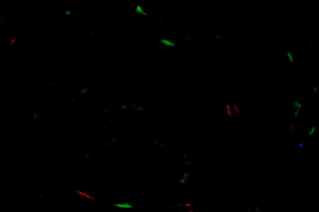
MSE 0	MSE 0.0274	MSE 0.0126	MSE 0.0046
True Res.	FCN	U-Net	Ours

Figure 5: The influence of different network architectures for DRP. Row 1: the deblurred results of the image in the dataset of [12]. Row 2: the estimated residuals. The input kernel for deblurring is estimated by the method in [3]. The closer estimated residual is to the true residual, the better it is.

We discuss the influence of different network architectures for DRP. Three network architectures are used for comparison: (i) fully connected network (FCN), (ii) U-Net, and (iii) the customized U-Net (see Figure 4), in which the soft-shrinkage is used to replace the sigmoid. Figure 5 displays the deblurred results and estimated residuals by using different network architectures. We can observe from the results that the customized U-Net is more favorable to capture the residual as compared to FCN and U-Net. The vanishing gradient issue is encountered for the sigmoid function when training neural networks for the residual with subtle values. Thus, the customized U-Net, which replaces the sigmoid function with the soft-shrinkage function, can better capture the residual as the soft-shrinkage can ameliorate this issue as compared to the sigmoid function. Consequently, we can observe from Figure 5 that a better estimation of the residual boosts the quality of image restoration.

4.3 Performance on Benchmark Datasets

We comprehensively compare our method with state-of-the-art methods on simulated data and real data. The simulated data comes from the datasets of Levin et al. [13] and Lai et al. [12], in which the Gaussian noise level is set to be 1%. The real data comes from the dataset of Lai et al. [12]. The dataset of Levin et al. [13] contains 32 blurry images that are blurred with 4 sharp images and 8 blur kernels. The dataset of Lai et al. [12] contains 102 real blurry images and 100 simulated blurry images that are blurred with 25 sharp images and 4 blur kernels.

Kernel Estimation. The estimated kernels for the dataset of Levin et al. [13] are obtained by applying five blind deblurring algorithms, including Cho et al. [2], SelfDeblur by Ren et al. [24], Levin et al. [13], Pan et al. [21], and Sun et al. [31]. The estimated kernels for the dataset of Lai et al. [12] are obtained by four blind deblurring methods, including Xu et al. [37], Xu et al. [16], Sun et al. [31], and Perrone et al. [3]. Note that, two groups of different kernel estimation algorithms are chosen for two datasets respectively to follow the settings in the compared methods.

MSE 0	MSE 0.012	MSE 0.003	MSE 0.026	MSE 0.002
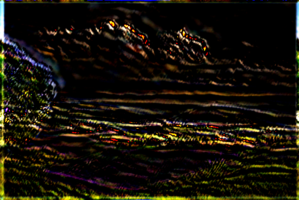
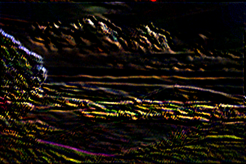
MSE 0	MSE 0.050	MSE 0.047	MSE 0.020	MSE 0.009
True Res.	Res. in [8]	Res. in [34]	Res. in [7]	Ours

Figure 6: The estimated residual by semi-blind methods on the images from datasets of Levin et al. [13] and Lai et al. [12]. The closer estimated residual is to the true residual, the better it is.

Table 2: Average PSNR/SSIM comparison of deblurred results by different methods on the dataset of Levin et al. [13] and Lai et al. [12] using different estimated kernels.

		BD	NBD			SBD
Datasets		Ren et al. [24]	Krishnan et al. [11]	Ren et al. [23]	Eboli et al. [6]	Zhao et al. [41]	Ji & Wang[8]	Vasu et al. [34]	Fang et al. [7]	Ours
Levin et al. [13]	Cho et al. [2]	28.52/0.80	28.12/0.82	28.49/0.81	28.54/0.82	28.76/0.82	28.55/0.83	29.50/0.84	29.86/0.85	30.52/0.88
	Levin et al. [14]		28.17/0.83	28.55/0.83	28.93/0.84	27.96/0.81	28.79/0.83	29.65/0.85	29.91/0.86	30.78/0.89
	Ren et al. [24]		27.88/0.82	27.59/0.80	27.74/0.82	27.19/0.80	27.39/0.82	29.01/0.85	28.57/0.83	29.55/0.86
	Pan et al. [21]		29.84/0.86	29.99/0.86	30.58/0.87	28.98/0.83	29.21/0.86	31.62/0.87	31.98/0.91	32.28/0.92
	Sun et al. [31]		29.30/0.85	29.91/0.86	30.90/0.87	28.99/0.83	29.10/0.86	30.75/0.88	31.05/0.89	31.84/0.91
	Average	28.52/0.80	28.66/0.83	28.91/0.83	29.34/0.84	28.38/0.82	28.61/0.84	30.10/0.86	30.27/0.87	31.01/0.89
Lai et al. [12]	Xu et al. [37]	17.69/0.64	17.73/0.65	17.61/0.56	19.53/0.64	19.60/0.64	19.67/0.61	20.21/0.67	20.67/0.68	21.07/0.68
	Xu et al. [16]		18.83/0.62	17.81/0.57	19.52/0.67	19.78/0.67	19.34/0.60	19.52/0.64	20.25/0.66	20.96/0.68
	Sun et al. [31]		17.96/0.61	17.99/0.57	20.04/0.69	19.83/0.69	20.10/0.68	19.88/0.67	20.44/0.68	21.03/0.70
	Perrone et al. [3]		17.57/0.63	16.88/0.54	18.89/0.62	19.56/0.65	19.21/0.60	19.12/0.60	19.87/0.62	20.31/0.64
	Average	17.69/0.64	18.02/0.63	17.57/0.56	19.49/0.66	19.69/0.66	19.58/0.63	19.68/0.65	20.31/0.66	20.84/0.68

Compared Methods. We select eight state-of-the-art methods as the baselines. These methods cover a blind deblurring (BD) method SelfDeblur [24] (in which the authors of [24] use the Levin et al.’s dataset and Lai et al.’s dataset without adding extra noise while the noise level in our setting is 1%), three non-blind (NBD) deblurring methods (i.e., Fergus et al. [28], Ren et al. [23], and Eboli et al. [6]), and four semi-blind deblurring (SBD) methods (i.e., Zhao et al. [41], Ji and Wang [8], Vasu et al. [34], Fang et al. [7]).

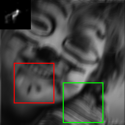
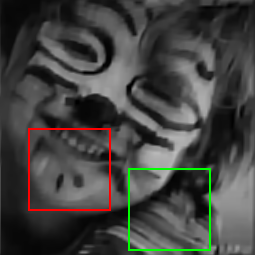
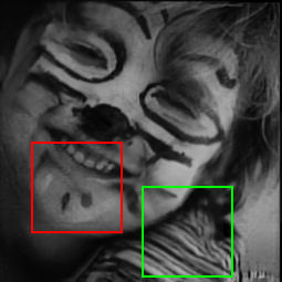
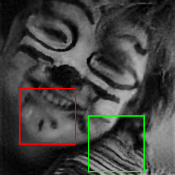
24.64/0.747	25.96/0.765	29.57/0.878	29.03/0.870	26.21/0.774	28.28/0.856	30.25/0.877	29.00/0.875	31.65/0.889
23.88/0.844	23.50/0.811	21.98/0.781	22.04/0.787	23.86/0.846	23.85/0.843	27.27/0.917	27.86/0.903	29.14/0.943
Blurry	[24]	[11]	[23]	[41]	[8]	[34]	[7]	Ours

Figure 7: The deblurred results by different methods on the images from the dataset of Levin et al. [13] with the kernel estimated by the method in [2] (row 1), and the dataset of Lai et al. [12] with the kernel estimated by the method in [3] (row 2). The numerical indexes at the bottom of each image indicate the PSNR/SSIM values. Zoom in for better visualization.

Tables 2 and 3 list the average PSNR/SSIM values of different methods on the datasets of Levin et al. [13] and Lai et al. [12]. From the tables, we can observe that the proposed method performs best on different blurs and images as compared with the competitive methods. Meanwhile, we observe that the blind method SelfDeblur [24] shows unpleasant performance. It is reasonable since SelfDeblur [24] does not handle the kernel uncertainty. The reason behind the failure of these non-blind methods, such as [11, 23, 6] should be that they are sensitive to the accuracy of estimated kernels. Among the SBD methods, the proposed method achieves the best quantitative results. The underlying reason is that the proposed method is empowered by a dataset-free DRP, which allows us to faithfully capture the residual as compared to hand-crafted priors [41, 8] and data-driven priors [34, 7].

Figure 6 and Figure 7 display the estimated residuals and restored results by different methods. From Figure 6, we observe that our method can preserve the fine details of residuals as compared to other methods. In Figure 7, it is not difficult to observe that the deblurred results by our method are much clearer and sharper than others. These observations validate the effectiveness of the proposed method. The visual quality is consistent with the improvement of quantitative performance gain.

Figure 8 displays the deblurred results of two real images from the dataset of Lai et al. [12] with the kernel estimated by the method in [21]. We can see that the BD method [24] does not deliver faithful deblurring results. NBD methods [11, 23] yield significant ringing artifacts in the restored images. Among the SBD methods, model-driven methods [41, 8] perform unpleasantly in deblurring while the data-driven methods [34, 7] slightly arouse outliers and artifacts. In comparison, our method, which leverages the power of the DRP, faithfully restores high-quality clear images and robustly handles the artifacts.

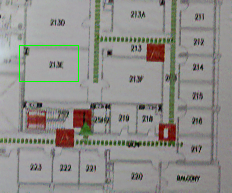
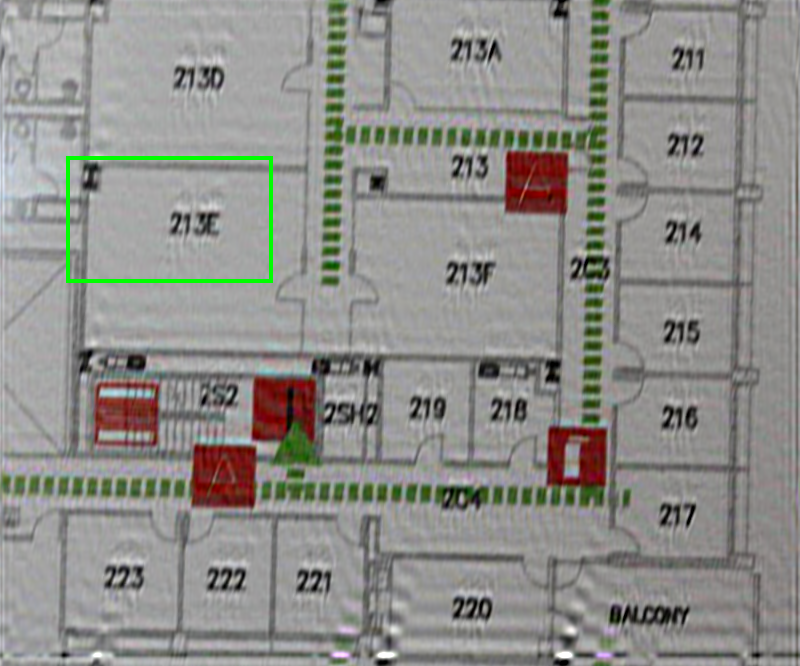
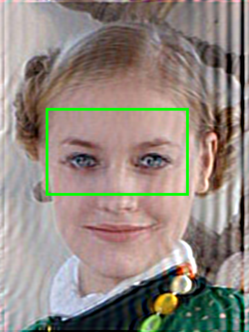
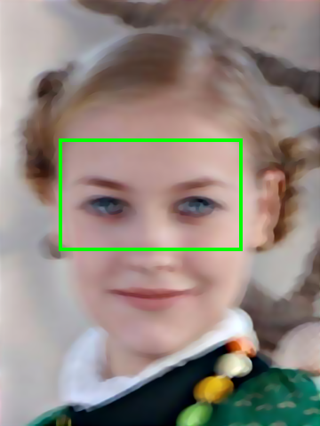
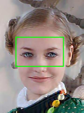
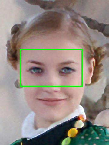
Blurry	[24]	[11]	[23]	[41]	[8]	[34]	[7]	Ours

Figure 8: The deblurred results by different methods on the real images from the dataset of Lai et al. [12] with the kernel estimated by the method in [21]. Zoom in for better visualization.

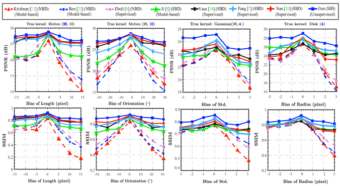
Figure 9: PSNR and SSIM values against bias of inaccurate kernel parameters obtained by different methods.

4.4 Robustness to Different Types of Kernel Error

In this section, we discuss the robustness of our method to different types of kernel error. Here we consider a motion blur with 20 pixels length and $10^{\circ}$ orientation, denoted by Motion $(20,10)$; a Gaussian blur with size $20\times 20$ and $\sigma=4$, denoted by Gaussian $(20,4)$; and a disk-like defocus blur with a radius of 4 pixels, denoted by Disk $(4)$. The test images are generated by blurring the sharp images (see supplementary materials) with the above kernels.

Inaccurate Kernel Setting. Different types of inaccurate kernels are generated by varying the parameters of different kernels, e.g., the variance in Gaussian, the orientation and length in Motion, and the radius in Disk.

Compared Methods. Five methods are selected as comparisons, including NBD [11, 23] and SBD [34, 8, 20] methods. In particular, the recent data-driven semi-blind method by Nan and Ji [20] is selected as a candidate since this method achieves soft-of-the-art performance and can efficiently estimate the residual on benchmark datasets in a supervised manner.

Figure 9 displays the PSNR and SSIM values against the bias of inaccurate kernel parameters. We can observe from the figure that the proposed method delivers pleasant robustness to kernel error and achieves the best quantitative performance in comparison with other methods. Besides, we can see that the NBD methods [11, 23] significantly deteriorate as the bias is amplified. The underlying reason is that they are sensitive to kernel error. As for other SBD methods, the model-driven method [8] is inferior to data-driven methods [34, 20] since the hand-crafted prior is generally insufficient in characterizing the complex residual. Data-driven based methods perform well in the case of motion blurs, but fail to continue their impressive performances in the cases of Gaussian and Disk blurs as they are vulnerable to out-of-distribution blurs and images. The reason for our success should be that we utilize the dataset-free DRP that is expressed by the untrained customized U-Net, which allows us to flexibly adapt to different blurs and images.

5 Conclusion

We proposed a dataset-free DRP for the residual induced by the kernel error depicted by a customized untrained deep neural network, which allowed us to generalize to different blurs and images in real scenarios. With the power of DRP, we then proposed an uncertainty-aware unsupervised image deblurring model incorporating deep priors and hand-crafted priors, in which all priors work together to deliver a promising performance. Extensive experiments on different blurs and images showed that the proposed method achieves notable performance as compared with the state-of-the-art methods in terms of image quality and the robustness to different types of kernel error.

References

- [1] Liang Chen, Jiawei Zhang, Jinshan Pan, Songnan Lin, Faming Fang, and Jimmy S Ren. Learning a non-blind deblurring network for night blurry images. In CVPR, pages 10542–10550, 2021.
- [2] Sunghyun Cho and Seungyong Lee. Fast motion deblurring. In ACM SIGGRAPH, pages 1–8. 2009.
- [3] Perrone Daniele and Favaro Paolo. Total variation blind deconvolution: The devil is in the details. In CVPR, pages 2909–2916, 2014.
- [4] Jiangxin Dong, Stefan Roth, and Bernt Schiele. Dwdn: Deep wiener deconvolution network for non-blind image deblurring. IEEE TPAMI, (01):1–1, 2021.
- [5] Weisheng Dong, Lei Zhang, Guangming Shi, and Xin Li. Nonlocally centralized sparse representation for image restoration. IEEE TIP, 22(4):1620–1630, 2013.
- [6] Thomas Eboli, Jian Sun, and Jean Ponce. End-to-end interpretable learning of non-blind image deblurring. In ECCV, 2020.
- [7] Yingying Fang, Hao Zhang, Hok Shing Wong, and Tieyong Zeng. A robust non-blind deblurring method using deep denoiser prior. In CVPRW, pages 735–744, June 2022.
- [8] Hui Ji and Kang Wang. Robust image deblurring with an inaccurate blur kernel. IEEE TIP, 21(4):1624–1634, 2011.
- [9] Jiaya Jia. Single image motion deblurring using transparency. In CVPR, pages 1–8, 2007.
- [10] Diederick P Kingma and Jimmy Ba. Adam: A method for stochastic optimization. In ICLR, 2015.
- [11] Dilip Krishnan and Rob Fergus. Fast image deconvolution using hyper-laplacian priors. NIPS, 22, 2009.
- [12] Wei-Sheng Lai, Jia-Bin Huang, Zhe Hu, Narendra Ahuja, and Ming-Hsuan Yang. A comparative study for single image blind deblurring. In CVPR, pages 1701–1709, 2016.
- [13] Anat Levin, Yair Weiss, Fredo Durand, and William T Freeman. Understanding and evaluating blind deconvolution algorithms. In CVPR, pages 1964–1971, 2009.
- [14] Anat Levin, Yair Weiss, Fredo Durand, and William T Freeman. Efficient marginal likelihood optimization in blind deconvolution. In CVPR, pages 2657–2664, 2011.
- [15] Ji Li, Yuesong Nan, and Hui Ji. Un-supervised learning for blind image deconvolution via monte-carlo sampling. Inverse Probl, 38(3):035012, 2022.
- [16] Xu Li, Zheng Shicheng, and Jia Jiaya. Unnatural sparse representation for natural image deblurring. In CVPR, pages 1107–1114, 2013.
- [17] Guangcan Liu, Shiyu Chang, and Yi Ma. Blind image deblurring using spectral properties of convolution operators. IEEE TIP, 23(12):5047–5056, 2014.
- [18] Jun Liu, Ming Yan, and Tieyong Zeng. Surface-aware blind image deblurring. IEEE TPAMI, 43(3):1041–1055, 2021.
- [19] Chong Mou, Qian Wang, and Jian Zhang. Deep generalized unfolding networks for image restoration. In Proceedings of the IEEE/CVF Conference on Computer Vision and Pattern Recognition, pages 17399–17410, 2022.
- [20] Yuesong Nan and Hui Ji. Deep learning for handling kernel/model uncertainty in image deconvolution. In CVPR, pages 2388–2397, 2020.
- [21] Jinshan Pan, Deqing Sun, Hanspeter Pfister, and Ming-Hsuan Yang. Blind image deblurring using dark channel prior. In CVPR, pages 1628–1636, 2016.
- [22] Yuhui Quan, Peikang Lin, Yong Xu, Yuesong Nan, and Hui Ji. Nonblind image deblurring via deep learning in complex field. 2021.
- [23] Dongwei Ren, Hongzhi Zhang, David Zhang, and Wangmeng Zuo. Fast total-variation based image restoration based on derivative alternated direction optimization methods. Neurocomputing, 170:201–212, 2015.
- [24] Dongwei Ren, Kai Zhang, Qilong Wang, Qinghua Hu, and Wangmeng Zuo. Neural blind deconvolution using deep priors. In CVPR, pages 3341–3350, 2020.
- [25] Dongwei Ren, Wangmeng Zuo, David Zhang, Jun Xu, and Lei Zhang. Partial deconvolution with inaccurate blur kernel. IEEE TIP, 27(1):511–524, 2017.
- [26] Dongwei Ren, Wangmeng Zuo, David Zhang, Lei Zhang, and Ming-Hsuan Yang. Simultaneous fidelity and regularization learning for image restoration. IEEE TPAMI, 43(1):284–299, 2019.
- [27] Wenqi Ren, Xiaochun Cao, Jinshan Pan, Xiaojie Guo, Wangmeng Zuo, and Ming-Hsuan Yang. Image deblurring via enhanced low-rank prior. IEEE TIP, 25(7):3426–3437, 2016.
- [28] Fergus Rob, Singh Barun, Hertzmann Aaron, Roweis Sam T, and Freeman William T. Removing camera shake from a single photograph. In ACM SIGGRAPH, pages 787–794. 2006.
- [29] Raúl Rojas. The Backpropagation Algorithm, pages 149–182. Springer Berlin Heidelberg, Berlin, Heidelberg, 1996.
- [30] Jian Sun, Wenfei Cao, Zongben Xu, and Jean Ponce. Learning a convolutional neural network for non-uniform motion blur removal. In CVPR, pages 769–777, 2015.
- [31] Libin Sun, Sunghyun Cho, Jue Wang, and James Hays. Edge-based blur kernel estimation using patch priors. In IEEE ICCP, pages 1–8, 2013.
- [32] Michaeli Tomer and Irani Michal. Blind deblurring using internal patch recurrence. In ECCV, pages 783–798, 2014.
- [33] Dmitry Ulyanov, Andrea Vedaldi, and Victor Lempitsky. Deep image prior. In CVPR, pages 9446–9454, 2018.
- [34] Subeesh Vasu, Venkatesh Reddy Maligireddy, and AN Rajagopalan. Non-blind deblurring: Handling kernel uncertainty with cnns. In CVPR, pages 3272–3281, 2018.
- [35] Yilun Wang, Junfeng Yang, Wotao Yin, and Yin Zhang. A new alternating minimization algorithm for total variation image reconstruction. SIAM J. Imaging Sci., 1(3):248–272, 2008.
- [36] Z Wang, X Cun, J Bao, W Zhou, J Liu, and H Uformer Li. A general u-shaped transformer for image restoration. In Proceedings of the IEEE/CVF Conference on Computer Vision and Pattern Recognition, New Orleans, LA, USA, pages 19–24, 2022.
- [37] Li Xu and Jiaya Jia. Two-phase kernel estimation for robust motion deblurring. In ECCV, pages 157–170, 2010.
- [38] Yanyang Yan, Wenqi Ren, Yuanfang Guo, Rui Wang, and Xiaochun Cao. Image deblurring via extreme channels prior. In CVPR, pages 4003–4011, 2017.
- [39] Syed Waqas Zamir, Aditya Arora, Salman Khan, Munawar Hayat, Fahad Shahbaz Khan, and Ming-Hsuan Yang. Restormer: Efficient transformer for high-resolution image restoration. In Proceedings of the IEEE/CVF Conference on Computer Vision and Pattern Recognition, pages 5728–5739, 2022.
- [40] Jiawei Zhang, Jinshan Pan, Wei-Sheng Lai, Rynson WH Lau, and Ming-Hsuan Yang. Learning fully convolutional networks for iterative non-blind deconvolution. In CVPR, pages 3817–3825, 2017.
- [41] Xile Zhao, Wei Wang, Tieyong Zeng, Tingzhu Huang, and Michael K. Ng. Total variation structured total least squares method for image restoration. SIAM J. Imaging Sci., 35, 2013.
- [42] Changyin Zhou, Stephen Lin, and Shree K Nayar. Coded aperture pairs for depth from defocus and defocus deblurring. IJCV, 93(1):53–72, 2011.
- [43] Wangmeng Zuo, Dongwei Ren, David Zhang, Shuhang Gu, and Lei Zhang. Learning iteration-wise generalized shrinkage–thresholding operators for blind deconvolution. IEEE TIP, 25(4):1751–1764, 2016.