Cosmological-model-independent determination of Hubble constant from fast radio bursts and Hubble parameter measurements

Abstract

We establish a cosmological-model-independent method to determine the Hubble constant $H_{0}$ from the localized fast radio bursts (FRBs) and the Hubble parameter measurements from cosmic chronometers and obtain a first such determination $H_{0}=71\pm 3~{}\mathrm{km/s/Mpc}$, with an uncertainty of 4%, from the eighteen localized FRBs and nineteen Hubble parameter measurements in the redshift range $0<z\leq 0.66$. This value, which is independent of the cosmological model, is consistent with the results from the nearby type Ia supernovae (SN Ia) data calibrated by Cepheids and the Planck cosmic microwave background radiation observations at the $1\sigma$ and 2$\sigma$ confidence level, respectively. Simulations show that the uncertainty of $H_{0}$ can be decreased to the level of that from the nearby SN Ia when mock data from 500 localized FRBs with 50 Hubble parameter measurements in the redshift range of $0<z\leq 1$ are used. Since localized FRBs are expected to be detected in large quantities, our method will be able to give a reliable and more precise determination of $H_{0}$ in the very near future, which will help us to figure out the possible origin of the Hubble constant disagreement.

1 introduction

The cosmological constant $\Lambda$ plus cold dark matter ($\Lambda$CDM) model is the simplest cosmological model which fits the observational data very well. Based on the $\Lambda$CDM model, the Planck Cosmic Microwave Background (CMB) radiation observations give a tight constraint on the Hubble constant $H_{0}$: $H_{0}=67.4\pm 0.5~{}\mathrm{km/s/Mpc}$ with an uncertainty about 0.7% (Planck Collaboration, 2020). This result however has a more than $5\sigma$ deviation from $H_{0}=73.04\pm 1.04~{}\mathrm{km/s/Mpc}$ with the uncertainty being about 1.42%, which is determined by the nearby type Ia supernovae (SN Ia) calibrated by Cepheids (Riess et al., 2022). Since these SN Ia, which are calibrated by using the distance ladder, are located in the very low-redshift region, $H_{0}$ determined with them can be regarded as almost cosmological-model-independent. The disagreement of $H_{0}$ between two different observations has became the most serious crisis in modern cosmology (Riess, 2020; Di Valentino et al., 2021; Perivolaropoulos et al., 2022; Dainotti et al., 2021, 2022), and it indicates that the assumed $\Lambda$CDM model used to determine the Hubble constant may be inconsistent with our present Universe or there may be potentially unknown systematic errors in the observational data. It is worth noting however that several studies have not found any systematics that could explain the discrepancy (Feeney et al., 2018; Efstathiou, 2014; Riess et al., 2016; Cardona et al., 2017; Zhang et al., 2017; Follin & Knox, 2018; Riess et al., 2018a, b). To precisely identify the possible origin of the $H_{0}$ disagreement, many other observational data are needed to constrain the Hubble constant. However, constraints from the vast majority of data usually depend on a pre-assumed cosmological model.

Undoubtedly, a cosmological-model-independent determination of the Hubble constant from observational data with a redshift region larger than that of the nearby SN Ia may shed light on the possible origin of the $H_{0}$ disagreement. In this letter, we propose a cosmological-model-independent method to determine the value of $H_{0}$ from the fast radio bursts (FRBs) and the Hubble parameter $H(z)$ measurements from cosmic chronometers, and present a first determination of $H_{0}$ with current such observational data that is independent of the cosmological model, i.e., $H_{0}$ ($H_{0}=71\pm 3~{}\mathrm{km/s/Mpc}$). Considering that a huge number of FRBs will be detected in the near future as more than one thousand FRB events are expected very day (Xiao et al., 2021), we expect to be able to achieve the precision of $H_{0}$ determination at the level from the nearby SN Ia with our method very soon.

FRBs are a type of frequently and mysteriously transient signals of millisecond duration with typical radiation frequency of $\sim$GHz (Lorimer et al., 2007; Petroff et al., 2019; Zhang, 2020, 2022; CHIME/FRB Collaboration, 2021). These signals are significantly dispersed by the ionized medium distributed along the path between the sources and the observer. The observed dispersion, quantified by the dispersion measure (DM), results mainly from the electromagnetic interaction between the signals and the free electrons in the intergalactic medium (IGM). Since the effects of the free electrons on the signals are cumulative with the increase of traveling distance of FRBs, the DM-redshift relations of FRBs can be used for cosmological purposes. For example, they have been used to determine the fraction of baryon mass in the IGM (Li et al., 2019; Lemos et al., 2022; Wei et al., 2019; Li et al., 2020), to constrain the cosmological parameters (Gao et al., 2014; Yang & Zhang, 2016; Walters et al., 2018), to explore the reionization history of our Universe (Caleb et al., 2019; Linder, 2020; Beniamini et al., 2021; Bhattacharya et al., 2021; Hashimoto et al., 2021; Lau et al., 2021; Pagano & Fronenberg, 2021; Heimersheim et al., 2022), to measure the Hubble parameter (Wu et al., 2020), to probe the interaction between dark energy and dark matter (Zhao et al., 2022a), and so on.

FRBs have also been used to determine the value of the Hubble constant (Li et al., 2018; Zhao et al., 2021; Hagstotz et al., 2022; James et al., 2022; Wu et al., 2022; Zhao et al., 2022b). Hagstotz et al. (2022) and Wu et al. (2022) have obtained constraints on $H_{0}$ of $62.3\pm 9.1~{}\mathrm{km/s/Mpc}$ and $68.81^{+4.99}_{-4.33}~{}\mathrm{km/s/Mpc}$ by utilizing nine and eighteen localized FRBs, respectively. Using sixteen localized FRBs and sixty unlocalized FRBs, James et al. (2022) have achieved $H_{0}=73^{-12}_{-8}~{}\mathrm{km/s/Mpc}$. These results rely unavoidably on an assumed cosmological model, usually $\Lambda$CDM, since the theoretical value of $\mathrm{DM}$ used in these studies is model-dependent. Interestingly, the derivative of $\mathrm{DM}$ with respect to the cosmic time $t$ is not dependent on any cosmological models although $\mathrm{DM}$ is, and moreover it is proportional to the Hubble constant squared. Therefore, the value of $H_{0}$ can be determined cosmological-model-independently if the time variation of $\mathrm{DM}$ can be observed directly. However, the time variation of $\mathrm{DM}$ due to the cosmic expansion is extremely weak, which is about $-5.6\times 10^{-8}(1+z)^{2}~{}\mathrm{pc/cm^{3}/yr}$ with $z$ being redshift (Yang & Zhang, 2017), and thus it is very difficult to measure directly. In this letter, we find a subtle way to avoid this problem so as to obtain $H_{0}$ cosmological-model-independently with FRBs, i.e., we propose to derive the time variation of $\mathrm{DM}$ through combining the redshift variation of $\mathrm{DM}$ of FRBs, which can be derived from the redshift distribution of FRBs, and the Hubble parameter measurements. Since the FRB and Hubble parameter data can be in the higher redshift region, our method contrasts with those using local measurements such as the Cepheid-calibrated SN Ia which can only be performed at very low redshifts.

2 Method

As is well-known, the radio pulse will be dispersed when it travels through the ionized IGM, which will result in different arrival times for photons with different frequencies. For two photons with the frequencies being $\nu_{1}$ and $\nu_{2}$ ($\nu_{1}<\nu_{2}$), respectively, the delayed arrival time can be expressed as

$$\Delta t=\frac{e^{2}}{2\pi m_{e}c}\left(\frac{1}{\nu_{1}^{2}}-\frac{1}{\nu_{2}^{2}}\right)\mathrm{DM}\,,$$ (1)

where $e$ and $m_{e}$ are the electron charge and mass, respectively, $c$ the speed of light, and DM is defined as

$$\mathrm{DM}\equiv\int\frac{n_{e,z}}{1+z}dl\,.$$ (2)

Here $dl$ is an infinitesimal proper length along the line of sight, and $n_{e,z}$ the number density of free electrons at redshift $z$. Therefore, DM carries the information of the distance and number density of free electrons. The observed DM is a combination of four different components:

$$\mathrm{DM_{obs}}=\mathrm{DM_{MW}^{ISM}}+\mathrm{DM_{MW}^{halo}}+\mathrm{DM_{IGM}}+\mathrm{DM_{host}}\ .$$ (3)

Here the subscript ‘$\mathrm{MW}$’, ‘$\mathrm{IGM}$’ and ‘$\mathrm{host}$’ represent the contributions from the Milky Way, the intergalactic medium and the host galaxy, respectively. The superscript ‘ISM’ and ‘halo’ denote the contributions from interstellar medium and halo of galaxy, respectively. Among them, $\mathrm{DM_{IGM}}$ depends on the cosmological model. However, since the IGM is inhomogeneous, we can only derive the average of $\mathrm{DM_{IGM}}$ theoretically (Deng & Zhang, 2014)

$$\langle\mathrm{DM_{IGM}}\rangle = \frac{3cH_{0}\Omega_{b0}}{8\pi Gm_{p}}\int_{0}^{z}\frac{f_{\mathrm{IGM}}(z)f_{e}(z)(1+z)}{E(z)}dz\,,$$ (4)

where $\Omega_{b0}$, $G$, $m_{p}$, and $f_{\mathrm{IGM}}(z)$ are the current baryon density parameter, the gravitational constant, the proton mass, and the fraction of baryon mass in the IGM, respectively, $E(z)=H(z)/H_{0}$ is the dimensionless Hubble parameter, which is given by the concrete cosmological model, and $f_{e}(z)=Y_{\mathrm{H}}f_{e,\mathrm{H}}(z)+\frac{1}{2}Y_{\mathrm{He}}f_{e,\mathrm{He}}(z)$ is the ratio of the number of free electrons to baryons in the IGM. Here $Y_{\mathrm{H}}\sim 3/4$ and $Y_{\mathrm{He}}\sim 1/4$ are the hydrogen (H) and helium (He) mass fractions, respectively, and $f_{e,\mathrm{H}}$ and $f_{e,\mathrm{He}}$ are the ionization fractions for H and He, respectively.

It is worth noting that $\langle\mathrm{DM_{IGM}}\rangle$ is evolving with the cosmic expansion. After applying the relation $dz=-H_{0}E(z)(1+z)dt$, we obtain the derivative of $\langle\mathrm{DM_{IGM}}\rangle$ with respect to the cosmic time $t$

$$\frac{d\langle\mathrm{DM_{IGM}}\rangle}{dt} = -\frac{3cH_{0}^{2}\Omega_{b0}}{8\pi Gm_{p}}f_{\mathrm{IGM}}(z)f_{e}(z)(1+z)^{2}\,,$$ (5)

which indicates that the variation of $\langle\mathrm{DM_{IGM}}\rangle$ with time is independent of the dimensionless Hubble parameter $E(z)$ and thus of any cosmological models. As a result, the value of the Hubble constant can be derived cosmological-model-independently from

$$H_{0} = \left[-\frac{8\pi Gm_{p}}{3c\Omega_{b0}f_{\mathrm{IGM}}(z)f_{e}(z)(1+z)^{2}}\frac{d\langle\mathrm{DM_{IGM}}\rangle}{dt}\right]^{\frac{1}{2}},$$ (6)

if one can obtain $d\langle\mathrm{DM_{IGM}}\rangle/dt$, and fix $\Omega_{b0}$, $f_{\mathrm{IGM}}(z)$ and $f_{e}(z)$. Since the variation of $\langle\mathrm{DM_{IGM}}\rangle$ from cosmic expansion is about $-5.6\times 10^{-8}(1+z)^{2}~{}\mathrm{pc/cm^{3}/yr}$ (Yang & Zhang, 2017), it is extremely weak and thus is very difficult to measure. Fortunately, $d\langle\mathrm{DM_{IGM}}\rangle/dt$ can be obtained as a product of $d\langle\mathrm{DM_{IGM}}\rangle/dz$ and $dz/dt$. The variation of $\langle\mathrm{DM_{IGM}}\rangle$ with time can be determined once both $d\langle\mathrm{DM_{IGM}}\rangle/dz$ and $dz/dt$ are known. The $dz/dt$ factor can be found directly from the Hubble parameter measurements from cosmic chronometers. If we work out the relation of $\langle\mathrm{DM_{IGM}}\rangle$ with $z$ from the observational data of FRBs, $d\langle\mathrm{DM_{IGM}}\rangle/dz$ at the redshifts of the Hubble parameter data points can be derived and then $d\langle\mathrm{DM_{IGM}}\rangle/dt$ at the same redshifts can be obtained. For example, employing a continuous piecewise linear function to approximate the $\langle\mathrm{DM_{IGM}}\rangle-z$ relation, we have

$$\langle\mathrm{DM_{IGM}}\rangle(z)=\frac{\langle\mathrm{DM_{IGM}}\rangle_{i+1}-\langle\mathrm{DM_{IGM}}\rangle_{i}}{z_{i+1}-z_{i}}\left(z-z_{i}\right)+\langle\mathrm{DM_{IGM}}\rangle_{i}\,,$$ (7)

after dividing uniformly the redshift range of FRB samples into $n$ bins with $n+1$ control points $z_{i}$. Here $\langle\mathrm{DM_{IGM}}\rangle_{i}$ is the undetermined dispersion measure at $z_{i}$, and $z_{1}=0$ is fixed. For the $n=1$ case, this function reduces to a linear function, and $z_{2}$ is the maximum redshift of FRB samples. Thus, we can fix $\langle\mathrm{DM_{IGM}}\rangle_{1}=0$, and obtain $\langle\mathrm{DM_{IGM}}\rangle_{2}$ from the observed $\langle\mathrm{DM_{IGM}}\rangle$ by using the Markov Chain Monte Carlo (MCMC) method. Taking the derivative of Eq. (7) with respect to $z$ yields the $d\langle\mathrm{DM_{IGM}}\rangle/dz-z$ relation, from which the values of $d\langle\mathrm{DM_{IGM}}\rangle/dt$ at the redshifts of the Hubble parameter measurements can be obtained after using the $H(z)$ data. Therefore, using Eq. (6), we can constrain the Hubble constant.

3 Data and results

We will use the latest localized FRBs data and the $H(z)$ data to determine $d\langle\mathrm{DM_{IGM}}\rangle/dt$. Our FRB samples are compiled in (Wu et al., 2022), which contain eighteen FRBs within the redshift range of $z\in(0,0.66]$ (Chatterjee et al., 2017; Bannister et al., 2019; Prochaska et al., 2019a; Ravi et al., 2019; Bhandari et al., 2020; Heintz et al., 2020; Law et al., 2020; Marcote et al., 2020; Bhardwaj et al., 2021; Chittidi et al., 2021; Bhandari et al., 2022). The number of the latest $H(z)$ data is 32, spanning redshifts from 0.07 to 1.965 (Simon et al., 2005; Stern et al., 2010; Moresco et al., 2012; Cong et al., 2014; Moresco, 2015; Moresco et al., 2016; Ratsimbazafy et al., 2017; Borghi et al., 2022), which are measured by using the cosmic chronometric technique (Jimenez & Loeb, 2002). Here we select only nineteen $H(z)$ data that fall in the redshift range of the FRB samples.

Since DM_obs is released for the FRB data, we use Eq. (3) to extract the extragalactic DM by deducting the contribution from the Milky Way in $\mathrm{DM_{obs}}$:

$$\mathrm{DM_{ext}^{obs}}=\mathrm{DM_{obs}}-\mathrm{DM_{MW}^{ISM}}-\mathrm{DM_{MW}^{halo}}-\Delta\mathrm{DM_{IGM}},$$ (8)

where $\Delta\mathrm{DM_{IGM}}$ represents the contribution of fluctuations of the electron density in the IGM, which is assumed to obey a normal distribution $\mathcal{N}(0,\sigma_{\mathrm{\Delta DM_{IGM}}})$ since the fluctuations in the electron density along the line of sight can be approximated by a Gaussian distribution (Jaroszynski, 2019; Macquart et al., 2020; Zhang et al., 2021). The $\mathrm{DM_{MW}^{ISM}}$ can be obtained from the current electron-density model of the Milky Way (Yao et al., 2017), and $\mathrm{DM_{MW}^{halo}}$ is assumed as $65~{}\mathrm{pc/cm^{3}}$ (Prochaska & Zheng, 2019b). Then the uncertainty $\sigma_{\mathrm{DM_{ext}}}$ of $\mathrm{DM_{ext}^{obs}}$ has the form

$$\sigma_{\mathrm{DM_{ext}}}^{2}=\sigma_{\mathrm{DM_{obs}}}^{2}+\sigma_{\mathrm{DM_{MW}}}^{2}+\sigma_{\mathrm{\Delta DM_{IGM}}}^{2}.$$ (9)

Here $\sigma_{\mathrm{DM_{obs}}}$ is given by the observation, $\sigma_{\mathrm{\Delta DM_{IGM}}}$ is the uncertainty of $\Delta\mathrm{DM_{IGM}}$, which is estimated through the approximation $\sigma_{\mathrm{\Delta DM_{IGM}}}/\langle\mathrm{DM_{IGM}}\rangle=20\%/\sqrt{z}$ given in (Kumar & Linder, 2019), and the uncertainty of $\mathrm{DM_{MW}}$ (containing the uncertainties of ISM and halo) is taken to be $54~{}\mathrm{pc/cm^{3}}$ (Heimersheim et al., 2022). Apparently, the theoretical value of $\mathrm{DM_{ext}}$ can be expressed as

$$\mathrm{DM_{ext}^{th}}=\langle\mathrm{DM_{IGM}}\rangle+\mathrm{DM_{host}}\ .$$ (10)

However, the contribution of the host galaxy ($\mathrm{DM_{host}}$) in Eq. (10) is not easy to determine since we do not know it very well. Here, we follow (Macquart et al., 2020; Zhang et al., 2020) to consider a prior log-normal distribution of $\mathrm{DM_{host}}$

$$P_{\mathrm{host}}(\mathrm{DM_{host}})=\frac{1}{\sqrt{2\pi\sigma^{2}}\mathrm{DM_{host}}}\exp\left[-\frac{(\ln\mathrm{DM_{host}}-\mu)}{2\sigma^{2}}\right].$$ (11)

For this log-normal distribution, the median and variance of $\mathrm{DM_{host}}$ are $e^{\mu}$ and $e^{2\mu+\sigma^{2}}(e^{\sigma^{2}}-1)$, respectively. In (Zhang et al., 2020), the value of the median $e^{\mu}$ is assumed to be redshift-evolutionary: $e^{\mu}\equiv A(1+z)^{\alpha}$ with $A$ and $\alpha$ being two constants. Once the allowed regions of $A$ and $\alpha$ are determined from $\mathrm{DM_{ext}^{obs}}$, their best fitting values and uncertainties give the median and variation of $\mathrm{DM_{host}}$, respectively. Before running the MCMC to constrain all free parameters, we need to set the prior regions of $A$ and $\alpha$, which are obtained by using the IllustrisTNG simulation (Zhang et al., 2020). Moreover, as what was done in (Zhang et al., 2020), we place the host galaxies of FRBs into three types: (I) The repeating FRBs in a dwarf galaxy like the FRB 121102, (II) the repeating FRBs in a spiral galaxy like the FRB 180916, and (III) the non-repeating FRBs. Thus, we set $\left\{A_{1},\;\alpha_{1},\;A_{2},\;\alpha_{2},\;A_{3},\;\alpha_{3}\right\}$ as free parameters to describe the values of FRB’ $\mathrm{DM_{host}}$ in Eq. (10). These six parameters will be fitted simultaneously with the coefficients in Eq. (7), and are marginalized in the subsequent analysis.

For the piecewise linear function with $n=1$, we obtain $\langle\mathrm{DM_{IGM}}\rangle_{2}=641^{+144}_{-154}~{}\mathrm{pc/cm^{3}}$ from the eighteen FRB data points. Figure 1 shows the approximate $\langle\mathrm{DM_{IGM}}\rangle-z$ relation. Combining nineteen Hubble parameter data with the values of $d\langle\mathrm{DM_{IGM}}\rangle/dz$ at the redshifts of the $H(z)$ data, we obtain nineteen $d\langle\mathrm{DM_{IGM}}\rangle/dt$ data points. To further calculate the value of $H_{0}$, we fix $\Omega_{b0}=0.0487\pm 0.0005$ (DES Collaboration, 2022). Due to the lack of evidence for the evolution of $f_{\mathrm{IGM}}$ over the redshift range covered by the FRB sample, we adopt, in our analysis, $f_{\mathrm{IGM}}(z)=0.84^{+0.16}_{-0.22}$, which is determined by a cosmological-insensitive method (Li et al., 2020). Since the H and He are fully ionized at $z<3$ (Meiksin, 2009; Becker et al., 2011), i.e., $f_{e,\mathrm{H}}=f_{e,\mathrm{He}}=1$, we set $f_{e}(z)=7/8$ in our analysis. Finally, nineteen $H_{0}$ are derived from Eq. (6). Using the minimum $\chi^{2}$ method, we arrive at a constraint on $H_{0}$: $H_{0}=71\pm 3~{}\mathrm{km/s/Mpc}$ with an uncertainty of 4%. Figure 2 shows a comparison between our result with those obtained by the Planck CMB observations (Planck Collaboration, 2020) and the nearby SN Ia data (Riess et al., 2022). Our result is consistent with that from nearby SN Ia at the 1$\sigma$ confidence level (CL), but that from the CMB observations only at the $2\sigma$ CL.

Since $\Omega_{b0}=0.0487\pm 0.0005$ (DES Collaboration, 2022), which is used in above analysis, depends on the $\Lambda$CDM model, to study the effect of this model-dependent value on our result, we also consider $\Omega_{b0}=0.048\pm 0.001$ from the $w$CDM model (DES Collaboration, 2022), and obtain $H_{0}=71\pm 3~{}\mathrm{km/s/Mpc}$. This result is consistent very well with that in the case of $\Omega_{b0}=0.0487\pm 0.0005$. To further investigate the effect of the uncertainty of $\Omega_{b0}$ on our result, we choose a value of $\Omega_{b0}$ with a larger uncertainty: $\Omega_{b0}=0.0487\pm 0.02$, and achieve $H_{0}=71\pm 5~{}\mathrm{km/s/Mpc}$ with $7$% uncertainty. Apparently, when the uncertainty of $\Omega_{b0}$ increases 40 times (from $0.0005$ to $0.02$), the uncertainty of $H_{0}$ only increases $3\%$, which indicates that the precision of $H_{0}$ does not depend sensitively on the uncertainty of $\Omega_{b0}$. Thus, we conclude that the value of $H_{0}$ from our method is insensitive to $\Omega_{b0}$.

Let us now examine whether the adoption of the $n=1$ piecewise linear function leads to some bias in our results. For this purpose, we perform a further analyis by using the $n=2$ piecewise linear function and the quadratic polynomial function ($\langle\mathrm{DM_{IGM}}\rangle(z)=Az+Bz^{2}$) to approximate the $\langle\mathrm{DM_{IGM}}\rangle-z$ relation, where A and B are two constants. The constraints on the Hubble constant are $H_{0}=71\pm 5~{}\mathrm{km/s/Mpc}$ and $H_{0}=71\pm 4~{}\mathrm{km/s/Mpc}$ for the $n=2$ piecewise linear function and the quadratic polynomial, respectively. Apparently, the constraints on $H_{0}$ are very well consistent with each other for three different approximations. Thus, we can conclude that the $H_{0}$ results are almost independent of the functions chosen to approximate the redshift evolution of $\langle\mathrm{DM_{IGM}}\rangle(z)$.

Let us note that our results are slightly tighter than $H_{0}=75.7^{+4.5}_{-4.4}~{}\mathrm{km/s/Mpc}$ obtained model-independently from four strong gravitational lensing systems and SN Ia (Collett et al., 2019), which is later improved to $H_{0}=72.8^{+1.6}_{-1.7}~{}\mathrm{km/s/Mpc}$ when six strong gravitational lensing systems are used (Liao et al., 2020). These cosmological-model-independent results from strong lensing systems and SN Ia are consistent with $72.5^{+2.1}_{-2.3}~{}\mathrm{km/s/Mpc}$ (Birrer et al., 2019) and $73.3^{+1.7}_{-1.8}~{}\mathrm{km/s/Mpc}$ (Wong et al., 2020) obtained before from the four and six lensing systems respectively with an assumed spatially flat $\Lambda$CDM model. Furthermore, simulations show that 400 lensing systems can constrain $H_{0}$ model-independently with an uncertainty at the level of the nearby SN Ia (Collett et al., 2019).

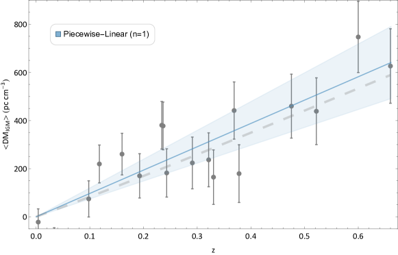
Figure 1: The $\langle\mathrm{DM_{IGM}}\rangle-z$ relation for the $n=1$ piecewise linear function (blue line). The shadow region denotes the 1$\sigma$ uncertainty. The gray points are eighteen $\langle\mathrm{DM_{IGM}}\rangle$ data samples. The dashed line is the theoretical value of $\langle\mathrm{DM_{IGM}}\rangle$ based on the $\Lambda$CDM model.

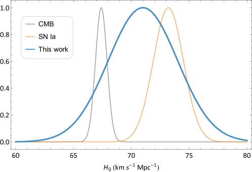
Figure 2: The constraints on $H_{0}$. The gray and orange lines represent the results from the Planck CMB observations and the nearby SN Ia data, respectively. The blue line shows our result.

To see how many FRBs are needed for a determination $H_{0}$ as precise as of the level of the nearby SN Ia, we need to use the Monte Carlo simulation. During simulation, we choose the spatially flat $\Lambda$CDM model with $H_{0}=73.04~{}\mathrm{km/s/Mpc}$ and $\Omega_{\mathrm{m0}}=0.3$ to be the fiducial model and set $\Omega_{b0}=0.0487$, $f_{\mathrm{IGM}}=0.84$, and $f_{e}(z)=7/8$. Here we randomly sample $\mathrm{DM_{ext}^{sim}}$ as the observed quantity, which is obtained from $\mathrm{DM_{IGM}^{sim}}+\mathrm{DM_{host}^{sim}}$. The redshift distribution of FRBs is assumed to be $P(z)\propto z^{2}\exp(-7z)$ in the redshift range $0<z\leq 1$ (Hagstotz et al., 2022). At the mock redshift $z$, the fiducial value of $\langle\mathrm{DM_{IGM}^{fid}}\rangle$ can be calculated from Eq. (4). The $\mathrm{DM_{IGM}^{sim}}$ is sampled from $\mathcal{N}\left(\langle\mathrm{DM_{IGM}^{fid}}\rangle,\sigma_{\mathrm{\Delta DM_{IGM}}}\right)$ with $\sigma_{\mathrm{\Delta DM_{IGM}}}=20\%\langle\mathrm{DM_{IGM}^{fid}}\rangle/\sqrt{z}$ (Kumar & Linder, 2019). $\mathrm{DM_{host}^{sim}}$ is simulated by using the distribution $P_{\mathrm{host}}(\mathrm{DM_{host}})$ given in Eq. (11). The type of the host galaxy is chosen randomly as one of the three different types, and the prior values of the parameters $\mu$ and $\sigma$ are set from the IllustrisTNG simulation (Zhang et al., 2020). Meanwhile, we also sample the $H(z)$ data with a uniform distribution at $0<z\leq 1$ following (Ma & Zhang, 2011). We simulate 500 FRBs and 50 $H(z)$ data. The larger number of data set prompts us to use the piecewise linear function with $n=2$ to approximate $\langle\mathrm{DM_{IGM}}\rangle-z$ relation. To minimize randomness and to ensure that the final constraint result is unbiased, we repeat the above steps 100 times and finally obtain $H_{0}=73.7\pm 1.4~{}\mathrm{km/s/Mpc}$. This indicates that the uncertainty of $H_{0}$ can be decreased to 1.9% from mock data, which is almost of the same precision as that from the nearby SN Ia (1.42%).

A high precision determination of $H_{0}$ from FRBs is expected soon since a large number of localized FRBs will be detected in the next few years. This is because there are huge number of FRB events every day and the detection ability is being improved rapidly. The running and upcoming radio telescopes and surveys include the Swinburne University of Technology’s digital backend for the Molonglo Observatory Synthesis Telescope array (UTMOST) (Caleb et al., 2016), the Canadian Hydrogen Intensity Mapping Experiment (CHIME) (CHIME/FRB Collaboration, 2021; Bandura et al., 2014), the Hydrogen Intensity and Real-time Analysis eXperiment (HIRAX) (Newburgh et al., 2016), the Five-hundred-meter Aperture Spherical Telescope (FAST) (Li et al., 2018), and the Square Kilometre Array (SKA) project (Macquart et al., 2015; Fialkov & Loeb, 2017).

4 Conclusion

The disagreement between the measurements of the Hubble constant from the CMB observations and the nearby SN Ia data has became one of the pressing challenges in modern cosmology. A cosmological-model-independent method to determine the value of $H_{0}$ from the data in the redshift region larger than that of the nearby SN Ia may serve as a probe to the possible origin of $H_{0}$ disagreement. In this letter, we establish a feasible way to cosmological-model-independently constrain $H_{0}$ by combining the variation of $\langle\mathrm{DM_{IGM}}\rangle$ with the redshift of FRBs and the Hubble parameter measurements, and obtain a first such determination $H_{0}=71\pm 3~{}\mathrm{km/s/Mpc}$ with data from the eighteen localized FRBs and nineteen Hubble parameter measurements in the redshift range $0<z\leq 0.66$. Remarkably, this value, which is independent of the cosmological model, lies in the middle of the results from CMB observations and the nearby SN Ia data, and it is consistent with those from the nearby SN Ia data and the CMB observations at the $1\sigma$ and $2\sigma$ CL, respectively. The uncertainty of our result is much less than what were obtained from FRBs in the framework of $\Lambda$CDM model (Hagstotz et al., 2022; Wu et al., 2022; James et al., 2022).

However, as our result has large uncertainty, it does not show significant statistic evidence for preferring the result from the nearby SN Ia data. Through the Monte Carlo simulation, we further investigate how many FRBs and $H(z)$ measurements are needed to more precisely determine the value of $H_{0}$. We find that the uncertainty of $H_{0}$ from mock 500 localized FRBs and 50 $H(z)$ data at $0<z\leq 1$ can be decreased to $1.9\%$, which is of the same level as that from the nearby SN Ia data. Since localized FRBs are expected to be detected in large quantities, the method established in this paper will be able to give a reliable and more precise determination of $H_{0}$ in the very near future, which will help us to figure out the possible origin of the Hubble constant disagreement.

References

- Bandura et al. (2014) Bandura, k., Addison, G. E., Amiri, M., et al. 2014, Ground-Based Airborne Telesc. V, 9145, 914522
- Bannister et al. (2019) Bannister, K. W., Deller, A. T., Phillips, C., et al. 2019, Science , 365, 565
- Becker et al. (2011) Becker, G. D., Bolton, J. S., Haehnelt, M. G., & Sargent, W. L. W. 2011, MNRAS, 410, 1096
- Beniamini et al. (2021) Beniamini, P., Kumar, P., Ma, X., & Quataert, E. 2021, MNRAS, 502, 5134
- Bhandari et al. (2020) Bhandari, S., Sadler, E. M., Prochaska, J. X., et al. 2020, ApJL, 895, L37
- Bhandari et al. (2022) Bhandari, S., Heintz, K, E., Aggarwal, K., et al. 2022, AJ, 163, 69
- Bhardwaj et al. (2021) Bhardwaj, M., Kirichenko, A. Y., Michilli, D., et al. 2021, ApJL, 919, L24
- Bhattacharya et al. (2021) Bhattacharya, M., Kumar, P., & Linder, E. V. 2021, Phys. Rev. D, 103, 103526
- Birrer et al. (2019) Birrer, S., Treu, T., Rusu, C. E., et al. 2019, MNRAS, 484, 4726
- Borghi et al. (2022) Borghi, N., Moresco, M., & Cimatti, A. 2022, ApJ, 928, L4
- Caleb et al. (2016) Caleb, M., Flynn, C., Bailes, M., et al. 2016, MNRAS, 458, 718
- Caleb et al. (2019) Caleb, M., Flynn, C., & Stappers, B. W. 2019, MNRAS, 485, 2281
- Cardona et al. (2017) Cardona, W., Kunz, M., & Pettorino, V. 2017, J. Cosmology Astropart. Phys, 03, 056
- Chatterjee et al. (2017) Chatterjee, S., Law, C. J., Wharton, R. S. et al. 2017, Nature, 541, 58
- CHIME/FRB Collaboration (2021) CHIME/FRB Collaboration, 2021, ApJS, 257, 59
- Chittidi et al. (2021) Chittidi, J, S., Simha, S., Mannings, A., et al. 2021, ApJ, 922, 173
- Collett et al. (2019) Collett, T., Montanari, F., & Räsänen, S. 2019, PhRvL, 123, 231101
- Cong et al. (2014) Cong, Z., Han, Z., Shuo, Y., et al. 2014, RAA, 14, 1221
- Dainotti et al. (2021) Dainotti, M. G., Simone, B. D., Schiavone, T., et al. 2021, ApJ, 912, 150
- Dainotti et al. (2022) Dainotti, M. G., Simone, B. D., Schiavone, T., et al. arXiv: 2201.09848
- DES Collaboration (2022) DES Collaboration, 2022, Phys. Rev. D, 105, 023520
- Deng & Zhang (2014) Deng, W., & Zhang, B. 2014, ApJ, 783, L35
- Di Valentino et al. (2021) Di Valentino, E., Mena, O., Pan, S., et al. 2021, CQGra, 38, 153001
- Efstathiou (2014) Efstathiou, G. 2014, MNRAS, 400, 1138
- Feeney et al. (2018) Feeney, S. M., Mortlock, D. J, & Dalmasso, N. 2018, MNRAS, 476, 3861
- Fialkov & Loeb (2017) Fialkov, A., & Loeb, A., 2017, ApJ, 846, L27
- Follin & Knox (2018) Follin, B., & Knox, L. 2018, MNRAS, 477, 4534
- Gao et al. (2014) Gao, H., Li, Z., & Zhang, B. 2014, ApJ, 788, 189
- Hagstotz et al. (2022) Hagstotz, S., Reischke, R., & Lilow, R. 2022, MNRAS, 511, 662
- Hashimoto et al. (2021) Hashimoto, T., Goto, T., Lu, T.-Y., et al. 2021, MNRAS, 502, 2346
- Heimersheim et al. (2022) Heimersheim, S., Sartorio, N. S., Fialkov, A., & Lorimer, D. R. 2022, ApJ, 933, 57
- Heintz et al. (2020) Heintz, K, E., Prochaska, J, X., Simha, S., et al. 2020, ApJ, 903, 152
- James et al. (2022) James, C. W., Ghosh, E M, Prochaska, J X., et al. 2022, MNRAS, 516, 4862
- Jaroszynski (2019) Jaroszynski, M. 2019, MNRAS, 484, 1637
- Jimenez & Loeb (2002) Jimenez, R., & Loeb, A. 2002, ApJ, 573, 37
- Kumar & Linder (2019) Kumar, P., & Linder, E. V. 2019, PhRvD, 100, 083533
- Lau et al. (2021) Lau, A. W. K., Mitra, A., Shafiee, M., & Smoot, G. 2021, NewA, 89, 101627
- Law et al. (2020) Law, C, J., Butler, B, J., Prochaska, J, X., et al. 2020, ApJ, 899, 161
- Lemos et al. (2022) Lemos, T., Gonçalves, R. S., Carvalho, J. C., & Alcaniz, J. S. 2022, arXiv:2205.07926
- Li et al. (2018) Li, D., Wang, P., Qian, L., et al. 2018, IEEE Microwave Magazine, 19, 112
- Li et al. (2018) Li, Z.-X., Gao, H., Ding, X.-H., Wang, G.-J., & Zhang, B. 2018, Nat Commun, 9, 3833
- Li et al. (2019) Li, Z., Gao, H., Wei, J.-J., et al. 2019, ApJ, 876, 146
- Li et al. (2020) Li, Z., Gao, H., Wei, J.-J., et al. 2020, MNRAS Lett., 496, L28
- Liao et al. (2020) Liao, K., Shafieloo, A., Keeley, R. E., & Linder, E. V. 2020, ApJL, 895, L29
- Linder (2020) Linder, E. V. 2020, Phys. Rev. D, 101, 103019
- Lorimer et al. (2007) Lorimer, D. R., Bailes, M., McLaughlin, M. A., Narkevic, D. J., & Crawford, F. 2007, Science, 318, 777
- Ma & Zhang (2011) Ma, C., & Zhang, T-J. 2011, ApJ, 730, 74
- Macquart et al. (2015) Macquart, J.-P., Keane, E., Grainge, K., et al. 2015, arXiv:1501.07535
- Macquart et al. (2020) Macquart, J. P., Prochaska, J. X., McQuinn, M., et al. 2020, Nature, 581, 391
- Marcote et al. (2020) Marcote, B., Nimmo, K., Hessels, J. W. T., et al. 2020, Nature, 577, 190
- Meiksin (2009) Meiksin, A. A. 2009, RvMP, 81, 1405
- Moresco et al. (2012) Moresco, M., Cimatti, A., Jimenez, R., et al. 2012, J. Cosmology Astropart. Phys, 08, 006
- Moresco (2015) Moresco, M. 2015, MNRAS Lett., 450, L16
- Moresco et al. (2016) Moresco, M., Pozzetti, L., Cimatti, A. et al. 2016, J. Cosmology Astropart. Phys, 05, 014
- Newburgh et al. (2016) Newburgh, L. B., Bandura, K., Bucher, M. A., et al. 2016, Ground-Based Airborne Telesc. VI, 9906, 99065X
- Pagano & Fronenberg (2021) Pagano, M., & Fronenberg, H. 2021, MNRAS, 505, 2195
- Perivolaropoulos et al. (2022) Perivolaropoulos, L., & Skara, F., 2022, New Astron. Rev., 95, 101659
- Petroff et al. (2019) Petroff, E., Hessels, J. W. T., & Lorimer, D.R. 2019, Astron Astrophys Rev, 27, 4
- Planck Collaboration (2020) Planck Collaboration, 2020, A&A, 641, A6
- Prochaska et al. (2019a) Prochaska, J, X., Macquart, J.-P., Mcquinn, M., et al. 2019a, Science , 366, 231
- Prochaska & Zheng (2019b) Prochaska J. X., & Zheng Y. 2019b, MNRAS, 485, 648
- Ratsimbazafy et al. (2017) Ratsimbazafy, A. L., Loubser, S. I., Crawford, S. M., et al. 2017, MNRAS, 467, 3239
- Ravi et al. (2019) Ravi, V., Catha, M., D′Addario, L., et al. 2019, Nature, 572, 352
- Riess et al. (2016) Riess, A. G., Macri, L. M., Hoffmann, S. L., et al. 2016, ApJ, 826, 56
- Riess et al. (2018a) Riess, A. G., Casertano, S., Yuan, W., et al. 2018a, ApJ, 855, 136
- Riess et al. (2018b) Riess, A. G., Casertano, S., Yuan, W., et al. 2018b, ApJ, 861, 126
- Riess (2020)
- Riess (2020) Riess A. G. 2020, Nature Rev. Phys., 2, 10
- Riess et al. (2022) Riess, A. G., Yuan, W., Macri, L. M., et al. 2022, ApJ, 934, L7
- Simon et al. (2005) Simon J., Verde L., & Jimenez R. 2005, Phys. Rev. D, 71, 123001
- Stern et al. (2010) Stern, D., Jimenez, R., Verde, L., Kamionkowski, M., & Stanford, S. A. 2010, J. Cosmology Astropart. Phys, 02, 008
- Walters et al. (2018) Walters, A., Weltman, A., Gaensler, B. M., Ma, Y.-Z., & Witzemann, A. 2018, ApJ, 856, 65
- Wei et al. (2019) Wei, J.-J., Li, Z., Gao, H., & Wu, X.-F. 2019, J. Cosmology Astropart. Phys, 09, 039
- Wong et al. (2020) Wong, K. C., Suyu, S. H., Chen, G. C-F., et al. 2020, MNRAS, 498, 1420
- Wu et al. (2020) Wu, Q., Yu, H., & Wang, F. Y. 2020, ApJ, 895, 33
- Wu et al. (2022) Wu, Q., Zhang, G-Q., & Wang, F. Y. 2022, MNRAS Lett., 515, L1
- Xiao et al. (2021) Xiao, D., Wang, F., & Dai, Z. 2021, Sci. China Phys. Mech. Astron., 64, 249501
- Yang & Zhang (2016) Yang, Y.-P., & Zhang, B. 2016, ApJ, 830, L31
- Yang & Zhang (2017) Yang, Y.-P., & Zhang, B. 2017, ApJ, 847, 22
- Yao et al. (2017) Yao J. M., Manchester R. N., Wang N. 2017, ApJ, 835, 29
- Zhang (2020) Zhang, B. 2020, Nature, 587, 45
- Zhang (2022) Zhang, B. 2022, arXiv:2212.03972
- Zhang et al. (2017) Zhang, B. R., Childress, M. J., Davis, T. M., et al. 2017, MNRAS, 471, 2254
- Zhang et al. (2020) Zhang, G. Q., Yu, H., He, J. H., & Wang, F. Y. 2020, ApJ, 900, 170
- Zhang et al. (2021) Zhang, Z. J., Yan, K., Li, C. M., Zhang, G. Q.,& Wang, F. Y. 2021, ApJ, 906, 49
- Zhao et al. (2021) Zhao, S., Liu, B., Li, Z., & Gao, H. 2021, ApJ, 916, 70
- Zhao et al. (2022a) Zhao, Z-W., Wang, L-F., Zhang, J-G., Zhang, J-F., & Zhang, X. 2022, arXiv:2210.07162
- Zhao et al. (2022b) Zhao, Z-W., Zhang, J-G., Li, Y., et al. 2022, arXiv:2212.13433