Primordial non-Guassianity in inflation with gravitationally enhanced friction

Abstract

The gravitationally enhanced friction can reduce the speed of the inflaton to realize an ultra-slow-roll inflation, which will amplify the curvature perturbations. The amplified perturbations can generate a sizable amount of primordial black holes (PBHs) and induce simultaneously a significant background gravitational waves (SIGWs). In this paper, we investigate the primordial non-Gaussianity of the curvature perturbations in the inflation with gravitationally enhanced friction. We find that when the gravitationally enhanced friction plays a role in the inflationary dynamics, the non-Gaussianity is noticeably larger than that from the standard slow-roll inflation. During the regime in which the power spectrum of the curvature perturbations is around its peak, the non-Gaussianity parameter changes from negative to positive. When the power spectrum is at its maximum, the non-Gaussianity parameter is near zero ($\sim\mathcal{O}(0.01)$). Furthermore, the primordial non-Gaussianity promotes the formation of PBHs, while its effect on SIGWs is negligible.

I Introduction

Inflation resolves most of the problems, such as the flatness, horizon and monopole problems, that plague the standard cosmological model Guth1980 ; Linde1982 ; Starobinsky1980 ; Albrecht1982 . During inflation the curvature perturbations are stretched outside the Hubble horizon and then stop propagating with the amplitudes frozen at certain nonzero values. Inflation predicts a nearly scale-invariant spectrum for the curvature perturbations, which is well consistent with the CMB observations Aghanim2020 . The CMB observations indicate that the amplitude $\mathcal{P_{R}}$ of the power spectrum of the curvature perturbations is about $10^{-9}$ Aghanim2020 . After inflation, these super-horizon perturbations, which will reenter the Hubble radius during the radiation- or matter-dominated era, result in the formation of large scale cosmic structures and at the same time lead to possible generation of primordial black holes (PBHs) Hawking1971 ; Carr1974 ; Carr1975 ; Khlopov2007 . The possibility is however slim for the standard slow-roll inflation since the amplitude of the power spectrum of the curvature perturbations is too small ($\sim 10^{-9}$).

If a sizable amount of PBHs is formed in the early universe, PBHs with different masses can be used to explain different astronomical events. For example, the $\mathcal{O}(10)M_{\odot}$, $\mathcal{O}(10^{-5})M_{\odot}$ and $\mathcal{O}(10^{-12})M_{\odot}$ PBHs can explain the gravitational wave events observed by the LIGO/Virgo collaboration lg1 ; lg2 ; lg3 ; lg4 and six ultrashort-timescale microlensing events in the OGLE data P.Mroz2017 ; H.Niikura2019 , and make up all dark matter A.Katz2018 ; H.Niikura20191 ; A.Barnacka2012 ; P.W.Graham2015 ; Belotsky2014 , respectively, where $M_{\odot}$ is the mass of the Sun. To generate abundant PBHs, $\mathcal{P_{R}}$ is required to reach the order of $\mathcal{O}(10^{-2})$. Since the CMB observations have put stringent constraints on $\mathcal{P_{R}}$ only at the CMB scales, we can realize the production of abundant PBHs by enhancing the amplitude of the power spectrum of the curvature perturbations about seven orders at small scales. As $\mathcal{P_{R}}\propto 1/\epsilon$ with $\epsilon$ being the slow roll parameter, a natural way to amplify the curvature perturbations is to include an ultra-slow-roll period during inflation. Flattening the inflationary potential can reduce the rolling speed of the inflaton, which gives rises to an ultra-slow-roll inflation Germani2017 ; Motohashi2017 ; Ezquiaga2017 ; H. Di2018 ; Ballesteros2018 ; Dalianis2019 ; Gao2018 ; Drees2021 ; C.Fu2020 ; Xu2020 ; Lin2020 ; Dalianis2021 ; Yi2021 ; Gao2021 ; Yi2021b ; TGao2021 ; Solbi2021 ; Gao2021b ; Solbi2021b ; Zheng2021 ; Teimoori2021a ; Cai2021 ; Wang2021 ; Karam2022 . The ultra-slow-roll inflation can also be achieved via slowing down the inflaton by gravitationally enhancing friction Fuchengjie2019 ; fuchengjie2020 ; Dalianis(2020) ; Teimoori2021 ; Heydari2022 ; Heydari2022b . Moreover, some other mechanisms, such as parametric resonance yfcai2018 ; yfcai2019 ; c.chen2019 ; c.chen2020 ; Addazi2022 ; Cai2020 , have also been proposed to amplify the curvature perturbations.

When the amplified curvature perturbations reenter the Hubble horizon during the radiation- or matter-dominated era, they will not only generate the PBHs, but also lead simultaneously to large scalar metric perturbations, which become an effective source of background gravitational waves. These gravitational waves, called the scalar induced gravitational waves (SIGWs), may be detectable by the future GW projects such as LISA lisa , Taiji taiji , TianQin tianqin and PTA pta1 ; pta2 ; pta3 ; pta4 .

When we assess the abundance of PBHs and the energy density of SIGWs, the curvature perturbations are assumed usually to be of a Gaussian distribution. This is because the curvature perturbations generated during the standard slow-roll inflation are nearly Gaussian with negligible non-Gaussianity. However, once the inflation departs from the slow-roll inflation or it is driven by the noncanonical fields, the primordial non-Gaussianity of the curvature perturbations may no longer be ignored. The primordial non-Gaussianity in the ultra-slow-roll inflation has been studied widely Cai2019 ; QingGuoHuang2013 ; Zhang2021 ; F.Zhang2022 ; fengge2020 ; Chul-Moon Yoo2019 ; G.Franciolini2018 ; Matthew2022 ; SamuelPassaglia2019 ; BravoRafael2018 ; Cai2018 ; VicenteAtal2018 ; VicenteAtal2019 , becuase the abundance of PBHs is extremely sensitive to the primordial non-Gaussianity of the curvature perturbations. For the PBHs generated from inflation with gravitationally enhanced friction mechanism Fuchengjie2019 ; Germani2011_1 ; Germani2011_2 , the primordial non-Gaussianity might be non-negligible too since the inflation field couples derivatively with the gravity and the rolling of the inflaton is ultra slow. In this paper we study, in the ultra-slow-roll inflation achieved through gravitationally enhanced friction, the non-Gaussianity of the curvature perturbations and its effect on the PBH abundance and the energy density of SIGWs.

The paper is organized as follows: In Sec. II, we briefly review the inflation model with the nonminimal derivative coupling between inflation field and gravity. Sec. III studies the primordial non-Gaussianity of the curvature perturbations. In Sec. IV, the effect of the non-Gaussianity of the curvature perturbations on the abundance of PBHs and the energy density of SIGWs are assessed. Finally, we give our conclusions in Sec. V.

II inflation with the gravitationally enhanced friction

To enhance the friction term in the equation of motion of the inflaton through the gravity, we consider a nonminimal derivative coupling between the inflaton field $\phi$ and gravity, with the action given by

$$\mathcal{S}=\int d^{4}x\sqrt{-g}\left[\frac{M_{\mathrm{pl}}^{2}}{2}R-\frac{1}{2}\left(g^{\mu\nu}-\frac{1}{M_{\mathrm{pl}}^{2}}\theta(\phi)G^{\mu\nu}\right)\nabla_{\mu}\phi\nabla_{\nu}\phi-V(\phi)\right],$$ (1)

where $M_{\mathrm{pl}}$ is the reduced Planck mass, and $g$ is the determinant of the metric tensor $g_{\mu\nu}$, $R$ is the Ricci scalar, $G_{\mu\nu}$ is the Einstein tensor, $\theta(\phi)$ is the coupling function, and $V(\phi)$ is the potential of the scalar inflaton field.

In the spatially flat Friedmann-Robertson-Walker background

$$ds^{2}=-dt^{2}+a(t)^{2}d\mathbf{x}^{2}$$ (2)

with $a(t)$ being the scale factor, one can obtain, from the action (1), the background equations

$$3H^{2}=\frac{1}{M_{\mathrm{pl}}^{2}}\left[\frac{1}{2}\left(1+\frac{9}{M_{\mathrm{pl}}^{2}}\theta(\phi)H^{2}\right)\dot{\phi}^{2}+V(\phi)\right],$$ (3)

$$-2\dot{H}=\frac{1}{M_{\mathrm{pl}}^{2}}\left[\left(1+\frac{3}{M_{\mathrm{pl}}^{2}}\theta(\phi)H^{2}-\frac{1}{M_{\mathrm{pl}}^{2}}\theta(\phi)\dot{H}\right)\dot{\phi}^{2}-\frac{1}{M_{\mathrm{pl}}^{2}}\theta_{,\phi}H\dot{\phi}^{3}-\frac{2}{M_{\mathrm{pl}}^{2}}\theta(\phi)H\dot{\phi}\ddot{\phi}\right],$$ (4)

$$\left(1+\frac{3}{M_{\mathrm{pl}}^{2}}\theta(\phi)H^{2}\right)\ddot{\phi}+\left[1+\frac{1}{M_{\mathrm{pl}}^{2}}\theta(\phi)\left(2\dot{H}+3H^{2}\right)\right]3H\dot{\phi}+\frac{3}{2M_{\mathrm{pl}}^{2}}\theta_{,\phi}H^{2}\dot{\phi}^{2}+V_{,\phi}=0\,,$$ (5)

where an overdot denotes the derivative with respective to the cosmic time $t$, $H=\frac{\dot{a}}{a}$ is the Hubble parameter, $\theta_{,\phi}=d\theta/d\phi$, and $V_{,\phi}=dV/d\phi$.

To describe the slow-roll inflation, we define the slow-roll parameters

$$\epsilon =-\frac{\dot{H}}{H^{2}},\quad\delta_{\phi}=\frac{\ddot{\phi}}{H\dot{\phi}},$$

$$\delta_{X} =\frac{\dot{\phi}^{2}}{2{M_{\mathrm{pl}}^{2}}H^{2}},\quad\delta_{D}=\frac{\theta\dot{\phi}^{2}}{4{M_{\mathrm{pl}}^{4}}}.$$ (6)

When $\{\epsilon,|\delta_{\phi}|,\delta_{X},\delta_{D}\}\ll 1$ are satisfied, the slow-roll inflation is obtained.

Table 1: Three different parameter sets for generating the $\mathcal{O}(10)M_{\odot}$, $\mathcal{O}(10^{-5})M_{\odot}$ and $\mathcal{O}(10^{-12})M_{\odot}$ PBHs, respectively. $\phi_{*}$ and $N_{*}$ are the value of inflation field and e-folding number when the pivot scale $k_{*}=0.05\mathrm{Mpc}^{-1}$ exits the Hubble horizon.

	$\phi_{*}/M_{\mathrm{pl}}$	$\phi_{c}/M_{\mathrm{pl}}$	$\sigma_{s}$	$\lambda$	$w$	m	$n_{s}$	$r$	$N_{*}$
Case 1	$4.29$	$4.02$	$1.8\times 10^{-9}$	$6.68\times 10^{-10}$	$3.70\times 10^{16}$	$6\times 10^{8}$	0.971	0.0350	64
Case 2	$4.30$	$3.63$	$1.8\times 10^{-9}$	$6.60\times 10^{-10}$	$4.08\times 10^{16}$	$8\times 10^{8}$	0.972	0.0340	66
Case 3	$3.95$	$2.95$	$2.0\times 10^{-9}$	$7.40\times 10^{-10}$	$5.19\times 10^{16}$	$9.5\times 10^{8}$	0.971	0.0357	68.5

In order to find the power spectrum of the curvature perturbations, we need to derive the quadratic action for the curvature perturbations $\mathcal{R}$ from the action given in Eq. (1), which takes the form A.D.Felice2011 ; S.Tsujikawa2012 ; Kobayashi2011

$$S^{(2)}=\int dtd^{3}xa^{3}Q\left[\dot{\mathcal{R}}^{2}-\frac{c_{s}^{2}}{a^{2}}(\partial\mathcal{R})^{2}\right],$$ (7)

where

$$Q=\frac{w_{1}\left(4w_{1}w_{3}+9w_{2}^{2}\right)}{3w_{2}^{2}},$$ (8)

$$c_{s}^{2}=\frac{3\left(2w_{1}^{2}w_{2}H-w_{2}^{2}w_{4}+4w_{1}\dot{w}_{1}w_{2}-2w_{1}^{2}\dot{w}_{2}\right)}{w_{1}\left(4w_{1}w_{3}+9w_{2}^{2}\right)},$$ (9)

and

$$w_{1} =M_{\mathrm{pl}}^{2}\left(1-2\delta_{D}\right),$$

$$w_{2} =2HM_{\mathrm{pl}}^{2}\left(1-6\delta_{D}\right),$$

$$w_{3} =-3H^{2}M_{\mathrm{pl}}^{2}\left(3-\delta_{X}-36\delta_{D}\right),$$

$$w_{4} =M_{\mathrm{pl}}^{2}\left(1+2\delta_{D}\right).$$ (10)

From Eq. (7), we obtain the Mukhanov-Sasaki equation

$$u_{k}^{\prime\prime}+\left(c_{s}^{2}k^{2}-\frac{z^{\prime\prime}}{z}\right)u_{k}=0,$$ (11)

where $z^{2}=2a^{2}Q$, and $u_{k}=z\mathcal{R}_{k}$. Solving this Mukhanov-Sasaki equation yields the power spectrum of the curvature perturbations

$$\mathcal{P}_{\mathcal{R}}\simeq\mathcal{P}_{\mathcal{R}{{}_{0}}}\left(1+\theta(\phi)\frac{V}{M_{\mathrm{pl}}^{4}}\right)$$ (12)

at the time when the comoving wave number exits the horizon, where $\mathcal{P}_{\mathcal{R}_{0}}=\frac{V^{3}}{12\pi^{2}M_{\mathrm{pl}}^{6}V_{,\phi}^{2}}$ is the power spectrum of the curvature perturbations in the minimal coupling case. The scalar spectral index and the tensor-to-scalar ratio are given, respectively, by S.Tsujikawa2012

$$n_{s}\simeq 1-\frac{1}{\mathcal{A}}\left[2\epsilon_{V}\left(4-\frac{1}{\mathcal{A}}\right)-2\eta_{V}\right]\;,$$ (13)

$$r\simeq\frac{16\epsilon_{V}}{\mathcal{A}}\;,$$ (14)

where $\epsilon_{V}=\frac{M_{\mathrm{pl}}^{2}}{2}\big{(}\frac{V_{,\phi}}{V}\big{)}^{2}$, $\eta_{V}={M_{\mathrm{pl}}^{2}}\frac{V_{,\phi\phi}}{V}$ and $\mathcal{A}=1+\frac{3}{M_{\mathrm{pl}}^{2}}\theta(\phi)H^{2}$.

For the potential of the inflaton field, we choose the simple monomial potential

$$V(\phi)=\lambda M_{\mathrm{pl}}^{4-p}|\phi|^{p},$$ (15)

where $\lambda$ is a free parameter and the fractional power $p$ is set to be $p=2/5$ Silverstein2008 . To amplify the curvature perturbations at the small scales to generate a sizable amount of PBHs and at the same time to satisfy the strong constraint on the tensor-to-scalar ratio ($r<0.036$) given by the BICEP/Keck collaboration Ade2021 , the coupling function $\theta(\phi)$ is assumed to take the following form Fuchengjie2019

$$\theta(\phi)=m+\frac{\omega}{\sqrt{\kappa^{2}\left(\frac{\phi-\phi_{c}}{\sigma_{s}}\right)^{2}+1}},$$ (16)

where $m$ is a coupling constant, which is introduced to reduce the tensor-to-scalar ratio so as to be consistent with the BICEP/Keck CMB observations, $\omega$ and $\phi_{c}$ correspond to the peak height and position of the power spectrum of the curvature perturbations, and $\sigma_{s}$ describes the smoothing scale around $\phi=\phi_{c}$.

At the beginning of inflation, the effect of the non-minimal derivative coupling can be neglected since $\phi$ deviates greatly from $\phi_{c}$, and thus the inflationary prediction corresponds to that of the standard single-field slow-roll inflation with the simple monomial potential. The friction will play a more and more important role with the inflaton field rolling toward $\phi_{c}$. The large friction reduces the rolling speed of the inflaton and leads to a period of ultra-slow-roll inflation. Since the second term in parentheses of the r.h.s of Eq. (12) will become dominant, the power spectrum will be enhanced. The amplitude of the power spectrum of the curvature perturbations can be amplified to be the order of $\mathcal{O}\left({10^{-2}}\right)$ during the ultra-slow-roll inflation. When these enhanced curvature perturbations reenter the horizon during radiation- or matter-dominated era, a sizable amount of PBHs will be generated.

In order to use the PBHs to explain the binary black hole events detected by the LIGO/Virgo collaboration and the ultrashort-timescale microlensing events in the OGLE data, and to make up all dark matter, we focus on the PBHs with mass around $\mathcal{O}(10)M_{\odot}$, $\mathcal{O}(10^{-5})M_{\odot}$, and $\mathcal{O}(10^{-12})M_{\odot}$, and consider three different parameter sets, which are shown in Tab. 1. From this table, one can see that at the CMB scale the inflationary predictions are compatible with the BICEP/Keck CMB observations Ade2021 . And the amplitude of the power spectrum of the curvature perturbations can be enhanced to be the $\mathcal{O}\left({10^{-2}}\right)$ order at the small scale to generate the abundant PBHs, as shown in Tab. 2.

III primordial non-gaussianity

To study the primordial non-Gaussianity of the curvature perturbations, we need to calculate the value of the bispectrum $B_{\mathcal{R}}$, which is related to the three-point correlation function of the curvature perturbations C.T.Byrnes2010 ; P.Ade2016

$$\left\langle\hat{\mathcal{R}}_{\bm{k}_{1}}\hat{\mathcal{R}}_{\bm{k}_{2}}\hat{\mathcal{R}}_{\bm{k}_{3}}\right\rangle=(2\pi)^{3}\delta^{3}\left(\bm{k}_{1}+\bm{k}_{2}+\bm{k}_{3}\right)B_{\mathcal{R}}\left(k_{1},k_{2},k_{3}\right)\;.$$ (17)

Using the in-in formula, we can calculate this three-point correlation function and obtain the expression of the bispectrum $B_{\mathcal{R}}(k_{1},k_{2},k_{3})$ Maldacena2003 ; FredericoArroja2011 ; X.Chen2007 ; DavidSeery2005 ; F.Zhang2022

$$B_{\mathcal{R}}\left(k_{1},k_{2},k_{3}\right)=\Im\left[\mathcal{R}_{k_{1}}\left(t_{e}\right)\mathcal{R}_{k_{2}}\left(t_{e}\right)\mathcal{R}_{k_{3}}\left(t_{e}\right)\sum_{i=1}^{10}\mathcal{B}_{\mathcal{R}}^{i}\left(k_{1},k_{2},k_{3}\right)\right]\;.$$ (18)

Here $\Im$ represents taking the imaginary part, $t_{e}$ denotes the time of the end of inflation, and the expressions of $\mathcal{B}_{\mathcal{R}}^{i}\left(k_{1},k_{2},k_{3}\right)$ are given in the appendix A. Then, we can derive the non-Gaussianity parameter $f_{\mathrm{NL}}$ C.T.Byrnes2010 ; Creminelli2002

$$f_{\mathrm{NL}}\left(k_{1},k_{2},k_{3}\right)=\frac{5}{6}\frac{B_{\mathcal{R}}\left(k_{1},k_{2},k_{3}\right)}{P_{\mathcal{R}}\left(k_{1}\right)P_{\mathcal{R}}\left(k_{2}\right)+P_{\mathcal{R}}\left(k_{2}\right)P_{\mathcal{R}}\left(k_{3}\right)+P_{\mathcal{R}}\left(k_{3}\right)P_{\mathcal{R}}\left(k_{1}\right)}\;,$$ (19)

where $P_{\mathcal{R}}(k)=\frac{2\pi^{2}}{k^{3}}\mathcal{P}_{\mathcal{R}}(k)$.

We use the numerical method to calculate the value of $B_{\mathcal{R}}(k_{1},k_{2},k_{3})$. Since the curvature perturbation $\mathcal{R}$ oscillates rapidly when it is in the horizon, a cutoff $\mathrm{e}^{\lambda k_{m}\left(\tau-\tau_{0}\right)}$ is introduced to reduce the error in numerical calculations X.Chen2007 ; X.Chen2008 , where $k_{m}$ is the largest value of $(k_{1},k_{2},k_{3})$, $\lambda$ determines how much the integral will be suppressed, and $\tau_{0}$ is about several e-folding time before the $k_{m}$ mode crosses the Hubble horizon. As the non-Gaussianity satisfies, in the squeezed limit, the consistency relation Maldacena2003

$$\lim_{k_{3}\rightarrow 0}f_{\mathrm{NL}}\left(k_{1},k_{2},k_{3}\right)=\frac{5}{12}(1-n_{\mathrm{s}})\quad\text{ for }k_{1}=k_{2}\gg k_{3}\;,$$ (20)

it can be used to verify the accuracy of the numerical calculation.

Fig. 1 shows our numerical results in the squeezed limit for the case 1. The solid, dashed and dotted lines represent $f_{\mathrm{NL}}$, $\frac{5}{12}(1-n_{\mathrm{s}})$ and the power spectrum, respectively. One can see clearly that $f_{\mathrm{NL}}$ satisfies the non-Gaussianity consistency relation, which demonstrates fully that our numerical calculation is very reliable. However, we must point out here that this consistency relation could be violated if the ultra-slow-roll phase results from a flattened potential Cai2018 ; VicenteAtal2018 ; VicenteAtal2019 . From Fig. 1, we find that at the large scales, the power spectrum of the curvature perturbations is nearly scale invariant, the value of $f_{\mathrm{NL}}$ is around zero, and thus non-Gaussianity is negligible, which is the prediction of the standard slow-roll inflation. With the decrease of scale, the power spectrum becomes to grow due to the slowing down of the inflaton as a result of the gravitationally enhanced friction, and accordingly the value of $f_{\mathrm{NL}}$ drops sharply and then stabilizes at about $-0.86$. After several e-folding number, $f_{\mathrm{NL}}$ begins to increase rapidly and reaches near zero when the power spectrum reaches its maximum value at $k=k_{\mathrm{peak}}$. Then, although the power spectrum decreases with the increase of $k$, $f_{\mathrm{NL}}$ will reach its maximum value, which is about $0.47$. Finally, with the ending of the ultra-slow-roll inflation, $f_{\mathrm{NL}}$ returns to about zero. In figure 2, we plot the $f_{\mathrm{NL}}$ in the case of the equilateral limit ($k_{1}=k_{2}=k_{3}$), and find that it has features similar to that of the squeezed limit case.

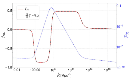
Figure 1: $f_{\mathrm{NL}}$ in the squeezed limit with $k=k_{1}=k_{2}=10^{6}k_{3}$ for the case 1. Dashed line shows $\frac{5}{12}(1-n_{s})$ and dotted line represents the power spectrum of curvature perturbations.

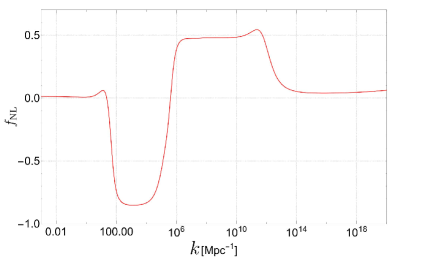
Figure 2: $f_{\mathrm{NL}}$ in the equilateral limit ($k=k_{1}=k_{2}=k_{3}$) for the case 1.

IV Effect of non-Guassianity on PBHs and SIGWS

IV.1 Non-Gaussian correction to the PBH abundance

When the large enough curvature perturbations reenter the Hubble horizon during the radiation-dominated era, the gravity of overdense regions can overcome the radiation pressure and thus these regions will collapse to form PBHs soon after their horizon entry. The PBH mass relates with the horizon mass at the horizon entry of perturbations with the wave number $k$:

$$M(k)=\gamma\frac{4\pi M_{\mathrm{pl}}^{2}}{H}\simeq M_{\odot}\left(\frac{\gamma}{0.2}\right)\left(\frac{g_{*}}{10.75}\right)^{-\frac{1}{6}}\left(\frac{k}{1.9\times 10^{6}~{}\mathrm{Mpc}^{-1}}\right)^{-2}\;,$$ (21)

where $\gamma$ denotes the ratio of the PBH mass to the horizon mass and indicates the efficiency of collapse, which is set to be $\gamma\simeq(1/\sqrt{3})^{3}$ Carr1975 in our analysis, and $g_{*}$ is the effective degrees of freedom in the energy densities at the PBH formation. We adopt $g_{*}=106.75$ since the PBHs are assumed to form deep in the radiation-dominated.

Based on the Press-Schechter theory Tada2019 ; Young2014 , the production rate of PBHs with mass $M(k)$ has the form

$$\beta(M)=\int_{\delta_{c}}\frac{d\delta}{\sqrt{2\pi\sigma^{2}(M)}}e^{-\frac{\delta^{2}}{2\sigma^{2}(M)}}=\frac{1}{2}\operatorname{erfc}\left(\frac{\delta_{c}}{\sqrt{2\sigma^{2}(M)}}\right),$$ (22)

after assuming that the probability distribution function of perturbations is Gaussian, where $\mathrm{erfc}$ is the complementary error function. $\delta_{c}$ is the threshold of the density perturbations for the PBH formation, which is chosen to be $\delta_{c}\simeq 0.4$ Musco2013 ; Harada2013 in our calculation of PBHs abundance. $\sigma^{2}(M)$ has the form

$$\sigma^{2}(M(k))=\frac{16}{81}\int d\ln q\;W^{2}\left(qk^{-1}\right)\left(qk^{-1}\right)^{4}\mathcal{P}_{\mathcal{R}}(q)\;,$$ (23)

which represents the coarse-grained density contrast with the smoothing scale $k$. Here $W$ is the window function. The current fractional energy density of PBHs with mass $M$ in dark matter is

$$f(M)\equiv\frac{1}{\Omega_{\mathrm{DM}}}\frac{d\Omega_{\mathrm{PBH}}}{d\ln M}\simeq\frac{\beta(M)}{1.84\times 10^{-8}}\left(\frac{\gamma}{0.2}\right)^{\frac{3}{2}}\left(\frac{10.75}{g_{*}}\right)^{\frac{1}{4}}\left(\frac{0.12}{\Omega_{\mathrm{DM}}h^{2}}\right)\left(\frac{M}{M_{\odot}}\right)^{-\frac{1}{2}},$$ (24)

where $\Omega_{\mathrm{DM}}$ is the current density parameter of dark matter, which is given to be $\Omega_{\mathrm{DM}}h^{2}\simeq 0.12$ by the Planck 2018 observations Aghanim2020 . For the Gaussian distribution of the curvature perturbations, we obtain PBHs with masses around $\mathcal{O}\left({10}\right)M_{\odot}$, $\mathcal{O}\left({10^{-6}}\right)M_{\odot}$, and $\mathcal{O}\left({10^{-13}}\right)M_{\odot}$, respectively and their corresponding abundances, which are shown in Tab. 2.

When the effect of non-Guassianity of the curvature perturbations on the PBH abundance is considered, the mass fraction $\beta$ is corrected to be G.Franciolini2018 ; Riccardi2021

$$\beta=\mathrm{e}^{\Delta_{3}}\beta^{G}\;,$$ (25)

where $\Delta_{3}$ is the 3rd cumulant, which has the form

$$\Delta_{3}=\frac{1}{3!}\left(\frac{\delta_{c}}{\sigma}\right)^{2}S_{3}\delta_{c},$$ (26)

with $S_{3}$ being

$$S_{3}=\frac{\left\langle\delta_{R}(\bm{x})\delta_{R}(\bm{x})\delta_{R}(\bm{x})\right\rangle}{\sigma^{4}}\;.$$ (27)

For the Gaussian window function, $\left\langle\delta_{R}(\bm{x})\delta_{R}(\bm{x})\delta_{R}(\bm{x})\right\rangle$ can be obtained through calculating

$$\left\langle\delta_{R}(\bm{x})\delta_{R}(\bm{x})\delta_{R}(\bm{x})\right\rangle = -64\left(\frac{4}{9}\right)^{3}\frac{2}{(2\pi)^{4}}k^{6}$$

$$\times \int_{0}^{\infty}du\int_{0}^{\infty}dv\int_{|u-v|}^{u+v}dwu^{3}v^{3}w^{3}\mathrm{e}^{-u^{2}}\mathrm{e}^{-v^{2}}\mathrm{e}^{-w^{2}}B_{\mathcal{R}}(\sqrt{2}uk,\sqrt{2}vk,\sqrt{2}wk).$$

In Zhang2021 , it has been found that $\Delta_{3}$ can be approximated as

$$\Delta_{3}\approx\Delta_{3}^{a}(k_{\text{peak}})=23\frac{\delta_{c}^{3}}{\mathcal{P}_{\mathcal{R}}\left(k_{\mathrm{peak}}\right)}~{}f_{\text{NL }}(k_{\mathrm{peak}},k_{\mathrm{peak}},k_{\mathrm{peak}}).$$ (29)

We numerically compute $\Delta_{3}$ and its approximation $\Delta_{3}^{a}$. The results are shown in Tab. 2 for three different cases. It is easy to see that $\Delta_{3}$ is of the order $\mathcal{O}(1)$, which is much larger than $\Delta_{3}^{a}$. Thus, the approximation given in Zhang2021 is invalid for the model considered in the present paper. We find that for all the cases the non-Gaussianity promotes the formation of PBHs since their 3rd cumulants $\Delta_{3}$ are positive. The effect of non-Gaussianity on the PBH abundance is non-negligible since the value of $\beta$ is much larger than $\beta^{G}$.

Table 2: The numerical results for three cases given in Tab. 1.

	$k_{\mathrm{peak}}/\mathrm{Mpc}^{-1}$	$\mathcal{P}_{\mathcal{R}}/10^{-2}$	$f_{\mathrm{PBH}}^{G}$	$M_{\mathrm{PBH}}/M_{\odot}$	$f_{\mathrm{NL}}$	$\Delta_{3}^{a}$	$\Delta_{3}$
Case 1	$4.46\times 10^{5}$	$4.91$	$0.00455$	$16.57$	$~{}~{}0.0205$	$~{}~{}0.619$	$~{}4.218$
Case 2	$4.31\times 10^{8}$	$3.87$	$0.0178$	$~{}~{}1.91\times 10^{-5}$	$~{}~{}0.0234$	$~{}~{}0.890$	$~{}4.965$
Case 3	$1.77\times 10^{12}$	$3.18$	$0.924$	$1.12\times 10^{-12}$	$-0.0052$	$-0.240$	$~{}6.297$

IV.2 Non-Gaussian correction to energy density of SIGWs

Associated with the PHB formation, the enhanced curvature perturbations will lead to the large scalar metric perturbations, which become the significant GW source and emit abundant SIGWs. The current energy spectra of SIGWs can be expressed as Kohri2018 ; Inomata2019

$$\Omega_{\mathrm{GW},0}h^{2}=0.83\left(\frac{g_{*}}{10.75}\right)^{-1/3}\Omega_{\mathrm{r},0}h^{2}\Omega_{\mathrm{GW}}\left(\tau_{c},k\right),$$ (30)

where $\Omega_{\mathrm{r},0}h^{2}\simeq 4.2\times 10^{5}$ is the current density parameter of radiation, and

$$\Omega_{\mathrm{GW}}\left(\tau_{c},k\right)= \frac{1}{12}\int_{0}^{\infty}dv\int_{|1-v|}^{|1+v|}du\left(\frac{4v^{2}-\left(1+v^{2}-u^{2}\right)^{2}}{4uv}\right)^{2}\mathcal{P}_{\mathcal{R}}(ku)\mathcal{P}_{\mathcal{R}}(kv)$$

$$\times\left(\frac{3}{4u^{3}v^{3}}\right)^{2}\left(u^{2}+v^{2}-3\right)^{2}$$

$$\times\bigg{\{}\left[-4uv+\left(u^{2}+v^{2}-3\right)\ln\left|\frac{3-(u+v)^{2}}{3-(u-v)^{2}}\right|\right]^{2}$$

$$+\pi^{2}\left(u^{2}+v^{2}-3\right)^{2}\Theta(v+u-\sqrt{3})\bigg{\}}\,,$$ (31)

where $\tau_{c}$ represents the time when $\Omega_{\mathrm{GW}}$ stops to grow and $\Theta$ is the Heaviside theta function.

When the non-Gaussianity of the curvature perturbations is considered, $\mathcal{R}(\bm{x})$ has the expression Verde2000 ; Komatsu2001

$$\mathcal{R}(\bm{x})=\mathcal{R}^{G}(\bm{x})+\frac{3}{5}f_{\mathrm{NL}}\left(\mathcal{R}^{G}(\bm{x})^{2}-\left\langle\mathcal{R}^{G}(\bm{x})^{2}\right\rangle\right)\,.$$ (32)

Clearly the curvature perturbation $\mathcal{R}$ consists of a Gaussian part $\mathcal{R}^{G}$ and a non-Gaussian one. When this non-Gaussian correction is included, the power spectrum of the curvature perturbations should be modified to be

$$\mathcal{P}_{\mathcal{R}}(k)=\mathcal{P}_{\mathcal{R}}^{G}(k)+\mathcal{P}_{\mathcal{R}}^{NG}(k),$$ (33)

where

$$\mathcal{P}_{\mathcal{R}}^{NG}(k)=\left(\frac{3}{5}\right)^{2}\frac{k^{3}}{2\pi}f_{\mathrm{NL}}^{2}\int d^{3}\bm{p}\frac{\mathcal{P}_{\mathcal{R}}^{G}(p)}{p^{3}}\frac{\mathcal{P}_{\mathcal{R}}^{G}(|\bm{k}-\bm{p}|)}{|\bm{k}-\bm{p}|^{3}}.$$ (34)

For the model considered in this paper, the result in the preceding subsection has shown that the absolute value of $f_{\mathrm{NL}}$ is less than one and it is near zero when $k=k_{\mathrm{peak}}$. Furthermore the maximum value of $\mathcal{P}_{\mathcal{R}}^{G}$ has the order of $\mathcal{O}(0.01)$. Thus, we can assess easily that $\mathcal{P}_{\mathcal{R}}^{NG}(k)$ is much less than $\mathcal{P}_{\mathcal{R}}^{G}(k)$ since the order of its maximum should be less than $\mathcal{O}(10^{-4})$, which indicates that the contribution of non-Gaussianity of the curvature perturbations on the energy density of SIGWs is negligible.

V conclusions

To generate a sizable amount of PBHs requires that the amplitude of the power spectrum of the curvature perturbations is enhanced to reach the $\mathcal{O}(0.01)$ order. A simple way to enhance the curvature perturbations during inflation is to reduce the rolling speed of inflaton to achieve an ultra-slow-roll inflation, which can be realized by flattening the inflationary potential or increasing the gravitational friction. Since the ultra-slow-roll inflation deviates apparently from the standard slow-roll inflation, the non-Gaussianity of the curvature perturbations might be very large and has significant effects on the abundance of PBHs and the energy density of SIGWs although it is negligible in the standard slow-roll inflation.

In this paper we study the non-Gaussianity of the curvature perturbations in the ultra-slow-roll inflation resulting from gravitationally enhanced friction. We find that at the large scales where the power spectrum of the curvature perturbations is nearly scale invariant, the non-Gaussianity is negligible. The power spectrum grows with the decrease of scale due to that the friction slows down the inflaton, and correspondingly the value of the non-Gaussianity parameter $f_{\mathrm{NL}}$ drops sharply and then stabilizes at a value in several e-folding number. Before the power spectrum reaches its peak, $f_{\mathrm{NL}}$ begins to increase rapidly. When the power spectrum is at its maximum value, we find that $f_{\mathrm{NL}}$ is nearly zero. Then, $f_{\mathrm{NL}}$ will reach its maximum value with the increase of wave number $k$. Finally, with the ending of the ultra-slow-roll inflation, $f_{\mathrm{NL}}$ returns to about zero. For three different cases, which correspond to that the PBHs can be used to explain the LIGO/Virgo GW events and the six ultrashort-timescale microlensing events in the OGLE data, and make up all dark matter, respectively, we obtain that the non-Gaussianity will promote the generation of PBHs, while its influence on SIWGs is negligible.

Appendix A The expressions of $\mathcal{B}_{\mathcal{R}}^{i}\left(k_{1},k_{2},k_{3}\right)$ in Eq. (18)

In order to compute bispectrum, we need derive the cubic action of the curvature perturbations from the action given in Eq. (1) A.D.Felice2011 ; Felice2011

$$S_{3} = \int dtd^{3}x\left\{a^{3}\mathcal{C}_{1}\mathcal{R}\dot{\mathcal{R}}^{2}+a\mathcal{C}_{2}\mathcal{R}(\partial\mathcal{R})^{2}+a^{3}\mathcal{C}_{3}\dot{\mathcal{R}}^{3}+a^{3}\mathcal{C}_{4}\dot{\mathcal{R}}\left(\partial_{i}\mathcal{R}\right)\left(\partial_{i}\chi\right)\right.$$ (35)

$$+a^{3}\mathcal{C}_{5}\partial^{2}\mathcal{R}(\partial\chi)^{2}+a\mathcal{C}_{6}\dot{\mathcal{R}}^{2}\partial^{2}\mathcal{R}+\left(\mathcal{C}_{7}/a\right)\left[\partial^{2}\mathcal{R}(\partial\mathcal{R})^{2}-\mathcal{R}\partial_{i}\partial_{j}\left(\partial_{i}\mathcal{R}\right)\left(\partial_{j}\mathcal{R}\right)\right]$$

$$+a\mathcal{C}_{8}\left[\partial^{2}\mathcal{R}\partial_{i}\mathcal{R}\partial_{i}\chi-\mathcal{R}\partial_{i}\partial_{j}\left(\partial_{i}\mathcal{R}\right)\left(\partial_{j}\chi\right)\right]+\left.\mathcal{F}_{1}\frac{\delta\mathcal{L}_{2}}{\delta\mathcal{R}}\right\},$$

where

$$\mathcal{F}_{1} = \frac{A_{4}}{w_{1}^{2}}\left\{\left(\partial_{k}\mathcal{R}\right)\left(\partial_{k}\chi\right)-\partial^{-2}\partial_{i}\partial_{j}\left[\left(\partial_{i}\mathcal{R}\right)\left(\partial_{j}\chi\right)\right]\right\}$$

$$+q_{1}\mathcal{R}\dot{\mathcal{R}}-\frac{A_{4}}{a^{2}w_{2}}\times\left\{(\partial\mathcal{R})^{2}-\partial^{-2}\partial_{i}\partial_{j}\left[\left(\partial_{i}\mathcal{R}\right)\left(\partial_{j}\mathcal{R}\right)\right]\right\},$$

$\partial^{2}\chi=Q\dot{\mathcal{R}}$, $\mathcal{L}_{2}$ is quadratic Lagrangian given in Eq. (7), $w_{i}$ and $Q$ are given in Eqs. (II) and (8), respectively, and the dimensionless coefficients $\mathcal{C}_{i}$ with $i=1-8$ are

$$\mathcal{C}_{1} = \frac{1}{M_{\mathrm{pl}}^{2}}\left[3Q+q_{1}(\dot{Q}+3HQ)-Q\dot{q}_{1}\right],$$ (36)

$$\mathcal{C}_{2} = \frac{1}{M_{\mathrm{pl}}^{2}}\left[A_{5}+\frac{1}{a}\frac{d}{dt}\left(\frac{2aQw_{1}}{w_{2}}\right)\right],$$ (37)

$$\mathcal{C}_{3} = \frac{1}{M_{\mathrm{pl}}}\left[A_{1}+A_{3}\frac{Q}{w_{1}}-q_{1}Q\right],$$ (38)

$$\mathcal{C}_{4} = \frac{Q}{w_{1}}\left[-\frac{1}{2}-w_{1}\frac{d}{dt}\left(\frac{A_{4}}{w_{1}^{2}}\right)+\frac{3HA_{4}}{w_{1}}\right],$$ (39)

$$\mathcal{C}_{5} = \frac{M_{\mathrm{pl}}^{2}}{2}\left[\frac{3}{2w_{1}}-\frac{d}{dt}\left(\frac{A_{4}}{w_{1}^{2}}\right)+\frac{3HA_{4}}{w_{1}^{2}}\right],$$ (40)

$$\mathcal{C}_{6} = A_{2}-\frac{2w_{1}A_{3}}{w_{2}},$$ (41)

$$\mathcal{C}_{7} = q_{3}+\frac{2A_{4}Qc_{s}^{2}}{w_{2}},$$ (42)

$$\mathcal{C}_{8} = M_{\mathrm{pl}}\left[\frac{q_{2}}{2}-\frac{2c_{s}^{2}A_{4}Q}{w_{1}^{2}}\right].$$ (43)

Here

$$A_{1} = \frac{3w_{1}}{w^{3}_{2}}\bigg{[}8H^{2}\left(M_{\mathrm{pl}}^{2}-5\dot{\phi}^{2}\theta\left(\phi\right)\right)w_{1}^{2}+8H\left(3\dot{\phi}^{2}\theta\left(\phi\right)-M_{\mathrm{pl}}^{2}\right)w_{1}w_{2}+\left(2M_{\mathrm{pl}}^{2}-3\dot{\phi}^{2}\theta\left(\phi\right)\right)w_{2}^{2}\bigg{]},$$

$$A_{2} = -4\dot{\phi}^{2}\theta(\phi)\frac{w_{1}^{2}}{w^{2}_{2}},$$

$$A_{3} = \frac{2w_{1}}{w^{2}_{2}}\left[4Hw_{1}\left(M_{\mathrm{pl}}^{2}-3\dot{\phi}^{2}\theta\left(\phi\right)\right)+w_{2}\left(3\dot{\phi}^{2}\theta\left(\phi\right)-2M_{\mathrm{pl}}^{2}\right)\right],$$

$$A_{4} = \frac{w_{1}}{2w_{2}}\left(3\dot{\phi}^{2}\theta\left(\phi\right)-2M_{\mathrm{pl}}^{2}\right),$$

$$A_{5} = \frac{2\dot{w}_{2}w_{1}^{2}+w_{2}\left(w_{2}w_{4}-4\dot{w}_{1}w_{1}-2Hw_{1}^{2}\right)}{w_{2}^{2}},$$

and

$$q_{1} = -\frac{2w_{1}}{c_{s}^{2}w_{2}},$$

$$q_{2} = a^{2}\frac{d}{dt}\left[\frac{w_{1}\left(4M_{\mathrm{pl}}^{2}-6\dot{\phi}^{2}\theta\left(\phi\right)\right)}{a^{2}w_{2}^{2}}\right]-\frac{4w_{1}}{w_{2}},$$

$$q_{3} = \frac{2w_{1}^{3}}{3w_{2}^{2}}-\frac{a}{3}\frac{d}{dt}\left[\frac{2w_{1}^{3}\left(3\dot{\phi}^{2}\theta(\phi)-2M_{\mathrm{pl}}^{2}\right)}{aw_{2}^{3}}\right].$$

Using the in-in formula, one can obtain the three-point correlation function from the cubic action of the curvature perturbations. The analytical expression is shown in Eq. (18), in which $\mathcal{B}_{\mathcal{R}}^{i}\left(k_{1},k_{2},k_{3}\right)$ have the forms

$$\mathcal{B}_{\mathcal{R}}^{1}\left(k_{1},k_{2},k_{3}\right)=-4\int_{t_{i}}^{t_{e}}dt\;a^{3}\;\mathcal{C}_{1}\left(\mathcal{R}_{k_{1}}^{*}(t)\dot{\mathcal{R}}_{k_{2}}^{*}(t)\dot{\mathcal{R}}^{*}_{k_{3}}(t)+\text{ perm }\right),$$ (44)

$$\mathcal{B}_{\mathcal{R}}^{2}\left(k_{1},k_{2},k_{3}\right)=4\int_{t_{i}}^{t_{e}}dt\;a\;\mathcal{C}_{2}\left[\left(\bm{k}_{1}\cdot\bm{k}_{2}+\bm{k}_{1}\cdot\bm{k}_{3}+\bm{k}_{2}\cdot\bm{k}_{3}\right)\mathcal{R}_{k_{1}}^{*}(t)\mathcal{R}_{k_{2}}^{*}(t)\mathcal{R}_{k_{3}}^{*}(t)\right],$$ (45)

$$\mathcal{B}_{\mathcal{R}}^{3}\left(k_{1},k_{2},k_{3}\right)=-12\int_{t_{i}}^{t_{e}}dt\;a^{3}\;\mathcal{C}_{3}\dot{\mathcal{R}}_{k_{1}}^{*}(t)\dot{\mathcal{R}}_{k_{2}}^{*}(t)\dot{\mathcal{R}}_{k_{3}}^{*}(t),$$ (46)

$$\mathcal{B}_{\mathcal{R}}^{4}\left(k_{1},k_{2},k_{3}\right)=-2\int_{t_{i}}^{t_{e}}dt\;a^{3}\;\mathcal{C}_{4}\;Q\left[\left(\frac{\bm{k}_{1}\cdot\bm{k}_{2}}{k_{2}^{2}}+\frac{\bm{k}_{1}\cdot\bm{k}_{3}}{k_{3}^{2}}\right)\mathcal{R}_{k_{1}}^{*}(t)\dot{\mathcal{R}}_{k_{2}}^{*}(t)\dot{\mathcal{R}}_{k_{3}}^{*}(t)+\text{ perm }\right],$$ (47)

$$\mathcal{B}_{\mathcal{R}}^{5}\left(k_{1},k_{2},k_{3}\right)=-4\int_{t_{i}}^{t_{e}}dt\;a^{3}\;\mathcal{C}_{5}\;Q^{2}\left[\frac{k_{1}^{2}\bm{k}_{2}\cdot\bm{k}_{3}}{k_{2}^{2}k_{3}^{2}}\mathcal{R}_{k_{1}}^{*}(t)\dot{\mathcal{R}}_{k_{2}}^{*}(t)\dot{\mathcal{R}}_{k_{3}}^{*}(t)+\text{ perm }\right],$$ (48)

$$\mathcal{B}_{\mathcal{R}}^{6}\left(k_{1},k_{2},k_{3}\right)=4\int_{t_{i}}^{t_{e}}dt\;a\;\mathcal{C}_{6}\left[k_{1}^{2}\mathcal{R}_{k_{1}}^{*}(t)\dot{\mathcal{R}}^{*}k_{2}(t)\dot{\mathcal{R}}^{*}k_{3}(t)+\text{ perm }\right],$$ (49)

$$\mathcal{B}_{\mathcal{R}}^{7}\left(k_{1},k_{2},k_{3}\right)=-4\int_{t_{i}}^{t_{e}}dt\;\mathcal{C}_{7}/a\left[\left(k_{1}^{2}\bm{k}_{2}\cdot\bm{k}_{3}+k_{2}^{2}\bm{k}_{1}\cdot\bm{k}_{3}+k_{3}^{2}\bm{k}_{1}\cdot\bm{k}_{2}\right)\mathcal{R}_{k_{1}}^{*}(t)\mathcal{R}_{k_{2}}^{*}(t)\mathcal{R}_{k_{3}}^{*}(t)\right],$$ (50)

$$\mathcal{B}_{\mathcal{R}}^{8}\left(k_{1},k_{2},k_{3}\right)=2\int_{t_{i}}^{t_{e}}dt\;\mathcal{C}_{7}/a {\left[\left(k_{2}^{2}\bm{k}_{2}\cdot\bm{k}_{3}+k_{3}^{2}\bm{k}_{3}\cdot\bm{k}_{2}+k_{1}^{2}\bm{k}_{1}\cdot\bm{k}_{2}+k_{1}^{2}\bm{k}_{1}\cdot\bm{k}_{3}\right.\right.}$$

$$\left.\left.+k_{2}^{2}\bm{k}_{2}\cdot\bm{k}_{1}+k_{3}^{2}\bm{k}_{3}\cdot\bm{k}_{1}\right)\mathcal{R}_{k_{1}}^{*}(t)\mathcal{R}_{k_{2}}^{*}(t)\mathcal{R}_{k_{3}}^{*}(t)\right],$$ (51)

$$\mathcal{B}_{\mathcal{R}}^{9}\left(k_{1},k_{2},k_{3}\right)=2\int_{t_{i}}^{t_{e}}dt\;a\;\mathcal{C}_{8}\;Q\left[\left(\frac{k_{1}^{2}\bm{k}_{2}\cdot\bm{k}_{3}}{k_{3}^{2}}+\frac{k_{2}^{2}\bm{k}_{1}\cdot\bm{k}_{3}}{k_{3}^{2}}\right)\mathcal{R}_{k_{1}}^{*}(t)\mathcal{R}_{k_{2}}^{*}(t)\dot{\mathcal{R}}_{k_{3}}^{*}(t)+\text{ perm }\right],$$ (52)

$$\mathcal{B}_{\mathcal{R}}^{10}\left(k_{1},k_{2},k_{3}\right)=-2\int_{t_{i}}^{t_{e}}dt\;a\;\mathcal{C}_{8}\;Q\left[\left(\frac{k_{2}^{2}\bm{k}_{2}\cdot\bm{k}_{3}}{k_{3}^{2}}+\frac{k_{1}^{2}\bm{k}_{1}\cdot\bm{k}_{3}}{k_{3}^{2}}\right)\mathcal{R}_{k_{1}}^{*}(t)\mathcal{R}_{k_{2}}^{*}(t)\dot{\mathcal{R}}_{k_{3}}^{*}(t)+\operatorname{perm}\right].$$ (53)